



1. Introduction
Hydraulic jumps are waves that connect sections of strongly varying flows. They have been observed by famous authors, including Leonardo da Vinci, Bidone (Reference Bidone1819), Savart (Reference Savart1833), Bélanger (Reference Bélanger1841) and Rayleigh (Reference Rayleigh1914). The last two introduced the well-known conservation laws at the jump for mass and momentum, Rayleigh being able to derive these from a continuous description of the thickness profile. At the position of the jump, the flow speed,
 $v$
, decreases drastically from supersonic to subsonic with respect to the local surface wave speed. In a thin layer of height
 $h$
, the speed of gravity waves is given by
 $\sqrt{gh}$
, where
 $g$
is the acceleration due to gravity. The corresponding dimensionless number is the Froude number,
 $\mathit{Fr}=v/\sqrt{gh}$
, where the velocity
 $v$
is defined with respect to the reference frame where the hydraulic jump is standing. The flow upstream of the jump, being more rapid than the surface waves, is referred to as supercritical with
 $\mathit{Fr}>1$
, while the flow downstream of the jump is referred to as subcritical with
 $\mathit{Fr}<1$
. This allows the vision of the hydraulic jump as a shock wave, in analogy with compressible gas flows (Lighthill Reference Lighthill1978), and in which a hypothetical transition would be localized at a place where
 $\mathit{Fr}=1$
. The Mach cone, which is a characteristic of supercritical flows, has been observed in radial hydraulic jumps by Jannes et al. (Reference Jannes, Piquet, Maissa, Mathis and Rousseaux2011), who suggested a possible transition governed by
 $\mathit{Fr}=1$
at the jump position. In rivers, hydraulic jumps, whose position is almost stationary, appear because of variations of the river bed (Chow Reference Chow1959; Simpson Reference Simpson1997). Tidal bores, which are wavefronts associated with a tide propagating in the opposite direction to the river current, can also be interpreted as moving hydraulic jumps (Chanson Reference Chanson2011). These natural objects, which share the same characteristic high Reynolds number,
 $\mathit{Re}$
, do exhibit turbulent flows that provide strong variations of the surface profile.
In order to probe flows with moderately high Reynolds number, hydraulic jumps might be created by impacting a jet on a solid surface, as in the common operation of opening the tap of a kitchen sink. The obtained hydraulic jump takes a circular form whose radius depends on the viscosity (Watson Reference Watson1964; Craik et al.
Reference Craik, Latham, Fawkes and Gribbon1981; Bohr, Putkaradze & Watanabe Reference Bohr, Putkaradze and Watanabe1993), and is not directly given by the
 $\mathit{Fr}=1$
criterion (applied to a hypothetical inertial flow that in fact never holds). At the centimetre scale and in this geometry, the formation mechanism appears to be a coupling between the boundary layer emerging from the solid substrate and the free surface (Watson Reference Watson1964; Bowles & Smith Reference Bowles and Smith1992; Higuera Reference Higuera1994). Craik et al. (Reference Craik, Latham, Fawkes and Gribbon1981) partially observed the existence of a reverse flow, which takes the form of a toroidal vortex and acts like a springboard for the incoming fluid. This separation of the boundary layer might be explained by the existence of an adverse pressure gradient, as proposed by Kurihara (Reference Kurihara1946) and Tani (Reference Tani1949). Theoretical approaches (Watson Reference Watson1964; Bohr, Putkaradze & Watanabe Reference Bohr, Putkaradze and Watanabe1997; Rojas et al.
Reference Rojas, Argentina, Cerda and Tirapegui2010) and numerical techniques (Yokoi & Xiao Reference Yokoi and Xiao2002; Passandideh-Fard, Teymourtash & Khavari Reference Passandideh-Fard, Teymourtash and Khavari2011) have also evidenced this peculiar flow. Various scaling laws predict a viscosity dependence for the radius position (Watson Reference Watson1964; Bohr et al.
Reference Bohr, Putkaradze and Watanabe1997; Bush & Aristoff Reference Bush and Aristoff2003; Rojas, Argentina & Tirapegui Reference Rojas, Argentina and Tirapegui2013; Duchesne, Lebon & Limat Reference Duchesne, Lebon and Limat2014). In addition, the experimental measurements of Duchesne et al. (Reference Duchesne, Lebon and Limat2014) show the occurrence at the exit of circular hydraulic jumps of a locked value of the Froude number, whose value is independent of the flow rate imposed by the jet. One-dimensional hydraulic jumps, which have been addressed by Bonn, Andersen & Bohr (Reference Bonn, Andersen and Bohr2008), are slightly different, since the upstream fluid thickness increases almost linearly in space. The hydraulic jumps created by the impact jet present the advantage of being almost laminar, but the formation mechanism appears to be also deeply linked to viscous effects.
We describe here a new kind of hydraulic jump, where the driving force has a capillary origin, gravitational effects can be omitted, and viscosity does not play a fundamental role in the formation mechanism. In a thin layer of thickness
 $l$
, the characteristic surface wave velocity behaves as
 $\sqrt{{\it\gamma}/{\it\rho}l}$
, where
 ${\it\rho}$
is the density of the fluid and
 ${\it\gamma}$
its surface tension. In such a case, the Froude number introduced in the Rayleigh theory is replaced by the Weber number
 $\mathit{We}={\it\rho}v^{2}l/{\it\gamma}$
. Consequently, there exists a critical Weber number
 $\mathit{We}_{c}$
below which surface waves cannot travel faster than the fluid flow. A capillary-driven hydraulic jump is expected in flows for which
 $\mathit{We}-\mathit{We}_{c}$
changes its sign. This scenario should be potentially observed in thin films falling down an inclined plane, as depicted by Kapitza (Reference Kapitza1948), in which capillary effects might dominate gravity. Nevertheless, the small length scale also introduces notable viscous shear, which affects the shock-wave criterion.
Optical photography of a liquid foam. The close-up shows a Plateau border. The grey areas represent the liquid films shared by two adjacent bubbles.

In this article, we present capillary hydraulic jumps, analogous to hydraulic jumps, formed in a Plateau border (PB). Plateau’s laws describe the geometric properties of interacting soap films. At equilibrium, they always meet in threes, creating a microchannel, called a Plateau border (see figure 1). PBs merge into nodes and the PB–node network creates a porous medium that mediates the liquid flows. Usually, drainage in a gravitational field can be described using low-Reynolds-number flows in a Darcy-like approach (Weaire et al.
Reference Weaire, Pittet, Hutzler and Pardal1993; Koehler, Hilgenfeldt & Stone Reference Koehler, Hilgenfeldt and Stone1999). In capillary suction experiments, flow is triggered by capillary effects due to PB thickness inhomogeneities. In that case, the Ohnesorge number
 $\mathit{Oh}=\sqrt{\mathit{We}}/\mathit{Re}$
discriminates between different regimes for fluid flow (Cohen et al.
Reference Cohen, Fraysse, Rajchenbach, Argentina, Bouret and Raufaste2014). We have used here
 $\mathit{Re}={\it\rho}vl/{\it\eta}$
, where the fluid viscosity is
 ${\it\eta}$
. For
 $\mathit{Oh}>0.05$
, PB perturbations disappear through viscous damping, whereas for
 $\mathit{Oh}<0.05$
, inertia dominates the flow and a wave, similar to a hydraulic jump, propagates along the PB with an almost constant velocity. This is the regime we address in this study.
This article is organized as follows. Section 2 describes a simple model for capillary jumps in PBs. The comparison between our theoretical predictions and our experimental measurements are presented in § 3. In § 4, we propose an energetic argument providing a selection mechanism for capillary jumps.
2. Model
The model aims at computing the shape and velocity of the capillary jump. We consider the Plateau border depicted in figure 2: the three holding films are attached to a triangular prism frame; the liquid flows along the
 $z$
axis; and
 $R_{ext}$
defines the radius of the circum-circle of the equilateral triangles defining the holding frame.
(a) Three-dimensional representation of the system. The grey surfaces represent the liquid–air interfaces. The dashed lines represent equilateral triangles with a circum-circle of radius
 $R_{ext}$
. (b) Arbitrary cross-section of the system showing the Plateau border with its three holding films. The thick curves represent liquid–air interfaces. The thickness,
 $e$
, of the PB is proportional to its radius of curvature,
 $R$
.

The interior region delimited by the arcs
 $\widehat{AB}$
,
 $\widehat{BC}$
and
 $\widehat{CA}$
defines the PB channel. We assume a constant pressure
 $P_{ext}$
in the surrounding air. Laplace’s law predicts the radius of curvature of the arcs as
 $R={\it\gamma}/(P_{ext}-P)$
, such that the cross-section of the PB is symmetric, since all the surfaces of the channel share the same curvature. Here
 ${\it\gamma}$
is the surface tension and
 $P$
the pressure inside the fluid. The channel thickness
 $e=(\sqrt{3}/2)R$
is defined as the height of the equilateral triangle
 $ABC$
. The segments
 $AA^{\prime }$
,
 $BB^{\prime }$
and
 $CC^{\prime }$
represent the three films composed of two interfaces separating the fluid from the air.
We denote by
 $\mathscr{P}={\rm\pi}R$
the PB perimeter and by
 $\mathscr{A}={\it\alpha}R^{2}$
its cross-sectional area, with
 ${\it\alpha}=\sqrt{3}-({\rm\pi}/2)$
. The length
 $\mathscr{L}$
of the interfaces on the cross-section is the sum of the perimeter
 $\mathscr{P}$
and six times the distance
 $AA^{\prime }$
(the factor 2 arises because each film is composed of two liquid–air interfaces):
 $$\begin{eqnarray}\mathscr{L}=-2{\it\alpha}R+6R_{ext}.\end{eqnarray}$$
As a consequence, the area of the liquid–air interfaces of the system decreases as
 $R$
increases, as pointed out by Géminard et al. (Reference Géminard, Zywocinski, Caillier and Oswald2004). The PB capillary energy, proportional to
 $\mathscr{L}$
, decreases as the PB thickness
 $e$
increases. From an energetic point of view, the PB tends to increase its size
 $e$
, which is a necessary condition for the existence of a capillary jump.
The model derivation is based on the following assumptions.
-
(i) The flow is laminar and characterized by a high Reynolds number.
-
(ii) The pressure
 $P$
and the longitudinal velocity
$u$
inside the channel depend only on
$z$
.
-
(iii) The variations of all the physical variables are small in the
$z$
direction.


The jump propagates with a constant velocity of amplitude
 $c$
towards a region where the fluid velocity is zero and
 $R=R_{i}$
. Experimentally, the injection of fluid inside the PB, initially at rest with
 $R=R_{i}$
, might create the jump as the fluid excess propagates (see § 3).
The system is described in the reference frame of the capillary jump, where the flow is steady, as shown in figure 3. With the variable
 $Z$
attached to the reference frame of the front (
 $Z=z-ct$
, with
 $z$
the variable in the laboratory frame), the mass conservation is written as
 $$\begin{eqnarray}\partial _{Z}(u\mathscr{A})=0,\end{eqnarray}$$
where we have neglected the mass flow inside the films, since their area in the cross-section is negligible compared to
 $\mathscr{A}$
. We write the longitudinal momentum conservation in a slice of fluid between
 $Z$
and
 $Z+\text{d}Z$
as
 $$\begin{eqnarray}\partial _{Z}[\mathscr{A}({\it\rho}u^{2}+P-P_{ext}-{\it\sigma}_{zz})-{\it\gamma}\mathscr{L}]=0.\end{eqnarray}$$
Longitudinal section of the capillary jump, in its reference frame. The jump moves to the right with a velocity
 $c$
in the laboratory frame.

The first term in the momentum flux arises from the flow inside the channel. Surface tension exerts a longitudinal force proportional to
 $\mathscr{L}$
pointing outwards from the infinitesimal cylinder. Longitudinal flows inside the films have been neglected with respect to those inside the channel. The term
 ${\it\sigma}_{zz}=2{\it\eta}\partial _{Z}u$
is the viscous shear stress applied to the cross-section oriented in the
 $Z$
direction. The fluid pressure
 $P$
, evaluated at the fluid surface, obeys the dynamic boundary condition
 $$\begin{eqnarray}P+{\it\gamma}{\it\kappa}=P_{ext}+{\it\sigma}_{rr}\quad \text{on }\widehat{AB},\widehat{BC},\widehat{CA},\end{eqnarray}$$
valid in the limit of small longitudinal deformations of the interfaces. Here
 ${\it\sigma}_{rr}$
is the normal fluid shear stress applied to the surface of the PB. The mean curvature
 ${\it\kappa}$
can be written as
 $$\begin{eqnarray}{\it\kappa}=\frac{1}{R(Z)}+{\it\beta}_{1}R^{\prime \prime }(Z)+{\it\beta}_{2}\frac{R^{\prime }(Z)^{2}}{R(Z)},\end{eqnarray}$$
obtained in the small slope limit (see appendix A), where
 ${\it\beta}_{1,2}$
are geometrical coefficients. To close the model, we compute an approximation of the viscous stress
 ${\it\sigma}_{rr}=2{\it\eta}\partial _{r}u_{r}$
, with
 $u_{r}$
defined as the radial velocity. The fluid is incompressible, and we relate the radial velocity with the longitudinal velocity using the divergence-free flow relation following an idea developed by Bogy (Reference Bogy1979):
 $$\begin{eqnarray}\frac{1}{r}\partial _{r}(ru_{r})+\partial _{Z}u=0,\end{eqnarray}$$
where the angular dependence has been disregarded. Integrating this relation gives
 $u_{r}=-(r/2)\partial _{Z}u$
. Consequently, the radial viscous stress approximates to
 $$\begin{eqnarray}{\it\sigma}_{rr}=-{\it\eta}\partial _{Z}u.\end{eqnarray}$$
This rough approximation gives
 ${\it\sigma}_{rr}$
that is similar to the radial shear stress in cylindrical jets. Inserting (2.1), (2.4), (2.5) and (2.7) into (2.3) yields
 $$\begin{eqnarray}\partial _{Z}\left[\mathscr{A}\left({\it\rho}u^{2}+{\it\gamma}\left(\frac{1}{R}-{\it\beta}_{1}\partial _{ZZ}R-{\it\beta}_{2}\frac{(\partial _{Z}R)^{2}}{R}\right)-3{\it\eta}\partial _{Z}u\right)\right]=0.\end{eqnarray}$$
Note that the sign of the
 $1/R$
coefficient has changed with respect to the mean curvature expression (2.5), owing to the tension induced by the holding films. These latter generate a homogeneous pressure as is the case for cylindrical jets. The equation (2.8) is integrated to give
 $$\begin{eqnarray}{\it\rho}u^{2}+{\it\gamma}\left(\frac{1}{R}-{\it\beta}_{1}\partial _{ZZ}R-{\it\beta}_{2}\frac{(\partial _{Z}R)^{2}}{R}\right)-3{\it\eta}\partial _{Z}u=\frac{d}{R^{2}},\end{eqnarray}$$
where the integration constant
 $d$
is determined by the boundary conditions.
Because of the Galilean invariance, we assume that, in the laboratory frame, the capillary jump propagates with a velocity
 $c$
towards
 $z\rightarrow +\infty$
, at which
 $R=R_{i}$
, as shown in figure 3. The value of
 $R$
at
 $z\rightarrow -\infty$
is denoted
 $R_{j}$
. We summarize the boundary conditions as follows:
 $$\begin{eqnarray}\displaystyle u(\infty ) & = & \displaystyle -c,\end{eqnarray}$$
 $$\begin{eqnarray}\displaystyle R(-\infty ) & = & \displaystyle R_{j},\end{eqnarray}$$
 $$\begin{eqnarray}\displaystyle R(\infty ) & = & \displaystyle R_{i}.\end{eqnarray}$$
Using
 $R_{i}$
and
 $c$
as the characteristic length and velocity of the system, we rescale the physical quantities as
 $u=cv$
,
 $R=R_{i}a$
and
 $Z=R_{i}s$
. The set of equations (2.2) and (2.9) becomes
 $$\begin{eqnarray}\displaystyle & \displaystyle v=-\frac{1}{a^{2}}, & \displaystyle\end{eqnarray}$$
 $$\begin{eqnarray}\displaystyle & \displaystyle \frac{1}{a^{4}}-\frac{d_{2}}{a^{2}}+\frac{1}{\mathit{We}}\left(\frac{1}{a}-{\it\beta}_{1}\partial _{ss}a-{\it\beta}_{2}\frac{(\partial _{s}a)^{2}}{a}\right)-\frac{1}{\mathit{Re}}\frac{6}{a^{3}}\partial _{s}a=0, & \displaystyle\end{eqnarray}$$
 $d_{2}$
is the dimensionless integration constant arising from
 $d$
. We have introduced the Weber number
 $\mathit{We}$
and the Reynolds number
 $\mathit{Re}$
:
 $$\begin{eqnarray}\mathit{We}=\frac{{\it\rho}c^{2}R_{i}}{{\it\gamma}},\quad \mathit{Re}=\frac{{\it\rho}cR_{i}}{{\it\eta}}.\end{eqnarray}$$
The capillary jump velocity
 $c$
is still an unknown. Two boundary conditions fix
 $d_{2}$
and
 $\mathit{We}$
. Imposing (2.12) on (2.14) settles
 $d_{2}=1+(1/\mathit{We})$
. The boundary condition (2.11) gives the following relation:
 $$\begin{eqnarray}\mathit{We}=\tilde{r}^{2}\frac{1}{1+\tilde{r}},\end{eqnarray}$$
where we have introduced the ratio
 $\tilde{r}=R_{j}/R_{i}$
. The capillary jump velocity is deduced from (2.15a,b
) and (2.16):
 $$\begin{eqnarray}c=\sqrt{\frac{{\it\gamma}}{{\it\rho}R_{i}}}\,\tilde{r}\,\frac{1}{\sqrt{1+\tilde{r}}},\end{eqnarray}$$
such that the propagation velocity is proportional to the capillary wave velocity
 $c_{0}=\sqrt{{\it\gamma}/{\it\rho}R_{i}}$
, and a geometrical factor that depends only on the ratio
 $\tilde{r}$
. The Reynolds number defined in (2.15a,b
) becomes
 $$\begin{eqnarray}\mathit{Re}=\frac{1}{\mathit{Oh}}\frac{\tilde{r}}{\sqrt{1+\tilde{r}}},\end{eqnarray}$$
where
 $\mathit{Oh}={\it\eta}/\sqrt{{\it\rho}{\it\gamma}R_{i}}$
is the Ohnesorge number, which is the ratio of viscous stresses induced by capillary waves to inertia.
Dependence of the potential energy
 $\mathscr{U}$
on
 $\mathit{We}$
: (a)
 $\mathit{We}=0.1$
; (b)
 $\mathit{We}=1/2$
; (c)
 $\mathit{We}=1$
.

Equation (2.14) presents a nice analogy with the differential equations of mechanical nonlinear oscillators, since it may be written in the following form:
 $$\begin{eqnarray}\frac{{\it\beta}_{1}}{\mathit{We}}\partial _{ss}a+f(a,\mathit{Re},\mathit{We})\partial _{s}a+\partial _{a}\mathscr{U}=0.\end{eqnarray}$$
The dimensionless space variable
 $s$
is analogous to the temporal variable
 $t$
of oscillators. As usual, the first term represents the acceleration. A dissipation function appears in factor of
 $\partial _{s}a$
, i.e.
 $f(a,\mathit{Re},\mathit{We})=6/(a^{3}\mathit{Re})+{\it\beta}_{2}(\partial _{s}a/a\mathit{We})$
. This analogy suggests that
 $\mathscr{U}=1/(3a^{3})-(1+1/\mathit{We})/a-\ln (a)/\mathit{We}$
stands for an effective potential energy, which is plotted in figure 4. The function
 $\mathscr{U}$
has one maximum and one minimum, given the physical constraint
 $a>0$
.
2.1. Capillary jump
The capillary jump is the heteroclinic trajectory that connects two extrema of
 $\mathscr{U}$
, namely for
 $a(-\infty )=R_{j}/R_{i}$
and
 $a(\infty )=1$
. As consequence,
 $a=R_{j}/R_{i}$
must be the position of the maximum of
 $U$
, whereas
 $a=1$
must be the position of the finite minimum of
 $\mathscr{U}$
. This last condition,
 $\partial _{aa}U|_{a=1}>0$
, turns into
 $$\begin{eqnarray}\mathit{We}>{\textstyle \frac{1}{2}}.\end{eqnarray}$$
The analogy with Rayleigh theory for hydraulic jumps becomes straightforward. A capillary jump with
 $R_{j}>R_{i}$
exists only if
 $We>1/2$
, which is equivalent to the supercritical criterion
 $\mathit{Fr}>1$
for hydraulic jumps. Owing to the oscillating nature of (2.19), undulations are expected during the relaxation of
 $a$
to 1. Two numerical profiles are shown in figure 5(a). For low values of the Reynolds number, the viscous forces dominate the inertia, and
 $a$
becomes monotonic. The oscillation wavelength is assessed from a linear analysis of (2.19) around
 $a=1$
by studying the dynamics of a perturbation
 $b=a-1$
:
 $$\begin{eqnarray}\frac{{\it\beta}_{1}}{\mathit{We}}\partial _{ss}b+\frac{6}{\mathit{Re}}\partial _{s}b+\left(2-\frac{1}{\mathit{We}}\right)=0.\end{eqnarray}$$
Since this equation is linear, imposing
 $b\sim \text{e}^{qs}$
yields
 $$\begin{eqnarray}q=-3\frac{\mathit{We}}{{\it\beta}_{1}\mathit{Re}}\pm \text{i}\frac{1}{\sqrt{{\it\beta}_{1}}}\sqrt{2\mathit{We }-1}+o\left(\frac{1}{\mathit{Re}}\right)^{2}.\end{eqnarray}$$
For small Reynolds number, viscosity damps oscillations, as the real part of
 $q$
becomes very high. The dimensional wavelength
 ${\it\lambda}=2{\rm\pi}R_{i}/\text{Im}(q)$
is
 $$\begin{eqnarray}{\it\lambda}=R_{i}\frac{2{\rm\pi}\sqrt{{\it\beta}_{1}}}{\sqrt{2\mathit{We }-1}}\end{eqnarray}$$
Plateau border profiles. (a) Capillary jumps numerically computed for
 $\mathit{We}=4/3$
(equivalent to
 $\tilde{r}=2$
). Solid and dashed curves have been obtained for
 $\mathit{Re}=60$
and
 $\mathit{Re}=10$
, respectively. (b) Solitary wave profile, for very low viscosities, obtained numerically from (2.24) with
 $\mathit{We}=1/6$
.

2.2. Solitary wave
In the case where viscous shear can be neglected, i.e.
 $\mathit{Re}\gg 1$
, our model predicts the existence of solitary waves, which are homoclinic orbits connected to
 $a=1$
. In this parameter regime, (2.14) multiplied by
 $a^{2}\partial _{s}a$
and integrated with respect to the variable
 $s$
reduces to
 $$\begin{eqnarray}\frac{a(s)^{2}(1-{\it\beta}a^{\prime }(s)^{2})}{2\mathit{We}}-\frac{(\mathit{We}+1)a(s)}{\mathit{We}}-\frac{1}{a(s)}=E.\end{eqnarray}$$
To derive the previous relation, we have assumed
 ${\it\beta}_{1}={\it\beta}_{2}={\it\beta}$
, since
 ${\it\beta}_{1}$
and
 ${\it\beta}_{2}$
have almost the same numerical value (see appendix A). The boundary conditions
 $a(\infty )=1$
and
 $a^{\prime }(\infty )=0$
fix the value
 $E=-(1+4\mathit{We})/2\mathit{We}$
. Finally, the profile minimum
 $a_{m}=2\mathit{We}$
is obtained by solving (2.24) with
 $a^{\prime }(s)=0$
. A typical spatial profile of the solitary wave is shown in figure 5(b); its velocity is deduced from (2.16) as
 $$\begin{eqnarray}c=c_{0}\sqrt{\frac{a_{m}}{2}}.\end{eqnarray}$$
Physically, these waves take the form of a localized constriction of the Plateau border, travelling with a constant speed. A localized perturbation yielding a localized contraction might generate two of these solitary waves travelling in opposite directions. These structures are not connected to an external reservoir, like the previously described capillary jumps.
(a) Cross-section of the unperturbed Plateau border. Here
 $R_{i}=0.261~\text{mm}$
. (b) Longitudinal view of a propagating capillary jump on the Plateau border (solution I).

3. Experimental study
3.1. Materials and methods
In order to create the Plateau border, we constructed a
 $15~\text{mm}$
long triangular-prism frame. After dipping it into a soapy solution, the PB appears in the longitudinal direction. The frame is positioned to settle the PB horizontally, and rotated around its longitudinal axis such that the channel profile adopts the Y shape shown in figures 2 and 6(a). We can vary the radius of curvature of the PB,
 $R_{i}$
(see figure 6
a), by injecting liquid at one upper corner of the frame. In this study, we have used two liquid solutions leading to tangential-stress-free interfaces (Pitois, Fritz & Vignes-Adler Reference Pitois, Fritz and Vignes-Adler2005; Raufaste, Foulon & Dollet Reference Raufaste, Foulon and Dollet2009).
-
(i) Solution I was obtained by adding 5 % of a commercial dishwashing liquid (Dreft, Procter & Gamble) to deionized water. The physical properties of solution I are
${\it\rho}=980~\text{kg}~\text{m}^{-3}$
,
${\it\gamma}=26~\text{mN}~\text{m}^{-1}$
and
${\it\eta}=1.08~\text{mPa}~\text{s}$
. -
(ii) Solution II was obtained by dissolving tetradecyl trimethyl ammonium bromide (TTAB) in deionized water. The physical properties of solution II are
${\it\rho}=1030~\text{kg}~\text{m}^{-3}$
,
${\it\gamma}=36~\text{mN}~\text{m}^{-1}$
and
${\it\eta}=1.04~\text{mPa}~\text{s}$
.




For both solutions, the density
 ${\it\rho}$
was measured by weighing a known volume of solution (error of
 $\pm 50~\text{kg}~\text{m}^{-3}$
), the dynamic viscosity
 ${\it\eta}$
was determined using a Ubbelohde viscometer (error of
 $\pm 2\,\%$
) and the surface tension
 ${\it\gamma}$
was measured using the pendant drop method (error of
 $\pm 1~\text{mN}~\text{m}^{-1}$
), as described in Hansen & Rødsrud (Reference Hansen and Rødsrud1991).
Experiments are backlit and recorded from the side by means of a high-speed camera (1000–2000 frames per second), in order to follow the temporal evolution of the Plateau border (figure 7). A calibration step is performed before each set of experiments, which consists in coupling cross-sectional and longitudinal views, in order to deduce the radius of curvature
 $R$
of the Plateau border from its apparent thickness,
 $e$
; this calibration gives
 $R_{i}=(1.08\pm 0.02)e_{i}$
.
Snapshots of a Plateau border with two propagating capillary jumps. The pictures are recorded every 2.5 ms. (a) A droplet is released from above. (b) It coalesces with the PB. (c) Two capillary jumps are formed, one on each side of the droplet. (d–g) They propagate along the PB. (h,i) They reach the nodes. The two dashed lines are for guidance only, to show that a steady regime is reached.

(a) Space–time diagram of the thickness of the capillary jump for solution I. The darkest (lightest) grey represents 0.582 mm (0.216 mm) for the thickness of the PB. (b) Comparison with the model of the capillary jump profile observed for solution I. Grey discs represent the experimental thickness of the PB measured optically and renormalized by the thickness
 $e_{i}$
of the PB at the entrance. The experimental radii of curvature of the PB upstream and downstream of the jump are
 $R_{i}=0.30~\text{mm}$
and
 $R_{j}=0.57~\text{mm}$
, respectively. Equation (2.16) gives
 $We=1.35$
and
 $Re=95$
, when computed with a velocity
 $c=0.28~\text{m}~\text{s}^{-1}$
deduced from (2.17) and the physical values of solution I. This sets the profile
 $a(s)$
(black curve) predicted by (2.14).

3.2. Experimental results and comparison with the model
To create a capillary jump, we perturb the Plateau border by releasing a small droplet of the same surfactant solution from above, as seen in figure 7(a). After a transient time, a permanent regime sets in and two propagative capillary jumps are created on the two sides of the droplet, as pictured in figure 7. The droplet radius, which varies in our experiments from
 $0.2$
to
 $1.8~\text{mm}$
, does not play a significant role in the characteristics of the capillary jumps (see Cohen et al.
Reference Cohen, Fraysse, Rajchenbach, Argentina, Bouret and Raufaste2014). As an example, we show in supplementary movie 1 (available at http://dx.doi.org/10.1017/jfm.2014.717) a jump formation following drop coalescence at one edge of the PB. After a short transient regime, observed on a length scale given approximately by the perturbation size, these structures propagate steadily with a constant velocity,
 $c$
, and exhibit small spatial oscillations near the jumps as shown in figure 6(b). This is illustrated by supplementary movie 2. A space–time diagram of the apparent PB thickness (figure 8
a) demonstrates that
 $c$
remains constant during the propagation. This diagram was constructed as follows. The set of pictures (one example of which is shown in figure 6
b) extracted from a movie was binarized to discriminate the PB from the air. For each binarized picture, the liquid thickness profile is computed (one example is shown in figure 8
b) and is associated to a grey scale. This settles the horizontal line for this given time in the space–time diagram.
3.2.1. Capillary jump profile
The PB profile exhibits damped spatial undulations upstream (see figure 6
b). These wavy deformations are stationary in the reference frame of the capillary jump, as shown in the space–time diagram of the PB thickness in figure 8(a). To compare the experimental profile to our model, we use a Runge–Kutta method, precise at fourth order, as numerical scheme (Press et al.
Reference Press, Teukolsky, Vetterling and Flannery2007). In order to compute the spatial evolution of
 $a(s)$
, we first use the experimental values of
 $R_{i}$
and
 $R_{j}$
to obtain
 $\mathit{We}$
through (2.16). The capillary jump velocity
 $c$
is computed from (2.17), and used to evaluate
 $\mathit{Re}$
. The numerical profile is then computed via a shooting method with the initial boundary conditions
 $a(0)=R_{j}/R_{i}$
and
 $a^{\prime }(0)=-{\it\epsilon}$
. The small parameter
 ${\it\epsilon}$
controls the position of the capillary jump, but does not affect the shape of
 $a(s)$
since (2.14) is invariant under space translation. We choose
 ${\it\epsilon}$
in order to superimpose the profile onto the experimental one, as can be seen in figure 8(b). The numerical integration of (2.14) matches very well with the experimental observation, although the model has been derived within a small slope approximation. The model nicely captures the undulations together with the typical size of the jump. The dissipation model does not accurately predict the maxima of the oscillations: a much more precise description of the shear stresses including the angular dependence has to be developed. Nevertheless, our present model already captures the fundamental physics of the capillary jump.
3.2.2. Capillary jump aspect ratio
In figure 9(a), we show the measured radius
 $R_{j}$
of curvature of the PB downstream of the jump, for the two solutions I and II:
 $R_{j}$
is plotted as a function of the measured initial radius of curvature of the PB,
 $R_{i}$
. For each liquid solution, the data points coalesce onto a line. A linear regression gives
 $R_{j}=(1.93\pm 0.03)R_{i}$
for solution I and
 $R_{j}=(1.54\pm 0.03)R_{i}$
for solution II. For each solution, the ratio
 $R_{j}$
to
 $R_{i}$
appears to be constant within a good accuracy. This aspect ratio is the input parameter of our model and sets the geometrical factor of (2.17) to 1.13 and 0.96, and the Weber number of (2.16) to 1.27 and 0.92 for solutions I and II, respectively.
3.2.3. Capillary jump velocity
We measured the velocity of the jumps for solutions I and II. Figure 9(b) shows the dependence of the jump velocity on
 $R_{i}$
. For both solutions, a linear regression of the experimental points yields a scaling with a power law
 $-0.50$
for the jump velocity. Figure 9(b) shows the remarkable agreement between our model prediction and the experimental measurements.
(a) Plot of
 $R_{j}$
versus
 $R_{i}$
, measured for solution I (black markers) and solution II (grey markers). The black and grey curves represent
 $R_{j}/R_{i}=1.93$
and
 $R_{j}/R_{i}=1.54$
, respectively. (b) Velocity of the capillary jump as a function of
 $R_{i}$
(logarithmic scales), measured on solution I (black markers) and solution II (grey markers). The black and grey solid lines are the velocity predictions using (2.17) for each data set.

3.2.4. Upstream undulations
As observed by Craik et al. (Reference Craik, Latham, Fawkes and Gribbon1981) in radial hydraulic jumps, capillary waves might decorate the jump rim, in the supercritical regime. The capillary jump shares this property. These steady undulations travel with the structure. We have measured the wavelength,
 ${\it\lambda}$
, in experiments with liquid solution I, and these are reported in figure 10. The best linear fit gives
 ${\it\lambda}=(1.8\pm 0.02)R_{i}$
whereas our model predicts
 ${\it\lambda}=1.6R_{i}$
, and slightly underestimates the experimental wavelengths.
Wavelength
 ${\it\lambda}$
versus
 $R_{i}$
, measured on capillary jumps observed for solution I. The dashed line represents the best linear fit
 ${\it\lambda}=(1.78\pm 0.1)R_{i}$
. The continuous line
 ${\it\lambda}=1.6R_{i}$
stands for the model prediction of equation (2.23).

4. Selection mechanism of the capillary jump
In all the preceding sections, the capillary jump aspect ratio
 $R_{j}/R_{i}$
was required as an input parameter for the model to retrieve the experimental observations: jump profile, front velocity and undulation wavelengths. Experimentally, this aspect ratio is found to be independent of the size of the released droplet (data not shown), and thus constant for a given liquid solution. In what follows, we assume that the jump is self-adapting in shape independently of the perturbation that created it and we show that a simple energetic argument predicts the value
 $R_{j}/R_{i}$
chosen by the system. The excess of energy injected at
 $\pm \infty$
is viscously dissipated within the whole channel. Following Landau & Lifshitz (Reference Landau and Lifshitz1987), the energy balance is written as
 $$\begin{eqnarray}\displaystyle \left[\mathscr{A}u\left(\frac{{\it\rho}u^{2}}{2}+(P-P_{ext})\right)+{\it\gamma}\mathscr{L}u\right]_{-\infty }^{\infty }=-\int _{-\infty }^{\infty }\int _{\mathscr{A}}{\rm\Phi}\,\text{d}\mathscr{A}\,\text{d}z, & & \displaystyle\end{eqnarray}$$
where
 ${\rm\Phi}$
is the viscous dissipation per unit volume. For a Newtonian fluid, this term in cylindrical coordinates is
 ${\rm\Phi}={\it\eta}[2(\partial _{z}u)^{2}+2(u_{r}/r)^{2}+2(\partial _{r}u_{r})^{2}+(\partial _{r}u+\partial _{z}u_{r})^{2}]$
, which becomes
 ${\rm\Phi}={\it\eta}[3(\partial _{z}u)^{2}+(R^{2}(\partial _{zz}u)^{2})/4]$
within the approximation
 $r\simeq R$
. In dimensionless variables, (4.1) is written as
 $$\begin{eqnarray}\displaystyle & \displaystyle \left[\frac{1}{2a^{4}}+\frac{1}{\mathit{We}}\frac{1}{a}\right]_{-\infty }^{\infty }=\frac{12}{\mathit{Re}}\,I(\mathit{Oh},\tilde{r}), & \displaystyle\end{eqnarray}$$
 $$\begin{eqnarray}\displaystyle & \displaystyle I(\mathit{Oh},\tilde{r})=\int _{-\infty }^{\infty }\left(\frac{1}{a^{2}}\partial _{s}a\right)^{2}+\frac{1}{48}\left(a^{2}\partial _{ss}\frac{1}{a^{2}}\right)^{2}\text{d}s. & \displaystyle\end{eqnarray}$$
 $R_{j}/R_{i}$
, the Weber number can be computed by use of (2.16), while
 $c$
is predicted through (2.17).
The differential equation (2.14) is then controlled through the ratio
 $\tilde{r}=R_{j}/R_{i}$
and
 $\mathit{Oh}$
. The same holds for the profile of the capillary jump and its associated integral (4.3). We reduce (4.2) to an equation for the unknown
 $\tilde{r}$
:
 $$\begin{eqnarray}\frac{(1+\tilde{r})^{5/2}(\tilde{r}-1)}{2\tilde{r}^{3}}=12\mathit{Oh}\,I(\mathit{Oh},\tilde{r}).\end{eqnarray}$$
Solving the previous equation gives the curvature radius ratio
 $R_{j}/R_{i}$
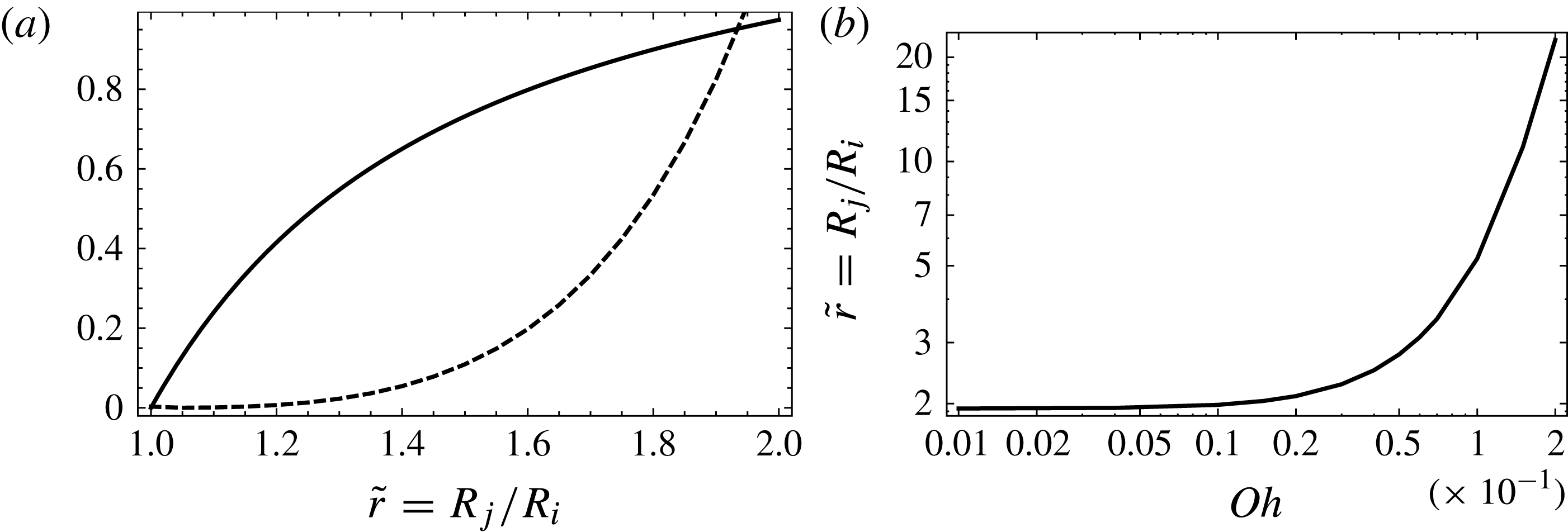
selected by the droplet-mediated jump creation. The integral (4.3) can be evaluated numerically using a simple trapezoidal integration of the profile computed with (2.14). In figure 11(a), we plot the left-hand side and the right-hand side of (4.4).
In figure 11(b), we show the dependence of the numerically computed ratio
 $\tilde{r}$
with respect to
 $\mathit{Oh}$
. The
 $R_{j}/R_{i}$
value tends to
 $1.934$
for small
 $\mathit{Oh}$
values. For liquid solutions I and II, we experimentally visited the ranges
 $0.01<\mathit{Oh}<0.02$
and
 $0.005<\mathit{Oh}<0.008$
, respectively, and the values of
 $R_{j}/R_{i}$
were measured to be 1.93 and 1.54, respectively. The small discrepancy can be explained by additional dissipative sources. In our model, the surface shear has been disregarded and this assumption might not be valid for all classes of surfactant, as described by Buzza, Lu & Cates (Reference Buzza, Lu and Cates1995). Given that the predicted value is obtained by integrating over the whole PB profile, with no free parameter, the agreement is very satisfactory.
For the highest values of
 $\mathit{Oh}$
, the selected
 $R_{j}/R_{i}$
value tends to be very high. Unfortunately this regime cannot be tested experimentally since no capillary jumps were observed for
 $Oh\geqslant 0.05$
(Cohen et al.
Reference Cohen, Fraysse, Rajchenbach, Argentina, Bouret and Raufaste2014). From that value of
 $Oh$
, the capillary jump geometry is broken and the comparison with the model is no longer possible. We add that our model cannot predict this transition since the geometry is prescribed to that of a capillary jump.
(a) Graphical determination of the selected ratio
 $\tilde{r}=R_{j}/R_{i}$
for
 $Oh=10^{-3}$
. The thick solid curve and the dashed curve are the left-hand side and right-hand side functions of (4.4), respectively. (b) Selected ratio
 $\tilde{r}$
as a function of the Ohnesorge number
 $\mathit{Oh}$
.
5. Conclusion
In this article, we have reported a new kind of hydraulic jump mediated by capillary forces, instead of gravity. We have proposed a simple model for describing this hydraulic jump propagating along a Plateau border. The physics at play is controlled through the Weber and Reynolds numbers. The analogy with hydraulic jumps is evidenced by the existence condition
 $\mathit{We}>1/2$
. The propagation velocity and the profile are predicted through an equation describing the dynamics of a damped nonlinear oscillator. A simple and original experimental design has been proposed and implemented, which made the observation of these capillary jumps possible. All the measurements agree with the predictions of the theoretical approach, and confirm its validity, although we have never observed the solitary wave predicted by the model for
 $\mathit{We}<1/2$
, probably due to a too high viscosity of the liquid solutions.
(a) Schematic of the cross-section of the Plateau border. The thick curves represent the liquid–air interfaces. The thick black arc is the parametrized interface defined by (A 1) and (A 2). (b) Three-dimensional sketch of the Plateau border defined with a hyperbolic tangent function for
 $R(z)$
.

Supplementary movies
Supplementary movies are available at http://dx.doi.org/10.1017/jfm.2014.717.
Appendix A
In this appendix, we compute the averaged mean curvature (i.e. the mean curvature averaged over the azimuthal coordinate for a given cross-section) of the Plateau border. In figure 12(a), we show the cross-section of the channel. The top interface is parametrized as an arc of a circle of radius
 $R(z)$
,
 $$\begin{eqnarray}\displaystyle x & = & \displaystyle R(z)\cos {\it\phi},\end{eqnarray}$$
 $$\begin{eqnarray}\displaystyle y & = & \displaystyle R(z)({\it\nu}-\sin {\it\phi}),\end{eqnarray}$$
 ${\it\phi}\in [{\rm\pi}/3,2{\rm\pi}/3]$
and
 ${\it\nu}=2/\sqrt{3}$
. The diagonalization of the Hessian matrix on this surface yields the mean curvature
 $$\begin{eqnarray}H_{g}=-\frac{R(z)(1-{\it\nu}\sin {\it\phi})R^{\prime \prime }(z)-(-2{\it\nu}\sin {\it\phi}+{\it\nu}^{2}+1)R^{\prime }(z)^{2}-1}{R(z)[({\it\nu}\sin {\it\phi}-1)^{2}R^{\prime }(z)^{2}+1]^{3/2}}.\end{eqnarray}$$
Clearly, the variation of
 $R(z)$
induces a dependence of the curvature on the angular variable, as evidenced in figure 12(b). This expression simplifies to
 $$\begin{eqnarray}\displaystyle H_{g} & = & \displaystyle \displaystyle \frac{1}{R(z)}+\frac{1}{3}[(3+2\sqrt{3})\sin {\it\phi}-3]R^{\prime \prime }(z)\end{eqnarray}$$
 $$\begin{eqnarray}\displaystyle & & \displaystyle \displaystyle +\,\frac{[-3(7+4\sqrt{3})\sin ^{2}{\it\phi}+(6+4\sqrt{3})\sin {\it\phi}+8\sqrt{3}+11]R^{\prime }(z)^{2}}{6R(z)}+\text{h.o.t.},\end{eqnarray}$$
 ${\it\phi}={\rm\pi}/3$
and
 ${\it\phi}=2{\rm\pi}/3$
and we finally get the averaged mean curvature within the small slope approximation:
 $$\begin{eqnarray}{\it\kappa}=\frac{1}{R(z)}+{\it\beta}_{1}R^{\prime \prime }(z)+{\it\beta}_{2}\frac{R^{\prime }(z)^{2}}{R(z)},\end{eqnarray}$$
where
 ${\it\beta}_{1}=(2\sqrt{3}-{\rm\pi})/{\rm\pi}\sim 0.103$
and
 ${\it\beta}_{2}=(3\sqrt{3}-{\rm\pi})/6{\rm\pi}\sim 0.109$
.



