3.1 Cases

The LES experiments are not crafted as a case study of a specific submesoscale regime, but rather as an idealization designed to expose the generic dynamics of cold filament frontogenesis and arrest. In nature, filaments are spatially anisotropic structures with length-to-width ratios $\gg 10$ , especially during the sharpening phase of frontogenesis. At the same time, filaments are active in the OBL where the energy containing scales of turbulence $\ell$ are of the order of the boundary-layer depth $h$ and less $1<\ell <100~\text{m}$ . The wide scale separation between turbulence and fronts, 1 m–10 km, poses a severe computational challenge as the LES horizontal domain and resolution need to be simultaneously large enough and fine enough to resolve crucial scale interactions. The computational box needs to be sufficiently wide so that the geostrophic currents generated by the density filament are realistic in scale and magnitude with the resulting low wavenumber turbulent motions unconstrained by the periodic boundary conditions. At high wavenumbers the resolution needs to be fine enough so that most of the OBL turbulence is resolved with only a small fraction of the flux carried by the SGS model near the water surface.

Thus, given the goals of the simulations and the large aspect ratio of typical filaments we adopt a 2-D $(x{-}z)$ model of a filament for our LES modelling. The choice of domain size is initially guided by the results in McWilliams et al. (Reference McWilliams, Gula, Molemaker, Renault and Shchepetkin2015) and finally by extensive flow visualization and analysis of LES solutions in boxes of varying horizontal dimensions $(L_{x},L_{y})$ . The down-front domain width $L_{y}$ proves to be an important choice as we find $L_{y}$ needs to be large enough to support surprising large-scale anisotropic turbulence (see § 5 and the linear stability analysis of McWilliams, Molemaker & Olafsdottir (Reference McWilliams, Molemaker and Olafsdottir2009b )). Our explorations, although not exhaustive, lead us to pick the domain $(L_{x},L_{y},H)=(12,4.5,-0.25)~\text{km}$ with discretization $(N_{x},N_{y},N_{z})=(8192,3072,256)\sim 6.5\times 10^{9}$ grid points. This corresponds to a uniform horizontal spacing $\unicode[STIX]{x0394}x=\unicode[STIX]{x0394}y=1.46~\text{m}$ . The vertical grid is smoothly stretched with finer resolution near the water surface $\unicode[STIX]{x0394}z=[0.5-1.68]~\text{m}$ ; the vertical spacing between neighbouring cells is increased by a constant stretching factor $K=\unicode[STIX]{x0394}z_{k+1}/\unicode[STIX]{x0394}z_{k}=1.0048$ , for $k=1,N_{z}$ . Given the filament alignment in the computational box, the coordinates $(x,y,z)$ are also referred to as (cross-front, down-front, vertical) directions.

The expectation is that CFF will depend on the wind magnitude and direction based on the LES results for warm fronts described by Hamlington et al. (Reference Hamlington, Van Roekel, Fox-Kemper, Julien and Chini2014) and Suzuki et al. (Reference Suzuki, Fox-Kemper, Hamlington and Roekel2016). In the present work with cold filaments, the external forcing of the OBL is by surface winds or by surface cooling. Wind stress is applied in either the west-to-east or south-to-north directions with a water side friction velocity $u_{\ast }=0.01~\text{m}~\text{s}^{-1}$ with zero surface cooling $Q_{\ast }$ . This corresponds to surface winds of $U=8.5~\text{m}~\text{s}^{-1}$ with a drag coefficient $C_{d}\sim 1.2\times 10^{-3}$ based on the relationship given by Large & Pond (Reference Large and Pond1981). To examine the robustness of our findings, we consider a third simulation with $u_{\ast }=0$ and a finite surface cooling of $100~\text{W}~\text{m}^{-2}$ , which equates to a kinematic surface flux $Q_{\ast }=2.38\times 10^{-5}~\text{K}~\text{m}^{-1}~\text{s}^{-1}$ . Later, turbulence quantities are normalized by $(u_{\ast },w_{\ast })$ in the non-zero (wind, cooling) cases, respectively. The Deardorff (Reference Deardorff1972a ) convective velocity scale is $w_{\ast }=(\unicode[STIX]{x1D6FD}|h_{i}|Q_{\ast })^{1/3}$ , where $h_{i}=-66.5~\text{m}$ is the initial OBL depth before the submesoscale filament is introduced (§ 3.3). The velocity scales of the external forcing are used to normalize the velocities since the properties of the imposed filament are identical across the simulations. In all simulations the Coriolis parameter $f=7.81\times 10^{-5}~\text{s}^{-1}$ . To streamline the discussion the following acronyms are introduced: $E$ denotes the simulation with west-to-east (or cross-front) winds, $N$ denotes the simulation with south-to-north (or down-front) winds and $C$ denotes the simulation driven by surface cooling. Table 1 provides a summary of the simulations and selected bulk statistics.

Table 1.

Simulations and bulk properties. In the table, $(t_{m},x_{p}/L,\text{TKE})$ are the (time stamp, cross-front location, TKE) where $\langle \unicode[STIX]{x1D701}\rangle _{p}$ reaches its maximum value. Turbulent kinetic energy (TKE) for $(E,N,C)$ is normalized by $(u_{\ast }^{2},u_{\ast }^{2},w_{\ast }^{2})$ , respectively.

Among the possible instabilities for submesoscale fronts and filaments is the so-called mixed layer instability (MLI; Boccaletti et al. Reference Boccaletti, Ferrari and Fox-Kemper2007; Fox-Kemper et al. Reference Fox-Kemper, Ferrari and Hallberg2008). MLI is a variant of Eady’s classical baroclinic instability problem with uniform mean stratification $N_{ML}$ and mean vertical shear $\text{d}V/\text{d}z$ , and its most unstable eigenmodes have a horizontal scale near the mixed layer deformation radius, $R_{ML}=N_{ML}H_{ML}/f$ . In interpreting its relevance to a continuously stratified fluid with vertical profile $N(z)$ , the estimation of $N_{ML}$ is somewhat ambiguous. In our far-field initial conditions at $t=2~\text{h}$ (§ 5.1), $H_{ML}=66~\text{m}$ , and the $N$ values in the middle of the mixed layer or at the bottom in the upper pycnocline are less than 0.3 or $7\times 10^{-3}~\text{s}^{-1}$ , respectively; the corresponding $R_{ML}$ estimates are less than 0.2 or 6 km, respectively. Also the fastest growing MLI time scale using equation (3) of Fox-Kemper et al. (Reference Fox-Kemper, Ferrari and Hallberg2008) gives an e-folding scale of 14.6 h which is long compared to the 15 h of simulation considered here. Thus, the posing of our problems here with $(L_{x},L_{y})=(12,4.5)~\text{km}$ is at least marginally large enough to resolve an active MLI mode if one were to arise in the more complicated filament flow field and active boundary-layer turbulent mixing in our simulations; yet we see no evidence of MLI in our solutions with its signature of $\langle w^{\prime }b^{\prime }\rangle >0$ , see §§ 5.3 and 5.4.

3.2 Thermal wind

The structure of the mean buoyancy field and the resulting geostrophic pressure gradients (thermal wind) used in the LES follow the design outlined by McWilliams et al. (Reference McWilliams, Gula, Molemaker, Renault and Shchepetkin2015). Given a 2-D buoyancy field $b(x,z)$ , the interior companion mean geostrophic shear profile is (e.g. Gill Reference Gill1982)

(3.1) $$\begin{eqnarray}\boldsymbol{s}_{g}(x,z)=\frac{1}{f}\hat{\boldsymbol{z}}\times \unicode[STIX]{x1D735}_{\bot }b,\end{eqnarray}$$

where the subscript $\bot$ denotes a horizontal vector in the $(x,y)$ plane. Then the geostrophic current $\boldsymbol{u}_{g}=(0,v_{g})$ is

(3.2) $$\begin{eqnarray}\boldsymbol{u}_{g}(x,z)=\int _{H}^{z}\boldsymbol{s}_{g}\,\text{d}z^{\prime }\end{eqnarray}$$

taking the current deep in the water $\boldsymbol{u}_{g}(z=H)=0$ .

In our prescription of the buoyancy, its cross-front variation at the water surface $z=0$ is the smooth function $b_{s}(x)=b_{o}-\unicode[STIX]{x1D6FF}b_{o}\exp [-(x/L)^{2}]$ , where $b_{o}$ is a constant background value, $\unicode[STIX]{x1D6FF}b_{o}$ is the buoyancy jump, $L$ is the front scale and $x=0$ is the location of the front centreline. Given the cross-front length $L_{x}=12~\text{km}$ of our computational box, we choose $(\unicode[STIX]{x1D6FF}b_{o},L)=$  ( $0.785\times 10^{-3}~\text{m}~\text{s}^{-2}$ , 2 km) as a compromise between realism and computational cost. These values result in a temperature jump of 0.48 K across a symmetric front of width $2L=4~\text{km}$ with maximum and minimum geostrophic currents $\pm 0.25~\text{m}~\text{s}^{-1}$ . Further details of the buoyancy field specification in the OBL interior are given in the appendix A.

3.3 Turbulent filament initialization

A multi-step recipe is used to initialize the filament simulations. First, simulations are started with the frontal parameters set to zero with turbulence triggered by small random perturbations to the buoyancy and current fields. Essentially, these pre-front LES are simulations of a spatially homogeneous OBL in a very large horizontal domain with wind stress or cooling either on or off from the outset depending on the desired attributes of the final frontal simulation. The simulations are integrated for more than 30 physical hours, in terms of a non-dimensional time $T=tu_{\ast }/|h|>20$ , which leads to well-developed turbulence. Statistics from the pre-front simulations are in good agreement with previous results, e.g. McWilliams et al. (Reference McWilliams, Sullivan and Moeng1997), Sullivan et al. (Reference Sullivan, Romero, McWilliams and Melville2012). Vertical profiles of the average horizontal currents $(\overline{u},\overline{v})$ are shown in figure 1. Here the averaging is over horizontal planes and over the time interval $25<t<30~\text{h}$ ; this averaging differs from that used in the presence of a filament (§ 4).

Figure 1.

Average currents from the homogeneous (pre-front) runs used to initialize the simulations with cold filaments. $(\overline{u},\overline{v})/u_{\ast }$ are indicated by (red, black) colours. The (solid lines, open circles) are current profiles obtained for $(E,N)$ winds, respectively. The mixed layer depth $h_{i}=-66.5~\text{m}$ . Because of the rotational symmetry of the horizontally homogeneous problem, $(\overline{u},\overline{v})$ from $E$ equals $(\overline{v},-\overline{u})$ from $N$ . These profiles are obtained by averaging over complete horizontal $x{-}y$ planes and by averaging over five hours. For clarity the open circles are shown at every second grid level for case $N$ . The horizontal currents for the cooling simulation $C$ are zero (not shown).

Next, the last volume from the pre-front simulations serves as the restart volume for the frontal calculations with the following modifications. First, the mean buoyancy field in the restart volume is replaced with the three-layer horizontal and mean vertical frontal structure $b(x,z)$ given by (A 1). A three-dimensional buoyancy field is then generated by adding the turbulent buoyancy fluctuations from the restart volume to $b(x,z)$ . This modified restart volume contains realistic turbulent fields plus the desired mean buoyancy field, however, it is lacking secondary circulations and in particular the central downwelling current, which is a key feature initiating frontogenesis. To stimulate secondary circulations, the simulations are next integrated forward in time holding the frontal buoyancy field fixed until a downwelling jet develops, this avoids slumping of the buoyancy field. We monitor the motions near the thermocline and find a vigorous downwelling jet and secondary circulations develop after approximately 1.8 h. Finally, at this point in the initialization all fields are allowed to evolve freely in time. The subsequent analysis references this special time as $t=0~\text{h}$ . Thus the initial conditions for our frontal calculations are more complete than the thermal wind (geostrophic) balance used by Skyllingstad & Samelson (Reference Skyllingstad and Samelson2012) and Hamlington et al. (Reference Hamlington, Van Roekel, Fox-Kemper, Julien and Chini2014) who superimpose frontal structures on top of an initially laminar flow. In the mixed layer, the initial state of our LES is an unsteady analogue to the TTW balance described by McWilliams et al. (Reference McWilliams, Gula, Molemaker, Renault and Shchepetkin2015) as the fields contain fully developed resolved turbulence and secondary circulations (e.g. figure 3 and the discussion in § 5.1). The simulations are integrated for more than 20 h past the start time $t=0$ .

In terms of the turbulent velocity scales $(u_{\ast },w_{\ast })$ based on the surface wind and buoyancy forcing that we use for normalizing the simulation results (as conventional in boundary-layer turbulence), the initial geostrophic velocity maximum is 15–20 times larger.

4.1 Down-front average equations

Applying $y$ averaging to the momentum and buoyancy equations (2.1a ) and (2.1b ), decomposing the flow fields according to the prescription (4.1), and invoking the averaging rule given by (4.2) leads to the equation set:

(4.3a ) $$\begin{eqnarray}\displaystyle \frac{\unicode[STIX]{x2202}}{\unicode[STIX]{x2202}t}\langle u\rangle & = & \displaystyle -\frac{\unicode[STIX]{x2202}}{\unicode[STIX]{x2202}x}(\langle u\rangle \langle u\rangle +\langle u^{\prime }u^{\prime }\rangle +\frac{\langle p\rangle }{\unicode[STIX]{x1D70C}_{o}}+\frac{2\langle e\rangle }{3}+\langle \unicode[STIX]{x1D70F}_{11}\rangle )\nonumber\\ \displaystyle & & \displaystyle -\,\frac{\unicode[STIX]{x2202}}{\unicode[STIX]{x2202}z}(\langle u\rangle \langle w\rangle +\langle u^{\prime }w^{\prime }\rangle +\langle \unicode[STIX]{x1D70F}_{13}\rangle )+f\langle v\rangle ,\end{eqnarray}$$

(4.3b ) $$\begin{eqnarray}\displaystyle \frac{\unicode[STIX]{x2202}}{\unicode[STIX]{x2202}t}\langle v\rangle & = & \displaystyle -\frac{\unicode[STIX]{x2202}}{\unicode[STIX]{x2202}x}(\langle u\rangle \langle v\rangle +\langle u^{\prime }v^{\prime }\rangle +\langle \unicode[STIX]{x1D70F}_{12}\rangle )\nonumber\\ \displaystyle & & \displaystyle -\,\frac{\unicode[STIX]{x2202}}{\unicode[STIX]{x2202}z}(\langle v\rangle \langle w\rangle +\langle v^{\prime }w^{\prime }\rangle +\langle \unicode[STIX]{x1D70F}_{23}\rangle )-f\langle u\rangle ,\end{eqnarray}$$

(4.3c ) $$\begin{eqnarray}\displaystyle \frac{\unicode[STIX]{x2202}}{\unicode[STIX]{x2202}t}\langle w\rangle & = & \displaystyle -\frac{\unicode[STIX]{x2202}}{\unicode[STIX]{x2202}x}(\langle u\rangle \langle w\rangle +\langle u^{\prime }w^{\prime }\rangle +\langle \unicode[STIX]{x1D70F}_{13}\rangle )\nonumber\\ \displaystyle & & \displaystyle -\,\frac{\unicode[STIX]{x2202}}{\unicode[STIX]{x2202}z}\left(\langle w\rangle \langle w\rangle +\langle w^{\prime }w^{\prime }\rangle +\langle \unicode[STIX]{x1D70F}_{33}\rangle +\frac{\langle p\rangle }{\unicode[STIX]{x1D70C}_{o}}+\frac{2\langle e\rangle }{3}\right)+\langle b\rangle ,\end{eqnarray}$$

(4.3d ) $$\begin{eqnarray}\displaystyle \frac{\unicode[STIX]{x2202}}{\unicode[STIX]{x2202}t}\langle b\rangle & = & \displaystyle -\frac{\unicode[STIX]{x2202}}{\unicode[STIX]{x2202}x}(\langle u\rangle \langle b\rangle +\langle u^{\prime }b^{\prime }\rangle +\langle \unicode[STIX]{x1D70F}_{1b}\rangle )\nonumber\\ \displaystyle & & \displaystyle -\,\frac{\unicode[STIX]{x2202}}{\unicode[STIX]{x2202}z}(\langle w\rangle \langle b\rangle +\langle w^{\prime }b^{\prime }\rangle +\langle \unicode[STIX]{x1D70F}_{3b}\rangle ).\end{eqnarray}$$

$x$

$z$

$x{-}y$

$\langle w\rangle =0$

5.1 Initial mean circulations and TTW

Our interpretation of the LES solutions begins with a discussion of the average flow fields at $t=2~\text{h}$ . Adopting a TTW approximation (Gula et al. Reference Gula, Molemaker and McWilliams2014; McWilliams et al. Reference McWilliams, Gula, Molemaker, Renault and Shchepetkin2015), the $x{-}z$ spatial distribution of horizontal and vertical currents in our LES is approximately described by the balance between pressure gradients, Coriolis force and divergence of turbulent momentum fluxes:

(5.1a ) $$\begin{eqnarray}\displaystyle & \displaystyle f\langle v\rangle \approx \frac{\unicode[STIX]{x2202}}{\unicode[STIX]{x2202}x}\frac{\langle p\rangle }{\unicode[STIX]{x1D70C}_{o}}+\frac{\unicode[STIX]{x2202}}{\unicode[STIX]{x2202}z}(\langle u^{\prime }w^{\prime }\rangle +\langle \unicode[STIX]{x1D70F}_{13}\rangle ), & \displaystyle\end{eqnarray}$$

(5.1b ) $$\begin{eqnarray}\displaystyle & \displaystyle f\langle u\rangle \approx -\frac{\unicode[STIX]{x2202}}{\unicode[STIX]{x2202}z}(\langle v^{\prime }w^{\prime }\rangle +\langle \unicode[STIX]{x1D70F}_{23}\rangle ), & \displaystyle\end{eqnarray}$$

(5.1c ) $$\begin{eqnarray}\displaystyle & \displaystyle \frac{\unicode[STIX]{x2202}\langle w\rangle }{\unicode[STIX]{x2202}z}\approx -\frac{\unicode[STIX]{x2202}\langle u\rangle }{\unicode[STIX]{x2202}x}. & \displaystyle\end{eqnarray}$$

Figure 3.

Average fields at $t=2~\text{h}$ for simulation $E$ . The fields displayed from top to bottom are temperature $\langle \unicode[STIX]{x1D703}-\unicode[STIX]{x1D703}_{o}\rangle$ with the colour bar in K, followed by down-front velocity $\langle v\rangle$ , cross-front velocity $\langle u\rangle$ and vertical velocity $\langle w\rangle$ . In the far field the $\langle u(x,z),v(x,z)\rangle$ currents are equivalent to the homogeneous currents for the east wind shown in figure 1. Colour bars for the velocity fields are in units of $\text{m}~\text{s}^{-1}$ . The averaging operator $\langle \cdot \rangle$ is defined in § 5, and the $\unicode[STIX]{x1D703}$ nudging, described in § 3.3, has been applied for 1.8 h before $t=2$ . For clarity, contour lines of $\langle w\rangle$ are not shown in figures 3(d), 4(d) and 5(d).

Figure 4.

Average fields at $t=2~\text{h}$ for simulation $N$ . The fields displayed from top to bottom are temperature $\langle \unicode[STIX]{x1D703}-\unicode[STIX]{x1D703}_{o}\rangle$ with the colour bar in K, followed by down-front velocity $\langle v\rangle$ , cross-front velocity $\langle u\rangle$ and vertical velocity $\langle w\rangle$ . In the far field the $\langle u(x,z),v(x,z)\rangle$ currents are equivalent to the homogeneous currents for the north wind shown in figure 1. Colour bars for the velocity fields are in units of $\text{m}~\text{s}^{-1}$ .

Figure 5.

Average fields at $t=2~\text{h}$ for simulation $C$ . The fields displayed from top to bottom are temperature $\langle \unicode[STIX]{x1D703}-\unicode[STIX]{x1D703}_{o}\rangle$ with the colour bar in K, followed by down-front velocity $\langle v\rangle$ , cross-front velocity $\langle u\rangle$ and vertical velocity $\langle w\rangle$ . The fields are symmetric about $x=0$ within sampling error. In the far field the currents $\langle u(x,z),v(x,z)\rangle =0$ match the average currents for a homogeneous OBL driven by surface cooling. Colour bars for the velocity fields are in units of $\text{m}~\text{s}^{-1}$ .

Snapshots of the average flow fields in an $x{-}z$ plane for simulations $(E,N,C)$ are shown in figures 3–5, respectively. The visualization depicts the main features of the initialization: a cold dense filament of total width $2L\sim 4~\text{km}$ fills the boundary layer to a depth of ${\sim}-66~\text{m}$ . The density anomaly is partly balanced by down-front currents $\langle v\rangle$ with large (negative, positive) side lobes (left, right) of the front centreline $x=0$ . Secondary currents $\langle u,w\rangle$ develop in the boundary layer that feature a broad central downwelling jet with weaker upwelling in the far field with opposing cross-front branches left and right of the front centreline in the surface layer. Also, figures 3 and 4 show significant asymmetry in the horizontal currents and temperature field about the filament centreline because of wind forcing. The vertical velocity $w$ is well resolved in the LES but its fluctuations $w^{\prime }$ vary rapidly over small scales with amplitude nearly 10 times $\langle w\rangle$ . Thus the apparent ‘noise’ in figures 3(d), 4(d), 5(d) is simply random error resulting from limited down-front $y$ averaging. These small-scale fluctuations are damped by averaging over an even wider $y$ domain.

Secondary circulations (or cells) are a key staple of TTW and significantly influence our interpretation of frontogenetic evolution with OBL turbulence. They can be inferred from the secondary currents $\langle u,w\rangle$ , but to identify them more clearly in our simulations we present contours of the non-divergent ageostrophic two-dimensional streamfunction $\unicode[STIX]{x1D713}$ computed from $\langle u\rangle$ for the different simulations at $t=2~\text{h}$ in figures 6(a), 7(a), and 8(a). Here

(5.2) $$\begin{eqnarray}\unicode[STIX]{x1D713}(x,z)=\int _{H}^{z}\langle u\rangle (x,z^{\prime })\,\text{d}z^{\prime },\end{eqnarray}$$

with the lower boundary condition $\unicode[STIX]{x1D713}(x,H)=0$ . It is now readily apparent that as part of the turbulent filament initialization a pair of coherent SC emerge (left, right) of the filament centreline at $t=2~\text{h}$ independent of the external forcing. Because the cross-front $\langle u\rangle$ current is an order of magnitude larger than the downwelling $\langle w\rangle$ current, combined with the wide horizontal and thin vertical scales, the rotational pattern of the secondary circulations take on a vertically thin elliptical shape.

Figure 6.

Contours of the two-dimensional ageostrophic overturning streamfunction $\unicode[STIX]{x1D713}$ in the $x{-}z$ plane computed from the average velocity $\langle u\rangle$ at three different time stamps for the simulation with cross-front winds $E$ . $t=2~\text{h}$ (a), $t_{m}=4.50~\text{h}$ time of maximum vertical vorticity (b), $t=9~\text{h}$ a late time past the peak vorticity (c). In (a) the horizontal vectors indicate the flow direction at the top of the secondary circulation. The colour bar is in units of $\text{m}^{2}\text{s}^{-1}$ .

Figure 7.

Contours of the two-dimensional ageostrophic overturning streamfunction $\unicode[STIX]{x1D713}$ in the $x{-}z$ plane as in figure 6 but for the simulation with down-front winds $N$ . $t=2~\text{h}$ (a), $t_{m}=5.02~\text{h}$ time of maximum vertical vorticity (b), $t=9~\text{h}$ a late time past the peak vorticity (c). The colour bar is in units of $\text{m}^{2}\text{s}^{-1}$ .

Figure 8.

Contours of the two-dimensional ageostrophic overturning streamfunction $\unicode[STIX]{x1D713}$ in the $x{-}z$ plane as in figure 6 but for the simulation driven by surface cooling $C$ . $t=2~\text{h}$ (a), $t_{m}=6.13~\text{h}$ time of maximum vertical vorticity (b), $t=9~\text{h}$ a late time past the peak vorticity. The colour bar is in units of $\text{m}^{2}\text{s}^{-1}$ .

It is important to notice that the amplitude and streamline pattern of the secondary circulations with surface cooling (no wind stress), shown in figures 5 and 8, are qualitatively similar to those in $(E,N)$ . Remarkably, starting from fully developed (convective) turbulence with no net vertical momentum flux in $C$ , a coherent secondary circulation and non-zero resolved turbulent vertical momentum fluxes $\langle u^{\prime }w^{\prime },v^{\prime }w^{\prime }\rangle$ are generated by turbulence–filament interactions as shown in figure 9. With no wind stress, these fluxes approach zero at $z=0$ and are odd-symmetric about the filament centreline. The maximum absolute values occur in the upper OBL, near $z\sim -20~\text{m}$ and are noticeably offset left and right of $x=0$ . For $z>-20~\text{m}$ the divergence $-\unicode[STIX]{x2202}_{z}\langle v^{\prime }w^{\prime }\rangle$ generates (positive, negative) secondary $u$ currents on the (left, right) sides of the filament centreline according to (5.1b ); also see figures 5 and 9. Thus, near the water surface turbulent momentum fluxes generate converging $u$ currents at the filament centreline. For $z<-20~\text{m}$ , the divergence $-\unicode[STIX]{x2202}_{z}\langle v^{\prime }w^{\prime }\rangle$ changes sign causing the cross-front currents to flow away from the filament centreline. The cross-front flux $\langle u^{\prime }w^{\prime }\rangle$ is smaller in amplitude compared to its down-front counterpart, and the flux divergence $\unicode[STIX]{x2202}_{z}\langle u^{\prime }w^{\prime }\rangle$ tends to oppose the geostrophic current $v_{g}$ on either side of the filament; hence turbulence re-enforces the imbalance $\langle v\rangle \neq v_{g}$ . The spatial pattern of $\langle w\rangle (x,z)$ follows from (5.1c ). At $t=2~\text{h}$ , the spatial distribution of $\langle u^{\prime }w^{\prime },v^{\prime }w^{\prime }\rangle$ for $(E,N)$ are qualitatively similar to those in $C$ (not shown).

Figure 9.

Resolved turbulent fluxes $\langle u^{\prime }w^{\prime }\rangle$ (a) and $\langle v^{\prime }w^{\prime }\rangle$ (b) from simulation $C$ at $t=2~\text{h}$ . Fluxes are normalized by $w_{\ast }^{2}$ , and the colour bar is in non-dimensional units. A vertical profile of the turbulent flux averaged between $-250<x<-600~\text{m}$ (solid lines) and $250>x>600~\text{m}$ (dashed lines) is shown in the right frame. The fluxes on the right side of the front are multiplied by $-$ 1 to better compare with the left side.

Within sampling error, the $\langle \boldsymbol{u},\unicode[STIX]{x1D703}\rangle$ fields in the cooling simulation $C$ display appropriate odd–even symmetries about $x=0$ , i.e.  $\langle u,v\rangle$ are odd functions while $\langle w,\unicode[STIX]{x1D703}\rangle$ are even functions. In contrast, in the simulations with cross-front and down-front winds $(E,N)$ the magnitudes and patterns of the $\langle u,v\rangle$ currents are noticeably asymmetrical, exhibiting a wind direction dependence about the filament centreline. To a first approximation this broken symmetry can be understood as a superposition of secondary circulations, as in $C$ , and Ekman boundary-layer currents (see also McWilliams et al. Reference McWilliams, Gula, Molemaker, Renault and Shchepetkin2015). To expand on this idea, consider the horizontal mean currents $(\overline{u},\overline{v})$ in figure 1 from our spatially homogeneous boundary layers used to initiate the frontal simulations. Inspection of these curves shows the expected results for a homogeneous OBL (e.g. McWilliams et al. Reference McWilliams, Sullivan and Moeng1997). With cross-front winds the Ekman $\overline{v}$ current is negative, rotated to the right of the wind and decays monotonically with depth. Meanwhile, its companion Ekman $\overline{u}$ current spirals with depth; $\overline{u}$ is positive and surface intensified for $0>z>0.25h$ but crosses over to negative values near $z\sim 0.25h$ so that the bulk integral $\int \overline{u}\,\text{d}z=0$ . Both $(\overline{u},\overline{v})$ decay to zero near $h$ . Because of symmetries in the forcing, $(\overline{v},-\overline{u})$ for $N$ $=$ $(\overline{u},\overline{v})$ for $E$ .

Further comparison of the streamfunction patterns in figures 6 and 7 shows cross-front Ekman transport in the far field away from the filament in $(E,N)$ especially in the down-front wind simulation. However, near the filament the coherent cells significantly modify the Ekman flow. In $N$ , the secondary circulations are slightly offset vertically with the cell centre on the right-hand side lying closer to the water surface. Apparently the boundary-layer Ekman flow and secondary circulations work constructively/destructively on the left-/right-hand side of the filament. It is interesting to trace the complex trajectory of near-surface streamlines in the down-front wind simulation. For example, on the far left-hand side of the domain near $z\sim -25~\text{m}$ the streamlines are initially squeezed in the vertical direction as they approach the filament centre, a consequence of the enhanced $u$ current in the secondary circulations. Then the streamlines smoothly cross the filament axis, dive deep into the boundary layer tracking out a trajectory below the secondary circulations on the right-hand side and finally re-surface well to the east of the secondary circulation. Notice that in the region $0<x<3000~\text{m}$ , the cross-front flow is near zero or slightly negative in the upper boundary layer, i.e. the return current from the secondary circulation blocks the cross-front Ekman boundary-layer transport, also see figure 10. In the $E$ case, the boundary-layer $v$ current favours/opposes the geostrophic current $v_{g}$ left/right of $x=0$ over the entire mixed layer. At the same time, the boundary-layer $u$ current acts in a differential manner, it (strengthens, weakens) the secondary $u$ circulation in the surface layer, but has an opposite effect below $z<0.25h$ .

Figure 10.

Average currents $\langle u,v\rangle$ indicated by (red, blue) lines (a–c), and average temperature $\langle \unicode[STIX]{x1D703}-\unicode[STIX]{x1D703}_{o}\rangle$ (d–f) near the water surface $0<-z<5~\text{m}$ . Profiles are shown at $t=0~\text{h}$ (dotted lines) and time $t_{m}$ where the peak vertical vorticity $\langle \unicode[STIX]{x1D701}\rangle _{p}$ is a maximum (solid lines). The currents in simulations $(E,N,C)$ are normalized by $(u_{\ast },u_{\ast },w_{\ast })$ , respectively, and the temperature is normalized by the temperature jump between the far field and the filament centre $|\unicode[STIX]{x1D6FF}\unicode[STIX]{x1D703}_{o}|=0.48~\text{K}$ (see appendix A).

Figure 11.

Average fluxes $\langle u\rangle \langle u\rangle$ (a,b) and $\langle u\rangle \langle v\rangle$ (c,d) for simulations $(E,N,C)$ , indicated by (blue, black, red) lines, respectively. (a,c) Compare results at $t=0$ and (b,d) at the time of maximum $\langle \unicode[STIX]{x1D701}\rangle _{p}$ . Fluxes in simulations $(E,N,C)$ are normalized by $(u_{\ast }^{2},u_{\ast }^{2},w_{\ast }^{2})$ , respectively.

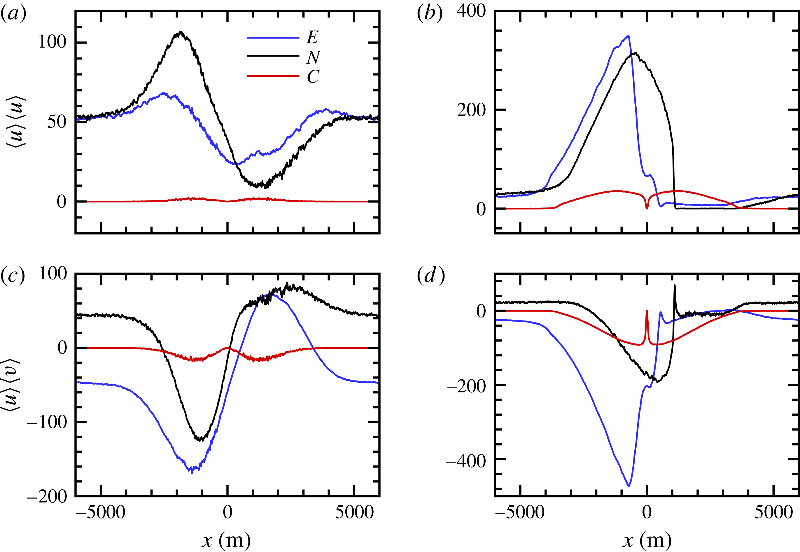
The mean currents $\langle u,v\rangle$ and their momentum fluxes in a near-surface layer of depth $-5<z<0~\text{m}$ at $t=0$ are presented as line plots in figures 10 and 11; they add further support to our interpretation of the streamfunction patterns. Because $\langle u\rangle \langle u\rangle$ and $\langle u\rangle \langle v\rangle$ are nonlinear products the mean current fluxes are even more strongly asymmetrical functions about $x=0$ with notably bigger amplitude compared to the currents; consequently the cross-front $x$ divergence and time tendencies in (4.3) are also larger on the left side of the filament. The imbalances between the left and right sides at $t=0$ hold, independent of the wind direction $E$ or $N$ , because each involves some Ekman flow from west to east. The asymmetry, of course, would be shifted to the right side of a filament for an east-to-west cross-front wind or a north-to-south down-front wind.

The constructive–destructive superposition of the Ekman flow and secondary circulations has important consequences. Because of the competing effects, the horizontal buoyancy flux is asymmetrical but directed inwards from both filament edges towards the cool filament centre, i.e. the boundary layer re-stratifies from both edges. The mean transport of warm water is strong/weak from the left/right filament edges. This is an opposite result compared to the findings reported by Thomas & Lee (Reference Thomas and Lee2005), Skyllingstad & Samelson (Reference Skyllingstad and Samelson2012), Thomas et al. (Reference Thomas, Ferrari and Joyce2013), Hamlington et al. (Reference Hamlington, Van Roekel, Fox-Kemper, Julien and Chini2014) and others who find that their filament edges are stable and unstable because of Ekman buoyancy flux for weak warm filaments. From a stratification perspective, the turbulent flow near the water surface is in a weakly stable (left side) or marginally stable (right side) regime because of the vigorous secondary circulations induced by turbulence at $t=0$ . Potent SC inhibit convective overturning at a filament edge and thus fundamentally alter the type of instability that leads to arrest and decay in cold filament frontogenesis driven by cross-front or down-front winds or surface cooling, see §§ 5.2 and 5.3.

A scaling estimate of the competition between Ekman buoyancy flux and the TTW SC can be made based on the estimates in McWilliams (Reference McWilliams2017). For an Ekman layer depth comparable to the mixed layer depth (figure 1), the cross-front Ekman velocity ${\sim}u_{\ast }^{2}/f|h|$ , while the linear TTW balance velocity is ${\sim}\unicode[STIX]{x1D708}_{v}v_{g}/fh^{2}$ , where $h$ is the mixed layer depth, $v_{g}$ is the geostrophic down-front velocity, and $\unicode[STIX]{x1D708}_{v}$ is the diagnosed vertical eddy viscosity, $-\langle \boldsymbol{u}^{\prime }\boldsymbol{w}^{\prime }\rangle \cdot \unicode[STIX]{x2202}_{z}\langle \boldsymbol{u}\rangle /(\unicode[STIX]{x2202}_{z}\langle \boldsymbol{u}\rangle )^{2}$ . With characteristic values of $u_{\ast }=0.01~\text{m}~\text{s}^{-1}$ , $f=0.9\times 10^{-4}~\text{s}^{-1}$ , $h=-70~\text{m}$ , $v_{g}=0.25~\text{m}~\text{s}^{-1}$ and $\unicode[STIX]{x1D708}_{v}=0.1~\text{m}^{2}~\text{s}^{-1}$ , the Ekman velocity estimate is ${\approx}0.02~\text{m}~\text{s}^{-1}$ , while the TTW velocity estimate is a larger value of ${\approx}0.06~\text{m}~\text{s}^{-1}$ . Thus, for stronger frontal velocity and turbulent mixing and weaker wind stress, the SC can block Ekman buoyancy flux, as in the cases here (figures 6–8), even when the wind is down-front (case N) and the Ekman transport is nominally across the front (case N). In general because of SC the standard (far-field) 1-D Ekman momentum and volume transport balances do not hold near the filament.

Another widely discussed feature of a down-front wind is an extraction of potential vorticity by the surface stress and vertical momentum mixing, leading to negative potential vorticity, symmetric (or centrifugal) instability and enhanced turbulence (Thomas Reference Thomas2005; Taylor & Ferrari Reference Taylor and Ferrari2009). Figure 12 shows the Ertel potential vorticity associated with the $y$ -averaged fields,

(5.3) $$\begin{eqnarray}\langle q\rangle =\left(\,f+\frac{\unicode[STIX]{x2202}\langle v\rangle }{\unicode[STIX]{x2202}x}\right)\frac{\unicode[STIX]{x2202}\langle b\rangle }{\unicode[STIX]{x2202}z}-\frac{\unicode[STIX]{x2202}\langle v\rangle }{\unicode[STIX]{x2202}z}\frac{\unicode[STIX]{x2202}\langle b\rangle }{\unicode[STIX]{x2202}x},\end{eqnarray}$$

at $t=2~\text{h}$ for all three cases. As expected $\langle q\rangle$ is smaller in the boundary layer than in the pycnocline below. The action of turbulent overturning motions and entrainment is also evident at the base of the boundary layer. Case $N$ is distinguished by a modestly negative region near the surface under the northward jet (i.e. the one with a down-front wind). This confirms the expected potential vorticity extraction and sets up a sufficient condition for linear, inviscid symmetric instability. However, the latter is not clearly evident in our case $N$ simulation, implying that the other sources of turbulence are dominant here and perhaps that strong mixing inhibits its occurrence. As frontogenesis proceeds even this degree of $\langle q\rangle <0$ abates in all three cases.

Figure 12.

Average potential vorticity (PV) estimated from (5.3) at $t=2~\text{h}$ for cases $(E,N,C)$ shown in panels (a–c), respectively. The colour bar for PV is in units of $\text{s}^{-3}\times 10^{8}$ .

5.2 Frontogenetic progression

Section 5.1 shows that in the onset phase a coherent secondary circulation develops and persists in the LES against a background of fully developed OBL turbulence. A next step is then to examine the impact of fully resolved turbulent momentum and buoyancy fluxes on the sharpening of the cross-filament buoyancy and horizontal velocity gradients and the evolution of secondary circulations. To describe the dynamics of frontogenesis beyond $t>2~\text{h}$ we need to include time tendency and cross-front divergences in (4.3) in our discussion. Assuming fine grids and hence small SGS contributions, the important new terms to consider are then the following:

(5.4a ) $$\begin{eqnarray}\displaystyle & \displaystyle \frac{\unicode[STIX]{x2202}}{\unicode[STIX]{x2202}t}\langle u\rangle \sim -\frac{\unicode[STIX]{x2202}}{\unicode[STIX]{x2202}x}(\langle u\rangle \langle u\rangle +\langle u^{\prime }u^{\prime }\rangle )+\cdots \,, & \displaystyle\end{eqnarray}$$

(5.4b ) $$\begin{eqnarray}\displaystyle & \displaystyle \frac{\unicode[STIX]{x2202}}{\unicode[STIX]{x2202}t}\langle v\rangle \sim -\frac{\unicode[STIX]{x2202}}{\unicode[STIX]{x2202}x}(\langle u\rangle \langle v\rangle +\langle u^{\prime }v^{\prime }\rangle )+\cdots \,, & \displaystyle\end{eqnarray}$$

(5.4c ) $$\begin{eqnarray}\displaystyle & \displaystyle \frac{\unicode[STIX]{x2202}}{\unicode[STIX]{x2202}t}\langle w\rangle \sim -\frac{\unicode[STIX]{x2202}}{\unicode[STIX]{x2202}x}(\langle u\rangle \langle w\rangle +\langle u^{\prime }w^{\prime }\rangle )+\cdots \,, & \displaystyle\end{eqnarray}$$

(5.4d ) $$\begin{eqnarray}\displaystyle & \displaystyle \frac{\unicode[STIX]{x2202}}{\unicode[STIX]{x2202}t}\langle b\rangle \sim -\frac{\unicode[STIX]{x2202}}{\unicode[STIX]{x2202}x}(\langle u\rangle \langle b\rangle +\langle u^{\prime }b^{\prime }\rangle )+\cdots \,. & \displaystyle\end{eqnarray}$$

The lifecycle of frontal onset, arrest and decay in our simulations $(E,N,C)$ is demonstrated in figure 2. Here we follow Capet et al. (Reference Capet, McWilliams, Molemaker and Shchepetkin2008), Gula et al. (Reference Gula, Molemaker and McWilliams2014) and McWilliams et al. (Reference McWilliams, Gula, Molemaker, Renault and Shchepetkin2015) and use vertical vorticity as an informative metric for frontal tendency. Figure 2 compares the temporal variation of the peak vertical vorticity $\langle \unicode[STIX]{x1D701}\rangle _{p}(t)=\unicode[STIX]{x2202}_{x}\langle v\rangle /f$ (or peak local Rossby number), its cross-front location $x_{p}(t)$ and the resolved turbulent kinetic energy $(\text{TKE}=\langle u_{i}^{\prime }u_{i}^{\prime }\rangle /2)$ at the time and location of $\langle \unicode[STIX]{x1D701}\rangle _{p}$ over the time period $0<t<15~\text{h}$ . These are surface layer statistics obtained by $y$ -averaging along with spatial averaging over a shallow layer $-5<z<0~\text{m}$ . To illustrate changes to the OBL properties away from the surface we also track the temporal evolution of the minimum downwelling amplitude $\langle w\rangle _{min}$ at $\langle \unicode[STIX]{x1D701}\rangle _{p}$ near the mid-OBL depth $z\sim -30~\text{m}$ in figure 13.

Figure 13.

Minimum average vertical velocity $\langle w\rangle _{min}$ in the middle of the OBL $z\sim -30~\text{m}$ at the time and spatial location of $\langle \unicode[STIX]{x1D701}\rangle _{p}$ in figure 2. Results for simulations $(E,N,C)$ are indicated by (blue, black, red) lines, and the vertical velocity is normalized by $(u_{\ast },u_{\ast },w_{\ast })$ , respectively. The open circle on each line marks the time of maximum vertical vorticity $t_{m}$ in figure 2.

During the onset phase $0<t<2~\text{h}$ , $\langle \unicode[STIX]{x1D701}\rangle _{p}(t)$ is relatively flat or shows a modest rise, it then undergoes rapid intensification reaching maximum values ${>}80$ in the time period $2<t<6.0~\text{h}$ for $(N,C)$ . A much longer quasi-steady arrest and decay over the next 10 h follows the onset phase. The explosive growth of $\langle \unicode[STIX]{x1D701}\rangle _{p}$ demonstrates that frontogenesis occurs in each simulation, but the time $t_{m}$ of the maximum vertical vorticity and its location $x_{p}(t_{m})$ depend on the external forcing. In the onset phase, $x_{p}(t)$ is nearly constant and shifted to the east in $(E,N)$ compared to the no-wind simulation $C$ ; this cross-front drift of the upper OBL is also apparent in figures 14–16. As time advances $t>t_{m}$ , $x_{p}(t)$ continues to drift eastward in simulation $N$ and is evidence of bulk mixed layer cross-front transport during frontogenesis.

Figure 14.

Average fields at $t_{m}=4.5~\text{h}$ for simulation $E$ (cf. figure 3). The fields displayed from top to bottom are temperature $\langle \unicode[STIX]{x1D703}-\unicode[STIX]{x1D703}_{o}\rangle$ with the colour bar in K, followed by down-front current $\langle v\rangle$ , cross-front current $\langle u\rangle$ and vertical velocity $\langle w\rangle$ . Colour bars for the velocity fields are in units of $\text{m}~\text{s}^{-1}$ .

Figure 15.

Average fields at $t_{m}=5.02~\text{h}$ for simulation $N$ (cf. figure 4). The fields displayed from (a) to (d) are temperature $\langle \unicode[STIX]{x1D703}-\unicode[STIX]{x1D703}_{o}\rangle$ with the colour bar in K, followed by down-front current $\langle v\rangle$ , cross-front current $\langle u\rangle$ and vertical velocity $\langle w\rangle$ . Colour bars for the velocity fields are in units of $\text{m}~\text{s}^{-1}$ .

Figure 16.

Average fields at $t_{m}=6.13~\text{h}$ for simulation $C$ (cf. figure 5). The fields displayed from top to bottom are temperature $\langle \unicode[STIX]{x1D703}-\unicode[STIX]{x1D703}_{o}\rangle$ with the colour bar in K, followed by down-front current $\langle v\rangle$ , cross-front current $\langle u\rangle$ and vertical velocity $\langle w\rangle$ . Colour bars for the velocity fields are in units of $\text{m}~\text{s}^{-1}$ .

Broadly, the lifecycles of $\text{TKE}(t)$ and $\langle w\rangle _{min}(t)$ , statistics evaluated at $x_{p}(t)$ , are similar for each simulation. Notice that $-\langle w\rangle _{min}$ and $\langle \unicode[STIX]{x1D701}\rangle _{p}$ are positively correlated over the entire lifecycle hinting that amplification of vertical vorticity is closely linked to the strength and coherence of the downwelling in the secondary circulation. $\text{TKE}$ and $\langle \unicode[STIX]{x1D701}\rangle _{p}$ are temporally well correlated up to $t_{m}$ , but with the maximum TKE slightly time delayed compared to $\langle \unicode[STIX]{x1D701}\rangle _{p}$ . Quantitatively, the statistics in figure 2 are, however, dependent on the particular external forcing, and thus implicitly on the turbulence.

The four panel plots of the average flow fields $\langle \boldsymbol{u},\unicode[STIX]{x1D703}\rangle$ in figures 14–16, and also the line plots in figure 10, highlight the rapid changes to the flow fields that occur during frontogenesis for the different simulations at $t=t_{m}$ . First, when the filament width narrows to $\ell <100~\text{m}$ , the frontal dynamics, secondary circulations and turbulence act as a closely coupled system. The left and right secondary circulations feedback on each other as they both enhance the central downwelling jet which then further intensifies the surface return currents. The temperature and velocity fields in $C$ retain their even–odd symmetry about $x=0$ , but now the secondary circulations are amplified while separated by sharp gradients over a narrow horizontal distance. Steep vertical gradients in the temperature and velocity fields are also observed at the thermocline. Based on figures 14 and 15, (and also 10) we can infer the increasing importance of secondary circulations in CFF with surface winds. Since the wind stress, and hence the far-field Ekman flow, is held constant in time the increased amplitude of the currents left and right of the filament must result from an intensification of the secondary currents. On the right-hand side of the filament the $u$ currents in all simulations become more negative under the action of frontogenesis. Thus, the cross-front Ekman flow at $t=t_{m}$ is further inhibited compared to the results at $t=2~\text{h}$ . The streamfunctions at $t=t_{m}$ , shown in figure 6(b), 7(b) and 8(b), support our hypothesis of boundary-layer-induced horizontal frontogenesis. The secondary cells remain very coherent and elongated in the $x$ direction, and are now confined entirely within the OBL $-z<|h|$ ; their cross-front separation has also noticeably narrowed. Observe that in simulation $N$ , the cross-front flow from the secondary circulation on the right-hand side of the filament $x_{p}<x<3000~\text{m}$ opposes and blocks the far-field Ekman flow. Overall these changes in the secondary circulations mimic the intensification in $\langle \unicode[STIX]{x1D701}\rangle _{p}$ and furthermore imply an intensification of turbulence according to a TTW balance (5.1), also see § 5.3.

The secondary circulations also impact the buoyancy (temperature) in the cold filament. Figure 10(d–f) shows that during frontogenesis the cold centre warms from both filament edges, but the amount of warming is asymmetrical for cases driven by surface winds. As might be expected based on the cross-front current profiles, the warming of the left filament edge in $E$ and $N$ is greater than the warming from the right-hand side. Again this implies that the filament edges are primarily in a regime of (weak) stable stratification for $(E,N,C)$ . Also, one clearly observes how turbulent mixing has weakened the initial buoyancy anomaly both in terms of its width and strength at $t=t_{m}$ .

McWilliams et al. (Reference McWilliams, Gula, Molemaker, Renault and Shchepetkin2015) (see (13)) shows that the time tendency of $\langle \unicode[STIX]{x1D701}\rangle _{p}$ depends on horizontal advection, and thus we next examine the cross-front variation of the mean horizontal currents and their fluxes in our solutions at time $t_{m}$ , see figures 10 and 11. As expected, the amplitudes of both horizontal currents undergo amplification left and right of the filament centreline, but the most outstanding feature is the significant sharpening of their cross-front gradients during the onset phase $0<t<t_{m}$ . In horizontally induced frontogenesis the cross-front phase relationship between $\langle u\rangle$ and $\langle v\rangle$ is critical as the currents and secondary circulations contribute to nonlinear horizontal fluxes $\langle u\rangle \langle u\rangle$ and $\langle u\rangle \langle v\rangle$ in (5.4a ), (5.4b ). For example, at time $t_{m}$ the currents are in phase such that the fluxes $\langle u\rangle \langle u\rangle$ and $\langle u\rangle \langle v\rangle$ have steep (negative, positive) slopes, respectively, just left of the filament centreline in all three simulations, i.e. the divergences $-\unicode[STIX]{x2202}_{x}\langle u\rangle \langle u\rangle$ and $-\unicode[STIX]{x2202}_{x}\langle u\rangle \langle v\rangle$ are frontogenetic inducing (positive, negative) time tendencies $\unicode[STIX]{x2202}_{t}\langle u\rangle$ and $\unicode[STIX]{x2202}_{t}\langle v\rangle$ on the left-hand side of the filament. These time tendencies result in positive feedback to the mean currents re-enforcing the frontogenesis. Also observe that the mean co-variance flux $\langle u\rangle \langle v\rangle$ in simulation $C$ is lower in amplitude than in simulation $E$ , which at first blush seems counterintuitive given the higher values of $\langle \unicode[STIX]{x1D701}\rangle _{p}$ for $C$ shown in figure 2. However, the cross-front distribution of $\langle u\rangle \langle v\rangle$ is identically symmetric in $C$ ; this same flux for simulation $E$ is very asymmetrical. Recall $\unicode[STIX]{x2202}_{x}\langle u\rangle \langle v\rangle$ impacts $\unicode[STIX]{x2202}_{t}\langle v\rangle$ and hence indirectly $\langle \unicode[STIX]{x1D701}\rangle _{p}$ . As supporting evidence for our conjecture that mean current flux symmetry is important, we analysed the spatial distribution of the down-front vorticity $\langle \unicode[STIX]{x1D709}\rangle =(\unicode[STIX]{x2202}_{z}\langle u\rangle -\unicode[STIX]{x2202}_{x}\langle w\rangle )/f$ . We find regions where the magnitude of $|\unicode[STIX]{x1D709}|\sim \langle \unicode[STIX]{x1D701}\rangle$ , and with cross-front winds $\unicode[STIX]{x1D709}$ has a larger amplitude on the left side of the filament compared to the right-hand side especially near the water surface. This leads to the speculation that a pair of closely matched secondary circulations of similar amplitude in a warm–cold cold–warm filament is more effective in creating a coherent downwelling jet thus leading to enhanced frontogenetic amplification. In a cold filament, mismatched SC cells of different strength, as created by a cross-front wind, leads to lower values of $\langle \unicode[STIX]{x1D701}\rangle _{p}$ .

5.3 Frontal arrest, decay and instability

What is the frontal arrest dynamics? The classic work by Hoskins & Bretherton (Reference Hoskins and Bretherton1972) proposes strain-induced frontogenesis must ultimately be arrested by a spontaneous transition to a Kelvin–Helmholtz (K–H) instability at small scales. The analysis of an LES solution of an unforced growing baroclinic wave by Samelson & Skyllingstad (Reference Samelson and Skyllingstad2016) tends to support this idea, although the authors state the frontal collapse in their solution likely occurs through a combination of explicitly resolved turbulence, enhanced SGS diffusivities and numerical filtering. Taylor & Ferrari (Reference Taylor and Ferrari2009) also conclude a secondary spontaneous K–H instability forms in a symmetrically unstable front. Thomas et al. (Reference Thomas, Ferrari and Joyce2013) and Hamlington et al. (Reference Hamlington, Van Roekel, Fox-Kemper, Julien and Chini2014) are less clear about arrest mechanics, but their analysis seems to implicate convective overturning and symmetric instabilities as the primary mechanisms for arrest. In all these calculations the authors adopt geostrophic balance at leading order, i.e. implicitly they assume weak (negligible) turbulence and downplay the role of the OBL and TTW at the onset. At larger scales, Capet et al. (Reference Capet, McWilliams, Molemaker and Shchepetkin2008) and Gula et al. (Reference Gula, Molemaker and McWilliams2014) analyse several case studies of one-sided fronts and filaments, respectively, and identify submesoscale spatial meandering and vortex fragmentation in the down-front direction. They also quantify the energy transfer dynamics during the frontogenetic arrest and decay, but rely on the KPP boundary-layer mixing scheme. For single-sided fronts (Capet et al. Reference Capet, McWilliams, Molemaker and Shchepetkin2008) the dominant source of submesoscale perturbation kinetic energy is the conversion of perturbation potential to kinetic energy $\langle w^{\prime }b^{\prime }\rangle$ , i.e. a baroclinic instability. Gula et al. (Reference Gula, Molemaker and McWilliams2014) analyse cold filament dynamics, similar to our study, and finds that submesoscale perturbations grow primarily because of horizontal shear, i.e. a barotropic instability. Gula et al. (Reference Gula, Molemaker and McWilliams2014) conclude that the barotropic instability is dominant over the baroclinic instability because of the stronger horizontal gradients induced by a filament compared to a one-sided front.

In general terms we do not know what controls the arrest scale. It occurs when the frontal instability growth rate exceeds the frontogenetic sharpening rate, as shown for an idealized linear instability problem in McWilliams et al. (Reference McWilliams, Molemaker and Olafsdottir2009b ) where the dominant instability type was baroclinic. Both frontogenesis and inviscid horizontal shear instability are scale-free dynamics.

Our analysis shows turbulence is important for boundary-layer-induced frontogenesis. At early times turbulence appears to stabilize baroclinic wave development at the filament edges, and it initiates potent secondary circulations that lead to frontogenetic sharpening of the horizontal momentum and buoyancy gradients, which continues until an arrest occurs in the OBL in finite time. At $t=t_{m}$ , the magnitude of the normalized TKE can exceed 50 times the surface (wind stress, cooling), the downwelling jet near the filament centre reaches its maximum value, and visualization of the flow fields shows the cross-front scale at the time of arrest shrinks to $O(100~\text{m})$ or less. The results also show the growth of the TKE does not appear space–time episodic as might occur in a K–H instability. Admittedly averaging can disguise local events, but the TKE in figure 2 appears to grow rapidly but continuously in time from its initial state. Recall, the turbulence dynamics at 100 m scale is well resolved in our simulations as the horizontal and vertical resolutions are fine $\unicode[STIX]{x0394}x=\unicode[STIX]{x0394}y=1.46~\text{m}$ and $\unicode[STIX]{x0394}z\sim O(0.5~\text{m})$ .

Figure 17.

Space–time evolution of turbulent down-front velocity $v^{\prime }/u_{\ast }$ from simulation $E$ with cross-front winds at $z=-1.25~\text{m}$ . Time increases from (a) to (d), $t=(2,4.50,7,9)~\text{h}$ with the time of maximum vertical vorticity $t_{m}=4.50~\text{h}$ shown in (b). The images are centred on the cross-front location $x_{p}$ of the peak vertical vorticity, which drifts to the east with increasing time. The range of the colour bar and the extent of the $x$ axis are chosen to highlight the turbulent boundary-layer streaks that are present left and right of the cold filament axis. The aspect ratio of the images is not unity as the $y$ scale is greater than the $x$ scale. Notice at $x=x_{p}$ the scale of the down-front fluctuations grows for $t>t_{m}$ in figures 17–19.

Figure 18.

Space–time evolution of turbulent down-front velocity $v^{\prime }/u_{\ast }$ from simulation $N$ with down-front winds at $z=-1.25~\text{m}$ . Time increases from (a) to (d), $t=(2,5.08,7,9)~\text{h}$ with the time of maximum vertical vorticity $t_{m}=5.08~\text{h}$ shown in (b). The images are centred on the cross-front location $x_{p}$ of the peak vertical vorticity, which drifts to the east with increasing time. The range of the colour bar and the extent of the $x$ axis are chosen to highlight the turbulent boundary-layer streaks that are present left and right of the cold filament axis. The aspect ratio of the images is not unity as the $y$ scale is greater than the $x$ scale.

Figure 19.

Space–time evolution of turbulent down-front velocity $v^{\prime }/u_{\ast }$ from simulation $C$ driven by cooling at $z=-1.25~\text{m}$ . Time increases from (a) to (d), $t=(2,6.25,7,9)~\text{h}$ with the time of maximum vertical vorticity $t_{m}=6.25~\text{h}$ shown in (b). The images are centred on the cross-front location $x_{p}\sim 0$ of the peak vertical vorticity for simulation $C$ . The range of the colour bar and the extent of the $x$ axis are chosen to highlight the development of the lateral instability. The aspect ratio of the images is not unity as the $y$ scale is greater than the $x$ scale.

In our computations, the arresting turbulence appears to originate with the fluctuating down-front current $v^{\prime }$ . As examples, the space–time evolution of $v^{\prime }$ at $z=-1.25~\text{m}$ over the time period $2<t<9~\text{h}$ for simulations $(E,N,C)$ is depicted in figures 17–19, respectively. Each panel shows contours over the entire $y$ domain, but in a narrow $x$ strip centred on the front location $x_{p}$ ; recall $x_{p}$ drifts to the east with increasing time for $(E,N)$ as shown in figure 2. Inspection of the images shows the expected boundary-layer turbulence at an early time $t=2~\text{h}$ . For example, in $(E,N)$ the fluctuation extremes relative to $u_{\ast }$ are modest, $|v^{\prime }|/u_{\ast }\leqslant 3$ and the west–east $(E)$ and south–north $(N)$ elongated patterns of scale $\ell _{y}\leqslant 100~\text{m}$ are the signatures of coherent low-speed streaks typical of a wall-bounded turbulent flow (Sullivan, McWilliams & Melville Reference Sullivan, McWilliams and Melville2004; Adrian Reference Adrian2007). In $C$ , convective plumes are the dominant coherent structure similar to the atmospheric boundary layer (e.g. Schmidt & Schumann Reference Schmidt and Schumann1989; Sullivan & Patton Reference Sullivan and Patton2011) and near the surface they are arranged in a spoke-like pattern (not shown) with the amplitude of the horizontal velocity components $|u^{\prime },v^{\prime }|/w_{\ast }\leqslant 1$ .

At $t\geqslant t_{m}$ , the amplitude and patterns in all simulations are dramatically changed under the vigorous action of sharpening horizontal gradients $\unicode[STIX]{x2202}_{x}\langle u,v\rangle$ . The fluctuation extremes in $(E,N)$ relative to $u_{\ast }$ are large $|v^{\prime }|/u_{\ast }\geqslant 5$ , and in $C$ $|v^{\prime }|/w_{\ast }\geqslant 5$ . The orientation of the fluctuations in $N$ is clearly in the down-front direction, but surprisingly the scale of the fluctuations differs noticeably left and right of the filament centreline. For all simulations the horizontal scales of the fluctuations near the filament centreline are strongly anisotropic with $\ell _{y}>\ell _{x}$ ; note the scales in figures 17–19 are distorted by the non-unity vertical–horizontal aspect ratio. Extensive visualization and analysis of the flow fields shows that for $t>t_{m}$ , $v^{\prime }$ exhibits a similar spatially growing down-front instability irrespective of the surface wind direction and forcing type. This is confirmed by 1-D power spectra computed for varying down-front wavenumber $k_{y}$ . As the images show, in the early period $0<t<t_{m}$ the development of CFF is dependent on the state of the incoming turbulence, and the orientation of the coherent structures relative to the secondary circulations. Further analysis of frontal turbulence and its interaction with the down-front instability and homogeneous OBL turbulence is reported in Sullivan & McWilliams (Reference Sullivan and McWilliams2017). The developing down-front instability in the LES solutions is similar to that observed by Gula et al. (Reference Gula, Molemaker and McWilliams2014) and predicted using a linear model by McWilliams et al. (Reference McWilliams, Molemaker and Olafsdottir2009b ) (note that whether the frontogenetic instability is primarily due to vertical or horizontal shear depends on the frontal shape).

Our interpretation of the arresting dynamics is guided by flow visualization, as in figures 17–19 and the down-front average equations. Examination of (5.4) shows the candidate terms responsible for arresting the frontogenetic tendencies $\unicode[STIX]{x2202}_{t}\langle u,v\rangle$ are horizontal turbulent currents $(u^{\prime },v^{\prime })$ , and specifically the cross-front divergences of horizontal turbulent variances and co-variances $-\unicode[STIX]{x2202}_{x}\langle u^{\prime }u^{\prime }\rangle$ and $-\unicode[STIX]{x2202}_{x}\langle u^{\prime }v^{\prime }\rangle$ . Selected low-order statistics of the horizontal and vertical fluctuations for the time period $t>t_{m}$ for $(E,N,C)$ are compared in figures 20–22.

Figure 20.

Average horizontal turbulent variance $\langle u^{\prime }u^{\prime }\rangle$ (a,c,e) and co-variance $\langle u^{\prime }v^{\prime }\rangle$ (b,d,f) for simulations $(E,N,C)$ at the time of maximum vertical vorticity in figure 2. The variances are normalized by $(u_{\ast }^{2},u_{\ast }^{2},w_{\ast }^{2})$ , respectively. The horizontal axis is referenced to the location of maximum vertical vorticity $x_{p}(t_{m})$ for each simulation. Note a wider $x$ range is used for simulation $E$ .

Figure 21.

Variances $\langle u^{\prime }u^{\prime },v^{\prime }v^{\prime },w^{\prime }w^{\prime }\rangle /u_{\ast }^{2}$ denoted by (red, blue, black) lines, respectively, at the time and location of peak average vertical vorticity in figure 2. The thin vertical line in each panel marks the time of maximum vertical vorticity. The variances are normalized by $(u_{\ast }^{2},u_{\ast }^{2},w_{\ast }^{2})$ for simulations $(E,N,C)$ , respectively. ((a–c), (d–f)) Correspond to vertical averages over 5 m centred on $z=-(2.5,30)~\text{m}$ , respectively.

Figure 22.

Co-variances $-\langle u^{\prime }v^{\prime },u^{\prime }w^{\prime },v^{\prime }w^{\prime }\rangle$ denoted by (black, red, blue) lines, respectively, at the time and location of peak average vertical vorticity in figure 2. The thin vertical line in each panel marks the time of maximum vertical vorticity. The co-variances are normalized by $(u_{\ast }^{2},u_{\ast }^{2},w_{\ast }^{2})$ for simulations $(E,N,C)$ , respectively. ((a–c), (d–f)) Correspond to vertical averages over 5 m centred on $z=-(2.5,30)~\text{m}$ , respectively. Note the different scale range of the vertical axis in the upper and lower panels.

The amplitude and $x{-}z$ spatial patterns of $\langle u^{\prime }u^{\prime },u^{\prime }v^{\prime }\rangle$ at the time of maximum vertical vorticity are shown in figure 20; each contour plot is a zoom centred on $x-x_{p}$ over the mixed layer. The horizontal variances and co-variances are spatially coherent in the $x{-}z$ plane spanning the depth of the mixed layer but with a cross-front width dependent on the forcing. The maximum values near the water surface are more than an order of magnitude larger than $u_{\ast }^{2}$ (for $E$ and $N$ ) or $w_{\ast }^{2}$ (for $C$ ). Visual comparison of the contours shows that the magnitude and spatial distribution of the horizontal variances and co-variances for simulations $N$ and $C$ are much more similar compared to $E$ ; noticeable differences are the cross-front extent of the arrest is 100 m or less for $(N,C)$ while it is greater than 300 m for $E$ . Also $\langle u^{\prime }u^{\prime }\rangle$ is noticeably larger in $E$ compared to $(N,C)$ , whereas the co-variance $\langle u^{\prime }v^{\prime }\rangle$ is more important for $(N,C)$ at $t=t_{m}$ . These differences are a consequence of the mismatched secondary circulations in $E$ and the state of the incoming turbulence. The secondary circulations and Ekman currents are additive on the left side of the filament in $E$ with a maximum left of $x_{p}$ , which leads to enhanced $\langle u^{\prime }u^{\prime }\rangle$ , see § 5.4.

Figures 21 and 22, which are companions to figure 2, compare time series of the three component variances $\langle u^{\prime 2},v^{\prime 2},w^{\prime 2}\rangle$ of the TKE, and the horizontal and vertical co-variances $\langle u^{\prime }v^{\prime },u^{\prime }w^{\prime },v^{\prime }w^{\prime }\rangle$ . The time series are collected near the water surface $z=-2.5$ and in the mid-OBL $z=-30~\text{m}$ ; in addition to $y$ averaging the statistics are further smoothed by averaging over a 5 m depth. At $t=t_{m}$ and beyond, the elevated TKE shown in figure 2 is clearly dominated by horizontal variances, especially near the water surface where the vertical variance $\langle w^{\prime 2}\rangle$ is at least one order of magnitude smaller than $\langle v^{\prime 2}\rangle$ and $\langle u^{\prime 2}\rangle$ . The horizontal variances are nearly 50 times larger than the wind stress in $(E,N)$ . There are important time trend differences between the horizontal and vertical variances. Notice that $\langle w^{\prime }w^{\prime }\rangle$ , near the water surface and at mid-depth, tends to closely track the variation of the vertical vorticity reaching a maximum value at $t_{m}$ followed by a steady decay for $t>t_{m}$ . This is anticipated based on the variation of the minimum vertical velocity shown in figure 13 as the central downwelling jet of the secondary circulations reaches its maximum strength at $t=t_{m}$ and subsequently decays. Meanwhile, the horizontal variances increase rapidly during the frontogenetic onset, reach a maximum near $t_{m}$ , and then $v^{\prime 2}$ decays slowly. These trends follow the growing instability in the down-front current (figures 17–19), which emerges from the arrest process. The (increased, decreased) levels of (vertical, horizontal) variance in the mid-OBL compared to their counterparts near the surface suggest that there is energy transfer from horizontal to vertical components in the interior of the mixed layer.

Time traces of the co-variance fluxes near the water surface and also in mid-OBL are shown in figure 22. At $t=0$ and during the early period of the frontogenetic onset, the normalized vertical momentum fluxes $\langle u^{\prime }w^{\prime },v^{\prime }w^{\prime }\rangle$ are order unity (e.g. figure 9) while the horizontal co-variance $\langle u^{\prime }v^{\prime }\rangle \sim 0$ . These values are typical for a spatially horizontally homogeneous OBL where the uniform surface forcing largely dictates the vertical transport (e.g. McWilliams et al. Reference McWilliams, Sullivan and Moeng1997). As $t\rightarrow t_{m}$ , the co-variance $\langle u^{\prime }v^{\prime }\rangle$ grows appreciably, and at $t=t_{m}$ it is clearly the dominant momentum flux with a normalized value ${\sim}10$ in all simulations. Meanwhile, the vertical momentum fluxes $\langle u^{\prime }w^{\prime },v^{\prime }w^{\prime }\rangle$ , remain nearly an order of magnitude smaller depending on the vertical location in the mixed layer.

Flow visualization confirms that in the decay period the co-variance $\langle u^{\prime }v^{\prime }\rangle$ is spatially coherent, filling the upper 1/3 of the mixed layer. The large net negative values of horizontal flux at $t\geqslant t_{m}$ result from well-organized anti-correlated turbulent fluctuations between $u^{\prime }$ and $v^{\prime }$ , i.e. the large-scale fluctuations in figures 17–19 are not signatures of horizontal wave disturbances.

Figure 23.

Mean kinetic energy and TKE conversion terms averaged over the upper 40 m of the OBL at $t=t_{m}$ for cases $(E,N,C)$ . In each panel, ${\mathcal{P}}_{\bot }$ is the black line, ${\mathcal{P}}_{\Vert }$ is the blue line, $B_{m}$ is the orange line and $B_{t}$ is the green line. In $N$ , the maximum value of $B_{m}\times 0.005\sim 4.54$ . Terms are normalized in $(E,N)$ by $u_{\ast }^{3}/|h_{i}|$ and in $C$ by $w_{\ast }^{3}/|h_{i}|$ . The location of peak vertical vorticity $x_{p}\sim (354,845,0)~\text{m}$ for $(E,N,C)$ , respectively.

5.4 Eddy mean energetics

For the range of scales considered in our simulations, the turbulence is three-dimensional and the energy cascade is forward, i.e. downscale. This is supported by the computation of 1-D power spectra (not shown). To further investigate the energy cascade in physical space and uncover the source of the elevated turbulence in figures 21 and 22 we next examine terms in the mean kinetic energy and TKE equations (e.g. Tennekes & Lumley Reference Tennekes and Lumley1972, p. 59). The mean kinetic energy equation is constructed using standard steps by expanding the dot product $\langle \boldsymbol{u}\rangle \boldsymbol{\cdot }\unicode[STIX]{x2202}_{t}\langle \boldsymbol{u}\rangle$ ; here the time tendency of the mean flow is given by (4.3). Neglecting SGS terms but including buoyancy, the LES resolved-scale mean kinetic energy equation is

(5.5) $$\begin{eqnarray}\frac{\unicode[STIX]{x2202}}{\unicode[STIX]{x2202}t}\frac{\langle u_{i}\rangle \langle u_{i}\rangle }{2}=-\langle u_{j}\rangle \frac{\unicode[STIX]{x2202}}{\unicode[STIX]{x2202}x_{j}}\frac{\langle u_{i}\rangle \langle u_{i}\rangle }{2}+\frac{\unicode[STIX]{x2202}}{\unicode[STIX]{x2202}x_{j}}\langle u_{i}\rangle \unicode[STIX]{x1D70E}_{ij}-\unicode[STIX]{x1D70E}_{ij}\unicode[STIX]{x1D61A}_{ij}+\langle w\rangle \langle b\rangle ,\end{eqnarray}$$

where the total stress and strain tensors are, respectively,

(5.6a,b ) $$\begin{eqnarray}\unicode[STIX]{x1D70E}_{ij}=-\frac{\langle p\rangle }{\unicode[STIX]{x1D70C}_{o}}\unicode[STIX]{x1D6FF}_{ij}-\langle u_{i}^{\prime }u_{j}^{\prime }\rangle \quad \text{and}\quad \unicode[STIX]{x1D61A}_{ij}=\frac{1}{2}\left(\frac{\unicode[STIX]{x2202}\langle u_{i}\rangle }{\unicode[STIX]{x2202}x_{j}}+\frac{\unicode[STIX]{x2202}\langle u_{j}\rangle }{\unicode[STIX]{x2202}x_{i}}\right).\end{eqnarray}$$

In (5.5),

(5.7) $$\begin{eqnarray}B_{m}=\langle w\rangle \langle b\rangle\end{eqnarray}$$

represents the conversion between filament mean potential energy and mean kinetic energy while the transfer of mean kinetic energy to turbulence is accomplished by resolved turbulent shear stresses acting on mean gradients, i.e. by turbulence production

(5.8) $$\begin{eqnarray}{\mathcal{P}}=-\langle u_{i}^{\prime }u_{j}^{\prime }\rangle \unicode[STIX]{x1D61A}_{ij}.\end{eqnarray}$$

${\mathcal{P}}$ , of course, is a sink in (5.5) but a source in the TKE equation.

Because our mean flow is spatially inhomogeneous in $(x,z)$ , the production given by (5.8) can be further partitioned into horizontal (vertical) shear contributions ${\mathcal{P}}_{\bot }({\mathcal{P}}_{\Vert })$ , respectively:

(5.9a ) $$\begin{eqnarray}\displaystyle & \displaystyle {\mathcal{P}}_{\bot }=-(\langle u^{\prime }u^{\prime }\rangle \unicode[STIX]{x2202}_{x}\langle u\rangle +\langle u^{\prime }v^{\prime }\rangle \unicode[STIX]{x2202}_{x}\langle v\rangle +\langle u^{\prime }w^{\prime }\rangle \unicode[STIX]{x2202}_{x}\langle w\rangle ), & \displaystyle\end{eqnarray}$$

(5.9b ) $$\begin{eqnarray}\displaystyle & \displaystyle {\mathcal{P}}_{\Vert }=-(\langle u^{\prime }w^{\prime }\rangle \unicode[STIX]{x2202}_{z}\langle u\rangle +\langle v^{\prime }w^{\prime }\rangle \unicode[STIX]{x2202}_{z}\langle v\rangle +\langle w^{\prime }w^{\prime }\rangle \unicode[STIX]{x2202}_{z}\langle w\rangle ). & \displaystyle\end{eqnarray}$$

(5.10) $$\begin{eqnarray}B_{t}=\langle w^{\prime }b^{\prime }\rangle\end{eqnarray}$$

represents the conversion of fluctuating potential energy to TKE and can be either a source or sink for TKE in stratified flows. Viscous dissipation, which is parameterized in high Reynolds number LES (e.g. Deardorff Reference Deardorff and Haugen1972b ; Moeng & Wyngaard Reference Moeng and Wyngaard1988), is the final sink of TKE. Gula et al. (Reference Gula, Molemaker and McWilliams2014) analyses the energy conversion terms in (5.7), (5.9) and (5.10) using the KKP mixing scheme but neglects the contributions from the spatial gradients of $\langle w\rangle$ in (5.9) consistent with the hydrostatic assumption used in ROMS.

Selected kinetic energy conversion terms are shown in figure 23 for simulations $(E,N,C)$ at $t=t_{m}$ near the filament centreline $x_{p}$ . These bulk statistics are averaged over the upper 40 m of the OBL where turbulence is mainly produced as shown in figure 20. In all simulations, the filament gains mean kinetic energy from the conversion term $B_{m}$ . And mean kinetic energy is converted into TKE primarily through shear production ${\mathcal{P}}$ . Turbulent buoyant production $B_{t}$ is both small and generally negative, i.e. turbulence does not appear to grow because of baroclinic instabilities.

Detailed inspection of the spatial $x{-}z$ distribution of all six production terms in (5.9) shows that in $(N,C)$ TKE is mainly produced by horizontal shear production ${\mathcal{P}}_{\bot }\approx -\langle u^{\prime }v^{\prime }\rangle \unicode[STIX]{x2202}_{x}\langle v\rangle$ , i.e. by a barotropic instability. A similar result is reported by Gula et al. (Reference Gula, Molemaker and McWilliams2014). In our simulations, ${\mathcal{P}}_{\bot }$ is concentrated in a narrow horizontal zone centred on $x_{p}$ , is a maximum at the water surface, and smoothly decays with depth tending towards zero for $z<-30~\text{m}$ . Also, ${\mathcal{P}}_{\bot }$ tends to be symmetric about the filament centreline. Large horizontal shear production $-\langle u^{\prime }v^{\prime }\rangle \unicode[STIX]{x2202}_{x}\langle v\rangle$ is a consequence of the high amplitude vertical vorticity shown in figure 2 combined with the substantial horizontal momentum flux $-\langle u^{\prime }v^{\prime }\rangle$ shown in figure 22. The latter has roots in the growing lateral instability depicted in figures 17–19.

However, uniform surface winds in $(E,N)$ couple with the secondary circulations leading to mean currents $\langle u,v\rangle$ that are spatially asymmetrical about the filament axis. This asymmetry enhances vertical shear production ${\mathcal{P}}_{\Vert }$ , and in particular the production terms $(-\langle u^{\prime }w^{\prime }\rangle \unicode[STIX]{x2202}_{z}\langle u\rangle ,-\langle v^{\prime }w^{\prime }\rangle \unicode[STIX]{x2202}_{z}\langle v\rangle )$ . In contrast to horizontal shear production ${\mathcal{P}}_{\Vert }$ is asymmetrical about the filament axis. In $E$ , $-\langle u^{\prime }w^{\prime }\rangle \unicode[STIX]{x2202}_{z}\langle u\rangle$ is dominant but with a maximum clearly shifted to the left of the filament centre. Recall the cross-front Ekman current and secondary circulation are additive on the left side of the filament resulting in a local surface maximum situated near $x\approx -600~\text{m}$ , see figures 10 and 14. Also $\langle u\rangle \approx 0$ at the filament centre. As a result, $\unicode[STIX]{x2202}_{z}\langle u\rangle$ and vertical shear production of turbulence ${\mathcal{P}}_{\Vert }$ are maximized near the water surface in a region left of the filament centre, i.e. not at $x_{p}$ . In $N$ , $-\langle v^{\prime }w^{\prime }\rangle \unicode[STIX]{x2202}_{z}\langle v\rangle$ is the dominant term in ${\mathcal{P}}_{\Vert }$ , with a maximum slightly left of the filament axis but located deep in the water, $z-[20,30]~\text{m}$ . The vertical gradient $\unicode[STIX]{x2202}_{z}\langle v\rangle$ attains a maximum in this region, which can be inferred from figure 15, and thus ${\mathcal{P}}_{\Vert }$ has a maximum in mid-OBL with a smaller contribution near the water surface.

Detailed flow visualization of the $(u^{\prime },v^{\prime })$ fields also shows that the growth of the shear production terms left of the filament centreline results from an interaction between coherent structures in the boundary layer and secondary circulations (Sullivan & McWilliams Reference Sullivan and McWilliams2017). It is well documented that persistent low-speed streaks roughly aligned with the mean flow direction are one of the building blocks of shear dominated boundary layers (e.g. Moeng & Sullivan Reference Moeng and Sullivan1994; Sullivan et al. Reference Sullivan, McWilliams and Melville2004; Adrian Reference Adrian2007; Hutchins & Marusic Reference Hutchins and Marusic2007). Low-speed streaks near the water surface are observed in the wind driven simulations $(E,N)$ .