




%20--%3e%3c!DOCTYPE%20svg%20PUBLIC%20'-//W3C//DTD%20SVG%201.0//EN'%20'http://www.w3.org/TR/2001/REC-SVG-20010904/DTD/svg10.dtd'%3e%3csvg%20version='1.0'%20id='Layer_1'%20xmlns='http://www.w3.org/2000/svg'%20xmlns:xlink='http://www.w3.org/1999/xlink'%20x='0px'%20y='0px'%20width='64px'%20height='64px'%20viewBox='5.5%20-3.5%2064%2064'%20enable-background='new%205.5%20-3.5%2064%2064'%20xml:space='preserve'%3e%3cg%3e%3ccircle%20fill='%23FFFFFF'%20fill-opacity='0'%20cx='37.785'%20cy='28.501'%20r='28.836'/%3e%3cpath%20fill='%23595959'%20d='M37.441-3.5c8.951,0,16.572,3.125,22.857,9.372c3.008,3.009,5.295,6.448,6.857,10.314%20c1.561,3.867,2.344,7.971,2.344,12.314c0,4.381-0.773,8.486-2.314,12.313c-1.543,3.828-3.82,7.21-6.828,10.143%20c-3.123,3.085-6.666,5.448-10.629,7.086c-3.961,1.638-8.057,2.457-12.285,2.457s-8.276-0.808-12.143-2.429%20c-3.866-1.618-7.333-3.961-10.4-7.027c-3.067-3.066-5.4-6.524-7-10.372S5.5,32.767,5.5,28.5c0-4.229,0.809-8.295,2.428-12.2%20c1.619-3.905,3.972-7.4,7.057-10.486C21.08-0.394,28.565-3.5,37.441-3.5z%20M37.557,2.272c-7.314,0-13.467,2.553-18.458,7.657%20c-2.515,2.553-4.448,5.419-5.8,8.6c-1.354,3.181-2.029,6.505-2.029,9.972c0,3.429,0.675,6.734,2.029,9.913%20c1.353,3.183,3.285,6.021,5.8,8.516c2.514,2.496,5.351,4.399,8.515,5.715c3.161,1.314,6.476,1.971,9.943,1.971%20c3.428,0,6.75-0.665,9.973-1.999c3.219-1.335,6.121-3.257,8.713-5.771c4.99-4.876,7.484-10.99,7.484-18.344%20c0-3.543-0.648-6.895-1.943-10.057c-1.293-3.162-3.18-5.98-5.654-8.458C50.984,4.844,44.795,2.272,37.557,2.272z%20M37.156,23.187%20l-4.287,2.229c-0.458-0.951-1.019-1.619-1.685-2c-0.667-0.38-1.286-0.571-1.858-0.571c-2.856,0-4.286,1.885-4.286,5.657%20c0,1.714,0.362,3.084,1.085,4.113c0.724,1.029,1.791,1.544,3.201,1.544c1.867,0,3.181-0.915,3.944-2.743l3.942,2%20c-0.838,1.563-2,2.791-3.486,3.686c-1.484,0.896-3.123,1.343-4.914,1.343c-2.857,0-5.163-0.875-6.915-2.629%20c-1.752-1.752-2.628-4.19-2.628-7.313c0-3.048,0.886-5.466,2.657-7.257c1.771-1.79,4.009-2.686,6.715-2.686%20C32.604,18.558,35.441,20.101,37.156,23.187z%20M55.613,23.187l-4.229,2.229c-0.457-0.951-1.02-1.619-1.686-2%20c-0.668-0.38-1.307-0.571-1.914-0.571c-2.857,0-4.287,1.885-4.287,5.657c0,1.714,0.363,3.084,1.086,4.113%20c0.723,1.029,1.789,1.544,3.201,1.544c1.865,0,3.18-0.915,3.941-2.743l4,2c-0.875,1.563-2.057,2.791-3.541,3.686%20c-1.486,0.896-3.105,1.343-4.857,1.343c-2.896,0-5.209-0.875-6.941-2.629c-1.736-1.752-2.602-4.19-2.602-7.313%20c0-3.048,0.885-5.466,2.658-7.257c1.77-1.79,4.008-2.686,6.713-2.686C51.117,18.558,53.938,20.101,55.613,23.187z'/%3e%3c/g%3e%3c/svg%3e)
%20--%3e%3c!DOCTYPE%20svg%20PUBLIC%20'-//W3C//DTD%20SVG%201.0//EN'%20'http://www.w3.org/TR/2001/REC-SVG-20010904/DTD/svg10.dtd'%3e%3csvg%20version='1.0'%20id='Layer_1'%20xmlns='http://www.w3.org/2000/svg'%20xmlns:xlink='http://www.w3.org/1999/xlink'%20x='0px'%20y='0px'%20width='64px'%20height='64px'%20viewBox='5.5%20-3.5%2064%2064'%20enable-background='new%205.5%20-3.5%2064%2064'%20xml:space='preserve'%3e%3cg%3e%3ccircle%20fill='%23FFFFFF'%20fill-opacity='0'%20cx='37.637'%20cy='28.806'%20r='28.276'/%3e%3cg%3e%3cpath%20fill='%23595959'%20d='M37.443-3.5c8.988,0,16.57,3.085,22.742,9.257C66.393,11.967,69.5,19.548,69.5,28.5c0,8.991-3.049,16.476-9.145,22.456%20C53.879,57.319,46.242,60.5,37.443,60.5c-8.649,0-16.153-3.144-22.514-9.43C8.644,44.784,5.5,37.262,5.5,28.5%20c0-8.761,3.144-16.342,9.429-22.742C21.101-0.415,28.604-3.5,37.443-3.5z%20M37.557,2.272c-7.276,0-13.428,2.553-18.457,7.657%20c-5.22,5.334-7.829,11.525-7.829,18.572c0,7.086,2.59,13.22,7.77,18.398c5.181,5.182,11.352,7.771,18.514,7.771%20c7.123,0,13.334-2.607,18.629-7.828c5.029-4.838,7.543-10.952,7.543-18.343c0-7.276-2.553-13.465-7.656-18.571%20C50.967,4.824,44.795,2.272,37.557,2.272z%20M46.129,20.557v13.085h-3.656v15.542h-9.944V33.643h-3.656V20.557%20c0-0.572,0.2-1.057,0.599-1.457c0.401-0.399,0.887-0.6,1.457-0.6h13.144c0.533,0,1.01,0.2,1.428,0.6%20C45.918,19.5,46.129,19.986,46.129,20.557z%20M33.042,12.329c0-3.008,1.485-4.514,4.458-4.514s4.457,1.504,4.457,4.514%20c0,2.971-1.486,4.457-4.457,4.457S33.042,15.3,33.042,12.329z'/%3e%3c/g%3e%3c/g%3e%3c/svg%3e)
1. Introduction
Cavitation is a ubiquitous and sometimes destructive, phenomenon with important consequences in nature and technology. The so-called tribonucleation of vapour bubbles has been proposed to be responsible for the cracking sound produced by the manipulation of human synovial joints (Brujan Reference Brujan2011; Wildeman et al. Reference Wildeman, Lhuissier, Sun, Lohse and Prosperetti2014; Kawchuk et al. Reference Kawchuk, Fryer, Jaremko, Zeng, Rowe and Thompson2015; Chandran Suja & Barakat Reference Chandran Suja and Barakat2018), the collapse of cavitation bubbles near surfaces is known to induce damage (Movahed et al. Reference Movahed, Kreider, Maxwell, Hutchens and Freund2016; Sagar & el Moctar Reference Sagar and el Moctar2020), and cavitation in bearings increases wear and affects the load capacity of lubricants (Taylor Reference Taylor1963; Dowson & Taylor Reference Dowson and Taylor1979), a problem that has inspired a series of classical works on nucleation conditions in lubricating films (Reynolds Reference Reynolds1886; Taylor Reference Taylor1963; Campbell Reference Campbell1968; Dowson & Taylor Reference Dowson and Taylor1979; Chandran Suja & Barakat Reference Chandran Suja and Barakat2018).
However, studies of the formation and collapse of cavitation bubbles, such as those generated by ultrasound near a flat surface (Guo Reference Guo2018) or a corner geometry (Tagawa & Peters Reference Tagawa and Peters2018), or at the tip of a propagating fracture (Kundu & Crosby Reference Kundu and Crosby2009; Hutchens, Fakhourib & Crosby Reference Hutchens, Fakhourib and Crosby2016; Brantut Reference Brantut2020), have largely focused on dynamic processes that are governed by inertial effects (Brenner, Hilgenfeldt & Lohse Reference Brenner, Hilgenfeldt and Lohse2002; Kundu & Crosby Reference Kundu and Crosby2009; Hutchens et al. Reference Hutchens, Fakhourib and Crosby2016; Guo Reference Guo2018; Tagawa & Peters Reference Tagawa and Peters2018). This is particularly the case for a range of studies (Seddon et al. Reference Seddon, Kok, Linnartz and Lohse2012; Mansoor et al. Reference Mansoor, Uddin, Marston, Vakarelski and Thoroddsen2014, Reference Mansoor, Marston, Uddin, Vakarelski and Thoroddsen2016; de Graaf et al. Reference de Graaf, Brandner, Pearce and Lee2015), that focus on rigid spheres impacting a layer of viscous liquid. In contrast, the understanding of this phenomenon under creeping flow conditions is largely lacking, although cavitation bubbles have been observed between separating parallel plates (Poivet et al. Reference Poivet, Nallet, Gay and Fabre2003; Lindner, Derks & Shelley Reference Lindner, Derks and Shelley2005; Moffatt, Guest & Huppert Reference Moffatt, Guest and Huppert2021), the so-called ‘lifted Hele-Shaw cell’.
In the present study, we show, by a combination of theory and experiments, how branching cavitation bubbles may form from the small Reynolds number flow of water between a surface and a sphere of radius  $R$, moving away from it. Surprisingly, the predicted and measured maximum area covered by the bubble scales as the inverse of its lifetime, a behaviour that is fundamentally different from that of inertial bubbles where the radius scales linearly with the lifetime (Kim, Franc & Karimi Reference Kim, Franc and Karimi2014). The maximum area predicted by our theory also scales as
 $R^{3/2}$, and this curvature dependence of the bubble size points to a different dynamical process than for the cavitation bubbles that form between flat plates (
 $R\rightarrow \infty$). Also, the low Reynolds number cavitation bubbles observed between such plates show no sign of the Saffman–Taylor instability (Poivet et al. Reference Poivet, Nallet, Gay and Fabre2003; Moffatt et al. Reference Moffatt, Guest and Huppert2021).
2. Experimental set-up
The experimental set-up that we introduce in the present paper is shown in figure 1, and typical results in figure 2, along with supplementary movies in § 4 (available at https://doi.org/10.1017/jfm.2024.937). It uses a piezoelectric element to control the surface separation between a glass lens and a glass window, and images the cavitation bubbles and Newton rings with a camera at  $2\unicode{x2013}3\times 10^4$ frames per second (fps). This technique determines changes in the smallest surface separation
 $h$ with accuracy
 $\pm 1\ \mathrm {nm}$. A plano-convex lens with curvature radius
 $R=6.2\ \text {mm}$ was glued to the mobile part of a piezo screw actuator (P-854-PI) that was attached to an aluminium frame. The piezo actuator theoretically imposes a displacement of the lens with respect to the glass window, but the piezo/frame assembly is not perfectly rigid and was responsible for the oscillations of the separation distance in figure 2. It is worth noting that the eigenfrequency of these oscillations is much lower than that of the cavitation, ensuring that these oscillations are not perturbing the signal of interest. An oxygen plasma treated
 $150\ \mathrm {\mu } \text {m}$ thick glass window was glued to the frame. The thickness of this glass is sufficient to keep it from bending significantly. Using standard results of linear elasticity of a clamped plate along with our hydrodynamic calculation of the pressure forces, the plate radius of curvature is found to exceed
 $1\ \mathrm {km}$, which is 5–6 orders of magnitude larger than
 $R$. A drop of de-ionized and degassed (milli-Q) water was placed between the window and the lens. Assembly was performed under a laminar airflow bench to prevent dust from entering the space between the lens and the window. Experiments were performed in the couple of days following the plasma treatment to ensure that the window and the plano-convex lens were hydrophilic. We used an inverted microscope (Olympus IX81) with a
 $20\times$ objective, fitted with a mercury lamp and a narrow band filter (
 $550\ \mathrm {nm}$ centre wavelength,
 $50\ \mathrm {nm}$ full width at half maximum). The microscope was also fitted with a fast camera (Fastcam mini WX – Photron). The screw control of the piezo actuator was applied to adjust the initial distance
 $h$ to between 5 and 20 nm (closest distance with a destructive interference ring in the centre), taking great care that the two surfaces do not come into contact to avoid scratches. The experimental results presented here were acquired in two different series, using two different, but identical, sets of lenses and glass windows. For each series, all experiments were performed at the same place on the glass window. The piezo actuator was controlled by function generators (Tektronix AFG1000 or TiePie Handyscope HS5) with electrical potentials amplified by a broadband amplifier (AE Techron 7228) at maximum gain (
 $20\ \mathrm {V/V}$) before being sent to the actuator. The pre-amplified signals were fast ramps (250–9000 V s
 $^{-1}$) followed by a waiting stage at the maximum potential (0.1–2.3 V), and a slow ramp down to come back to the initial position (see figure 2). Experimentally, the control parameters were the duration of the ramp and its final value. The slow ramp was used for both bringing back the experiment into its initial state and to know without ambiguity the order of the Newton rings in the waiting phase. This is needed as during the fast ramp, the Newton rings imaged in two successive images would not necessarily be of consecutive order (i.e. the phase increment would be more than
 $2{\rm \pi}$) leading to an ambiguity during computation of the separation
 $h$.
Experiment overview. (a) Principal sketch of the experimental set-up. The spherical lens submerged in degassed water is forced upwards by a piezoelectric element (PZT). Images of the cavitation bubbles were obtained with a high-speed camera (Fast cam) looking through a microscope objective. (b) Geometry of the spherical lens separating from a glass surface, with symbols used in the text.

Typical measurements. (a) Example of the measured surface separation evolution (dots and line). The arrows denote the start and end of the pulling phase which starts at  $t=10$ ms. (b) Close-up of (a) during the cavitation event (note that a vertical logarithmic scale is used), alongside the evolution of the measured area of the bubble (blue dots and dashed line) and the parabolic fit used to determine the cavitation time
 $t_c$ and the collapse time
 $t_c + t_l$. For both, the colours of the dots encode the area of the bubble. (c) Selected snapshots at times that are indicated in (a,b) showing the cavitation event and concentric Newton rings (for frames (1), (2) and (4)), which are used to extract the separation
 $h$. Note that the contrast is adjusted separately for each picture, and as a consequence of the brightness of the bubble, the Newton rings are not visible in frame (3). Scale bar is
 $20\ \mathrm {\mu } {\rm m}$.

The separation  $h$ between the plano-convex lens and the window was recovered from the intensity of the Newton rings formed by the light reflected from the bottom of the lens and the top of the window. Since the lens is spherical with radius
 $R$, the surface separation as function of radius
 $r\ll R$ in the image plane is
 $h+\Delta h$, where
 $\Delta h= r^2/({2R})$ – which is easily derived by noting that the angle
 $\alpha$ is present at two places of the geometry – and
 $h$ is the smallest surface separation (see figure 1b). The intensity distribution
 $I(r)$ in the entire image is used to determine
 $h$ via the relation
 \begin{equation} I(r) = I_0 - I_1 \cos \left( \frac{4{\rm \pi} (h+r^2/(2R) )\gamma }{\lambda} \right) . \end{equation}
Here,  $I_0$ is the background intensity,
 $I_1$ is the interference contrast, and
 $\lambda =550\ \mathrm {nm}$ is the wavelength of the light used. As explained in Kohler, Pierre-Louis & Dysthe (Reference Kohler, Pierre-Louis and Dysthe2022),
 $\gamma =1.64$ is a prefactor taking into account the refractive index of water and the effective numerical aperture of the objective. As the initial separation is below
 $\lambda /4$, the central dark region is the first destructive Newton ring (see figure 2c). Phase unwrapping was performed to restore the correct multiple of
 $2{\rm \pi}$ to each interferometric phase image.
The bubble images were identified as those with a mean value of the local contrast level (edges), computed as the discrete Laplacian of the pixel field (Marr & Hildreth Reference Marr and Hildreth1980), above a given threshold. The pixels of the cavitation bubbles were then identified by standard thresholding using the Otsu method (Otsu Reference Otsu1979). In the few cases where several bubbles were present, the biggest one was selected and considered for analysis.
In order to overcome the time resolution imposed from the imaging system, and recover precise experimental nucleation time  $t_c$ and lifetimes
 $t_l$ of the cavitation bubbles, parabolic fits were performed on the area versus time curves. In cases where the lowest root of this fit was in between the time where a bubble was first visible and the preceding frame, this was considered to be the nucleation time
 $t_c$. Otherwise,
 $t_c$ was considered to be the last frame with no bubble present. A similar scheme was applied for the collapse time of the bubble
 $t_c+t_l$.
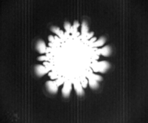
Figures 2(c) and 3 show the formation and collapse of the cavitation bubble with the viscous fingering interface structure as well as the Newton rings.
Evolution of cavitation bubble during surface separation. The wavelength of the unstable gas–liquid interface increases with  $h$ and decreasing speed of the interface. The black dots inside the bubble at later times are water droplets. Note that the contrast is adjusted separately for each picture to better display the cavitation event, and as a consequence, the Newton rings are not apparent.

3. Theory
Classical nucleation theory for homogeneous nucleation yields nucleation rates that are much too small to explain nucleation at our pressure and time scales. Only at negative pressures two orders of magnitude larger than in our experiment do bubbles nucleate in the bulk (Menzl et al. Reference Menzl, Gonzalezc, Geigera, Caupind, Abascale, Valerianie and Dellagoa2016). This leaves heterogeneous nucleation that may be caused by geometric or chemical impurities as the only viable explanation for our observed phenomenon. The different ramp speeds, which vary by a factor 36, will cause a corresponding range of  $\dot {h}$ values. The value of
 $\dot {h}$ determines the height
 $h_c$ at which cavitation happens as well as the size of the bubbles. Since the presence of impurities as well as the random thermal fluctuations may vary between experiments, so will the onset of cavitation at a given
 $\dot {h}$.
The theory deals with the evolution after nucleation has taken place, and aims to reveal the hydrodynamics of the subsequent process. It will be on the assumptions of either constant or measured values of  $\dot {h}$.
3.1. Evolution of a circular bubble
To establish a theoretical understanding of the bubble evolution, we will also assume a circular bubble, an assumption that may be partly justified by the a posteriori observation that the amplitude of the branching structures is significantly smaller than the scale over which the pressure field varies. Before the bubble is formed, mass conservation of the liquid implies that the added volume under the ball as it is rising must be balanced by a corresponding influx. We may write the volume change within a radius  $r$ as
 \begin{equation} \dot{V} (r)= {\rm \pi}r^2 \dot{h} = 2{\rm \pi} r (h+\Delta h )\,u(r). \end{equation}
The increase in separation  $\Delta h = r^2/(2R)$ follows from the geometric observation that the angle
 $\alpha$ in figure 1(b) occurs in several places. This implies that the gap-averaged fluid velocity takes the form
 \begin{equation} u(r) ={-}\frac{\dot{h} r/2}{h + r^2/(2R)} . \end{equation}
This velocity decays to 0 at  $r=0$ for symmetry reasons, and has a maximum at
 $r=\sqrt {2hR}$. Using the corresponding maximum velocity
 $u_m= \dot {h}\sqrt {R/(8h)}$ and separation
 $h= 1\ \mathrm {\mu } {\rm m}$ (see figure 2b), we may compute the upper bound of the Reynolds number
 $Re=u_mh/\nu <0.5$, where
 $\nu$ is the kinematic viscosity of water, and
 $\dot {h}$ and
 $h$ are estimated from figure 2(b).
Since  $Re$ is small, we may take the Stokes equation to govern the fluid pressure
 $P(r)$. Moreover, since the radius of curvature of the streamlines
 ${\sim }R$ is much larger than the gap, we may apply a lubrication limit of this equation. This equation will rely on the velocity field of (3.2), and may be written as
 \begin{equation} \frac{\partial P}{\partial r} = 6\mu \dot{h}\,\frac{r}{(h+r^2/(2R))^3}, \end{equation}
where  $\mu$ is the dynamic viscosity. Integrating this from
 $r$ to
 $\infty$, where the fluid has the atmospheric background pressure
 $P_0$, yields
 \begin{equation} P(r) = P_0 - \frac{3\mu R \dot{h}}{h^2(1 +r^2/(2Rh))^2} \end{equation}
for the pressure field that exists before the bubble is formed.
Once a bubble of radius  $r_c(t)$ is formed, the conservation of liquid volume inside a radius
 $r$ may be described as
 \begin{equation} \dot{V} (r) = {\rm \pi}(r^2-r_c^2) \dot{h} = 2{\rm \pi} r_c (h+ \Delta h(r_c) ) \dot{r}_c - 2{\rm \pi} r (h+ \Delta h (r)) u, \end{equation}
where we have neglected the mass loss due to the vapour that is formed inside the bubble. This gives the velocity
 \begin{equation} u(r) = \frac{h+r_c^2/(2R)}{h+r^2/(2R)}\,\frac{r_c}{r}\,\dot{r}_c - \frac{(r^2 -r_c^2 )\dot{h}/(2r)}{h+r^2/(2R)} . \end{equation}
With this velocity field the lubrication approximation of the Stokes equation becomes
 \begin{equation} \frac{\partial P}{\partial r}= \frac{6\mu \left( (r^2-r_c^2)\dot{h} - 2r_c \dot{r}_c (h+r_c^2/(2R)) \right) }{(h + r^2/(2R))^3r} . \end{equation}
Since the vapour pressure at room temperature is  ${\sim }0.03\ \mathrm {atm}$, which will turn out to be three orders of magnitude smaller than the typical liquid pressures, we take it to be zero and integrate (3.7) from
 $r=r_c$, where
 $P=0$, to
 $r= \infty$, where
 $P=P_0$.
Following ch. 11.2 in Israelachvili (Reference Israelachvili2011), the order of magnitude of the van der Waals forces between a sphere of radius  $R$ and a surface may be estimated as
 ${\sim }1\ \mathrm {\mu } \text {N}$ if the separation is taken as
 $h=10$ nm. The vertical force on the plate due to surface tension is
 $2{\rm \pi} r_c \sim 4\ \mathrm {\mu } \text {N}$ if
 $r_c=10\ \mathrm {\mu } \text {m}$. On the other hand, the local forces due to the negative water pressures
 $P \sim -10\ \mathrm {atm}$ is
 $F_P\approx {\rm \pi}r_c^2 P \sim 100\ \mathrm {\mu } \text {N}$, so that the hydrodynamic force dominates the van der Waals and capillary forces by two orders of magnitude as the bubble is first recorded.
However, the capillary pressure drop  $P_c$ across the water vapour interface – which is due to the surface tension and the curvature in the vertical direction, and depends on the dynamic wetting angle
 $\alpha _w \approx 50^\circ$ of the water – is not negligible at the very start of the bubble growth. The pressure
 $P_c = 2 \sigma \cos \alpha _w/h \approx 15\ \mathrm {atm}$ when
 $h=40\ \mathrm {nm}$, corresponding to frame (2) of figure 2(c), quickly drops to
 $P_c \approx$1 atm somewhere between the
 $h$ values of frames (2) and (3) of figure 2(c). For simplicity, we will neglect
 $P_c$ in the calculation of the
 $r_c(t)$ evolution. As we will see, this limits the model to describe the later part of the bubble evolution (shown in frames (2)–(4) of figure 2c) when the capillary pressure becomes small compared to the viscous pressure drop.
Integration then gives
 \begin{equation} \frac{P_0R}{6\mu \dot{h}} = K(r_c) - I(r_c)\left( \frac{r_c^2}{R^2} + \frac{2r_c \dot{r}_c h}{R^2\dot{h}} \left( 1 + \frac{1}{x_c} \right)\right), \end{equation}
where we have introduced the integrals
 \begin{equation} \left.\begin{gathered} I(r_c)=R^3\int_{r_c}^{\infty} \frac{{\rm d}r}{r(h+r^2/(2R))^3} = \frac{1}{2}\left( \frac{R}{h} \right)^3 g(x_c),\\ K(r_c) = R \int_{r_c}^{\infty} \frac{{\rm d}r\,r}{(h+r^2/(2R))^3} = 2\left( \frac{R}{r_c} \right)^4 \frac{1}{(x_c+1)^2}, \end{gathered}\right\} \end{equation}
where  $x_c=2Rh/r_c^2= 2{\rm \pi} Rh/A$,
 $A(t)={\rm \pi} \,r_c^2(t)$, and we have introduced the function
 \begin{equation} g(x_c) = \ln (x_c+1) - x_c\,\frac{1+3x_c/2}{(x_c+1)^2}. \end{equation}
An equation similar to (3.8) has been derived for the lubrication flow between parallel plates by Tirumkudulu & Russel (Reference Tirumkudulu and Russel2003). Now, solving (3.8) for  $\dot {r}_c$ brings it to the form
 $\dot {r}_c = F(h,\dot {h},r_c)$, which allows us to solve the numerical scheme
 \begin{equation} r_c \rightarrow r_c + F(h,\dot{h}, r_c) \,{\rm d}t, \end{equation}
where  $h=h(t)$ and
 $\dot {h} = \dot {h} (t)$ are the measured values. The result of such a calculation for a single experiment is shown in figure 4(a), while figure 4(b) shows the early-time result for all experiments.
(a) The bubble radius as a function of time when  $h(t)$ and
 $\dot {h}$ are taken as the measured values from a typical experiment (dots) along with the calculation based on (3.11) (line). Cavitation time
 $t_c$ is estimated as the lowest root of a parabolic fit of the data. (b) Comparison between the measured and calculated values of the first recorded bubble radii from all the experiments; the first value is shown by blue dots, and the second by green triangles. The red line has slope 1.

3.2. Pressure field
With the values of  $r_c(t)$ at hand, (3.7) may be used to calculate the pressure field
 $P(r)$ for
 $r>r_c$. Integrating this equation from
 $r$ to
 $\infty$ gives
 \begin{equation} P(r) = P_0 - 6\mu \left( \left(K(r)-I(r)\,\frac{r_c^2}{R^2}\right) \frac{\dot{h}}{R} - \frac{2r_c \dot{r}_c h}{R^3}\,I(r) \left( 1+\frac{1}{x_c}\right) \right), \end{equation}
where the argument  $r$ in
 $I$ and
 $K$ means that
 $x= 2Rh/r^2$ must be used in place of
 $x_c$ in (3.9).
3.3. Scaling behaviour from constant  $\dot {h}$ theory

The rather weak agreement between theory and measurement that is displayed in figure 4(a) is greatly improved by the introduction of non-dimensional variables and the consideration of their scaling behaviour.
The extension of a piezoelectric element has a linear relationship with the applied voltage, and in the experiments, this voltage is increased linearly with time during the initial ramp. Therefore, the height  $h$ would increase linearly in time as well, save for the effects of elastic deformations of the support system. Such an elastic response is clearly present, as is evident from the oscillations in
 $h(t)$, shown in figure 2(a). However, figure 2(b) shows that during the existence of the bubble, a linear increase of
 $h(t)$ may be a reasonable approximation, which we will apply in the following. This is also justified by the possibility of constructing future, more rigid experimental set-ups.
Introducing the characteristic time scale
 \begin{equation} \Delta t = \sqrt{\frac{12\mu R}{P_0 \dot{h}}} \end{equation}
and area
 \begin{equation} A_0 = \frac{24 \mu}{P_0\,\Delta t}\,{\rm \pi} R^2 , \end{equation}
we may rewrite (3.8) in terms of the dimensionless variables  $t'=t/\Delta t$ and
 $A'=A/A_0$. The point of doing this is (i) to establish a dynamic equation with relevant dimensionless groups, (ii) to obtain the scaling behaviour relating the control parameters to the bubble area and lifetime, and (iii) to identify the limits to this scaling behaviour.
By assumption,  $h(t)=\dot {h} t$, so the theoretical time of cavitation is
 \begin{equation} t_c = \frac{h_c}{\dot{h}}. \end{equation}
In terms of the dimensionless variables, the different terms of (3.8) then take the form
 \begin{equation} \left.\begin{gathered} \frac{P_0R}{6\mu \dot{h}}= 8 \left(\frac{{\rm \pi} R^2}{A_0} \right)^2,\\ \frac{2r_c \dot{r}_c h}{R^2\dot{h}}=\frac{A_0}{{\rm \pi} R^2}\,t'\,\frac{{\rm d}A'}{{\rm d}t'},\\ \frac{r_c^2}{R^2}= \frac{A_0}{{\rm \pi} R^2}\,A',\\ x_c= \frac{ t'}{A'},\\ K(x_c,A') = 2 \left(\frac{{\rm \pi} R^2}{A_0} \right)^2\frac{1}{A'^2(x_c+1)^2},\\ I(x_c) = 4 \left(\frac{{\rm \pi} R^2}{A_0} \right)^3 \frac{g(x_c)}{t'^3}. \end{gathered}\right\} \end{equation}
Combining the above results, (3.8) may be written as
 \begin{equation} \frac{{\rm d}A'}{{\rm d}t'} = \frac{t'}{t'+A'} \left( \frac{t'^2}{g(x_c)} \left( \frac{1}{2(t'+A')^2} - 2\right) - \frac{A'}{t'}\right) , \end{equation}
where all dimensional quantities, such as  $P_0$,
 $R$ and
 $\mu$, have dropped out.
This equation may be solved numerically subject only to the initial condition  $A'(t'_c) = A'_c$. The dependence on
 $A'_c$ may be neglected as long as
 $A_c \sim h_c^2$; replacing
 $A_c$ by its
 $A_c\rightarrow 0$ limit changes the subsequent
 $A(t)$ values by less than 1 %.
The non-dimensionalized initial times  $t'_c =h_c/(\dot {h}\,\Delta t)$, which are obtained from the experiments, are shown in figure 5(b). Using the extreme values of this figure,
 $t'_c = 0.035$ and 0.15 (neglecting only the single
 $t'_c=0.25$ point), we obtain the non-dimensionalized areas
 $A'(t')$ shown by the red and green curves in figure 6. For the smaller
 $t'_c$ values, when
 $t_c' \le 0.001$,
 $A'$ has essentially converged to its
 $t'_c \rightarrow 0$ limit.
(a) The pulling velocity  $\dot {h} = \textrm {d}h/\textrm {d}t$ at the point of cavitation, along with the corresponding height
 $h$. The blue dots show the initial
 $h$ measurements, and the green dots show the values at the time immediately before the bubble is observed. The black dots show the values immediately after cavitation, and the red line is a linear fit to the latter data to guide the eye. (b) The effective non-dimensionalized initial time
 $t'_c =h_c/(\dot {h}\,\Delta t)$ as a function of
 $h_c$.

Normalized bubble area versus normalized time for the extreme  $t'_c$ values shown in figure 5(b), as well as the values
 $t'_c=0.01{-}0.0001$.

Figure 6 shows that  $A'(t')$ varies significantly with
 $t'_c$ over the experimental range
 $t'_c=0.035{-}0.15$, and when
 $t'_c$ becomes larger than these values, the bubble will simply not grow. However, when the area (see figure 7) is normalized by its maximum value
 $A_m$, rather than
 $A_0$, and the time is normalized by the bubble lifetime
 $t_l$, rather than
 $\Delta t$, the dependence on
 $t'_c$ becomes much smaller. This is illustrated in figure 8(a) where the predicted variation of
 $A(t)/A_m$ with
 $t'_c$ is less than 5 % over the full experimental range. This variation is smaller than the experimental uncertainty, so the prediction is that the area may be written in the form
 \begin{equation} \frac{A(t)}{A_m} = f\left(\frac{t-t_c}{t_l}\right) \end{equation}
for a curve  $f(x)$, which is the same for all the cavitation bubbles within the experimental uncertainty. The predicted data collapse of
 $A(t)/A_m$ is shown in figure 8(a), using the experimental data of figure 7.
Bubble area versus the post nucleation time  $t_c$. A parabolic fit to each of the data series from the 37 experiments yielded bubble nucleation times, maximum areas, and bubble lifetimes
 $t_l$. All the data were then rescaled to give the plot in figure 8(a).

(a) Collapse of normalized bubble area versus normalized bubble lifetime for experimental data (dots) and theory (lines). The theory is shown for both the smallest and largest measured values of  $t'_c =h_c/(\dot {h}\,\Delta t)$. (b) Maximum bubble area versus bubble lifetime from experimental data (dots), a linear fit to data of slope
 $-1.0$ (solid black line), the theory given by (3.19) (solid red line), and the theory using the asymptotic value
 $A'_m=0.0698$ (dashed black line). Note that the experimental areas and lifetimes have been computed by the maximum value and the difference of the roots of a quadratic fit of the experimental data.

The normalized bubble lifetime value  $t'_l=0.770$ is obtained by inspection of the
 $t'_c<0.01$ graphs in figure 6. However, when
 $t'_c \gtrsim 0.01$,
 $t'_l$ and the maximum value
 $A'_m$ will depend on
 $t'_c$. The corresponding maximum area is
 \begin{equation} A_m = A_0\,A'_m(t'_c) = A'_m (t'_c)\,\frac{ 24 \mu {\rm \pi}R^2}{ P_0 }\,\frac{1}{\Delta t}, \end{equation}
where the replacement  $\Delta t = t_l/t'_l$ gives
 \begin{equation} A_m = A'_m (t'_c)\,t'_l(t'_c)\,\frac{ 24 \mu {\rm \pi}R^2}{ P_0 }\,\frac{1}{ t_l} . \end{equation}
In the limit when  $t'_c \ll 0.01$, we may replace
 $A'_m (t'_c)\,t'_l(t'_c) \rightarrow 0.0524$, and we are left with the asymptotic scaling
 $A_m \propto 1/t_l$.
On the other hand, we may also use (3.13) to express  $A_m$ by
 $\dot {h}$ and
 $R$. This yields
 \begin{equation} A_m = 4A'_m{\rm \pi}\,\sqrt{\frac{3\mu \dot{h}}{P_0}}\,R^{3/2}, \end{equation}
which shows how the maximum bubble area depends on the radius of curvature of the lens. This is of some significance relative to the ‘lifted Hele-Shaw cell’ experiments for which  $R\rightarrow \infty$. In this case, the prediction is that the bubble would always extend beyond the finite boundaries of the cell.
Figure 8(b) shows to what extent the predicted  $A_m\propto 1/t_l$ scaling is fulfilled in the experiment. The theoretical prediction, which is shown in figure 8(b) (red line), is given by (3.19), which is obtained by setting
 $h_c=30$ nm and varying
 $\dot {h}$ to get a range of values for
 $\Delta t$ and
 $t'_c$ as given by (3.13) and (3.14), respectively. The corresponding asymptotic
 $t'_c\rightarrow 0$ result, which is shown by the dashed line, is given by (3.20). The solid black line which is a linear fit to the experimental data of slope
 $-1.0$, seems to indicate agreement with the asymptotic result. However, the uncertainty in the
 $t_l\gtrsim 1$ ms data may also yield agreement with the non-asymptotic theory (red line). The uncertainty is caused mainly by the fact that the experimental lifetimes are extracted from the curves of figure 7 by fitting these curves to parabolas and defining the lifetimes as the distance between their roots. This procedure may cause errors, in particular for longer lifetimes. However, for the
 $t'_c$ values where
 $A'_m$ and
 $t'_l$ have converged, i.e. when
 $t_l\lesssim 1$ ms, the predicted asymptotic scaling behaviour of
 $A_m$ is well satisfied by the experiments.
3.4. Pressure field and secondary nucleation
Figure 9 shows the pressure in the water outside the growing bubble at subsequent times. It is calculated from (3.12), using the measured values of  $\dot {h}$ and the corresponding calculated values of
 $\dot {r}_c$. During the early expansion phase, figure 9 shows how the pressure outside the bubble occasionally falls below the initial cavitation pressure given by (3.4), and sometimes not. This variability in the water tension, and the fact that defects or impurities away from the centre may cause nucleation at pressures less negative than that required at the centre, may explain the occasional secondary nucleation events. However, the radius at which this outside pressure reaches its minimum is approximately
 $r_c \sim 20\ \mathrm {\mu } \textrm {m}$, a size that is reached within
 $\sim$0.05 ms. On the other hand, figure 2(b) shows that the largest initial
 $\dot {h}$ values exist for a time
 $\sim$0.5 ms. Hence the time available for secondary nucleation is an order of magnitude smaller than the time available for the primary nucleation, an observation that agrees well with the fact that only occasionally is such a secondary bubble observed in the experiments, as is illustrated in figure 9.
(a,b) The water pressure outside the expanding bubble as a function of  $r>r_c$ for the two different measured time series
 $h(t)$. Red curve: earliest
 $r_c$ value. Dashed curves: when the bubble has reached
 $r_c= 2.5\ \mathrm {\mu } \textrm {m}$,
 $5\ \mathrm {\mu } \textrm {m}$,
 $7.5\ \mathrm {\mu } \textrm {m}$, …, and
 $\dot {r}_c >0$. The blue dots represent the pressure given by (3.4) with
 $r=0$ at the time when the cavitation bubble is formed. (c) Image of a cavitation bubble with a secondary bubble nucleated outside the main bubble. Scale bar is
 $20\ \mathrm {\mu } \textrm {m}$.

3.5. Saffman–Taylor instability
As the bubble grows, a less viscous fluid (the water vapour) displaces the more viscous water, creating the conditions for the Saffman–Taylor instability to develop. Linear stability analysis (Feder, Flekkøy & Hansen Reference Feder, Flekkøy and Hansen2022) predicts that the fastest-growing perturbation has wavelength
 \begin{equation} \lambda_m = {\rm \pi}(h+ \Delta h) \sqrt{\frac{\sigma}{\mu \dot{r}_c}} , \end{equation}
where  $h+\Delta h$ is the local gap width at
 $r=r_c$. Figure 10 shows
 $\lambda _m$ as a function of
 $h$ for all the experiments, using the
 $\dot {r}_c$ values obtained from (3.11) along with the measured
 $h$ values, and viscosity
 $\mu =10^{-3}\ \mathrm {Pa}\ \mathrm {s}$. Since the time step used in that calculation is smaller than the time between the frames at which
 $h$ is measured, the calculated
 $\dot {r}_c$ value that enters in (3.22) evolves numerically between each recorded
 $h$ value. This is why there are several
 $\lambda _m$ values for each
 $h$ value, effectively providing a measure of uncertainty in the predicted
 $\lambda _m$ values. The red dots, which are obtained by estimating the finger number from figure 3, fall below the approximately linear trend shown by the grey dots. The sign of this discrepancy is the same as that found by Lindner et al. (Reference Lindner, Derks and Shelley2005).
The dominant Saffman–Taylor wavelength as a function of  $h$. The blue and grey dots show the
 $\lambda _m$ values given by (3.22) using the
 $\dot {r}_c$ values computed from (3.11) and all the experimental
 $h$ values, with the blue dots corresponding to the experiment shown in figure 3. The red dots show the actual wavelength that is determined by counting the fingers in figure 3.

However, initially at small  $h$ values, there is an approximate agreement between the measured and predicted
 $\lambda _m$ values, which strongly suggests that the finger structure is indeed caused by the Saffman–Taylor instability. At later times, the smaller
 $\lambda _m$ fingers will already have grown to a point where they will dominate the larger
 $\lambda _m$ perturbations, which come to have the larger growth rates too late to dominate the earlier growth.
4. Discussion and conclusion
Figure 4(a) shows the result of applying the numerical scheme of (3.11) starting from a small bubble with  $r_c(0)=h_0$, the initial separation, and integrating (3.8). The values of
 $r_c$ are calculated using the measured values of
 $h(t)$ and
 $\dot {h} (t)$, not a constant
 $\dot {h}$, at this point. Figure 4(a) also shows a comparison between the circular bubble calculations and a single experimental time series for the
 $r_c(t)$ values. The discrepancy that is seen between the calculated and measured values is most likely caused by the development of branching structures that start immediately after the bubble cavitates, while the theory assumes a circular bubble. Except for the last value, the experimental
 $r_c$ values fall under the theoretical prediction. This is to be expected as the formation of vapour fingers will tend to reduce the pressure gradients in the liquid left between them. This pressure screening is a well-known effect in viscous fingering structures that grow radially in a porous medium or Hele-Shaw cell, as noted by Måløy, Feder & Jøssang (Reference Måløy, Feder and Jøssang1985). As a result, only part of the liquid surrounding the growing bubble is subject to a significant outward driving force. By contrast, around a circular bubble, the pressure gradient is everywhere in the radial direction, and is at its largest at the interface.
In figure 7, the projected area  $A(t)$ of the growing and collapsing bubble is shown. While the lifetime
 $t_l$ varies by factor 10, the rise velocity
 $\dot {h}$ varies by a factor
 $\sim$36, which is the variation of the ramp speed. Hence the data collapse, and
 $A_m \propto 1/ t_l$ scaling seen in figure 8 is supported by a relatively wide range of experimental conditions.
Assuming the cavitation bubble to have a circular shape resulting from a constant pulling speed is clearly not realistic. However, the length scale  $\sqrt {2Rh}$ over which the pressure decays theoretically (see figure 9) is significantly larger than the bubble radius, indicating that the large-scale pressure gradients are insensitive to the local interface perturbations. Since these long-range gradients are the driving force behind the bubble collapse, it is not surprising that general features, such as the exponent governing the Family–Vicsek scaling (Vicsek & Family Reference Vicsek and Family1984), which is predicted in (3.18), survive the model simplifications.
Figure 5(a) shows a certain correlation between the pulling velocity  $\dot {h}$ at the point of cavitation and the corresponding height
 $h_c$. It displays a variation of
 $\dot {h}$ by factor 30. The initial time
 $t'_c$ that is shown in figure 5(b), on the other hand, displays a variation by less than factor 2 around its mean value
 ${\lesssim }0.1t_l$. This means that the description provided by the non-dimensionalized equation (3.17), along with the initial condition at
 $t_c$, is close to common for all the experiments despite the great variability in the pulling speed
 $\dot {h}$.
Figures 8(a) and 8(b) are based on the determination of  $A_m$ from the fluctuating experimental data. The measured
 $A(t)$ curve was fitted to a parabola, and the value of
 $A_m$ was taken as the maximum of this parabola, and the nucleation and collapse times were identified as its zero points. The non-parabolic component in the data causes the parabolic fit to underestimate the maximum by 5 %–10 %, hence the maximum value in the
 $A(t)/A_m$ curve overshoots 1 correspondingly.
The scaling behaviour that is predicted by (3.20) amounts to stating that the larger the bubble, the shorter it lives. This counter-intuitive result is seen to describe both the idealized circular bubbles and the experimental ones: figure 8(b) shows the predicted and measured maximum area that is reached by the bubbles, as a function of  $t_l$; the experimental data are well fitted by a straight line of slope
 $-1$. However, the theory predicts a maximum area of about three times the measured values. This discrepancy is likely caused by the fingering at the interface, the fact that
 $\dot {h}$ is not constant but increases right after cavitation, and the neglect of capillary forces in the theory. Given the upward moving boundary, there is no reason for the flow around the bubble to be reversible. It is therefore to be expected that the branched interface takes longer to collapse back into a point than the circular one. On the other hand, the effect of the neglected capillary pressure would be to accelerate the process and reduce the bubble lifetime. Qualitatively, the unknown contribution from the capillary forces could be included in the theory by an increase in the driving pressure
 $P_0$ in (3.13), from which it is clear that the bubble lifetime decreases as
 $P_0$ increases.
The fact that  $A_m$ increases with decreasing lifetime is perhaps most easily understood physically, or intuitively, by noting that
 $\dot {h}$ sets the speed of the entire process, and that when
 $\dot {h}$ becomes sufficiently small, cavitation will not happen at all. When the whole process is fast, it is reasonable that the bubble lifetime is short, and only above some critical
 $\dot {h}$ will
 $A_m$ be finite, starting at some small value. As
 $\dot {h}$ increases, so will
 $A_m$, and as a combined result, there is an inverse relationship between
 $A_m$ and
 $t_l$, which by analysis turns out to be governed by an exponent
 $-1$. The
 $A_m \propto 1/ t_l$ scaling behaviour is in strong contrast to that observed for inertia-dominated cavitation bubbles, such as those observed around propellers, where the lifetime scales as
 $t_l \propto R_{max}$, the maximum bubble radius; see ch. 15 in Kim et al. (Reference Kim, Franc and Karimi2014).
In summary, we have established an experimental technique that resolves the boundary separation between a sphere and a flat surface on the nanometre scale and allows the detailed observation of  ${\sim }10\ \mathrm {\mu }\textrm {m}$ size cavitation bubbles formed by creeping flow hydrodynamics. Contrary to the much-studied cavitation processes governed by inertia, these bubbles exhibit a scaling behaviour where their lifetime is inversely proportional to their maximum size. Although the interface develops Saffman–Taylor fingers and a branched structure, this scaling exponent is captured by a theory relying on the assumption that bubbles are circular.
Supplementary movies
Supplementary movies are available at https://doi.org/10.1017/jfm.2024.937.
Funding
This work was partly supported by the Research Council of Norway through its Centers of Excellence funding scheme, project no. 262644. T.C. was supported by the UiO:LifeScience grant Abino.
Declaration of interests
The authors report no conflict of interest.


 Open access

