1 Introduction
The instability of the flow between two differentially rotating cylinders with the fluid being stably stratified is an idealized setting which may be of relevance to processes in the atmosphere and oceans (Hart Reference Hart1979; Plougonven & Zhang Reference Plougonven and Zhang2014) and accretion disks (Avila Reference Avila2012). For the most part, stratified Taylor–Couette flow has been considered in regimes where the annular gap between the two cylinders is relatively small, and theoretical treatments usually assume periodicity in the axial direction. Molemaker, McWilliams & Yavneh (Reference Molemaker, McWilliams and Yavneh2001) and Yavneh, McWilliams & Molemaker (Reference Yavneh, McWilliams and Molemaker2001) showed that, even when the hydrodynamics is centrifugally stable, stable stratification can lead to instability due to a resonant interaction between non-axisymmetric inertia–gravity waves trapped near each of the two cylinders. This instability has come to be known as the strato-rotational instability (SRI), and it was first observed experimentally by Le Bars & Le Gal (Reference Le Bars and Le Gal2007).
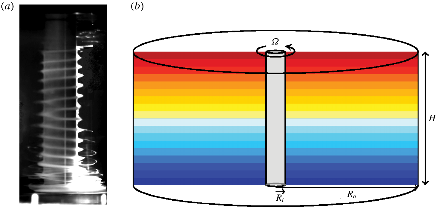
(a) Dye visualization of two helical waves travelling along the rotating inner cylinder from the top and bottom, reproduced from Flór et al. (Reference Flór, Hirschberg, Oostenrijk and van Heijst2018). The flow conditions correspond to salt-stratified Taylor–Couette flow in the very wide gap regime with radius ratio  $\unicode[STIX]{x1D702}=R_{i}/R_{o}=1/15$, Froude number
 $Fr=0.53$ and inner cylinder Reynolds number
 $Re_{i}=521$. The dimensions of their annulus are inner radius
 $R_{i}=2.5~\text{cm}$, outer radius
 $R_{o}=37.5~\text{cm}$ and working depth
 $H=40~\text{cm}$. (b) Schematic of the fluid domain, including the initial temperature stratification
 $T_{in}(z)$.

Our present investigation is motivated by the recent experiments of Flór et al. (Reference Flór, Hirschberg, Oostenrijk and van Heijst2018) who found spiral structures confined to the inner rotating cylinder in a regime where the ratio of the inner to outer cylinder radii is quite small,  $R_{i}/R_{o}=1/15$; see figure 1(a) for a visualization of the flow from their experiments. This is a very different regime to that typically studied for SRI. The spiral structures they observed are reminiscent of the radiative instability (RI) reported by Riedinger, Le Dizès & Meunier (Reference Riedinger, Le Dizès and Meunier2011), who considered a rotating cylinder in a large rectangular tank of stratified fluid. Using a large axial wavenumber approximation, Le Dizès & Riedinger (Reference Le Dizès and Riedinger2010) showed how RI and SRI are related, with SRI being transformed into RI as the gap between the two cylinders becomes large. As well as conducting experiments, Riedinger et al. (Reference Riedinger, Le Dizès and Meunier2011) considered the linear stability analysis of the potential flow around an isolated rotating cylinder of infinite axial length in a linearly stratified medium (i.e. the velocity of their base flow had azimuthal component
 $v\propto 1/r$, zero meridional components
 $u=w=0$ and extended radially out to
 $r\rightarrow \infty$). They mostly considered inviscid flow, and presented some comments on viscous effects. The main mode of instability was found to result in helical waves with azimuthal wavenumbers that depend on the Froude number
 $Fr=\unicode[STIX]{x1D6FA}/N$ and a Reynolds number
 $Re_{i}=\unicode[STIX]{x1D6FA}R_{i}^{2}/\unicode[STIX]{x1D708}$, where
 $N$ is the Brunt–Väisälä buoyancy frequency,
 $\unicode[STIX]{x1D6FA}$ the rotation rate of the cylinder of radius
 $R_{i}$ and
 $\unicode[STIX]{x1D708}$ is the kinematic viscosity. Their experiments were conducted in a salt-stratified tank of horizontal cross-section
 $240~\text{cm}\times 74~\text{cm}$ and depth 48 cm, which was filled to a height of 45 cm. Their experiments used three different cylinders of radii
 $R_{i}=12.5$, 15 and 20 cm. They typically observed instabilities consisting of helical waves travelling up (down) from the bottom (top). They expected the flow to have up–down reflection symmetry, but noted: ‘nevertheless, in a few cases, we observe that one of the two waves can be dominant’, and ‘there is a difference between the frequencies of the two waves … slow drift toward the top’. They also noted that the stratification
 $N$ was not uniform across the depth, with departures in the top and bottom 10 cm of the depth, which they ascribed to salt diffusivity, turbulent mixing and evaporation effects. They did not consider centrifugal buoyancy effects as a potential contributor.
For the most part, centrifugal buoyancy effects in stratified Taylor–Couette flows have been ignored. Barcilon & Pedlosky (Reference Barcilon and Pedlosky1967) suggested that centrifugal buoyancy effects may not be negligible, and Shalybkov & Rüdiger (Reference Shalybkov and Rüdiger2005) raised the cautionary point that the use of the usual Boussinesq approximation (which does not account for centrifugal buoyancy) for small Froude numbers seems to still be an open question. Rüdiger et al. (Reference Rüdiger, Seelig, Schultz, Gellert, Egbers and Harlander2017) considered the centrifugal buoyancy for parameter regimes corresponding to their experiments, and concluded that since  $R_{i}\unicode[STIX]{x1D6FA}^{2}/g$ is small (where
 $g$ is gravitational acceleration), that they could neglect centrifugal buoyancy effects. They also studied the linear stability of stratified Taylor–Couette flow assuming a unidirectional base flow and periodicity in the axial direction, and found discrepancies between model and experimental results which they suggested may stem from the model ignoring endwall effects, but exploring these was ‘beyond the scope’ of their study.
So far, the theoretical studies of stratified Taylor–Couette flow (e.g. Hua, Le Gentil & Orlandi Reference Hua, Le Gentil and Orlandi1997; Shalybkov & Rüdiger Reference Shalybkov and Rüdiger2005; Gellert & Rüdiger Reference Gellert and Rüdiger2009; Park & Billant Reference Park and Billant2013; Leclereq, Nguyen & Kerswell Reference Leclereq, Nguyen and Kerswell2016; Rüdiger et al. Reference Rüdiger, Seelig, Schultz, Gellert, Egbers and Harlander2017; Park et al. Reference Park, Billant, Baik and Seo2018) have considered the axial direction to be periodic and the base state to be the unidirectional flow of Taylor (Reference Taylor1923),
 $$\begin{eqnarray}v=Ar+B/r,\end{eqnarray}$$
where  $v$ is the azimuthal component of velocity and the constants
 $A$ and
 $B$ depend on the radii and rotation rates of the inner and outer cylinders, together with a linear vertical stratification. All physical experiments have finite axial length, and differential rotation between the bottom endwall and one or both cylinders (the top is sometimes open). This leads to vortex line bending near one or both corners where the rotating inner cylinder meets the stationary bottom and top endwalls, driving a secondary meridional flow. As such, the base flow is not unidirectional. This meridional flow will be shown here to be critical in determining the helical instability reported in the experiments of Flór et al. (Reference Flór, Hirschberg, Oostenrijk and van Heijst2018).
The outline of the paper is as follows. In § 2, the governing equations are described for the fully enclosed finite annulus with rotating inner cylinder, as is the numerical technique used to solve them. Section 2.1 describes the symmetries of the system, and how neglecting or accounting for centrifugal buoyancy affects them. Details of the basic state are given in § 3. These are contrasted with the idealized potential flow and circular Couette states. The influence of centrifugal buoyancy on the basic state is also described. Section 4 explores the primary instabilities when centrifugal buoyancy is ignored, showing that the extra symmetry that comes from ignoring centrifugal buoyancy results in peculiar dynamics. These peculiarities are removed in § 5 by accounting for centrifugal buoyancy, whose main impact is found to be that the helical wave instability occurs at the bottom corner (where the rotating cylinder meets the stationary bottom endwall) at a Reynolds number  $Re$ that is lower than the critical
 $Re$ when centrifugal buoyancy is ignored. For slightly larger
 $Re$, the top corner becomes unstable to another helical wave mode, and the two helical waves have slightly different frequencies leading to modulation dynamics. They have much in common with what is observed experimentally, and comparisons with those observations are presented in § 6.
2 Governing equations
Consider a completely fluid-filled annulus of height  $H$, inner radius
 $R_{i}$ and outer radius
 $R_{o}$. The outer cylinder, top and bottom walls are stationary and the inner cylinder rotates at constant angular velocity
 $\unicode[STIX]{x1D6FA}$. The top and the bottom walls are maintained at fixed temperatures,
 $T_{0}^{\ast }+\unicode[STIX]{x0394}T^{\ast }/2$ for the top endwall and
 $T_{0}^{\ast }-\unicode[STIX]{x0394}T^{\ast }/2$ for the bottom endwall, while both cylinders are insulated.
 $T_{0}^{\ast }$ is a reference temperature, and the temperature difference between the top and bottom
 $\unicode[STIX]{x0394}T^{\ast }$ is positive, so that the vertical temperature gradient is stabilizing. Gravity
 $g$ points downwards. The kinematic viscosity of the Newtonian fluid is
 $\unicode[STIX]{x1D708}$, its thermal diffusivity is
 $\unicode[STIX]{x1D705}$, and its coefficient of volume expansion is
 $\unicode[STIX]{x1D6FC}$. A schematic of the set-up is shown in figure 1(b).
Using the annular gap  $D=R_{o}-R_{i}$ as the length scale, the viscous diffusion time across the gap
 $D^{2}/\unicode[STIX]{x1D708}$ as the time scale,
 $\unicode[STIX]{x0394}T^{\ast }$ as the temperature scale and employing the Boussinesq approximation accounting for centrifugal buoyancy (Lopez, Marques & Avila Reference Lopez, Marques and Avila2013), the non-dimensional governing equations are
 $$\begin{eqnarray}\displaystyle & (\unicode[STIX]{x2202}_{t}+\boldsymbol{u}\boldsymbol{\cdot }\unicode[STIX]{x1D735})\boldsymbol{u}=-\unicode[STIX]{x1D735}p+\unicode[STIX]{x1D6FB}^{2}\boldsymbol{u}+Gr\,T\hat{\boldsymbol{z}}+\unicode[STIX]{x1D716}T(\boldsymbol{u}\boldsymbol{\cdot }\unicode[STIX]{x1D735})\boldsymbol{u}, & \displaystyle\end{eqnarray}$$
 $$\begin{eqnarray}\displaystyle & (\unicode[STIX]{x2202}_{t}+\boldsymbol{u}\boldsymbol{\cdot }\unicode[STIX]{x1D735})T=\unicode[STIX]{x1D70E}^{-1}\unicode[STIX]{x1D6FB}^{2}T,\quad \unicode[STIX]{x1D735}\boldsymbol{\cdot }\boldsymbol{u}=0, & \displaystyle\end{eqnarray}$$
where  $\boldsymbol{u}=(u,v,w)$ is the non-dimensional velocity field in the cylindrical polar coordinate system
 $(r,\unicode[STIX]{x1D703},z)$,
 $p$ is the dynamic pressure and
 $\hat{\boldsymbol{z}}$ is the unit vector in the vertical direction
 $z$. The term
 $\unicode[STIX]{x1D716}T(\boldsymbol{u}\boldsymbol{\cdot }\unicode[STIX]{x1D735})\boldsymbol{u}$ accounts for centrifugal buoyancy effects. The fluid domain is
 $r\in [r_{i},r_{o}]=[\unicode[STIX]{x1D702}/(1-\unicode[STIX]{x1D702}),1/(1-\unicode[STIX]{x1D702})]$,
 $\unicode[STIX]{x1D703}\in [0,2\unicode[STIX]{x03C0})$ and
 $z\in [-\unicode[STIX]{x1D6FE}/2,\unicode[STIX]{x1D6FE}/2]$, where
 $\unicode[STIX]{x1D702}=R_{i}/R_{o}$ is the radius ratio and
 $\unicode[STIX]{x1D6FE}=H/D$ is the aspect ratio. We shall fix the annular geometry to
 $\unicode[STIX]{x1D702}=0.07$ and
 $\unicode[STIX]{x1D6FE}=1$, very close to those of the experimental apparatus used in Flór et al. (Reference Flór, Hirschberg, Oostenrijk and van Heijst2018).
The boundary conditions for temperature and velocity are
 $$\begin{eqnarray}\displaystyle & r=r_{i}:\quad \unicode[STIX]{x2202}T/\unicode[STIX]{x2202}r=0,\quad u=w=0,~v=Re, & \displaystyle\end{eqnarray}$$
 $$\begin{eqnarray}\displaystyle & r=r_{o}:\quad \unicode[STIX]{x2202}T/\unicode[STIX]{x2202}r=0,\quad u=w=v=0, & \displaystyle\end{eqnarray}$$
 $$\begin{eqnarray}\displaystyle & z=-\unicode[STIX]{x1D6FE}/2:\quad T=-1/2,\quad u=w=0,~v=Re\,q(r), & \displaystyle\end{eqnarray}$$
 $$\begin{eqnarray}\displaystyle & z=\unicode[STIX]{x1D6FE}/2:\quad T=1/2,\quad u=w=0,~v=Re\,q(r), & \displaystyle\end{eqnarray}$$
 $$\begin{eqnarray}q(r)=\exp [-c(r-r_{i})],\quad \text{with }c=100.\end{eqnarray}$$
The radial function  $q(r)$ is almost zero everywhere except in a narrow interval (controlled by
 $c$) close to the rotating inner cylinder. In this way the boundary condition on
 $v$ is continuous, avoiding Gibbs phenomena associated with discontinuities in the numerical simulations, and mimics the gap that exists in any real device with the inner cylinder rotating and stationary endwalls. The value of
 $c$ is chosen such that
 $q$ decreases from 1 to 0.05 over 3 % of the annular gap.
The non-dimensional groups appearing in the governing equations and boundary conditions are
 $$\begin{eqnarray}\displaystyle & \text{Prandtl number}\quad \unicode[STIX]{x1D70E}=\unicode[STIX]{x1D708}/\unicode[STIX]{x1D705}, & \displaystyle\end{eqnarray}$$
 $$\begin{eqnarray}\displaystyle & \text{Reynolds number}\quad Re=\unicode[STIX]{x1D6FA}R_{i}D/\unicode[STIX]{x1D708}, & \displaystyle\end{eqnarray}$$
 $$\begin{eqnarray}\displaystyle & \text{Grashof number}\quad Gr=\unicode[STIX]{x1D6FC}g\unicode[STIX]{x0394}T^{\ast }D^{3}/\unicode[STIX]{x1D708}^{2}, & \displaystyle\end{eqnarray}$$
 $$\begin{eqnarray}\displaystyle & \text{relative density variation}\quad \unicode[STIX]{x1D716}=\unicode[STIX]{x1D6FC}\unicode[STIX]{x0394}T^{\ast }, & \displaystyle\end{eqnarray}$$
 $$\begin{eqnarray}\displaystyle & \text{radius ratio}\quad \unicode[STIX]{x1D702}=R_{i}/R_{o}, & \displaystyle\end{eqnarray}$$
 $$\begin{eqnarray}\displaystyle & \text{aspect ratio}\quad \unicode[STIX]{x1D6FE}=H/D, & \displaystyle\end{eqnarray}$$
 $D=R_{o}-R_{i}$. The Prandtl number is a ratio of fluid properties and is constant in a given experiment. The Grashof number
 $Gr$ and the relative density variation
 $\unicode[STIX]{x1D716}$ are proportional to the imposed temperature gradient, and their ratio is the Archimedes number
 $$\begin{eqnarray}Ar=Gr/\unicode[STIX]{x1D716}=gD^{3}/\unicode[STIX]{x1D708}^{2}.\end{eqnarray}$$
Since  $Ar$ is constant in any real experiment,
 $\unicode[STIX]{x1D716}=Gr/Ar$ is enslaved to
 $Gr$, and so there are only two independent dynamical parameters in the problem,
 $Re$ and
 $Gr$. Other non-dimensional numbers used in this and related studies are the ratio of buoyancy and rotation time scales, known as the Froude number
 $Fr=\unicode[STIX]{x1D6FA}/N$, where
 $N=\sqrt{\unicode[STIX]{x1D6FC}g\unicode[STIX]{x0394}T^{\ast }/H}$ is the Brunt–Väisälä frequency, and
 $R_{N}=ND^{2}/\unicode[STIX]{x1D708}$, the non-dimensional buoyancy frequency, which is the ratio of the viscous and buoyancy time scales. These are related to
 $Re$ and
 $Gr$
 $$\begin{eqnarray}Fr={\displaystyle \frac{Re}{R_{N}}}{\displaystyle \frac{D}{R}}_{i}={\displaystyle \frac{Re}{R_{N}}}{\displaystyle \frac{(1-\unicode[STIX]{x1D702})}{\unicode[STIX]{x1D702}}},\quad R_{N}=\sqrt{{\displaystyle \frac{Gr}{\unicode[STIX]{x1D6FE}}}}.\end{eqnarray}$$
The experiments of Flór et al. (Reference Flór, Hirschberg, Oostenrijk and van Heijst2018) used water with salt as the stratifying agent. Instead, we shall use temperature and fix the Prandtl number  $\unicode[STIX]{x1D70E}=6$, nominally corresponding to water at approximately
 $25\,^{\circ }\text{C}$. Flór et al. (Reference Flór, Hirschberg, Oostenrijk and van Heijst2018) used
 $Re_{i}=Re\,\unicode[STIX]{x1D702}/(1-\unicode[STIX]{x1D702})$ and
 $Fr$ to describe the parameter regimes of their experiments. With the non-dimensionalization we have used,
 $Re$ and
 $Gr$ are the non-dimensional groups that naturally appear. Note that neglecting centrifugal buoyancy corresponds to taking the limit
 $\unicode[STIX]{x1D716}\rightarrow 0$ in (2.1). The Archimedes number corresponding to the experiments of Flór et al. (Reference Flór, Hirschberg, Oostenrijk and van Heijst2018) is large,
 $Ar=6.272\times 10^{11}$, and so
 $\unicode[STIX]{x1D716}$ is small (less than 0.1), even for the largest
 $Gr$ used in the experiments. The helical instability that they reported, for example in their figure 3 (reproduced here in figure 1a), had
 $Fr=0.53$ and
 $Re_{i}=521$, corresponding to
 $Gr\approx 4.24\times 10^{10}$ and
 $Re=7294$. In the simulations we report on here, we fix
 $Gr=4\times 10^{10}$ and
 $\unicode[STIX]{x1D716}=0.064$, and consider variations in
 $Re$. Those results are also compared to simulations ignoring centrifugal buoyancy, obtained by setting
 $\unicode[STIX]{x1D716}=0$.
The governing equations are solved using a second-order time-splitting method with consistent boundary conditions for the pressure, as in Lopez & Marques (Reference Lopez and Marques2014). Spatial discretization is via a Galerkin–Fourier expansion in  $\unicode[STIX]{x1D703}$ and Chebyshev collocation in
 $r$ and
 $z$. The spatial and temporal resolution used was
 $n_{r}\times n_{z}\times n_{\unicode[STIX]{x1D703}}=150\times 300\times 26$ and
 $\unicode[STIX]{x1D6FF}t=4\times 10^{-7}$ for
 $Re<6300$ and
 $\unicode[STIX]{x1D6FF}t=2\times 10^{-7}$ for
 $Re\geqslant 6300$. All numerical simulations have been performed with a linear temperature stratification
 $T_{in}=z/\unicode[STIX]{x1D6FE}$ as the initial condition for temperature, or from the continuation of solutions obtained with this initial condition, in order to mimic the experimental set-up.
Other variables used in the present problem are the vorticity,  $\unicode[STIX]{x1D74E}=\unicode[STIX]{x1D735}\times \boldsymbol{u}=(\unicode[STIX]{x1D714}_{r},\unicode[STIX]{x1D714}_{\unicode[STIX]{x1D703}},\unicode[STIX]{x1D714}_{z})$, and the helicity density
 $He=\boldsymbol{u}\boldsymbol{\cdot }\unicode[STIX]{x1D74E}$. The kinetic energies of the azimuthal Fourier modes of the velocity field,
 $$\begin{eqnarray}E_{m}=\frac{1}{2}\int _{-\unicode[STIX]{x1D6FE}/2}^{\unicode[STIX]{x1D6FE}/2}\int _{r_{i}}^{r_{o}}\boldsymbol{u}_{m}\boldsymbol{\cdot }\boldsymbol{u}_{m}^{\ast }r\,\text{d}r\,\text{d}z,\end{eqnarray}$$
where  $\boldsymbol{u}_{m}$ is the
 $m$th Fourier mode of the velocity field and
 $\boldsymbol{u}_{m}^{\ast }$ is its complex conjugate, provide a convenient way to characterize the non-axisymmetric states.
2.1 Symmetries
The domain and boundary conditions have a symmetry group generated by arbitrary rotations  ${\mathcal{R}}_{\unicode[STIX]{x1D6FD}}$ around the annulus axis, and a reflection
 ${\mathcal{K}}$ about the mid-height plane. Their actions on the velocity and temperature are
 $$\begin{eqnarray}\displaystyle & {\mathcal{R}}_{\unicode[STIX]{x1D6FD}}:[u,v,w,T](r,\unicode[STIX]{x1D703},z,t)\mapsto [u,v,w,T](r,\unicode[STIX]{x1D703}-\unicode[STIX]{x1D6FD},z,t), & \displaystyle\end{eqnarray}$$
 $$\begin{eqnarray}\displaystyle & {\mathcal{K}}:[u,v,w,T](r,\unicode[STIX]{x1D703},z,t)\mapsto [u,v,-w,-T](r,\unicode[STIX]{x1D703},-z,t), & \displaystyle\end{eqnarray}$$
 $\unicode[STIX]{x1D6FD}$ is an arbitrary angle. The rotations
 ${\mathcal{R}}_{\unicode[STIX]{x1D6FD}}$ generate the group
 $SO(2)$, and the reflection
 ${\mathcal{K}}$ generates the group
 $Z_{2}$ since
 ${\mathcal{K}}^{2}$ is the identity;
 ${\mathcal{R}}_{\unicode[STIX]{x1D6FD}}$ and
 ${\mathcal{K}}$ commute (
 ${\mathcal{K}}{\mathcal{R}}_{\unicode[STIX]{x1D6FD}}={\mathcal{R}}_{\unicode[STIX]{x1D6FD}}{\mathcal{K}}$), and together they generate the group
 ${\mathcal{G}}=SO(2)\times Z_{2}$.
The temperature and incompressibility equations (2.2) are equivariant with respect to  ${\mathcal{G}}$. However, in the Navier–Stokes equations (2.1), the last term is not equivariant; it changes sign when reflected (applying
 ${\mathcal{K}}$). This centrifugal buoyancy term renders the full system to not be reflection symmetric. The denser fluid at the bottom endwall is centrifuged outwards, while the lighter fluid near the top endwall is centrifuged inwards, generating a large scale circulation that breaks
 ${\mathcal{K}}$. In summary, if
 $\unicode[STIX]{x1D716}=0$ then
 ${\mathcal{G}}$ is the symmetry group of the problem, but when
 $\unicode[STIX]{x1D716}\neq 0$ the symmetry group is only
 $SO(2)$.
3 Basic states
In the limit of the annulus height-to-gap aspect ratio  $\unicode[STIX]{x1D6FE}\rightarrow \infty$, and ignoring centrifugal buoyancy (setting
 $\unicode[STIX]{x1D716}=0$), the basic state is described by the unidirectional circular Couette flow (1.1). For a stationary outer cylinder this unidirectional basic state has azimuthal velocity
 $$\begin{eqnarray}v(r)=Re\frac{\unicode[STIX]{x1D702}}{1-\unicode[STIX]{x1D702}^{2}}\left(\frac{r_{o}}{r}-\frac{r}{r_{o}}\right).\end{eqnarray}$$
The  $-r/r_{o}$ contribution is due to the presence of the stationary outer cylinder. If the outer cylinder were not there, i.e. taking the limit
 $r_{o}\rightarrow \infty$, the basic state would be a potential flow with
 $v(r)=r_{i}Re/r$. The
 $-r/r_{o}$ contribution is largest at the outer cylinder, and only contributes an
 $\unicode[STIX]{x1D702}=r_{i}/r_{o}$ fraction of the maximum potential velocity. This amounted to less than 7 % in the experiments of Flór et al. (Reference Flór, Hirschberg, Oostenrijk and van Heijst2018), for which
 $\unicode[STIX]{x1D702}=1/15$. Such considerations led Riedinger et al. (Reference Riedinger, Le Dizès and Meunier2011) to consider the linear stability of the potential flow driven by a rotating cylinder in a radially unbounded vertically stratified fluid. However, the experiments of both Riedinger et al. (Reference Riedinger, Le Dizès and Meunier2011) and Flór et al. (Reference Flór, Hirschberg, Oostenrijk and van Heijst2018) had finite depth with a stationary floor, so that the azimuthal velocity, being zero at the floor, had vertical gradients driving a secondary meridional flow. As such, the experimental basic state is not unidirectional.
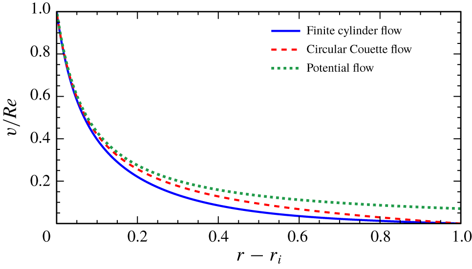
Radial profiles of the azimuthal velocity at  $z=0$ (mid-height) for the finite-cylinder flow at
 $\unicode[STIX]{x1D702}=0.07$,
 $\unicode[STIX]{x1D6FE}=1$,
 $\unicode[STIX]{x1D70E}=6$,
 $Gr=4\times 10^{10}$,
 $\unicode[STIX]{x1D716}=0.064$ and
 $Re\in [1,6000]$ (profiles scaled with
 $Re$ all collapse onto the one curve), the circular Couette flow profile (3.1) and the potential flow profile
 $v(r)/Re=r_{i}/r$.

Figure 2 shows the numerically computed profiles (solid blue curve) of  $v(r)/Re$ at the cylinder mid-height (
 $z=0$) of the steady axisymmetric basic state for twelve values of the Reynolds number in the range
 $Re\in [1,6000]$, all with
 $\unicode[STIX]{x1D702}=0.07$,
 $\unicode[STIX]{x1D6FE}=1$,
 $\unicode[STIX]{x1D70E}=6$,
 $Gr=4\times 10^{10}$ and
 $\unicode[STIX]{x1D716}=0.064$. The differences in the profiles for different
 $Re$ only modify the velocity by one part in
 $10^{5}$, and so the profiles collapse onto the same (blue) curve. Also included in the figure for comparison are the profiles corresponding to the idealized infinite-cylinder circular Couette profile (3.1) and the potential vortex profile
 $v(r)/Re=r_{i}/r$. The circular Couette flow and the potential flow have no meridional flow, i.e.
 $u=w=\unicode[STIX]{x1D714}_{r}=\unicode[STIX]{x1D714}_{\unicode[STIX]{x1D703}}=0$, while
 $v$ and
 $\unicode[STIX]{x1D714}_{z}$ are linear in
 $Re$;
 $\unicode[STIX]{x1D714}_{z}=-2\unicode[STIX]{x1D702}Re/(1+\unicode[STIX]{x1D702})$ is constant for the circular Couette flow, and
 $\unicode[STIX]{x1D714}_{z}=0$ for the potential flow. The numerical simulations of the finite-cylinder problem agree qualitatively with the experimental results reported in figure 6(b) of Riedinger et al. (Reference Riedinger, Le Dizès and Meunier2011), even though they had a rectangular container instead of a circular outer cylinder. In summary, for all basic states (potential flow, circular Couette and finite length cylinder), the primary flow (azimuthal velocity and axial vorticity) scales linearly with Reynolds number:
 $v\propto Re$ and
 $\unicode[STIX]{x1D714}_{z}\propto Re$.
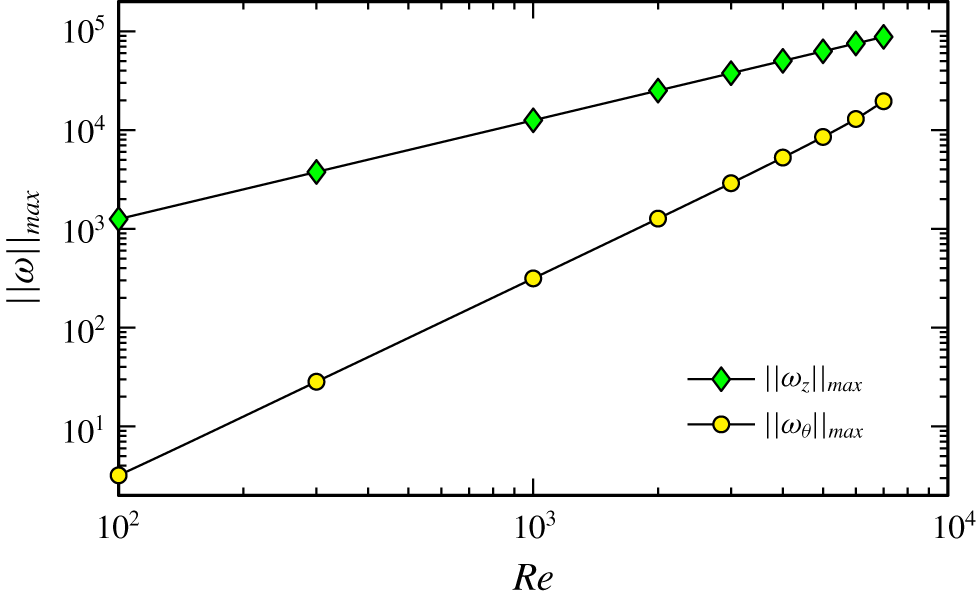
Variation of the maximum in the axial and azimuthal vorticity components with  $Re$, for
 $\unicode[STIX]{x1D702}=0.07$,
 $\unicode[STIX]{x1D6FE}=1$,
 $\unicode[STIX]{x1D70E}=6$,
 $Gr=4\times 10^{10}$ and
 $\unicode[STIX]{x1D716}=0.064$.

The primary flow consists of the azimuthal velocity  $v$ (the only non-zero component in the potential flow and circular Couette flow) and the axial component of vorticity
 $\unicode[STIX]{x1D714}_{z}$ (the only non-zero component in circular Couette flow). With a finite cylinder, a secondary meridional flow is driven by vortex line bending due to the nonlinear advection term and the no-slip velocity boundary conditions at the top and bottom endwalls. As a result,
 $u$,
 $w$,
 $\unicode[STIX]{x1D714}_{r}$ and
 $\unicode[STIX]{x1D714}_{\unicode[STIX]{x1D703}}$ are non-zero. Figure 3 shows how the primary and meridional components of the finite-cylinder flow scale with
 $Re$, where we have used the global maxima of
 $\unicode[STIX]{x1D714}_{z}$ and
 $\unicode[STIX]{x1D714}_{\unicode[STIX]{x1D703}}$ to characterize the primary and meridional components, respectively. For very small
 $Re$,
 $\unicode[STIX]{x1D714}_{\unicode[STIX]{x1D703}}$ is orders of magnitude smaller than
 $\unicode[STIX]{x1D714}_{z}$, but
 $\unicode[STIX]{x1D714}_{z}$ only grows linearly with
 $Re$ whereas
 $\unicode[STIX]{x1D714}_{\unicode[STIX]{x1D703}}$ grows quadratically with
 $Re$. By
 $Re\approx 6000$, the meridional flow is approximately 17 % of the primary flow, and as will be shown in the following sections, this is the level which leads to instability of the basic state. Note that for small
 $Re$, the velocity and vorticity tend to become orthogonal; they are exactly orthogonal for the circular Couette flow. Also, the helicity density increases with increasing
 $Re$. Ignoring centrifugal buoyancy (
 $\unicode[STIX]{x1D716}=0$), the helicity (volume integral of the helicity density) vanishes due to the
 ${\mathcal{K}}$ reflection invariance of the flow, but with
 $\unicode[STIX]{x1D716}\neq 0$ the helicity does not vanish.
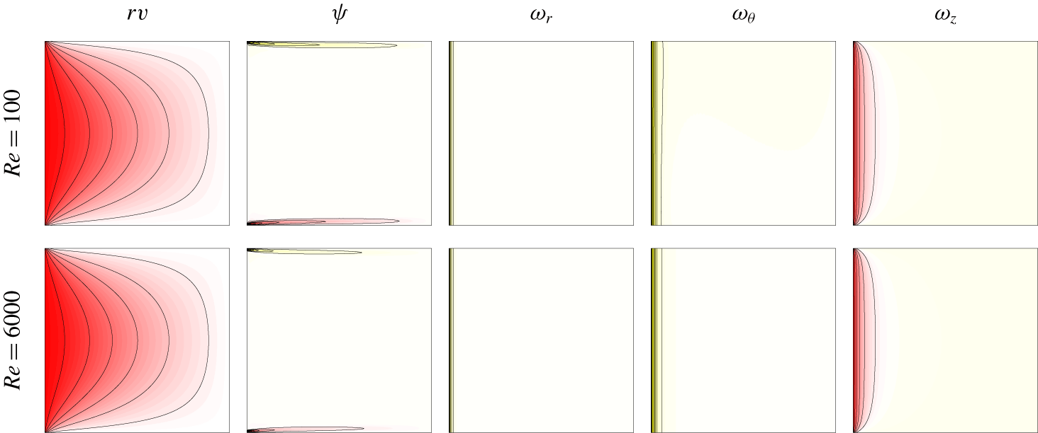
Vortex lines  $rv$, streamlines
 $\unicode[STIX]{x1D713}$ and the three components of vorticity
 $\unicode[STIX]{x1D714}_{r}$,
 $\unicode[STIX]{x1D714}_{\unicode[STIX]{x1D703}}$ and
 $\unicode[STIX]{x1D714}_{z}$ for the basic state at
 $Re$ as indicated. Eight contours are shown, equispaced between the minimum and maximum values of the variables. Parameter values:
 $\unicode[STIX]{x1D702}=0.07$,
 $\unicode[STIX]{x1D6FE}=1$,
 $\unicode[STIX]{x1D70E}=6$,
 $Gr=4\times 10^{10}$ and
 $\unicode[STIX]{x1D716}=0.064$.

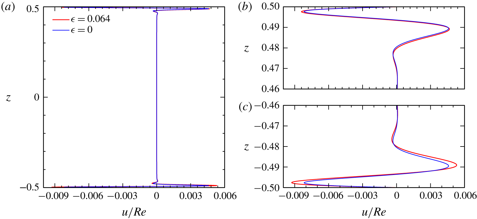
(a) Vertical profiles of the radial velocity near the rotating inner cylinder at $r=r_{i}+0.011$, for the basic state with centrifugal buoyancy (
 $\unicode[STIX]{x1D716}=0.064$, blue) and without (
 $\unicode[STIX]{x1D716}=0$, red), and (b,c) close ups of the profiles near the top and bottom endwalls. Parameter values:
 $\unicode[STIX]{x1D702}=0.07$,
 $\unicode[STIX]{x1D6FE}=1$,
 $\unicode[STIX]{x1D70E}=6$,
 $Gr=4\times 10^{10}$ and
 $Re=6000$.

Figure 4 shows contours of angular momentum  $rv$, streamfunction
 $\unicode[STIX]{x1D713}$ (where
 $[\unicode[STIX]{x2202}^{2}/\unicode[STIX]{x2202}z^{2}+\unicode[STIX]{x2202}^{2}/\unicode[STIX]{x2202}r^{2}-1/r\,\unicode[STIX]{x2202}/\unicode[STIX]{x2202}r]\unicode[STIX]{x1D713}=-r\unicode[STIX]{x1D714}_{\unicode[STIX]{x1D703}}$), and the three components of vorticity at
 $Re=100$ and
 $Re=6000$. The differences in the spatial structures at the two
 $Re$ values are minimal, (except for the scalings in
 $Re$, linear for the primary flow components and quadratic for the meridional components), and localized at the inner wall and endwalls. The vorticity is concentrated in a thin boundary layer at the inner cylinder wall. The thickness of this boundary layer is independent of
 $Re$, but its intensity scales linearly with
 $Re$ (dominated by the contribution from
 $\unicode[STIX]{x1D714}_{z}$). The large-scale circulation induced by the secondary flow is localized in thin endwall boundary layers, as illustrated by the streamfunction contours in figure 4. This is due to the strong stable vertical temperature gradient inhibiting the vertical motion of the fluid outside of boundary layers. There is also a weak breaking of the reflection symmetry
 ${\mathcal{K}}$ due to the centrifugal buoyancy (
 $\unicode[STIX]{x1D716}=0.064$). In order to quantify the intensity of the secondary flow and the symmetry breaking, we have plotted in figure 5 vertical profiles of the radial velocity near the inner cylinder (at
 $r=r_{i}+0.011$, where
 $u(r)$ is maximal), for the basic states with and without the centrifugal term, at
 $Re=6000$. The secondary flow is confined near the top and bottom endwalls, in agreement with the
 $\unicode[STIX]{x1D713}$ contours shown in figure 4, and the maximum of
 $u$ is approximately 0.9 % of the maximum of the primary flow (which is
 $v_{max}=Re$). The solution without centrifugal buoyancy (
 $\unicode[STIX]{x1D716}=0$, blue curve), is
 ${\mathcal{K}}$ reflection symmetric, while the solution including centrifugal buoyancy (
 $\unicode[STIX]{x1D716}=0.064$, red curve), is not. The secondary circulation is more intense near the bottom when
 $\unicode[STIX]{x1D716}\neq 0$, due to centrifugal buoyancy, with the maximum value of
 $u$ in the bottom boundary layer approximately 10 % larger than the maximum value of
 $u$ in the top boundary layer. This is a measure of the symmetry breaking due to the centrifugal effect on the secondary flow, for the basic state at
 $Re=6000$.
4 Helical rotating wave instabilities ignoring centrifugal buoyancy
The basic state, either with or without centrifugal buoyancy effects being considered, loses stability as  $Re$ is increased beyond approximately 6000 for the radius ratio
 $\unicode[STIX]{x1D702}=0.07$, aspect ratio
 $\unicode[STIX]{x1D6FE}=1$, Prandtl number
 $\unicode[STIX]{x1D70E}=6$ and Grashof number
 $Gr=4\times 10^{10}$ considered in this study. Although the basic states with (
 $\unicode[STIX]{x1D716}=0.064$) and without (
 $\unicode[STIX]{x1D716}=0$) buoyancy effects only differ slightly, as described in the previous section, the differences in their instabilities are significant. We begin by describing the instabilities ignoring buoyancy effects in this section, and then in the next section we explore the consequences of including them.
Neglecting buoyancy effects ( $\unicode[STIX]{x1D716}=0$) endows the system with the additional symmetry
 ${\mathcal{K}}$, the invariance to reflection about the annular mid-height. As described in § 2.1, the
 $\unicode[STIX]{x1D716}=0$ system and its basic state have
 $SO(2)\times Z_{2}$ symmetry. Bifurcations from the basic state may either preserve or break parts or all of the symmetries. As in the experiments of Riedinger et al. (Reference Riedinger, Le Dizès and Meunier2011) and Flór et al. (Reference Flór, Hirschberg, Oostenrijk and van Heijst2018), the basic state becomes unstable via a Hopf bifurcation that breaks the
 $SO(2)$ axisymmetry. Generically,
 $SO(2)$ symmetry is broken via a Hopf bifurcation and the resulting limit cycle is a rotating wave with azimuthal wavenumber
 $m$ (Marques & Lopez Reference Marques and Lopez2006). Also in agreement with the experiments, we find that
 $m=1$. The limit cycle consists of two helical waves, one directed downward and the other upward, which combine to form a standing helical wave, with the property of being a rotating wave (RW)
 $$\begin{eqnarray}{\mathcal{R}}_{-\unicode[STIX]{x1D6FD}}\text{RW}(t)=\text{RW}(t+\unicode[STIX]{x1D70F}\unicode[STIX]{x1D6FD}/2\unicode[STIX]{x03C0}),\end{eqnarray}$$
where  $\unicode[STIX]{x1D70F}$ is the period of the rotating wave. Note that for an
 $m=1$ rotating wave, advancing half a period is equivalent to a
 $\unicode[STIX]{x03C0}$ rotation:
 ${\mathcal{R}}_{\unicode[STIX]{x03C0}}\,\text{RW}(t)=\text{RW}(t+\unicode[STIX]{x1D70F}/2)$. The reflection symmetry
 ${\mathcal{K}}$ may either be preserved or broken at the Hopf bifurcation. If it is preserved, the rotating wave is pointwise invariant and we shall denote it
 $\text{RW}_{{\mathcal{K}}}$. It has the property that applying
 ${\mathcal{K}}$ at any point in time leaves it invariant:
 $$\begin{eqnarray}{\mathcal{K}}\text{RW}_{{\mathcal{K}}}(t)=\text{RW}_{{\mathcal{K}}}(t).\end{eqnarray}$$
If the  ${\mathcal{K}}$ reflection is broken at the Hopf bifurcation, the rotating wave is setwise invariant and we shall denote it
 $\text{RW}_{{\mathcal{C}}}$. At any instant in time, reflecting
 $\text{RW}_{{\mathcal{C}}}$ results in
 $\text{RW}_{{\mathcal{C}}}$ half a period later
 $$\begin{eqnarray}{\mathcal{K}}\text{RW}_{{\mathcal{C}}}(t)=\text{RW}_{{\mathcal{C}}}(t+\unicode[STIX]{x1D70F}/2).\end{eqnarray}$$
However, as noted above, for an  $m=1$ rotating wave, advancing half a period is the same as applying a rotation of angle
 $\unicode[STIX]{x03C0}$,
 ${\mathcal{R}}_{\unicode[STIX]{x03C0}}$. Therefore
 $\text{RW}_{{\mathcal{C}}}$ is also pointwise invariant, but with respect to the centrosymmetry
 ${\mathcal{C}}$, whose action is
 $$\begin{eqnarray}{\mathcal{C}}:[u,v,w,T](r,\unicode[STIX]{x1D703},z,t)\mapsto [u,v,-w,-T](r,\unicode[STIX]{x1D703}-\unicode[STIX]{x03C0},-z,t),\end{eqnarray}$$
so that
 $$\begin{eqnarray}{\mathcal{C}}\text{RW}_{{\mathcal{C}}}(t)={\mathcal{R}}_{\unicode[STIX]{x03C0}}{\mathcal{K}}\text{RW}_{{\mathcal{C}}}(t)={\mathcal{R}}_{\unicode[STIX]{x03C0}}\text{RW}_{{\mathcal{C}}}(t+\unicode[STIX]{x1D70F}/2)=\text{RW}_{{\mathcal{C}}}(t).\end{eqnarray}$$
The centrosymmetry  ${\mathcal{C}}$ consists of a rotation of
 $\unicode[STIX]{x03C0}$ around the cylinder axis composed with the
 ${\mathcal{K}}$ reflection:
 ${\mathcal{C}}={\mathcal{R}}_{\unicode[STIX]{x03C0}}{\mathcal{K}}$. It can also be thought of as a reflection through the origin, and since
 ${\mathcal{C}}^{2}$ is the identity, like
 ${\mathcal{K}}$ it also generates a
 $Z_{2}$ group.
As with  $\text{RW}_{{\mathcal{K}}}$,
 $\text{RW}_{{\mathcal{C}}}$ also consists of two helical waves, one directed down and the other up, which combine to form a standing helical wave, with the property of being a rotating wave;
 $\text{RW}_{{\mathcal{K}}}$ and
 $\text{RW}_{{\mathcal{C}}}$ look quite similar, but a clear distinction is that
 $\text{RW}_{{\mathcal{K}}}$ and
 $\text{RW}_{{\mathcal{C}}}$ have opposite parities in
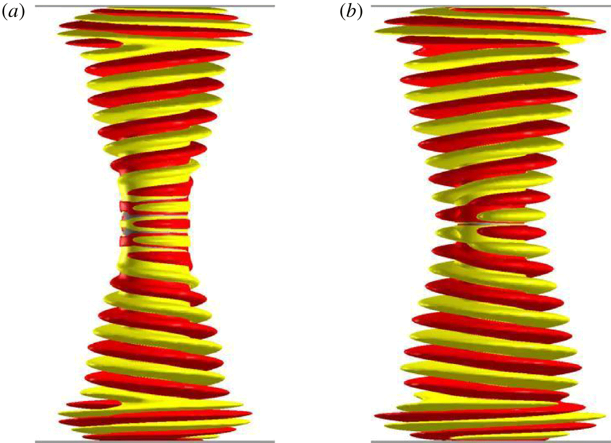
 $z$. Figure 6 shows an example of each, using isocontours of the helicity density. Supplementary movie 1 (available at https://doi.org/10.1017/jfm.2020.135) animates them, illustrating their rotating wave spatio-temporal structure.
Isosurfaces of helicity density at levels  $He=\pm 10^{6}$ for rotating helical wave states (a)
 $\text{RW}_{{\mathcal{C}}}$ at
 $Re=6150$ and (b)
 $\text{RW}_{{\mathcal{K}}}$ at
 $Re=6250$, both with
 $\unicode[STIX]{x1D716}=0$ (no centrifugal buoyancy),
 $Gr=4\times 10^{10}$,
 $\unicode[STIX]{x1D70E}=6$,
 $\unicode[STIX]{x1D702}=0.07$ and
 $\unicode[STIX]{x1D6FE}=1$. The grey disks drawn at the top and bottom endwalls have radii
 $r_{i}+0.2$, i.e. they extend out to 20 % of the radial gap. Supplementary movie 1 animates both.

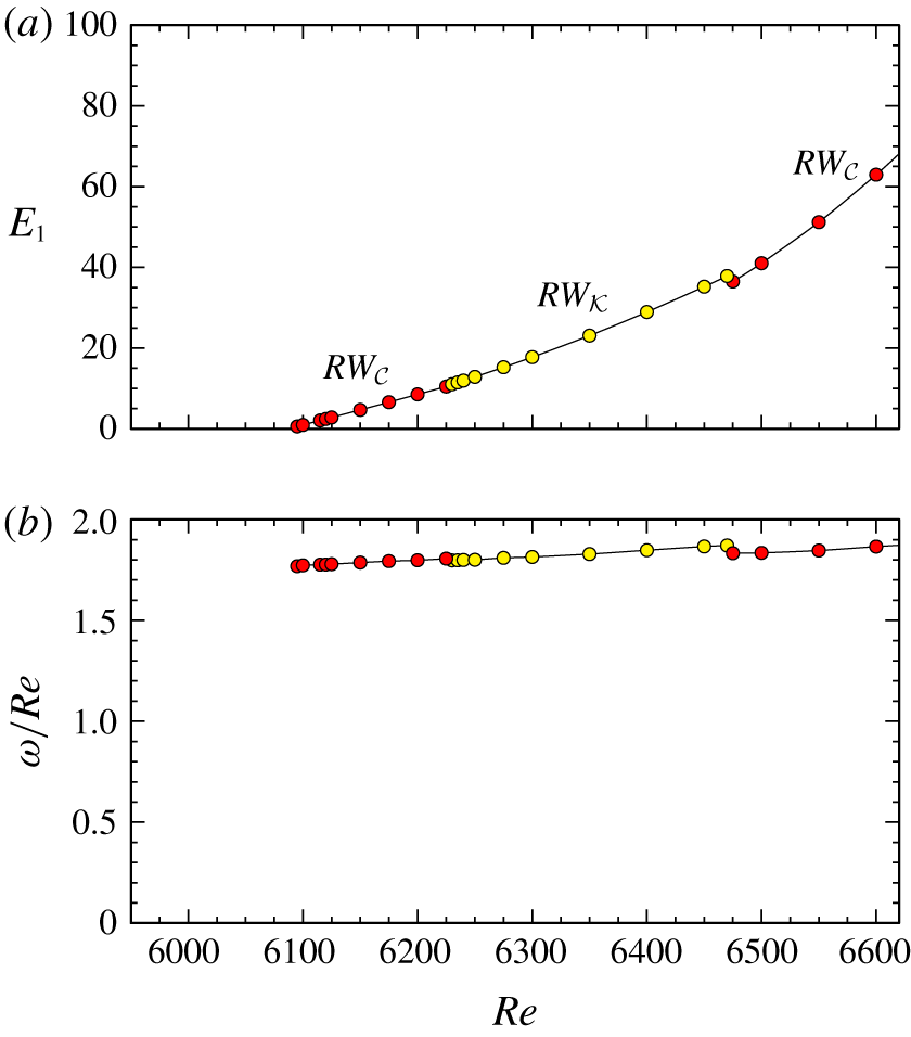
Variation with  $Re$ of (a) the modal energy
 $E_{1}$ and (b) angular frequency (scaled by
 $Re$) of the rotating waves
 $\text{RW}_{{\mathcal{C}}}$ and
 $\text{RW}_{{\mathcal{K}}}$ for
 $\unicode[STIX]{x1D702}=0.07$,
 $\unicode[STIX]{x1D6FE}=1$,
 $\unicode[STIX]{x1D70E}=6$,
 $Gr=4\times 10^{10}$ and
 $\unicode[STIX]{x1D716}=0$.

Figure 7(a) is a bifurcation diagram showing the variation of the modal energy  $E_{1}$ with
 $Re$. At
 $Re\approx 6090$, the kinetic energy in azimuthal wavenumber
 $m=1$ begins to grow linearly with increasing
 $Re$, indicative of a supercritical Hopf bifurcation that has broken axisymmetry and spawns a rotating wave. Figure 7(b) shows how the frequency of the bifurcating rotating wave varies with
 $Re$. Note that we present the frequency as
 $\unicode[STIX]{x1D714}/Re$ so that it is in the inertial time scale (
 $\unicode[STIX]{x1D714}$ is the frequency in the viscous time scale used to compute the flow). In the inertial time scale, the frequency
 $\unicode[STIX]{x1D714}/Re\approx 1.8$ with very little variation with
 $Re$. The two possible types of bifurcating rotating waves,
 $\text{RW}_{{\mathcal{K}}}$ and
 $\text{RW}_{{\mathcal{C}}}$, are stable in different
 $Re$ ranges, and change from one to the other. This is likely due to the fact that these rotating waves are the result of the interaction of two helical waves originating at the corners where the rotating inner cylinder meets the top and bottom endwalls, and grow axially inward with increasing
 $Re$ and interact at the cylinder mid-height (
 $z=0$), where the helical waves have the smallest intensity. Therefore the resulting rotating waves and their stability are very sensitive to small changes, and in particular to the variation with
 $Re$. The energy
 $E_{1}$ and the frequency
 $\unicode[STIX]{x1D714}/Re$ change continuously with
 $Re$, regardless of the solution type. In the parameter regime considered,
 $\text{RW}_{{\mathcal{C}}}$ bifurcates first, and after a relative change in
 $Re$ of approximately 1.7 %,
 $\text{RW}_{{\mathcal{K}}}$ becomes stable, suggesting that the system is close to a double-Hopf bifurcation where the two states with different symmetries,
 $\text{RW}_{{\mathcal{C}}}$ and
 $\text{RW}_{{\mathcal{K}}}$, bifurcate simultaneously. Nevertheless, these symmetry-related peculiarities are a direct consequence of ignoring the centrifugal buoyancy.
5 Centrifugal buoyancy effects on the instabilities
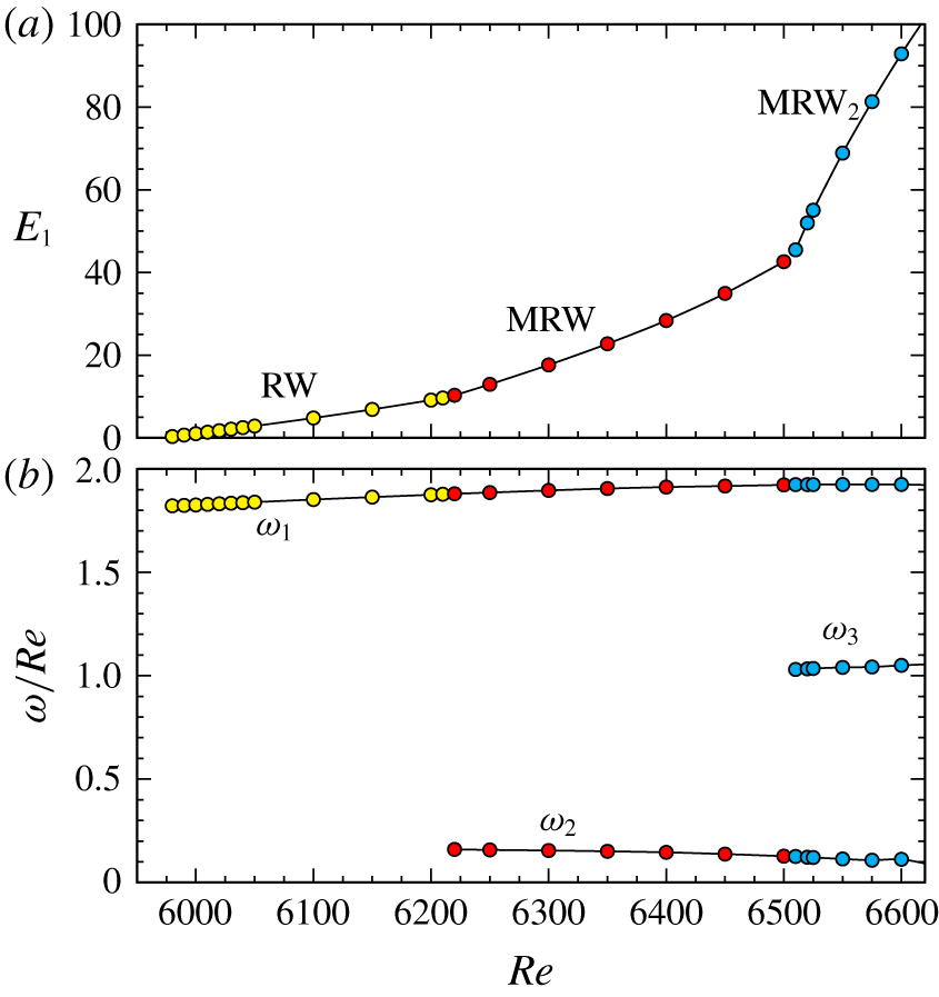
Variation with  $Re$ of (a) the modal energy
 $E_{1}$ and (b) frequencies (scaled by
 $Re$) of rotating wave RW and modulated rotating waves MRW and
 $\text{MRW}_{2}$ (time-averaged
 $E_{1}$ is shown for MRW and
 $\text{MRW}_{2}$), for
 $\unicode[STIX]{x1D702}=0.07$,
 $\unicode[STIX]{x1D6FE}=1$,
 $\unicode[STIX]{x1D70E}=6$,
 $Gr=4\times 10^{10}$ and
 $\unicode[STIX]{x1D716}=0.064$.

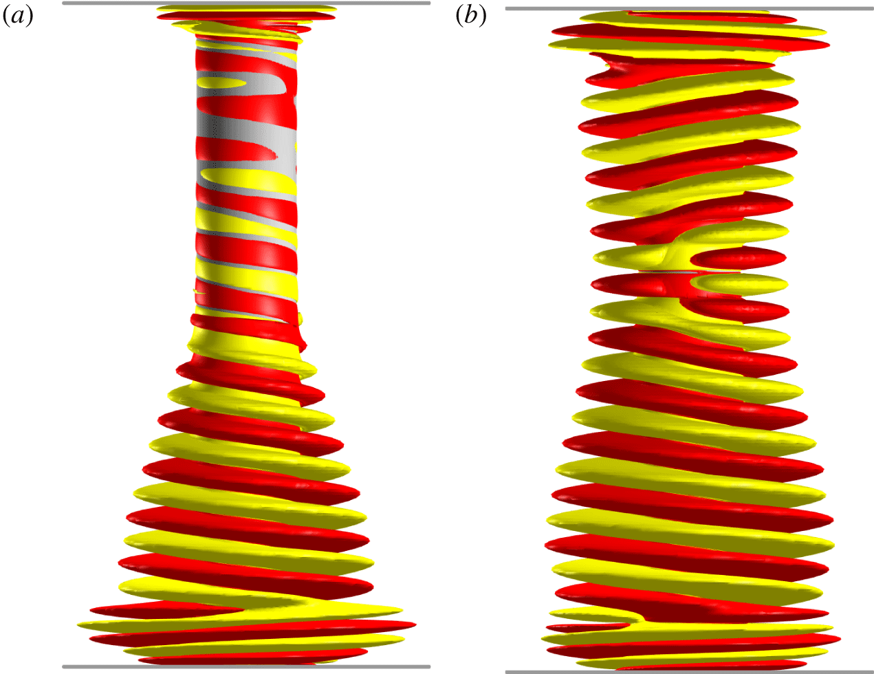
Isosurfaces of helicity density for (a) RW at  $Re=6100$ and (b) MRW at
 $Re=6500$, both with
 $\unicode[STIX]{x1D716}=0.064$ (accounting for centrifugal buoyancy),
 $Gr=4\times 10^{10}$,
 $\unicode[STIX]{x1D70E}=6$,
 $\unicode[STIX]{x1D702}=0.07$ and
 $\unicode[STIX]{x1D6FE}=1$. The isosurface levels are (a)
 $He=\pm 10^{6}$ and (b)
 $He=\pm 3\times 10^{6}$. Supplementary movie 2 animates RW in the inertial frame, and movie 3 animates MRW both in the inertial frame and in a frame rotating at angular frequency
 $\unicode[STIX]{x1D714}_{1}$.

When the centrifugal buoyancy is included in the governing equations (2.1), i.e. taking  $\unicode[STIX]{x1D716}\neq 0$, the system is no longer reflection symmetric, and the symmetry group reduces to
 $SO(2)$. Figure 8 shows the variation of
 $E_{1}$ and the frequencies of the bifurcated states with increasing
 $Re$ when centrifugal buoyancy effects (
 $\unicode[STIX]{x1D716}=0.064$) are taken into account. The basic state undergoes a supercritical Hopf bifurcation to a rotating wave RW with
 $m=1$ and frequency
 $\unicode[STIX]{x1D714}_{1}$. This happens at
 $Re\approx 5970$, which is smaller (approximately 2 %) than the critical
 $Re$ when
 $\unicode[STIX]{x1D716}=0$. The bifurcated state, shown in figure 9(a) at
 $Re=6100$, clearly has no symmetry in
 $z$. The centrifugal buoyancy term drives the denser (colder) fluid near the bottom endwall radially outward, enhancing the centrifugal instability mechanisms near the bottom of the cylinder, while the lighter (hotter) fluid near the top endwall is centrifuged inward, reducing the centrifugal instability. As seen in figure 9(a), the helical wave is generated at the bottom of the cylinder and progresses upwards, while there is no centrifugal instability at the top endwall. Supplementary movie 2 animates the RW shown in figure 9(a).
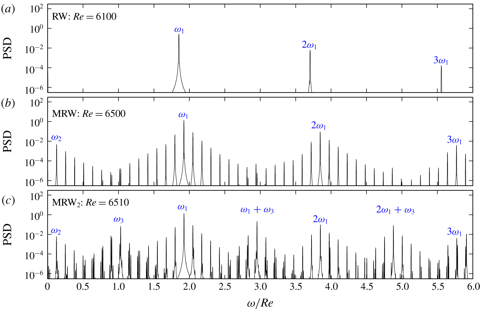
Power spectral density (PSD) of the axial velocity at a point close to the rotating inner cylinder,  $w(r=r_{i}+0.05,\unicode[STIX]{x1D703}=0,z=-0.25)$, for RW, MRW and
 $\text{MRW}_{2}$ at
 $\unicode[STIX]{x1D702}=0.07$,
 $\unicode[STIX]{x1D6FE}=1$,
 $\unicode[STIX]{x1D70E}=6$,
 $Gr=4\times 10^{10}$,
 $\unicode[STIX]{x1D716}=0.064$ and
 $Re$ as indicated.

Snapshots of MRW at  $Re=6500$ in the rotating frame that rotates with angular frequency
 $\unicode[STIX]{x1D714}_{1}$. The time between each snapshot is
 $9.2\times 10^{-4}$ in viscous time units, corresponding to 5.98 inertial time units, so that each set of eight snapshots corresponds to approximately one period of the
 $\unicode[STIX]{x1D714}_{2}$ oscillation (
 $2\unicode[STIX]{x03C0}/\unicode[STIX]{x1D714}_{2}\approx 50.27$). Supplementary movie 3 animates MRW, both in the inertial (laboratory) frame and in the rotating frame.

Increasing the Reynolds number to  $Re\approx 6220$, a helical wave appears at the top of the cylinder. Both helical waves meet near the cylinder mid-plane, but a little closer to the top endwall. In contrast to the two symmetric helical waves of
 $\text{RW}_{{\mathcal{K}}}$ and
 $\text{RW}_{{\mathcal{C}}}$ described earlier with
 $\unicode[STIX]{x1D716}=0$, these two waves are different. The one on the lower half of the cylinder is more intense, and their frequencies are slightly different. They both rotate prograde with the inner cylinder, but the bottom helical wave rotates slightly faster than the top helical wave. This results in a modulated rotating wave state MRW. The difference in the two frequencies shows up as a small beat frequency, which is an order of magnitude smaller than either of the two frequencies. We shall call this beat frequency
 $\unicode[STIX]{x1D714}_{2}$. Figure 10(a) shows the power spectral density (PSD) of the time series obtained from the axial velocity at a point
 $(r,\unicode[STIX]{x1D703},z)=(r_{i}+0.05,0,-0.25)$ of the rotating wave RW at
 $Re=6100$; it consists of
 $\unicode[STIX]{x1D714}_{1}$ and its harmonics. Figure 10(b) is the corresponding PSD of MRW at
 $Re=6500$. It consists of
 $\unicode[STIX]{x1D714}_{1}$ and its harmonics together with
 $\unicode[STIX]{x1D714}_{2}$ and its harmonics. The two frequencies are very close to being commensurate, with
 $\unicode[STIX]{x1D714}_{1}/\unicode[STIX]{x1D714}_{2}\approx 15$; the ‘split’ peaks near
 $0.5\unicode[STIX]{x1D714}_{1}$ and
 $1.5\unicode[STIX]{x1D714}_{1}$ result from their incommensurability. A snapshot of MRW at
 $Re=6500$ is shown in figure 9(b). This state closely resembles the experimental flow obtained by Flór et al. (Reference Flór, Hirschberg, Oostenrijk and van Heijst2018), shown in figure 1(a). Supplementary movie 3 animates MRW, both in the inertial (laboratory) frame and in a frame that rotates with angular frequency
 $\unicode[STIX]{x1D714}_{1}$. In this rotating frame, the helical wave from the bottom is frozen and the helical wave from the top rotates in the retrograde direction at the slow frequency
 $\unicode[STIX]{x1D714}_{2}$; it is a relative rotating wave. There is a torsion between the two behaviours near the mid-height, and this results in a ‘snapping’ between the two helices. A sequence of snapshots of this MRW in the rotating frame at times covering two periods of the
 $\unicode[STIX]{x1D714}_{2}$ oscillation further illustrate this behaviour (see figure 11).
Snapshots of  $\text{MRW}_{2}$ at
 $Re=6510$, in the rotating frame that rotates with angular frequency
 $\unicode[STIX]{x1D714}_{1}$. The time between each snapshot is
 $1.584\times 10^{-4}$ in viscous time units, corresponding to 1.03 inertial time units, so that each set of six snapshots corresponds to approximately one period of the
 $\unicode[STIX]{x1D714}_{3}$ oscillation (
 $2\unicode[STIX]{x03C0}/\unicode[STIX]{x1D714}_{3}\approx 6.16$). Supplementary movie 4 animates
 $\text{MRW}_{2}$, both in the inertial (laboratory) frame and in the rotating frame.

By further increasing the Reynolds number, a more complicated state appears, labelled  $\text{MRW}_{2}$ in figure 8. The PSD of
 $\text{MRW}_{2}$ at
 $Re=6510$ is presented in figure 10(c). A new frequency
 $\unicode[STIX]{x1D714}_{3}$ emerges, which is close to
 $0.5\unicode[STIX]{x1D714}_{1}$, suggestive of a period doubling, but in fact the relationship
 $2\unicode[STIX]{x1D714}_{3}-\unicode[STIX]{x1D714}_{1}\approx \unicode[STIX]{x1D714}_{2}$ is apparent. The detuning in this relationship shows up as a very low frequency beating, with
 $2\unicode[STIX]{x1D714}_{3}-\unicode[STIX]{x1D714}_{1}-\unicode[STIX]{x1D714}_{2}\sim 10^{-2}Re$. Supplementary movie 4 animates
 $\text{MRW}_{2}$ in both the laboratory frame and the rotating frame associated with
 $\unicode[STIX]{x1D714}_{1}$. As with MRW, in the rotating frame the upper part of
 $\text{MRW}_{2}$ has a slow nearly constant rotation, associated with the beat frequency
 $\unicode[STIX]{x1D714}_{2}$. The lower part is essentially not rotating, like the lower part of MRW, but it has a large-scale ‘axisymmetric’ pulsing whose frequency is
 $\unicode[STIX]{x1D714}_{3}$. Figure 12 shows 12 snapshots of
 $\text{MRW}_{2}$ in the
 $\unicode[STIX]{x1D714}_{1}$ rotating frame, covering approximately two
 $\unicode[STIX]{x1D714}_{3}$ periods.
 $\text{MRW}_{2}$ has three incommensurate frequencies, but in the rotating frame it is simply quasi-periodic, a relative two-torus.
6 Discussion and conclusions
The helical instability mode experimentally observed by Flór et al. (Reference Flór, Hirschberg, Oostenrijk and van Heijst2018) when the Froude number  $Fr<1$ in a stratified Taylor–Couette flow with a very wide gap annulus of unit aspect ratio is very different to the instabilities reported in previous experimental investigations of stratified Taylor–Couette flow (e.g. Boubnov, Gledzer & Hopfinger Reference Boubnov, Gledzer and Hopfinger1995; Boubnov et al. Reference Boubnov, Gledzer, Hopfinger and Orlandi1996; Caton, Janiaud & Hopfinger Reference Caton, Janiaud and Hopfinger2000; Le Bars & Le Gal Reference Le Bars and Le Gal2007; Ibanez, Swinney & Rodenborn Reference Ibanez, Swinney and Rodenborn2016; Rüdiger et al. Reference Rüdiger, Seelig, Schultz, Gellert, Egbers and Harlander2017; Seelig, Harlander & Gellert Reference Seelig, Harlander and Gellert2018; Park et al. Reference Park, Billant, Baik and Seo2018). Those other experiments were mostly conducted in the narrow gap regime, with radius ratios in the range
 $\unicode[STIX]{x1D702}\approx 0.8{-}0.9$, with a few considering
 $\unicode[STIX]{x1D702}$ as small as 0.3. These are all considerably larger than the radius ratio of Flór et al. (Reference Flór, Hirschberg, Oostenrijk and van Heijst2018),
 $\unicode[STIX]{x1D702}\approx 0.07$. One consequence of
 $\unicode[STIX]{x1D702}$ being relatively large is that the instability modes fill the entire annular gap. In contrast, the instability in the experiments of Flór et al. (Reference Flór, Hirschberg, Oostenrijk and van Heijst2018) is a helical wave that is very localized to the rotating inner cylinder. The previous stratified Taylor–Couette flow experiments were all conducted using annuli with large height-to-gap aspect ratios, typically with
 $\unicode[STIX]{x1D6FE}$ between 10 and 50. They claim to be motivated to consider large
 $\unicode[STIX]{x1D6FE}$ in order to minimize the effects of endwalls and to try to accommodate the theoretical idealization of a base flow that is unidirectional with instability modes that are axially periodic. The experiment of Flór et al. (Reference Flór, Hirschberg, Oostenrijk and van Heijst2018) had
 $\unicode[STIX]{x1D6FE}\approx 1$. Endwall effects were recognized by them, and they considered the instability to originate at the corners where the rotating cylinder meets the top and bottom. Nevertheless, they concluded their paper with the comment: ‘the dynamics of these waves and the underlying mechanism of the instability remain to be explained’. This is precisely what we have set out to do in this study.
In our simulations, we used parameters that are very close to those of the experiments of Flór et al. (Reference Flór, Hirschberg, Oostenrijk and van Heijst2018), except that we use temperature as the stratifying agent rather than salt. Temperature diffuses approximately 100 times faster than salt, but these molecular processes seem to not be important for the helical instability. That the Prandtl number does not play a major role in the helical wave instability is borne out by the good agreement between our numerical simulations with  $\unicode[STIX]{x1D70E}=6$ and the experiments with Schmidt number of order
 $10^{3}$, further reinforcing our conclusion that the instability is hydrodynamic rather than buoyancy in nature: the vortex line bending at the corners drives a meridional flow which at a critical
 $Re$ becomes unstable to helical waves. Buoyancy of course is relevant; the strong stratification impacts the flow, causing the meridional flow to be localized in thin boundary layers, and then the centrifugal buoyancy results in the flow near the lower corner to lose stability at a lower
 $Re$ than that at the top corner.
For  $\unicode[STIX]{x1D702}=0.07$,
 $\unicode[STIX]{x1D6FE}=1$,
 $\unicode[STIX]{x1D70E}=6$,
 $Gr=4\times 10^{10}$ and
 $\unicode[STIX]{x1D716}=0.064$, we find the critical
 $Re\approx 6\times 10^{3}$. These parameters are very close to those where Flór et al. (Reference Flór, Hirschberg, Oostenrijk and van Heijst2018) experimentally observed the helical instability, which is reproduced in figure 1(a). The helical waves in both their experiment and in our simulations grow from the bottom corner where the rotating cylinder meets the stationary endwall. The azimuthal wavenumber is
 $m=1$ and the axial wavenumber is 14. The axial wavenumber is estimated as in the experiments, by counting the average number of waves over the depth of the annulus. The experimental result reproduced in figure 1(a) is for
 $Re_{i}=Re\,\unicode[STIX]{x1D702}/(1-\unicode[STIX]{x1D702})\approx 521$ and
 $Fr=\unicode[STIX]{x1D6FA}/N=(Re/R_{N})\,(1-\unicode[STIX]{x1D702})/\unicode[STIX]{x1D702}\approx 0.53$. Our critical
 $Re$ corresponds to
 $Re_{i}\approx 451$ and
 $Fr\approx 0.4$. The theoretical stability analysis of the potential flow by Riedinger et al. (Reference Riedinger, Le Dizès and Meunier2011) would suggest that in this parameter regime (
 $Re_{i}\approx 451$ and
 $Fr\approx 0.4$), the potential flow is stable, whereas their experimental results, using a slender rotating cylinder in a large rectangular tank with stably stratified fluid, report an
 $m=1$ helical instability for
 $Re_{i}\approx 450$ and
 $Fr\approx 0.6$. Given the geometric differences between their experiment in a rectangular container and the annular geometry used in Flór et al. (Reference Flór, Hirschberg, Oostenrijk and van Heijst2018) and in the present study, it is quite possible that the instabilities are related.
The frequency of the helical waves at onset is  $\unicode[STIX]{x1D714}_{1}/Re\approx 1.8$ in the inertial time scale, but in the buoyancy time scale it is
 $\unicode[STIX]{x1D714}_{1}/R_{N}\approx 0.054$, which is very small. The linear dispersion relation gives that internal waves would propagate in the linearly stratified medium at an angle inclined to the horizontal of only
 $\unicode[STIX]{x1D6FD}=\arcsin 0.54\approx 3^{\circ }$. We have not observed any significant propagation of internal waves in our simulations. If they are present, they are very weak compared with other flow features and do not play any significant dynamic role in the observed bifurcations.
In the experiments of Flór et al. (Reference Flór, Hirschberg, Oostenrijk and van Heijst2018), since they have the top open, there is no  ${\mathcal{K}}$ reflection symmetry. However, even if the geometry were perfect with the annulus fully enclosed and filled, there is still no
 ${\mathcal{K}}$ symmetry due to centrifugal buoyancy effects. The parameter
 $\unicode[STIX]{x1D716}$ quantifying centrifugal buoyancy is small (approximately 6 % compared to one). We have used
 $\unicode[STIX]{x1D716}=0.064$ in the simulations; this value was estimated to correspond to the experimental case of Flór et al. (Reference Flór, Hirschberg, Oostenrijk and van Heijst2018), reproduced here in figure 1(a). This small number is, however, not small compared to zero, and its effects are dynamically important not just near onset, but beyond as well, eliminating much of the peculiar degeneracies associated with
 ${\mathcal{K}}$ and
 ${\mathcal{C}}$-conjugate states. Similar rationalization of degenerate dynamics resulting from neglecting centrifugal buoyancy has been reported in rotating convection studies (Marques et al. Reference Marques, Mercader, Batiste and Lopez2007; Rubio, Lopez & Marques Reference Rubio, Lopez and Marques2010; Curbelo et al. Reference Curbelo, Lopez, Mancho and Marques2014). In the present problem, centrifugal buoyancy is the explanation for the experimentally observed flow asymmetry. Moreover, accounting for endwall effects is also found to be critical. The instabilities are generated at the corners where the inner cylinder meets the endwalls, rather than uniformly along the inner cylinder. Irrespective of how large the aspect ratio
 $\unicode[STIX]{x1D6FE}$ is made, the endwall effects appear before other instabilities, and propagate toward the cylinder mid-height. As in many other physical realizations of Taylor–Couette flows, even for large
 $\unicode[STIX]{x1D6FE}$, endwall effects cannot be neglected and they generate large-scale dynamics (Benjamin Reference Benjamin1978a,Reference Benjaminb; Benjamin & Mullin Reference Benjamin and Mullin1981; Ahlers & Cannell Reference Ahlers and Cannell1983; Lorenzen, Pfister & Mullin Reference Lorenzen, Pfister and Mullin1983; Cliffe, Kobine & Mullin Reference Cliffe, Kobine and Mullin1992; Lopez, Marques & Shen Reference Lopez, Marques and Shen2000; Czarny et al. Reference Czarny, Serre, Bontoux and Lueptow2002; Abshagen et al. Reference Abshagen, Lopez, Marques and Pfister2005a,Reference Abshagen, Lopez, Marques and Pfisterb, Reference Abshagen, Lopez, Marques and Pfister2008; Avila et al. Reference Avila, Grimes, Lopez and Marques2008; Lopez Reference Lopez2016).
Acknowledgements
This work was supported by the Spanish Ministry of Education and Science/FEDER grants FIS2017-85794-P and PRX18/00179.
Declaration of interests
The authors report no conflict of interest.
Supplementary movies
Supplementary movies are available at https://doi.org/10.1017/jfm.2020.135.