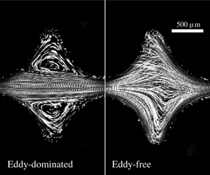
1 Introduction
Polymer solutions have elastic properties that can dramatically alter their flow behaviour in complex geometries. For example, polymer chains can be elongated as they traverse curved streamlines, generating elastic stresses that modify the flow through the formation of recirculating eddies or flow fluctuations over a range of spatial and temporal scales. Such effects are often harnessed to improve oil recovery and groundwater remediation efforts (Roote Reference Roote1998; Sorbie Reference Sorbie2013; Browne, Shih & Datta Reference Browne, Shih and Datta2019). In these cases, an injected polymer solution flows through a tortuous porous medium, such as a reservoir rock or a subsurface aquifer, and displaces trapped non-aqueous fluids from the pore space, enabling them to be recovered downstream. The spatial and temporal characteristics of the pore-scale flow, which typically depend on the medium geometry (Datta et al. Reference Datta, Chiang, Ramakrishnan and Weitz2013; Kang et al. Reference Kang, de Anna, Nunes, Bijeljic, Blunt and Juanes2014; Pak et al. Reference Pak, Butler, Geiger, van Dijke and Sorbie2015; Zami-Pierre et al. Reference Zami-Pierre, De Loubens, Quintard and Davit2016; Blunt Reference Blunt2017), strongly influence this process: for example, local fluctuations in flow speed may generate local increases in the viscous forces that are thought to help displace trapped fluid (Datta, Dupin & Weitz Reference Datta, Dupin and Weitz2014a; Datta, Ramakrishnan & Weitz Reference Datta, Ramakrishnan and Weitz2014b; Clarke et al. Reference Clarke, Howe, Mitchell, Staniland and Hawkes2016; Mitchell et al. Reference Mitchell, Lyons, Howe and Clarke2016). It is therefore critical to be able to predict how the flow behaviour depends on the solution properties, injection conditions, and porous medium geometry. Laboratory and field tests provide key empirical measurements of macroscopic variables including fluid pressure and total recovery (Sandiford et al. Reference Sandiford1964; Durst, Haas & Kaczmar Reference Durst, Haas and Kaczmar1981; Pitts et al. Reference Pitts, Campbell, Surkalo and Wyatt1995; Wang, Wang & Xiaem Reference Wang, Wang and Xia2011a; Vermolen, Van Haasterecht & Masalmeh Reference Vermolen, Van Haasterecht and Masalmeh2014; Wei, Romero-Zerón & Rodrigue Reference Wei, Romero-Zerón and Rodrigue2014). However, broad application is still limited by an incomplete understanding of how these macroscopic variables depend on the pore-scale features of the fluid flow, which in turn depend on polymer properties, pore space geometry, and imposed flow conditions. As a result, the mechanisms underlying polymer solution-enhanced fluid recovery are still widely debated (Chauveteau & Moan Reference Chauveteau and Moan1981; Chauveteau, Moan & Magueur Reference Chauveteau, Moan and Magueur1984; Zaitoun et al. Reference Zaitoun and Kohler1988; Zaitoun, Bertin and Lasseux Reference Zaitoun, Bertin and Lasseux1998; Haward & Odell Reference Haward and Odell2003; Odell & Haward Reference Odell and Haward2006; Huh et al. Reference Huh and Pope2008; Clarke et al. Reference Clarke, Howe, Mitchell, Staniland and Hawkes2016; Mitchell et al. Reference Mitchell, Lyons, Howe and Clarke2016; Browne et al. Reference Browne, Shih and Datta2019), and general principles for predicting and controlling the flow are lacking.
Studies of flow in model microfluidic devices provide valuable insights into the pore-scale flow field. Extensive work has focused on the simplified cases of flow into a single pore constriction or flow into narrow constrictions around a single pillar. In these geometries, the polymer chains are aligned and elongated by the flow, generating upstream recirculating eddies that minimize the extensional stress associated with chain misalignment (Batchelor Reference Batchelor1971; Boger Reference Boger1987; Mongruel & Cloitre Reference Mongruel and Cloitre1995, Reference Mongruel and Cloitre2003; Rodd et al. Reference Rodd, Cooper-White, Boger and McKinley2007). Polymer elongation along the curved fluid streamlines also produces normal elastic stresses, which persist for a duration  $\unicode[STIX]{x1D706}$ before relaxing. Thus, at sufficiently large flow speeds, these stresses build up in the solution, further perturbing the flow and causing an elastic instability to arise: an unsteady flow state develops in which the eddies have a broad spectrum of spatial and temporal fluctuations (Koelling & Prud’homme Reference Koelling and Prud’homme1991; Lanzaro & Yuan Reference Lanzaro and Yuan2011; Kenney et al. Reference Kenney, Poper, Chapagain and Christopher2013; Ribeiro et al. Reference Ribeiro, Coelho, Pinho and Alves2014; Gulati, Muller & Liepmann Reference Gulati, Muller and Liepmann2015; Lanzaro, Li & Yuan Reference Lanzaro, Li and Yuan2015; Shi et al. Reference Shi, Kenney, Chapagain and Christopher2015; Shi & Christopher Reference Shi and Christopher2016; Lanzaro, Corbett & Yuan Reference Lanzaro, Corbett and Yuan2017; Haward, Toda-Peters & Shen Reference Haward, Toda-Peters and Shen2018; Qin et al. Reference Qin, Salipante, Hudson and Arratia2019). A similar instability also arises in other flows with highly curved fluid streamlines (Pearson Reference Pearson1976; Larson Reference Larson1992; McKinley, Pakdel & Öztekin Reference McKinley, Pakdel and Öztekin1996; Pakdel & McKinley Reference Pakdel and McKinley1996; Groisman & Steinberg Reference Groisman and Steinberg2000; Pan et al. Reference Pan, Morozov, Wagner and Arratia2013; Galindo-Rosales et al. Reference Galindo-Rosales, Campo-Deaño, Sousa, Ribeiro, Oliveira, Alves and Pinho2014; Sousa et al. Reference Sousa, Pinho, Oliveira and Alves2015; Haward, McKinley & Shen Reference Haward, McKinley and Shen2016; Qin & Arratia Reference Qin and Arratia2017). However, it is unclear how these effects manifest in a porous medium composed of many successive pore constrictions and expansions, known as throats and bodies, respectively.
Imaging of flow through one-dimensional (1-D) arrays of widely spaced pore throats consistently demonstrates the formation of unstable eddies upstream of each throat, similar to the case of an isolated throat (Khomami & Moreno Reference Khomami and Moreno1997; Arora, Sureshkumar & Khomami Reference Arora, Sureshkumar and Khomami2002; Galindo-Rosales et al. Reference Galindo-Rosales, Campo-Deaño, Pinho, Van Bokhorst, Hamersma, Oliveira and Alves2012; Kenney et al. Reference Kenney, Poper, Chapagain and Christopher2013; Shi et al. Reference Shi, Kenney, Chapagain and Christopher2015; Varshney & Steinberg Reference Varshney and Steinberg2017). By contrast, when the spacing between pore throats is small, chain elongation may persist across multiple pores as the polymers are advected through the pore space. Thus, memory of strain in one pore may influence the flow in a pore further downstream, potentially imparting new spatio-temporal structure to the flow. However, this possibility remains to be explored. Studies conducted at a Reynolds number  $Re\sim 20$ and an elasticity number
 $El\sim 1$, and thus also subject to inertial effects, show that decreasing the spacing between pores produces stronger flow fluctuations (Shi & Christopher Reference Shi and Christopher2016) – providing a clue that polymer memory may indeed influence the flow. Nevertheless, whether and how polymer memory impacts flow through a porous medium has not been fully resolved for the case of
 $Re\ll 1$ and
 $El\gg 1$, in which elastic effects dominate and inertial effects do not also arise. This flow regime is particularly relevant to key applications including oil recovery and groundwater remediation, which can have
 $Re$ ranging from
 ${\sim}10^{-11}$ to
 $10^{-3}$ and
 $El$ ranging from
 ${\sim}10^{2}$ to
 $10^{11}$.
Here, we use confocal microscopy to investigate the unstable flow of an elastic polymer solution through a 1-D ordered array of pores at  $Re\ll 1$ and
 $El\gg 1$. This model geometry provides a way to systematically vary the spacing between pores, enabling us to isolate and directly test the relative importance of polymer memory on the flow behaviour. When the spacing between pores is large, unstable eddies form upstream of each throat, similar to observations of an isolated throat. By contrast, when the spacing between pores is sufficiently small, the flow exhibits a surprising bistability. In each pore body, the flow persists over long durations in one of two distinct flow states: an eddy-dominated state in which a pair of large unstable eddies forms in the corners of the pore body, and an eddy-free state in which strongly fluctuating fluid pathlines fill the entire pore body and eddies do not form. We hypothesize that this unusual behaviour arises from the interplay between flow-induced polymer elongation, which promotes eddy formation, and relaxation of polymers as they are advected between pores, which enables the eddy-free state to form. Consistent with this idea, we find that the flow state in a given pore persists for long times. In addition, we find that the instantaneous flow state is correlated between neighbouring pores; however, these correlations do not persist over long times. Thus, our results reveal that the characteristics of unstable flow are not determined just by injection conditions and the geometry of the individual pores, but also depend on the spacing between pores. Ultimately, these results help to elucidate the rich array of behaviours that can arise in polymer solution flow through porous media.
2 Materials and methods
The void space of a porous medium is typically composed of successive expansions known as pore bodies connected by narrower constrictions known as pore throats (Doyen Reference Doyen1988; Kwiecien, Macdonald & Dullien Reference Kwiecien, Macdonald and Dullien1990; Bernabe Reference Bernabe1991; Ioannidis & Chatzis Reference Ioannidis and Chatzis1993). We use three-dimensional (3-D) printing to make model porous media that recapitulate these geometric features (O’Connell et al. Reference O’Connell, Lu, Browne and Datta2019). Importantly, this approach provides precise control over the pore space geometry, and yields devices that can be optically interrogated while also withstanding the high pressures that arise during elastic polymer solution flow.
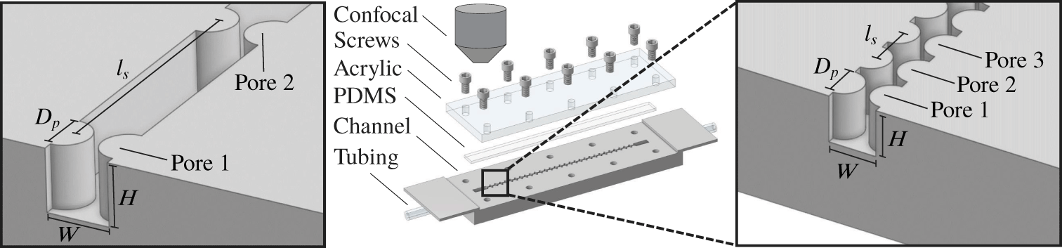
The media are made of straight, square channels having constrictions defined by evenly spaced hemi-cylindrical posts, as illustrated in figure 1. For simplicity, this geometry thus does not incorporate complex pore space tortuosity and connectivity; instead, it provides a way to isolate and systematically probe the role of pore spacing on flow behaviour. Each channel is  $W=2~\text{mm}$ wide,
 $H=2~\text{mm}$ high and 7 cm long, with opposing posts of diameter
 $D_{p}=1.6~\text{mm}$ that are laterally separated by
 $L_{c}=0.4~\text{mm}$ and spaced by a centre-to-centre distance of
 $l_{s}$ along the flow direction. The space between hemi-cylinders along the flow direction thus defines the pore bodies, while the lateral constriction between opposing hemi-cylinders defines the pore throats. Varying
 $l_{s}$ provides a way to systematically test the influence of pore spacing on the flow; hence, our experiments probe an isolated pore throat with
 $l_{s}\rightarrow \infty$, a pair of throats with
 $l_{s}=16W$, and an array of 30 throats with
 $l_{s}=1W$.
Experimental set-up. Fluidic channel contains pore throat constrictions defined by opposing hemi-cylindrical posts and is fabricated using a stereolithographic 3-D printer. Dimensions are  $W=2~\text{mm}$,
 $H=2~\text{mm}$,
 $D_{p}=1.6~\text{mm}$. We vary the pore throat separation distance
 $l_{s}$ and the number of throats in the channel (two examples are shown in the left and right panels). The channel is screwed shut with an acrylic plate over a thin strip of PDMS. Inlet and outlet tubing is glued into 3-D printed holes. The set-up is inverted and videos are captured on a confocal microscope; the middle panel is vertically flipped for clarity.

To fabricate each device, we 3-D print the open-faced channel with a FormLabs Form 2 stereolithography printer, using a proprietary clear polymeric resin (FLGPCL04) composed of methacrylate oligomers and photoinitiators. We then glue inlet and outlet tubing directly into 3-D printed connectors designed to minimize perturbation of the polymers away from the pores. Finally, as shown in figure 1, the whole assembly is screwed shut using a clear acrylic sheet laser cut to size and placed on top of a thin strip of polydimethylsiloxane (PDMS), which provides a watertight seal.
The fluid used is an aqueous solution of 18 MDa partially hydrolyzed polyacrylamide (HPAM, 30 % carboxylated monomers; Polysciences), a polymer commonly used in oil recovery (Sandiford et al. Reference Sandiford1964; Wei et al. Reference Wei, Romero-Zerón and Rodrigue2014). We dissolve 300 ppm HPAM in a solvent of 10 vol% ultrapure water (Millipore) and 90 vol% glycerol (Sigma Aldrich) containing 1 wt% NaCl (Sigma Aldrich). We use dynamic light scattering to directly measure the mean polymer radius of gyration  $R_{g}$ for a dilute solution of 30 ppm HPAM in the same solvent mixture used in the flow experiments. We find
 $R_{g}\approx 196$ nm; furthermore, we estimate the polymer overlap concentration via the relation
 $C^{\ast }\approx (M_{w}/V)/N_{A}$, where
 $M_{w}$ is the polymer molecular weight,
 $V=4\unicode[STIX]{x03C0}R_{g}^{3}/3$ is the volume occupied by a single polymer molecule, and
 $N_{A}$ is Avogadro’s number (Rubinstein & Colby Reference Rubinstein and Colby2003). This calculation yields an overlap concentration of
 $C^{\ast }\approx 940~\text{ppm}$ and therefore our experiments use a dilute polymer solution at
 ${\approx}0.3$ the overlap concentration. We also seed the polymer solution with 1 ppm of fluorescent
 $1~\unicode[STIX]{x03BC}\text{m}$ polystyrene tracer particles (Invitrogen) to enable flow visualization; the particles have excitation between 480 and 510 nm with an excitation peak at 505 nm, and emission between 505 and 540 nm with an emission peak at 515 nm. For each medium geometry tested, we prepare a fresh solution and use it within one month.
The channel dimensions and polymer concentration used in our experiments enable us to isolate the influence of polymer elongation and relaxation between pores, with a minimal influence of polymer surface adsorption, flow-induced chain migration, wall slip, shear banding and polymer entanglement. As described further in the Appendix, we expect that polymer adsorption, migration and wall slip occur over length scales  ${\sim}0.1$ to
 $10~\unicode[STIX]{x03BC}\text{m}$, over one to three orders of magnitude smaller than the smallest channel dimension
 $L_{c}=400~\unicode[STIX]{x03BC}\text{m}$. Also, as described further in the Appendix, we expect that shear banding and polymer entanglement effects do not occur for the dilute concentrations explore here. However, such effects could play a role in the flow of more concentrated polymer solutions in media with smaller pores.
To visualize the flow, we invert and mount each assembled device on a Nikon A1R inverted laser-scanning confocal microscope. The polymer solution is subsequently injected through the porous medium at a fixed volumetric flow rate  $Q$ using a syringe pump (Harvard Apparatus PHD 2000). The time required to inject a single pore throat volume is then given by
 $\unicode[STIX]{x1D70F}_{pv}\equiv V_{pv}/Q$, where we define the pore throat volume as the void volume between the beginning and end of a pair of opposing hemi-cylinders,
 $V_{pv}=D_{p}WH-\unicode[STIX]{x03C0}D_{p}^{2}H/4$. In our experiments at sufficiently large
 $Q$, we find that unstable fluctuations begin after
 ${\approx}10\unicode[STIX]{x1D70F}_{pv}$ and continue to develop over a time scale of
 ${\approx}40\unicode[STIX]{x1D70F}_{pv}$, after which it reaches a dynamic equilibrium in which the statistical properties of the flow, described in § 3, do not appreciably change. Our flow visualization measurements are thus taken
 ${\approx}300\unicode[STIX]{x1D70F}_{pv}$ after initiating the flow to ensure that the unstable state is fully developed. For imaging, we use a green laser with an excitation wavelength of 488 nm and detection in the range 500–550 nm, which enables us to identify the individual fluorescent particles. We employ resonant scanning, in which the laser is raster scanned over each pixel sequentially, with a CFI60 Plan Apochromat Lambda 4X objective lens with 0.2 numerical aperture. This set-up enables us to continually raster a field of view of
 $2127~\unicode[STIX]{x03BC}\text{m}$ by
 $2127~\unicode[STIX]{x03BC}\text{m}$. We acquire fluorescence images every 33 ms, or at 30 frames per second, from an optical slice of
 $17.9~\unicode[STIX]{x03BC}\text{m}$ thickness in the centre of the channel height. To visualize the pathlines of the individual tracer particles, we average successive frames for
 $10\unicode[STIX]{x1D70F}_{pv}$, yielding the micrographs shown hereafter.
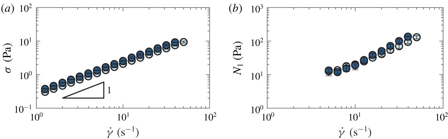
We characterize the solution rheology using an Anton Paar MCR-501 rheometer with a  $50~\text{mm}~1^{\circ }$ cone-plate geometry. Figure 2 shows the measured shear stress
 $\unicode[STIX]{x1D70E}$ and first normal stress difference
 $N_{1}$ over different shear rates
 $\dot{\unicode[STIX]{x1D6FE}}$ for a representative solution. Furthermore, to assess possible degradation of polymers due to unstable flow in the porous media (Vanapalli, Ceccio & Solomon Reference Vanapalli, Ceccio and Solomon2006), we also measure the solution rheology after performing flow experiments at the highest flow rates tested. We find no significant difference between the solution rheology measured before (dark blue points in figure 2) and after (light blue points) flow experiments, indicating minimal polymer degradation due to the unstable flow. For each solution used in each experiment, we obtain at least five replicate measurements of the fluid rheology and use the averaged values in all subsequent calculations.
Rheology of HPAM polymer solutions. Panel (a) shows the shear stress  $\unicode[STIX]{x1D70E}$ and panel (b) shows the first normal stress difference
 $N_{1}$ as functions of the shear rate
 $\dot{\unicode[STIX]{x1D6FE}}$ for the sample used for figures 4(c), 6, 7 and 8(b–d). Data are taken before (dark blue) and after (light blue) a porous media flow experiment, showing that polymers are not appreciably degraded by the unstable flow. Error bars represent standard deviation over five replicate rheological measurements. Fresh polymer solutions are prepared for each experiment, and all dimensionless quantities described in the text are calculated using rheology on fresh samples.

The shear stress varies approximately linearly with shear rate, with a shear thinning exponent  ${\approx}0.92$, indicating that shear thinning effects are small due to the high viscosity of the background solvent. Indeed, the pure solvent viscosity is approximately 0.6 times the measured solution viscosity. However, for accuracy, we use the rate-dependent shear viscosity
 $\unicode[STIX]{x1D707}(\dot{\unicode[STIX]{x1D6FE}})\equiv \unicode[STIX]{x1D70E}(\dot{\unicode[STIX]{x1D6FE}})/\dot{\unicode[STIX]{x1D6FE}}$ in all calculations. The shear rate varies widely within the complex geometry used in our experiments; therefore, to determine a shear rate that characterizes each experiment, we evaluate the wall shear rate in the pore throat at each value of
 $Q$ tested, since it is the maximal shear rate in our system. We do this using the flow profile for a non-Newtonian fluid having the measured shear-thinning exponent 0.92, as calculated by Harnett & Irvine (Reference Harnett and Irvine1979) and by Son (Reference Son2007). We use this choice of the maximal shear rate to estimate characteristic values of the fluid Reynolds number, Weissenberg number, elasticity number and the
 $M$ parameter, as described further below. In particular, this choice of wall shear rate enables us to provide upper bounds for the fluid Reynolds numbers
 $\ll 1$, ensuring that inertia is negligible throughout the flow, as well as the
 $M$ parameter, whose maximal value is believed to generate unstable flow (Grilli, Vázquez-Quesada & Ellero Reference Grilli, Vázquez-Quesada and Ellero2013).
We define the Reynolds number comparing inertial to viscous stresses as  $Re\equiv \unicode[STIX]{x1D70C}U_{t}L/\unicode[STIX]{x1D707}(\dot{\unicode[STIX]{x1D6FE}})$, where
 $\unicode[STIX]{x1D70C}$ is the density of the solvent,
 $U_{t}\equiv Q/A_{t}$ is the speed corresponding to flow through the pore throat cross-section
 $A_{t}=(W-D_{p})H$, and the length scale
 $L$ is chosen to be half the constriction width,
 $\frac{1}{2}(W-D_{p})$. This estimate represents an upper bound for the Reynolds number characterizing the flow; in our porous media experiments,
 $Re$ ranges from
 ${\approx}8\times 10^{-5}$ to
 $7\times 10^{-3}$, indicating that viscous stresses dominate over inertial stresses.
Another common descriptor of elastic flows is the Weissenberg number, which compares elastic stresses to viscous stresses. We define this parameter as  $Wi\equiv N_{1}(\dot{\unicode[STIX]{x1D6FE}})/2\unicode[STIX]{x1D70E}(\dot{\unicode[STIX]{x1D6FE}})$, following convention. In our porous media experiments,
 $Wi$ ranges from
 ${\approx}2$ to 9, indicating that elastic stresses dominate. Moreover, the corresponding values of the elasticity number
 $El\equiv Wi/Re$, which compares elastic stresses to inertial stresses, are
 ${\gtrsim}900$. Our experiments thus probe the elasticity-dominated flow regime.
An elastic instability arises when elastic stresses – characterized by a large value of  $Wi$ – persist over curved streamlines. This persistence of elastic stresses occurs if the flow time scale
 $U_{t}/\mathscr{R}$, where
 $\mathscr{R}$ is the streamline radius of curvature, exceeds the polymer relaxation time
 $\unicode[STIX]{x1D706}$. Thus, elastic stresses build up in the flow, leading to the generation of unstable flow, when the parameter
 $M\equiv \sqrt{2Wi\cdot \unicode[STIX]{x1D706}U_{t}/\mathscr{R}}$ exceeds a threshold value, as confirmed experimentally for diverse flow geometries (McKinley et al. Reference McKinley, Pakdel and Öztekin1996; Pakdel & McKinley Reference Pakdel and McKinley1996; Zilz et al. Reference Zilz, Poole, Alves, Bartolo, Levaché and Lindner2012; Haward et al. Reference Haward, McKinley and Shen2016). Indeed, the
 $M$ parameter is derived from a linear stability analysis of the Stokes equation for a viscoelastic fluid (McKinley et al. Reference McKinley, Pakdel and Öztekin1996; Pakdel & McKinley Reference Pakdel and McKinley1996); specifically, it represents the order of the largest destabilizing term in the Stokes equation, which leads to the generation of unsteady flow. Therefore,
 $M$ parameterizes the onset of flow instability due to fluid elasticity, and we use this parameter to describe the different flow regimes tested in our experiments. We evaluate
 $M$ using the wall shear rate in the pore throat at each value of
 $Q$ tested, since this produces the maximal shear rate and therefore the highest local
 $M$, which is believed to generate unstable flow (Grilli et al. Reference Grilli, Vázquez-Quesada and Ellero2013). For this value of the shear rate, we then use our measurements of polymer solution rheology to calculate
 $Wi$ as well as the rheological relaxation time
 $\unicode[STIX]{x1D706}=Wi/\dot{\unicode[STIX]{x1D6FE}}$. We find
 $\unicode[STIX]{x1D706}\approx 0.3$ to 6 s, in good agreement with previous measurements performed on similar solutions (Qin & Arratia Reference Qin and Arratia2017). Additionally, we calculate the streamline radius of curvature using the empirical expression determined by McKinley et al. (Reference McKinley, Pakdel and Öztekin1996) for the onset of unstable flow around a cylindrical post of diameter
 $D_{p}$ centred within a channel of width
 $W$:
 $\mathscr{R}\approx (2/D_{p}+32.5/W)^{-1}$, where
 $D_{p}$ and
 $W$ are as illustrated in figure 1. We note that in our experiments, the posts are wall-centred instead of channel-centred; determining whether and how this difference in geometry influences
 $\mathscr{R}$ will be a useful direction for future theoretical work. Using the calculated values of
 $Wi$,
 $\unicode[STIX]{x1D706}$ and
 $\mathscr{R}$, we then calculate
 $M\equiv \sqrt{2Wi\cdot \unicode[STIX]{x1D706}U_{t}/\mathscr{R}}$. The corresponding values of
 $M$ range from
 ${\approx}6$ to 31 for our experiments.
3 Results
3.1 Isolated pore throat
To test the limiting case of widely spaced pores ( $l_{s}\rightarrow \infty$), we first investigate flow through an isolated pore throat centred in a channel. At low imposed flow rates, and thus at low values of
 $M$, the flow is laminar: the fluid pathlines do not cross and do not change in time. We do not observe eddies – instead, the pathlines smoothly converge as they approach the throat and symmetrically diverge as they leave it. However, above a threshold value of
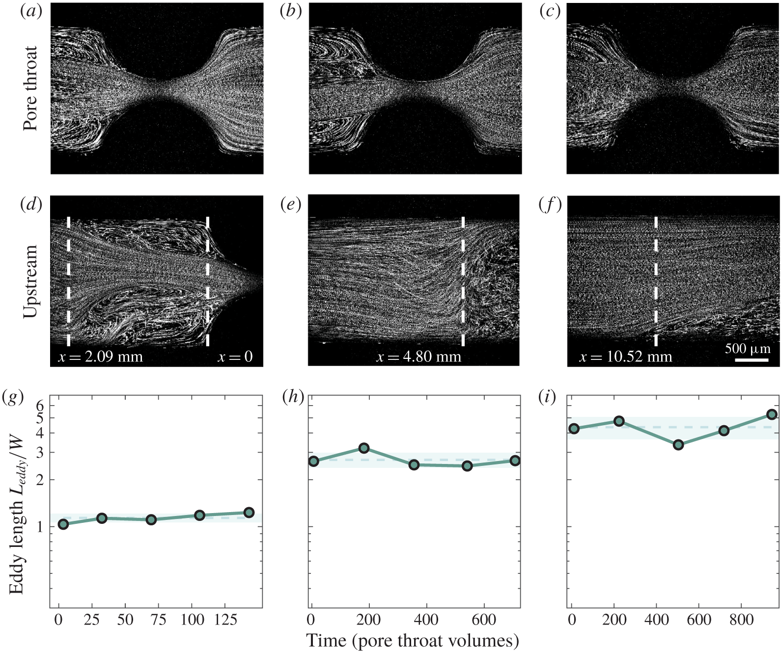
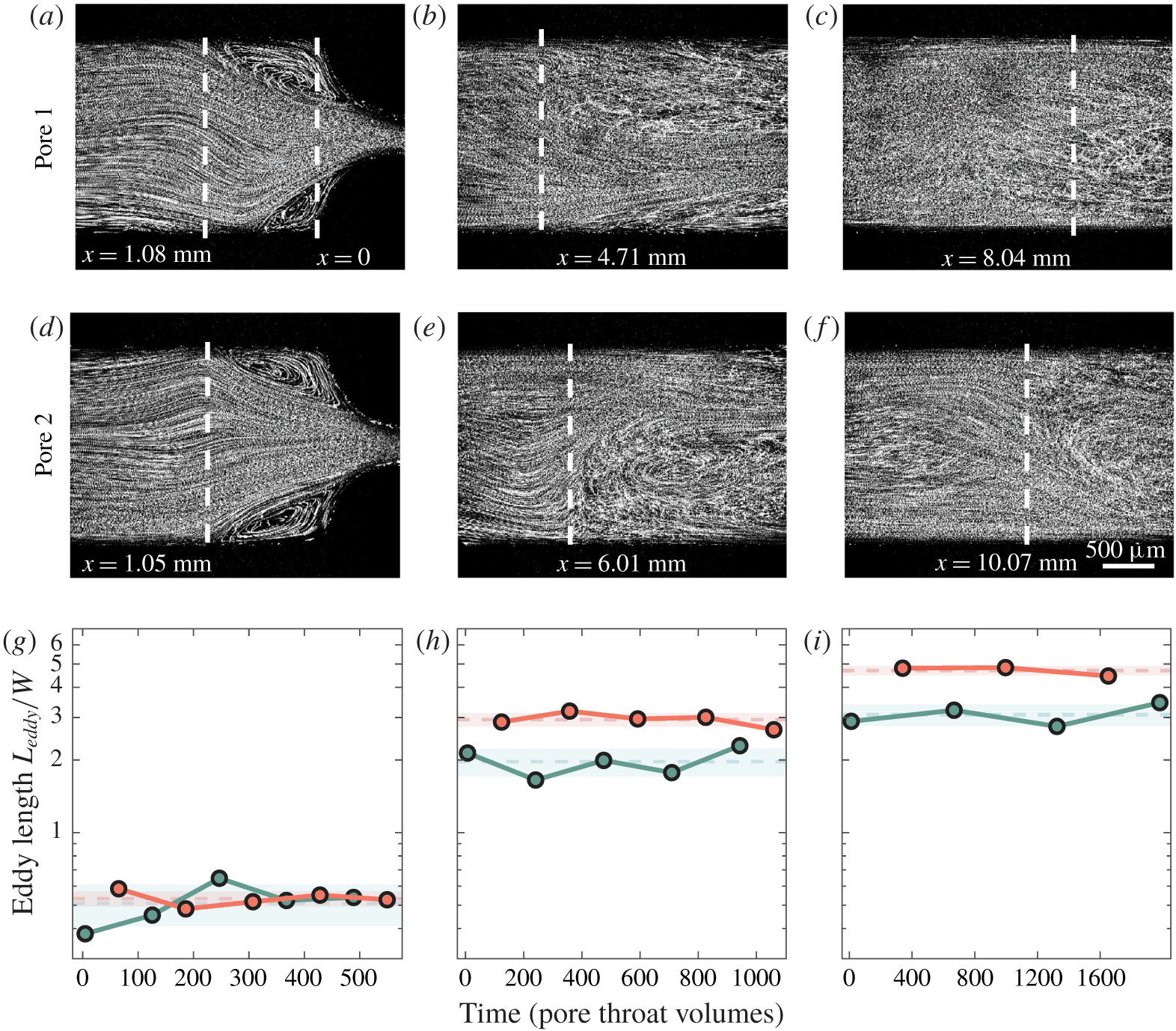
 $M\approx 19$, we observe the onset of a flow instability: a pair of unstable eddies forms against the channel walls upstream of the pore throat, as exemplified in figures 3(a–c) (at the pore throat) and 3(d–f) (upstream) for
 $M=19.4$, 23.9 and 30.5.
Pathline images of polymer solution flow through a straight channel with a single pore throat. Pathline images are averaged over  $10\unicode[STIX]{x1D70F}_{pv}$. Flow rates are expressed via the
 $M$ parameter, which equals 19.4, 23.9 and 30.5 for panels (a), (b) and (c), respectively, corresponding to Weissenberg numbers
 $Wi=5.6$, 6.9 and 8.8. Panels (a–c) show strong recirculating eddies upstream of the pore throat, but no downstream eddies at any flow rate. Panels (d–f) show the leftmost edge of the eddies in front of the pore throat. Dashed lines indicate where the eddy-dominated region begins. Here,
 $x$ indicates the distance in millimetres from the base of the hemi-cylinder. Panels (g–i) show the measured eddy length over time normalized by
 $\unicode[STIX]{x1D70F}_{pv}$. Shaded regions show standard deviation around the temporal mean (dashed lines).

Within each eddy, the fluid recirculates with a speed slower than the mean imposed flow speed in the channel. The fluid pathlines continually fluctuate on long time scales, and also continually cross, indicating that fluctuations in the flow occur on a time scale shorter than the pathline duration of  $10\unicode[STIX]{x1D70F}_{pv}$ (figure 3d–f). These fluctuations are reflected in the motions of the eddy boundaries and lengths, which also fluctuate as the flow progresses. Similarly, while the fluid in the region formed between the eddies does not recirculate, the fluid pathlines also continually fluctuate on long time scales and continually cross, reflecting the presence of rapid fluctuations in the flow throughout. By contrast, the flow is more steady downstream of the pore throat: we do not observe any eddies or marked temporal changes in the flow for all values of
 $M$ tested. This result is consistent with the findings of Qin et al. (Reference Qin, Salipante, Hudson and Arratia2019), who also found highly unstable eddies upstream of a cylinder in a channel, but suppressed fluctuations and no eddies downstream. We therefore focus our subsequent analysis on the upstream region.
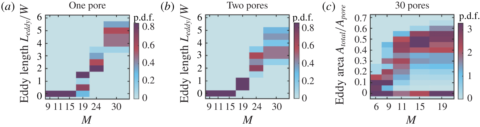
Probability density functions of measured eddy sizes for different values of  $M$, averaged over at least
 $7\unicode[STIX]{x1D70F}_{pv}$ and over two separate replicate experiments, displayed vertically as heatmaps. (a) Probability density functions of
 $L_{eddy}/W$ for a channel with a single pore throat constriction. For each value of
 $M$ there is a single characteristic eddy length that increases monotonically with
 $M$. (b) Probability density functions of
 $L_{eddy}/W$ for a channel with two widely spaced pores
 $l_{s}=16W$ apart. Again, for each value of
 $M$ there is a single characteristic eddy length that increases monotonically with
 $M$. (c) Probability density functions of
 $A_{total}/A_{pore}$ for a porous medium with 30 closely spaced pores
 $l_{s}=W$ apart. Here, the probability density functions for
 $M>9$ are bimodal, showing multiple characteristic eddy areas (one peak at
 $A_{eddy}/A_{pore}\approx 60\,\%$ and one peak at
 $A_{eddy}/A_{pore}\approx 0$). The two branches in the probability density functions indicate a bistability in unstable flow states.

To further characterize this behaviour, we track the eddy length  $L_{eddy}$ over time for each value of
 $M$ tested. We measure
 $L_{eddy}$ from the base of the hemi-cylinders (
 $x=0$ in figure 3d) to the farthest upstream location having a pathline oriented perpendicular to the imposed flow direction (dashed lines in figure 3d–f). Consistent with the visual observations,
 $L_{eddy}$ fluctuates over time in each experiment, as indicated by the shaded regions in figure 3(g–i); however, it fluctuates around a single mean value that increases with
 $M$. We quantify these fluctuations using the coefficient of variation
 $c_{v}$, defined as the ratio between the standard deviation and the mean of the measurements of
 $L_{eddy}$ over time. Taking data from two replicate experiments at these imposed flow rates, we find
 $c_{v}\approx 0.3$, 0.3 and 0.4 for
 $M=19.4$, 23.9 and 30.5, respectively.
We summarize all of our measurements by plotting the probability density (p.d.f.) of time-averaged measured eddy lengths for each value of  $M$ tested. Below the threshold value of
 $M\approx 19$, we do not observe eddies and hence
 $L_{eddy}=0$. By contrast, above this threshold,
 $L_{eddy}>0$ fluctuates about a well-defined mean value, which increases with
 $M$, as shown in figure 4(a). This increase in
 $L_{eddy}$ is similar to previous measurements for isolated constrictions; these studies demonstrate that eddies form when polymers are elongated, and the size of eddies grows as polymers are increasingly elongated (Batchelor Reference Batchelor1971; Boger Reference Boger1987; Mongruel & Cloitre Reference Mongruel and Cloitre1995, Reference Mongruel and Cloitre2003; Rodd et al. Reference Rodd, Cooper-White, Boger and McKinley2007). Our results thus suggest that flow fluctuations arising from unstable flow elongate the individual polymer chains (Sureshkumar, Beris & Handler Reference Sureshkumar, Beris and Handler1997; Balkovsky, Fouxon & Lebedev Reference Balkovsky, Fouxon and Lebedev2000; Chertkov Reference Chertkov2000; Gupta, Sureshkumar & Khomami Reference Gupta, Sureshkumar and Khomami2004; Terrapon et al. Reference Terrapon, Dubief, Moin, Shaqfeh and Lele2004), which then generate unstable upstream eddies to minimize extensional stresses (Batchelor Reference Batchelor1971; Boger Reference Boger1987; Mongruel & Cloitre Reference Mongruel and Cloitre1995, Reference Mongruel and Cloitre2003; Rodd et al. Reference Rodd, Cooper-White, Boger and McKinley2007).
Pathline images of polymer solution flow through a straight channel with two pore throats separated by  $l_{s}=16W$. Pathline images are averaged over
 $10\unicode[STIX]{x1D70F}_{pv}$. Flow rates are expressed via the
 $M$ parameter, which equals 19.4, 23.9 and 30.5 for (a), (b) and (c), respectively, corresponding to
 $Wi=5.6$, 6.9 and 8.8. Panels (a–c) show the leftmost edge of the eddies in front of the first pore throat. Panels (d–f) show the leftmost edge of the eddies in front of the second pore throat. No eddies are observed downstream of either throat. Panels (g–i) show the measured eddy lengths over time normalized by
 $\unicode[STIX]{x1D70F}_{pv}$ for pore 1 (green) and pore 2 (red). Shaded regions show standard deviation around the temporal mean (dashed lines).

3.2 Two widely spaced pore throats
We next investigate two pore throats spaced a distance  $l_{s}=16W$ apart along the flow direction. As we find with an isolated throat, the flow is laminar at low values of
 $M$, while above a similar threshold value of
 $M\approx 19$, we observe the onset of the flow instability. A pair of unstable eddies again forms against the channel walls upstream of each pore throat, as exemplified in figures 5(a–c) (first throat) and 5(d–f) (second throat). Moreover, as with the isolated pore throat, the flow is more steady immediately downstream of each throat, with no observable eddies or temporal changes in the flow for any values of
 $M$ tested.
We again quantify this behaviour by measuring  $L_{eddy}$ over time for each value of
 $M$ tested. For each pore throat,
 $L_{eddy}$ again fluctuates around a single mean value that increases with
 $M$ (figure 5g–i) – similar to the case of an isolated throat. The p.d.f.s of the combined time-averaged measurements of
 $L_{eddy}$ also reflect its increase with
 $M$, as shown in figure 4(b). Intriguingly, however, we observe two key differences from the isolated throat. First, while the mean values of
 $L_{eddy}$ are similar for the two pore throats, eddies upstream of the second throat (red points, figure 5g–i) are slightly larger than eddies upstream of the first throat (green points) for large values of
 $M$. Second, the eddies upstream of the second throat are less unstable – the temporal fluctuations in
 $L_{eddy}$ are notably suppressed for the second pore throat for all
 $M$ above the threshold for unstable flow (compare red to green shaded regions in figure 5g–i). Comparing the coefficients of variation confirms this finding: for the first pair of eddies,
 $c_{v}=0.2\pm 0.1$ while for the second pair,
 $c_{v}=0.10\pm 0.02$, which is significantly smaller (
 $p=0.02$, one-tailed
 $t$-test). Thus, when the spacing between pore throats is reduced, the spatio-temporal characteristics of the flow are altered – presumably because polymer elongation can persist across multiple pores.
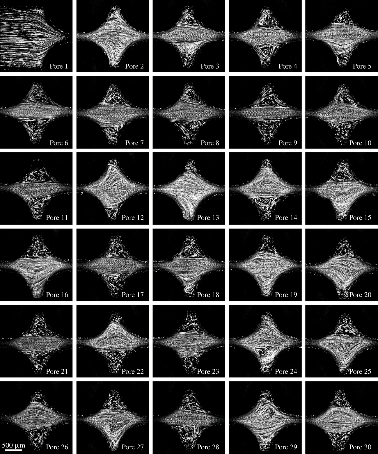
Pathline images of polymer solution flow through a porous medium with 30 pore throats separated by  $l_{s}=W=2~\text{mm}$ at
 $M=11.4$. Images span 2.11 mm across. Pathline images are averaged over
 $10\unicode[STIX]{x1D70F}_{pv}$. Pore 6 exemplifies the eddy-dominated state, with eddies that continually fluctuate both internally and at their boundaries, while pore 2 exemplifies the eddy-free state, with strongly fluctuating pathlines that fill the entire pore body.

3.3 Thirty closely spaced pore throats
To further test the hypothesis that polymer memory impacts flow behaviour, we next investigate flow through a medium with an even smaller spacing between pore throats. Specifically, the flow channel contains 30 pore throats spaced a distance  $l_{s}=W$ apart along the flow direction. In this case, we find that the flow behaviour is strikingly different from the larger
 $l_{s}$ cases described in §§ 3.1 and 3.2.
One key difference is that the threshold for the onset of the flow instability is dramatically lowered. At low imposed flow rates, and thus at low values of  $M$, the flow is laminar: the fluid pathlines do not cross and do not vary over time. In this regime, a pair of small, symmetric, laminar, recirculating eddies forms in the corners of each pore body due to the small spacing between successive pore expansions and constrictions. Above a threshold value of
 $M\approx 9$ – considerably smaller than the threshold
 $M\approx 19$ for the single- and double-throat cases – we observe the onset of unstable flow: the fluid pathlines continually cross and vary over time. Thus, decreasing the spacing between pore throats decreases the threshold value of
 $M$ required for unstable flow, suggesting that polymer memory strongly impacts the flow behaviour.
Even more strikingly, we observe two distinct flow states that can arise in each pore body throughout the medium: an ‘eddy-dominated’ state in which a pair of large unstable eddies forms in the corners of the pore body, and an ‘eddy-free’ state in which strongly fluctuating fluid pathlines fill the entire pore body and eddies do not form. This surprising bistability is illustrated in figure 6, which shows the pathline images taken sequentially from each pore in the medium at  $M=11.4$. Pore 6 exemplifies the eddy-dominated state, with eddies that continually fluctuate both internally and at their boundaries, while pore 2 exemplifies the eddy-free state, with strongly fluctuating pathlines that fill the entire pore body. Though these snapshots are taken at an optical slice in the centre of the channel height, imaging at other heights shows similar flow pathlines, indicating that the spatial structure of the flow does not vary appreciably across the channel height. This observation is in stark contrast to the typical assumption that flow behaviour in a porous medium is determined just by injection conditions and the geometry of the individual pores (Zami-Pierre et al. Reference Zami-Pierre, De Loubens, Quintard and Davit2016). Instead, we find that different pores can exhibit distinct flow characteristics, even when the individual pore geometries and imposed flow rates are all identical.
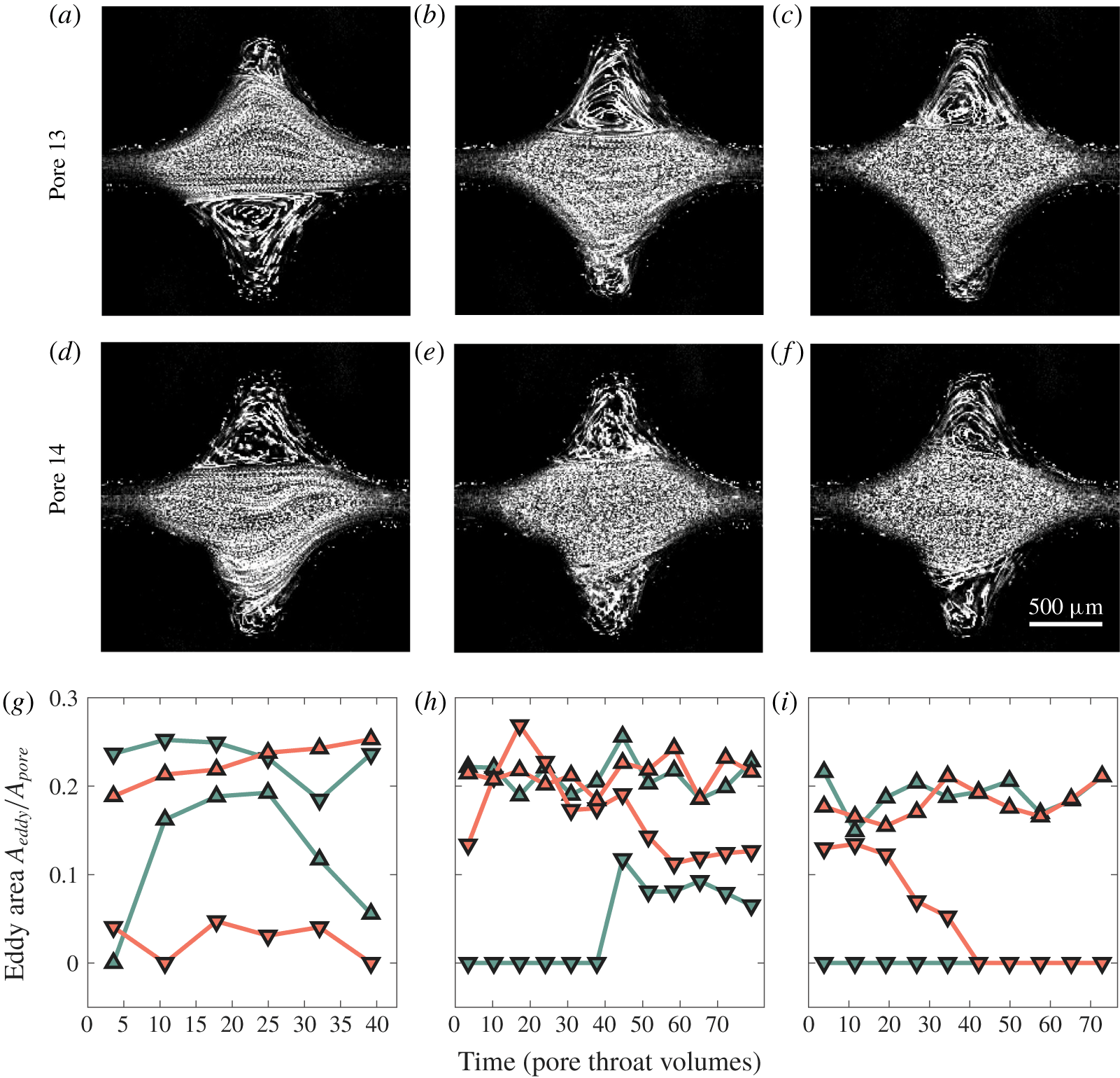
Pathline images of polymer solution flow through pores 13 (a–c) and 14 (d–f) at different flow rates corresponding to  $M=11.4$, 15 and 19.4 (left to right). Pathline images are averaged over
 $10\unicode[STIX]{x1D70F}_{pv}$. Panels (g–i) show the measured eddy areas
 $A_{eddy}/A_{pore}$ over time normalized by
 $\unicode[STIX]{x1D70F}_{pv}$ for pore 13 (green) and pore 14 (red). Upward triangles are for the top region of the pore body, downward triangles are for the bottom region of the pore body.

To quantify this behaviour, we measure the two-dimensional (2-D) area of the individual eddies  $A_{eddy}$ over time for each value of
 $M$ tested. In laminar flow, the eddies occupy only
 ${\approx}5\,\%$ of the total area of a pore, which we define as
 $A_{pore}\equiv Wl_{s}-\unicode[STIX]{x03C0}D_{p}^{2}/4$. By contrast, unstable eddies in the eddy-dominated state have values of
 $A_{eddy}$ that fluctuate strongly in time, and whose mean value can be up to
 ${\approx}30\,\%$ of
 $A_{pore}$, while in the eddy-free state
 $A_{eddy}\approx 0$. Intriguingly, while the two flow states are each unstable, the flow behaviour in each pore body appears to be bistable, as illustrated in figure 7: a pore will persist in a given unstable flow state for a long duration of time before switching, seemingly randomly, to the other flow state. For example, at
 $M=11.4$, the upper eddy in pore 13 and the lower eddy in pore 14 (figure 7g, upward-pointing red triangles and downward-pointing green triangles, respectively) persist in the eddy-dominated state over the entire imaging duration, while the lower eddy in pore 13 persists in the eddy-free state (downward red triangles). However, the upper eddy in pore 14 initially switches from the eddy-free to the eddy-dominated state, in which it persists for
 $15\unicode[STIX]{x1D70F}_{pv}$ before switching back to the eddy-free state (upward green triangles). We observe this flow bistability in all pores of the medium, and at all values of
 $M$ tested; two more examples for
 $M=15$ and 19.4 are shown in figure 7(h–i), respectively.
To further characterize the flow bistability shown in figure 7(g–i), we plot the p.d.f.s of the time-averaged measurements of  $A_{total}$, which describes the total
 $A_{eddy}$ measured in each pore combined for all 30 pores in the medium. Below
 $M\approx 9$,
 $A_{total}\approx 10\,\%$ of
 $A_{pore}$, and eddies do not change in time; by contrast, above the onset of the flow instability at
 $M\approx 9$, the p.d.f.s become bimodal, reflecting the bistability in flow behaviour (figure 4c). The eddy-dominated state is represented by the upper branch of the p.d.f.s, in which
 $A_{total}$ increases with
 $M$, eventually plateauing at
 ${\approx}60\,\%$ of
 $A_{pore}$ at the highest values of
 $M$ tested. The eddy-free state is represented by the lower branch of the p.d.f.s, in which
 $A_{total}\approx 0$ over all
 $M$. This bistability does not arise in porous media with wider pore spacings: the lower branch of the p.d.f.s does not appear in figure 4(a,b). Thus, when the spacing between pore throats is reduced from
 $l_{s}=16W$ to
 $l_{s}=W$ – and thus, elongation of individual polymers is more likely to persist across multiple pores – the flow abruptly becomes bistable, exhibiting two coexisting unstable flow states. Indeed, previous work has theorized that unstable flow may bifurcate into two coexisting flow states (Avgousti & Beris Reference Avgousti and Beris1993; Sureshkumar, Beris & Avgousti Reference Sureshkumar, Beris and Avgousti1994; Varshney & Steinberg Reference Varshney and Steinberg2017); to our knowledge, our work is the first experimental confirmation of this prediction.
3.3.1 Bistability and polymer conformations in flow
How does this unusual flow bistability arise? Previous measurements of polymer conformations indicate that differing fractions of coiled and elongated chains coexist in extensional and unstable flows depending on the imposed flow conditions (Schroeder et al. Reference Schroeder, Babcock, Shaqfeh and Chu2003; Gerashchenko, Chevallard & Steinberg Reference Gerashchenko, Chevallard and Steinberg2005; François et al. Reference François, Amarouchene, Lounis and Kellay2009). Furthermore, simulations indicate that polymers having different elongation can have dramatically differing pore-scale flow behaviours (Pilitsis & Beris Reference Pilitsis and Beris1989, Reference Pilitsis and Beris1991). Thus, we hypothesize that flow bistability arises from the interplay between flow-induced polymer elongation, which promotes eddy formation, and relaxation of polymers as they are advected between pores, which enables the eddy-free state to form.
We first consider a pore in the eddy-dominated state. Polymers entering the pore are likely in an elongated conformation due to the combined influence of unstable flow fluctuations and extension by flow converging into the upstream pore throat. Indeed, previous work has demonstrated that eddies form upstream of a constriction when polymers are elongated (Batchelor Reference Batchelor1971; Boger Reference Boger1987; Mongruel & Cloitre Reference Mongruel and Cloitre1995, Reference Mongruel and Cloitre2003; Rodd et al. Reference Rodd, Cooper-White, Boger and McKinley2007). Eddy formation minimizes extensional stresses in the centre of the pore: the net flow through the pore body occurs in a nearly straight channel spanning one pore throat to the next, as can be seen in the example of pore 6 in figure 6. For simplicity, we consider the limit of large  $M$, in which eddies completely fill the corners of the pore body. With the exception of unstable fluctuations, the flow velocities in this channel are then aligned along the flow direction with speed
 ${\sim}U_{t}\equiv Q/A_{t}\sim 1~\text{mm}~\text{s}^{-1}$, and therefore the extensional component of the flow in the channel is minimal. The elongated polymers thus continue to relax as they are advected through this channel, reaching their equilibrium coiled conformation after a duration
 ${\sim}\unicode[STIX]{x1D706}_{rel}$, the chain relaxation time. We compare this time scale to the residence time required for the polymers to transit across the pore body from the upstream throat to the downstream throat,
 ${\sim}l_{s}/U_{t}$, yielding an advective Deborah number
 $De_{adv}\equiv \unicode[STIX]{x1D706}_{rel}U_{t}/l_{s}$. When
 $l_{s}$ is small and
 $De_{adv}\gtrsim 1$, chains are still elongated as they enter the next pore body, thereby promoting eddy formation in the current pore and the downstream pore as well. For our experiments in the unstable regime with
 $l_{s}=W$,
 $De_{adv}$ ranges from
 ${\sim}0.5$ to
 $3$ using
 $\unicode[STIX]{x1D706}_{rel}\sim \unicode[STIX]{x1D706}\approx 1$ s; this estimate likely underestimates
 $De_{adv}$, since
 $\unicode[STIX]{x1D706}_{rel}$ is known to increase considerably in extensional flow (Clasen et al. Reference Clasen, Plog, Kulicke, Owens, Macosko, Scriven, Verani and McKinley2006). Thus, we expect the eddy-dominated state to persist in the pore body over time before random flow fluctuations cause it to switch to the eddy-free state, consistent with our measurements shown in figure 7(g–i). We also expect the eddy-dominated state to be correlated between neighbouring pores.
We next consider the formation of the eddy-free state. As polymers pass through eddy-dominated pores, they gradually relax to the coiled conformation. When a sufficient fraction of coiled polymers are at the entrance to a pore, there will be no driving force for eddy formation. The pore will thus be in the eddy-free state. The fluid streamlines then diverge from the upstream pore throat, creating a compressional flow that further promotes the coiled conformation. As the polymers continue to traverse the pore body, they remain coiled until they encounter the converging flow into the downstream pore throat. This extensional flow partially elongates the chains, which requires a time scale  ${\sim}\unicode[STIX]{x1D706}_{ret}$. We again compare this time scale to the residence time required for the polymers to transit from the beginning of the converging region to the downstream throat, in this case
 ${\sim}H(WD_{p}/2-\unicode[STIX]{x03C0}D_{p}^{2}/8)/Q$. This comparison yields another advective Deborah number
 $De_{adv}^{\prime }\equiv \unicode[STIX]{x1D706}_{ret}Q/[H(WD_{p}/2-\unicode[STIX]{x03C0}D_{p}^{2}/8)]$. When
 $De_{adv}^{\prime }\gtrsim 1$, chains are not elongated as they enter the next pore body, thereby promoting the eddy-free state in the current pore and the downstream pore as well. For our experiments in the unstable regime,
 $De_{adv}^{\prime }$ ranges from
 ${\approx}0.7$ to 5 using
 $\unicode[STIX]{x1D706}_{ret}\sim \unicode[STIX]{x1D706}\approx 1$ s, although these values again likely underestimate
 $De_{adv}^{\prime }$. Thus, similar to the eddy-dominated state, we expect the eddy-free state to persist in the pore body over time before random flow fluctuations cause it to switch to the eddy-dominated state, consistent with our measurements shown in figure 7(g–i). Moreover, we again expect the eddy-free state to be correlated between neighbouring pores.
3.3.2 Temporal and spatial characteristics of the flow
The hypothesis presented in § 3.3.1 makes two testable predictions: first, that the two different unstable flow states each persist over long times before randomly switching, and second, that the flow states between neighbouring pores  $n$ and
 $n+1$ are correlated. We test these predictions by investigating the temporal and spatial characteristics of the pore-scale flow. Specifically, we simultaneously image two neighbouring pores within the medium, pores
 $n=21$ and
 $n+1=22$, at
 $M=15$ and monitor the flow states for
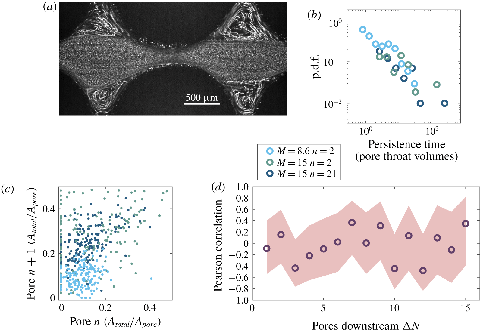
 $2500\unicode[STIX]{x1D70F}_{pv}$. Figure 8(a) shows a snapshot of the flow pathlines imaged simultaneously and averaged over
 $10\unicode[STIX]{x1D70F}_{pv}$ at an instance when both pores are in the eddy-dominated state.
(a) Simultaneous pathline imaging of pores 21 and 22 averaged over  $10\unicode[STIX]{x1D70F}_{pv}$ for
 $M=15.0$. Both pores are in the eddy-dominated state. (b) Probability density function of times between discrete switching events, representing the duration over which a given flow state persists in pores
 $n$ or
 $n+1$, for pores imaged over at least
 $400\unicode[STIX]{x1D70F}_{pv}$. For panels (b) and (c), light blue shows
 $M=8.6$ for
 $n=2$, teal blue shows
 $M=15$ for
 $n=2$, and navy blue shows
 $M=15$ for
 $n=21$. The data are broadly distributed with long tails. (c) Instantaneous eddy areas of pores
 $n$ and pore
 $n+1$ are positively correlated, indicating that flow states are correlated between neighbouring pores. (d) Pearson correlation coefficients between pores separated by a length
 $l_{s}\unicode[STIX]{x0394}N$ and imaged sequentially a time
 $80\unicode[STIX]{x1D70F}_{pv}\unicode[STIX]{x0394}N$ apart for
 $M=15.0$. The flow state of each pore is averaged over
 $80\unicode[STIX]{x1D70F}_{pv}$. Thus, this analysis only quantifies any possible long-time correlations that persist over time scales larger than
 $80\unicode[STIX]{x1D70F}_{pv}\unicode[STIX]{x0394}N$. Light red shaded region indicates 99 % confidence interval for estimated correlation coefficient given the sampling size.

The data in figure 7(g–i) support the first prediction that the two distinct flow states persist over long times. To further test this prediction, we measure the distribution of durations over which each flow state persists in a given pore before switching to the other state; we define a switching event as the instant when the total eddy area  $A_{total}$ in a given pore crosses a threshold value of
 $0.05~A_{pore}$. This threshold is motivated by the clear separation between the eddy-dominated and eddy-free states indicated by the probability density function in figure 4(c). In agreement with our expectation, we find a broad distribution of long flow persistence times with no characteristic persistence time, as shown by the navy blue points in figure 8(b) – confirming our first prediction. Indeed, theoretical predictions for two-state systems that have self-stabilizing states – similar to the eddy-dominated and eddy-free states described here – also predict broad distributions of state persistence times (Ali, Wingreen & Mukhopadhyay Reference Ali, Wingreen and Mukhopadhyay2018).
The image in figure 8(a) supports the second prediction that the flow states in neighbouring pores are correlated. To further test this prediction, we measure the instantaneous total eddy areas  $A_{total,n}$ and
 $A_{total,n+1}$ in pores
 $n=21$ and
 $n+1=22$ by imaging both pores simultaneously over several thousand
 $\unicode[STIX]{x1D70F}_{pv}$. To visualize the pathlines of the individual tracer particles, we average successive frames for
 $10\unicode[STIX]{x1D70F}_{pv}$; this procedure enables us to determine the presence or absence of recirculating eddies in the pore bodies and provides a way to directly measure the eddy areas by tracking the eddy boundaries, as exemplified in figure 8(a). We thereby compute the total eddy area
 $A_{total}$ in each pore body of area
 $A_{pore}$. Over the course of this experiment, the pore bodies exhibit the full range of flow behaviours: we measure the full range of possible total eddy sizes for each pore body, ranging from
 $A_{total}=0$ to the maximal value
 $A_{total}\approx 0.5A_{pore}$. Then, to quantify the correlation in flow state between pores
 $n$ and
 $n+1$, we plot the total eddy areas simultaneously measured for both pores at different times,
 $A_{total,n}$ and
 $A_{total,n+1}$, respectively. These measurements show a positive correlation between the instantaneous flow states of neighbouring pores
 $n=21$ and
 $n+1=22$ over the imaging duration, as shown by the navy blue points in figure 8(c). We quantify this correlation using the Pearson correlation coefficient
 $\unicode[STIX]{x1D70C}_{n,n+1}\equiv \text{cov}(A_{total,n},A_{total,n+1})/[\unicode[STIX]{x1D70E}(A_{total,n})\unicode[STIX]{x1D70E}(A_{total,n+1})]$, where
 $\text{cov}$ is the covariance and
 $\unicode[STIX]{x1D70E}$ is the standard deviation of the instantaneous measurements of
 $A_{total,n}$ and
 $A_{total,n+1}$ over the different times. We find
 $\unicode[STIX]{x1D70C}_{21,22}=0.55>0$, confirming a positive correlation between the eddy sizes in the neighbouring pores 21 and 22 that is statistically significant (
 $p<0.001$, two-tailed
 $t$-test). Thus, the unstable flow states in neighbouring pores are correlated with each other, confirming our second prediction.
To further test how this behaviour varies spatially and with  $M$, we repeat these measurements near the inlet at pores
 $n=2$ and
 $n+1=3$ at two different flow rates corresponding to
 $M=15$ and
 $M=8.6$. We expect that decreasing the flow rate will decrease the advective Deborah numbers
 $De_{adv}$ and
 $De_{adv}^{\prime }$; thus we expect that at lower flow rates, unstable flow states will still be broadly distributed, but will persist over shorter time scales. Our data confirm this expectation: we find that at the lower flow rate, flow states persist for slightly shorter times, as indicated by the light blue points (
 $M=8.6$,
 $n=2$) compared to the teal blue points (
 $M=15$,
 $n=2$) shown in figure 8(b). The unstable flow states in neighbouring pores remain positively correlated with each other in both cases, as shown by the light blue and teal blue points in figure 8(c); the corresponding Pearson correlation coefficients are
 $\unicode[STIX]{x1D70C}_{2,3}=0.25>0$ and
 $\unicode[STIX]{x1D70C}_{2,3}=0.21>0$, respectively, confirming a positive correlation that is statistically significant (
 $p<0.001$, two-tailed
 $t$-test). This positive correlation likely reflects the fact that, even at the lower flow rate with
 $M=8.6$, both
 $De_{adv}\approx 0.5$ and
 $De_{adv}^{\prime }\approx 0.7$ are close to one, and thus, flow states are still likely to be correlated between neighbours. Intriguingly, while the correlation coefficient does not depend strongly on
 $M$ for this range of flow rates, it does increase with position along the flow direction: for the same
 $M=15$,
 $\unicode[STIX]{x1D70C}_{2,3}=0.21$ while
 $\unicode[STIX]{x1D70C}_{21,22}=0.55$, suggesting that flow states in neighbouring pores become increasingly correlated downstream. Further exploring this spatial dependence of correlations in unstable flow state will be a useful direction for future work.
While neighbouring pores exhibit correlated flow states on short time scales, imaging of flow through the entire medium (figure 6) suggests that these correlations are not sufficient to produce long-range correlations in the flow over long times. Indeed, as quantified by the measurements in figure 8(b), we do not expect correlations to persist, even for neighbouring pores, when flow state is averaged over sufficiently long time scales. To test this expectation, we sequentially image pores  $n=2$ through
 $n=30$ for
 $80\unicode[STIX]{x1D70F}_{pv}$ each. We use these data to compute the time-averaged eddy area in each pore,
 $\bar{A}_{total,2}$ through
 $\bar{A}_{total,30}$, where each value of
 $\bar{A}_{total}$ is averaged over
 $80\unicode[STIX]{x1D70F}_{pv}$. We then quantify any possible correlations between these 29 measurements of the time-averaged eddy areas using the correlation coefficient
 $\unicode[STIX]{x1D70C}_{n,n+\unicode[STIX]{x0394}N}\equiv \text{cov}(\bar{A}_{total,n},\bar{A}_{total,n+\unicode[STIX]{x0394}N})/[\unicode[STIX]{x1D70E}(\bar{A}_{total,n})\unicode[STIX]{x1D70E}(\bar{A}_{total,n+\unicode[STIX]{x0394}N})]$, which in this case quantifies correlations between the measured
 $\bar{A}_{total}$ for all pores
 $n$ and
 $n+\unicode[STIX]{x0394}N$ that are thus separated by a length
 $l_{s}\unicode[STIX]{x0394}N$; here, cov is the covariance and
 $\unicode[STIX]{x1D70E}$ is the standard deviation of the time-averaged measurements of
 $\bar{A}_{total,n}$ and
 $\bar{A}_{total,n+\unicode[STIX]{x0394}N}$, for a given value of
 $\unicode[STIX]{x0394}N$ ranging from 1 to 15, over the different values of
 $n$. In this analysis, instead of tracking the instantaneous correlation for many different time points as before, we track a time-averaged correlation for many different pairs of pores. Thus, this correlation analysis does not capture any possible flow correlations
 $\unicode[STIX]{x0394}N$ pores apart those that arise on time scales shorter than
 $80\unicode[STIX]{x1D70F}_{pv}\unicode[STIX]{x0394}N$: it only quantifies any possible long-time correlations that persist over time scales larger than
 $80\unicode[STIX]{x1D70F}_{pv}\unicode[STIX]{x0394}N$. Consistent with our expectation, we do not find long-time correlations in flow state, even between nearest neighbours: the correlation coefficient does not statistically deviate from zero for any values of
 $\unicode[STIX]{x0394}N$ throughout the medium, as shown in figure 8(d). Thus, while unstable flow states are correlated over short times across neighbouring pores, these correlations do not persist over long time scales – presumably due to the influence of random fluctuations in the flow, which likely promote switching between flow states. Our data do not preclude the possibility that longer-range correlations may arise at shorter time scales, or that correlations in flow state can evolve spatially throughout the medium; indeed, previous work has indicated that velocity correlations can coherently propagate through other experimental geometries (Qin et al. Reference Qin, Salipante, Hudson and Arratia2019). Investigating whether the flow correlations described in figure 8(a–c) can persist over broader spatial and temporal ranges will be a useful direction for future work.
4 Conclusions
Our work describes the first experimental observations of bistability in the flow of an elastic polymer solution through porous media, confirming previous theoretical predictions (Avgousti & Beris Reference Avgousti and Beris1993; Sureshkumar et al. Reference Sureshkumar, Beris and Avgousti1994; Varshney & Steinberg Reference Varshney and Steinberg2017). We find that when the spacing between pores is sufficiently small, and when the imposed flow rate is sufficiently large, the flow stochastically switches between two distinct unstable flow states. In the eddy-dominated state, a pair of large unstable eddies forms in the corners of a pore body, while in the eddy-free state, strongly fluctuating fluid pathlines fill the entire pore body and eddies do not form. Our results thus indicate that in a porous medium the pore-scale flow behaviour may not be determined just by injection conditions – as quantified by the Weissenberg number  $Wi$ or the
 $M$ parameter (McKinley et al. Reference McKinley, Pakdel and Öztekin1996; Pakdel & McKinley Reference Pakdel and McKinley1996) – and the geometry of the individual pores, as is often assumed.
Our model 1-D geometry does not incorporate pore size disorder, tortuosity and connectivity for simplicity; it instead provides a way to isolate and systematically probe the role of pore spacing on flow behaviour. Incorporating these additional complexities in the medium geometry, and extending our findings to 2-D and 3-D media in which transverse interactions between pores may also play a role (Talwar & Khomami Reference Talwar and Khomami1995; Khomami & Moreno Reference Khomami and Moreno1997; Arora et al. Reference Arora, Sureshkumar and Khomami2002; Sadanandan & Sureshkumar Reference Sadanandan and Sureshkumar2004; Vázquez-Quesada & Ellero Reference Vázquez-Quesada and Ellero2012; Howe, Clarke & Giernalczyk Reference Howe, Clarke and Giernalczyk2015; Clarke et al. Reference Clarke, Howe, Mitchell, Staniland and Hawkes2016; De et al. Reference De, Kuipers, Peters and Padding2017a,Reference De, Kuipers, Peters and Paddingb,Reference De, Kuipers, Peters and Paddingc,Reference De, van der Schaaf, Deen, Kuipers, Peters and Paddingd, Reference De, Koesen, Maitri, Golombok, Padding and van Santvoort2018a,Reference De, Krishnan, van der Schaaf, Kuipers, Peters and Paddingb; Kawale et al. Reference Kawale, Marques, Zitha, Kreutzer, Rossen and Boukany2017b,Reference Kawale, Bouwman, Sachdev, Zitha, Kreutzer, Rossen and Boukanya; Walkama, Waisbord & Guasto Reference Walkama, Waisbord and Guasto2019), will be an important direction for future studies. Moreover, because pressure drop measurements are often used to characterize flow through porous media (Sandiford et al. Reference Sandiford1964; Chauveteau & Moan Reference Chauveteau and Moan1981; Durst et al. Reference Durst, Haas and Kaczmar1981; Chauveteau et al. Reference Chauveteau, Moan and Magueur1984; Pitts et al. Reference Pitts, Campbell, Surkalo and Wyatt1995; Wang et al. Reference Wang, Wang and Xia2011a; Vermolen et al. Reference Vermolen, Van Haasterecht and Masalmeh2014; Wei et al. Reference Wei, Romero-Zerón and Rodrigue2014), exploring the connection between unstable flow states and the macroscopic pressure drop across the medium will also be an important extension of our work.
We hypothesize that the flow bistability arises from the interplay between flow-induced polymer elongation, which promotes eddy formation, and relaxation of polymers as they are advected between pores, which enables the eddy-free state to form. Consistent with this idea, we find that the eddy sizes increase with the imposed flow rate. Additionally, we find that a flow state in a given pore persists over long time scales before switching to the other flow state, presumably due to random flow fluctuations. Flow state is also strongly correlated between neighbouring pores at short time scales; however, these correlations are not sufficient to produce correlations in the flow through the entire medium over long times. Elucidating the factors that determine the length and time scales over which flow correlations persist will be an interesting direction for future work.
While our experiments probe the case of dilute polymer solutions – in which polymer overlap likely does not influence flow behaviour – flow behaviour is known to change considerably at higher concentrations due to the increased propensity of polymer chains to overlap (Kawale et al. Reference Kawale, Bouwman, Sachdev, Zitha, Kreutzer, Rossen and Boukany2017a,Reference Kawale, Marques, Zitha, Kreutzer, Rossen and Boukanyb). We therefore expect that in more concentrated solutions, overlap of polymer chains will increase the relaxation and retardation times  $\unicode[STIX]{x1D706}_{rel}$ and
 $\unicode[STIX]{x1D706}_{ret}$, leading to larger values of the advective Deborah numbers
 $De_{adv}$ and
 $De_{adv}^{\prime }$. Thus, we expect that more concentrated polymer solutions will have correlated flow states that span more pores and that persist over longer time scales.
The different spatial and temporal characteristics of the two flow states described here could impact fluid mixing and the displacement of trapped immiscible fluids from the pore space in a variety of ways (Babayekhorasani et al. Reference Babayekhorasani, Dunstan, Krishnamoorti and Conrad2016; Aramideh, Vlachos & Ardekani Reference Aramideh, Vlachos and Ardekani2019). Thus, a deeper understanding of these flow behaviours could provide guidance to applications that require specific mixing or fluid displacement behaviours. Examples include oil recovery and groundwater remediation, in which the viscous forces exerted by the polymer solution could displace a trapped fluid from the pores, or unstable mixing due to the fluid instability could improve the transport of oxidants and surfactants to the fluid interface. Such flow behaviours could also be harnessed in other emerging applications such as controlling mixing and flow in lab-on-a-chip devices, filtration and extrusion of polymeric resins during 3-D printing.
Acknowledgements
It is a pleasure to acknowledge G. H. McKinley, P. D. Olmsted, A. Z. Panagiotopoulos, R. K. Prud’homme, B. Qin and H. A. Stone for stimulating discussions, and the Stone Lab for access to the SLA printer and the rheometer. Acknowledgement is made to the Donors of the American Chemical Society Petroleum Research Fund for partial support of this research (PRF# no. 59026-DNI9). This material is also based upon work supported by the National Science Foundation Graduate Research Fellowship Program (to C.A.B.) under grant no. DGE-1656466. Any opinions, findings and conclusions or recommendations expressed in this material are those of the authors and do not necessarily reflect the views of the National Science Foundation. C.A.B. was also supported in part by the Mary and Randall Hack Graduate Award of the Princeton Environmental Institute. A.S. was supported in part by the Lidow Thesis Fund at Princeton University and the Dede T. Bartlett P03 Fund for Student Research through the Andlinger Center for Energy and the Environment.
Declaration of interests
The authors report no conflict of interest.
Appendix
The channel dimensions and polymer concentration used in our experiments enable us to isolate the influence of polymer elongation and relaxation between pores, with a minimal influence of polymer surface adsorption, flow-induced chain migration, wall slip, and shear banding, as quantitatively assessed below.
The first effect – polymer adsorption to the solid surfaces and eventual blockage of pore throats – has been documented for media with small pores (Zaitoun et al. Reference Zaitoun and Kohler1988; Zitha, Chauveteau & Zaitoun Reference Zitha, Chauveteau and Zaitoun1995; Zaitoun et al. Reference Zaitoun, Bertin and Lasseux1998; Obey & Griffiths Reference Obey, Griffiths, Goddard and Gruber1999; Zitha, Chauveteau & Léger Reference Zitha, Chauveteau and Léger2001). However, this effect typically influences flow behaviour in media having pore throats much smaller than those explored in our work: the steady state thickness of adsorbed polymers is of the order of polymer molecular dimensions, and for the HPAM polymer used in our experiments, this thickness is  ${\sim}100~\text{nm}$ (Grattoni et al. Reference Grattoni, Luckham, Jing, Norman and Zimmerman2004). Since the thickness of this adsorbed layer is over three orders of magnitude smaller than the smallest channel dimension
 $L_{c}=400~\unicode[STIX]{x03BC}\text{m}$ in our experiments, we do not expect this adsorption layer to appreciably impact the flow. Furthermore, pore blockage is typically exacerbated by the bridging of elongated polymers across the pore throats (Zitha et al. Reference Zitha, Chauveteau and Léger2001); however, the fully elongated contour length of the HPAM polymer is
 $NL_{mon}\approx$
 $40~\unicode[STIX]{x03BC}\text{m}$, where
 $N$ is the degree of polymerization and
 $L_{mon}$ is the monomer Kuhn length. Since this fully elongated contour length is an order of magnitude smaller than the smallest channel dimension
 $L_{c}$, we again do not expect polymer blockage of the pore throats to play a considerable role in our experiments.
Similarly, while flow-induced chain migration and wall slip frequently arise in confined flows of polymer solutions, they give rise to polymer concentration inhomogeneities over length scales  ${\sim}0.1$ to
 $10~\unicode[STIX]{x03BC}\text{m}$ (Kekre, Butler & Ladd Reference Kekre, Butler and Ladd2010), one to three orders of magnitude smaller than
 $L_{c}$. We estimate this length scale by balancing the influence of chain diffusion with elastic normal stresses (Ma & Graham Reference Ma and Graham2005):
 $L_{d}=(9\sqrt{\unicode[STIX]{x03C0}}/128)((N_{1}-N_{2})/nk_{B}T)h^{\ast }R_{g}$, where
 $n$ is the polymer number density in the bulk solution,
 $k_{B}T$ is thermal energy, and
 $R_{g}$ is the polymer radius of gyration. To determine an upper bound for
 $L_{d}$, we take the value of the first normal stress difference
 $N_{1}$ at the maximal shear rate using our shear rheology measurements, and take the second normal stress difference
 $N_{2}$ to be zero. The parameter
 $h^{\ast }=(\unicode[STIX]{x1D701}/\unicode[STIX]{x1D702}_{s})\sqrt{H/36\unicode[STIX]{x03C0}^{3}k_{B}T}=0.07$ quantifies hydrodynamic interactions, where
 $\unicode[STIX]{x1D702}_{s}$ is the shear viscosity of the background solvent,
 $H\approx k_{B}T/2R_{g}^{2}$ is a characteristic polymer spring constant,
 $\unicode[STIX]{x1D701}\approx 4H\unicode[STIX]{x1D706}$ is the monomer hydrodynamic friction coefficient and
 $\unicode[STIX]{x1D706}$ is the polymer relaxation time estimated using shear rheology as described in § 2. Using these values, we obtain
 $L_{d}\approx 20R_{g}=$
 $4~\unicode[STIX]{x03BC}\text{m}$ – in reasonable agreement with measurements that indicate
 $L_{d}\approx NL_{mon}/3\approx 14~\unicode[STIX]{x03BC}\text{m}$ (Fang, Hu & Larson Reference Fang, Hu and Larson2005). These estimated values are one to two orders of magnitude smaller than
 $L_{c}$; thus, we do not expect flow-induced migration to appreciably impact the flow.
Polymer wall slip can play a key role when the flow channel has dimensions approaching molecular dimensions, and for concentrated polymer solutions with a high viscosity ratio  $\unicode[STIX]{x1D6FD}\equiv \unicode[STIX]{x1D702}_{0}/\unicode[STIX]{x1D702}_{s}$, where
 $\unicode[STIX]{x1D702}_{0}$ is the maximal solution shear viscosity and
 $\unicode[STIX]{x1D702}_{s}$ is the shear viscosity of the background solvent. However, in our experiments,
 $L_{c}$ is three orders of magnitude larger than
 $R_{g}$, and our polymer solution is dilute, with
 $\unicode[STIX]{x1D6FD}=1.7$ close to one. Indeed, an upper bound for the length scale over which wall slip occurs
 $L_{s}$ can be estimated (Wang, Ravindranath & Boukany Reference Wang, Ravindranath and Boukany2011b) as
 $L_{s}\leqslant \unicode[STIX]{x1D6FD}R_{g}=330~\text{nm}$. This value is over three orders of magnitude smaller than
 $L_{c}$; thus, we do not expect that wall slip appreciably impacts the flow. Further, we can use this length scale to estimate an upper bound for the wall slip speed
 $U_{s}$ using the wall shear rate
 $\dot{\unicode[STIX]{x1D6FE}}$ in the pore throat at the highest flow rate tested in our experiments; we calculate
 $U_{s}\leqslant L_{s}\dot{\unicode[STIX]{x1D6FE}}\approx 7~\unicode[STIX]{x03BC}\text{m}~\text{s}^{-}1$, over two orders of magnitude smaller than the characteristic flow speeds explored in our experiments. This estimate again suggests that wall slip does not appreciably impact the flow.
Shear banding of polymers often arises during the flow of concentrated polymer solutions. However, our experiments probe the case of dilute polymer solutions, in which polymer overlap likely does not influence flow behaviour and in which shear banding is not expected to occur (Wang et al. Reference Wang, Ravindranath and Boukany2011b). This expectation is further supported by our shear rheology measurements: over the experimental range of shear rates, our measurements of rate-controlled shear rheology indicate that the shear stress varies approximately linearly with shear rate, with a shear thinning exponent  ${\approx}0.92$; by contrast, shear banding typically occurs for solutions in which the shear stress varies non-monotonically with imposed shear rate (Fielding Reference Fielding2007; Olmsted Reference Olmsted2008). We therefore do not expect that shear banding plays an appreciable role in our experiments.