DYNAMIC HYPERSEQUENTS FOR PUBLIC ANNOUNCEMENT LOGIC

CLARA LEROUVILLOIS; FRANCESCA POGGIOLESI

doi:10.1017/S175502032610121X

DYNAMIC HYPERSEQUENTS FOR PUBLIC ANNOUNCEMENT LOGIC

Part of: General logic Proof theory and constructive mathematics

Published online by Cambridge University Press: 25 June 2026

CLARA LEROUVILLOIS

and

FRANCESCA POGGIOLESI

Show author details

CLARA LEROUVILLOIS*: Affiliation:
TOULOUSE INSTITUTE OF COMPUTER SCIENCE RESEARCH UNIVERSITY OF TOULOUSE TOULOUSE FRANCE UNIVERSITÉ PARIS 1 PANTHÉON SORBONNE
FRANCESCA POGGIOLESI: Affiliation:
CNRS IHPST UNIVERSITÉ PARIS 1 PANTHÉON SORBONNE PARIS FRANCE E-mail: poggiolesi@gmail.com
*: E-mail: clara.lerouvillois@irit.fr

Article contents

Abstract
Introduction
Public announcement logic
Dynamic hypersequents for PAL
Admissibility of the structural rules and invertibility of the logical rules
Soundness and completeness
Cut admissibility
Conclusion and future work
Footnotes
References

Rights & Permissions

Abstract

Dynamic epistemic logic extends classical epistemic logic by modeling not only static knowledge but also its evolution through information updates. Among its various systems, public announcement logic (PAL) provides one of the simplest and most studied frameworks for representing epistemic change (see [6]). While the semantics of PAL is well understood as transformation of Kripke models, the existing proof theory might fail to fully capture this dynamism at the syntactic level. In this paper we propose a step toward addressing this gap. In particular, building on the hypersequent calculus for S5 introduced in [15], we extend it with a mechanism that models the transition between epistemic models induced by public announcements. We call these structures dynamic hypersequents (DHSs). Using DHSs, we construct a calculus for PAL and show that it enjoys several desirable properties: admissibility of all structural rules (including contraction), invertibility of logical rules, as well as syntactic cut-elimination.

Keywords

public announcement logic proof theory hypersequents cut-elimination

MSC classification

Primary: 03B42: Logics of knowledge and belief (including belief change) 03B45: Modal logic (including the logic of norms) 03F03: Proof theory, general

Information

Type: Research Article
Information: The Review of Symbolic Logic , Volume 19 , Issue 3 , September 2026 , pp. 491 - 518

DOI: https://doi.org/10.1017/S175502032610121X [Opens in a new window]
Creative Commons: This is an Open Access article, distributed under the terms of the Creative Commons Attribution licence (https://creativecommons.org/licenses/by/4.0/), which permits unrestricted re-use, distribution, and reproduction in any medium, provided the original work is properly cited.
Copyright: © The Author(s), 2026. Published by Cambridge University Press on behalf of The Association for Symbolic Logic

1 Introduction

Dynamic epistemic logic (DEL) [Reference Baltag, Moss and Solecki5, Reference van Ditmarsch, Hoek, Kooi and van Der6] is a branch of logic that emerged in the late 1980s. It extends classical epistemic logic by modeling not only static states of knowledge but also the processes by which knowledge is revised. Today, the term DEL serves as an umbrella for a variety of extensions of epistemic logic equipped with dynamic operators. Among the simplest and historically most influential is the public announcement operator, which characterises one of the earliest and most studied forms of DEL: public announcement logic (PAL) [Reference Plaza14].

From both a Hilbert-style and a Kripke-semantic perspective, the different systems of DEL display strong and distinctive features. Their most striking originality, however, lies in their semantics. Unlike in classical epistemic logic, which is concerned with static sets of possible worlds, DEL focuses on transformations of these structures. After an announcement, for example, one typically moves from one model to another by altering the set of worlds or the accessibility relations between them.

The proof-theoretic side of DEL, and in particular PAL, presents a rather different picture. Several attempts have been made to develop effective proof systems for PAL. The first such attempt was the tableau method introduced in [Reference Balbiani, van Ditmarsch, Herzig and De Lima2, Reference Balbiani, van Ditmarsch, Herzig and de Lima3], where results on soundness, completeness, and complexity were established. Later, sequent calculi were proposed. In [Reference Nomura, Sano and Tojo13, Reference Wu, van Ditmarsch and Chen20], two distinct labelled Gentzen-style calculi are developed. In the former, the dynamics of announcements are represented by relational atoms, while in the latter, rules are introduced that simulate reduction axioms—reducing dynamic PAL-formulas into equivalent static ones. The first system admits a cut-elimination theorem, yielding a subformula property (modulo labels), whereas the second achieves only a weaker form of the subformula property. More recently, in [Reference Liu and Sano12], a non-labelled sequent calculus was proposed, again using reduction-style rules akin to those in [Reference Wu, van Ditmarsch and Chen20]. In this calculus, only a pseudo-analytic cut-elimination theorem has been established. Finally, it is worth emphasizing that algebraic approaches to DELs have led to the development of proof systems that also display highly interesting structural properties, in particular for logics of information updates extending beyond PAL (see, e.g., [Reference Baltag, Coecke and Sadrzadeh4, Reference Dyckhoff, Sadrzadeh and Truffaut7, Reference Frittella, Greco, Kurz, Palmigiano and Sikimić8]).

The main objective of this paper is to develop a sequent calculus for PAL that captures, by purely structural means, the dynamic character of DEL, and of PAL in particular. More precisely, our approach builds on hypersequents (e.g., see [Reference Avron, Hodges, Hyland, Steinhorn and Strauss1, Reference Kuznets and Lellmann11, Reference Restall, Dimitracopoulos, Newelski and Normann18]), and in particular on the hypersequent calculus for S5 introduced in [Reference Poggiolesi15, Reference Poggiolesi16]. In this calculus, each sequent corresponds to a world in a model, and the collection of sequents represents the set of worlds in an S5 model, namely an S5 model. We extend this framework by introducing a mechanism that allows one to move from a hypersequent—representing a given model—to a new hypersequent, which corresponds to the updated model obtained through a public announcement. We refer to these new objects as dynamic hypersequents (DHSs). DHSs provide a way to represent a model together with its successive updates in a single object. They are therefore syntactically rich while, at the same time, avoiding the inclusion of explicit semantic elements. This combination gives rise to interesting structural properties, such as a genuine subformula property or admissibility of all structural rules (contraction rules included), while preserving the possibility of extending the framework to several different information updates. In this sense, DHSs offer an original and expressive approach to syntactically capturing the dynamic nature of DEL at the proof-theoretical level.

Within this framework, we construct a DHS calculus for PAL and establish several key results like the already mentioned admissibility of all structural rules, but also the invertibility of logical rules and syntactic cut-elimination. As far as we know, none of the calculi so far proposed for PAL satisfy all these features at the same time.

The paper is structured in the following way. In §2 we will introduce the basic notions of PAL, whilst in §3 we will introduce DHSs as well as the calculus for PAL. §4 will be dedicated to the proof of the admissibility of the structural rules, and invertitbility of logical rules, and in §5 we will prove that our calculus is sound and complete with respect to PAL. Finally §6 will serve to prove syntactically the cut-elimination theorem. In §7 we will draw some conclusions and sketch several paths of future research.

2 Public announcement logic

This section provides a brief overview of the language, syntax, and semantics of PAL. Although PAL is usually presented with a set of agents $\mathcal {A}$ and correspondingly as many epistemic modalities $K_a$ as agents $a\in \mathcal {A}$ , in this work, for the sake of simplicity, we consider the single-agent version of PAL. The extension of our result to the multi-agent case is left for future research but sounds natural in light of existing results for S5 with multiple agents [Reference Poggiolesi17].

Definition 2.1 (Language $\mathcal L_{\textit{PAL}}$ ).

The language of PAL $\mathcal {L}_{\textit{PAL}}$ is composed of a countable set of atomic sentences, $p, q,etc. $ , the classical connectives $\neg $ and $\wedge $ , the modal operator $\Box $ , and the public announcement operator $[\cdot ]$ . Formulas of $\mathcal L_{\textit{PAL}}$ are inductively defined as follows:

$$ \begin{align*} A \ ::=\ p\ |\ \lnot A \ |\ (A \land A)\ |\ \square A \ |\ [A]A. \end{align*} $$

We follow the standard rules for omission of the parentheses. The classical connectives $\vee , \rightarrow , \leftrightarrow $ , as well as the dual modalities $\Diamond $ and $\langle \cdot \rangle $ are defined as usual.

Definition 2.2 (PAL).

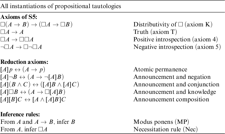
Based on the language $\mathcal {L}_{\textit{PAL}}$ , we introduce the Hilbert-style axiomatic system PAL, which is composed of the axioms and rules of inference in Table 1. As standard, we will write $\vdash _{\textbf {PAL}} A$ , for the formula A is derivable in the Hilbert system PAL.

Table 1

The axiomatisation PAL.

Table 1 Long description

The table is organized into three main sections.

1. Axioms of S 5:

* Distributivity of box (axiom K): box (A yields B) yields (box A yields box B).

* Truth (axiom T): box A yields A.

* Positive introspection (axiom 4): box A yields box box A.

* Negative introspection (axiom 5): lnot box A yields box lnot box A.

2. Reduction axioms:

* Atomic permanence: [A]p if and only if (A yields p).

* Announcement and negation: [A]lnot B if and only if (A yields lnot [A] B).

* Announcement and conjunction: [A](B land C) if and only if ([A]B land [A]C).

* Announcement and knowledge: [A]box B if and only if (A yields box [A]B).

* Announcement composition: [A][B]C if and only if [A land [A]B]C.

3. Inference rules:

* Modus ponens (M P): From A and A yields B, infer B.

* Necessitation rule (Nec): From A, infer box A.

We now present the semantics for PAL by first introducing the notion of standard epistemic model, and consequently the notions of satisfaction of a formula in a model and that of updated model.

Definition 2.3 (Epistemic model).

An epistemic model is a tuple $\mathcal {M}=(W,\sim ,V)$ where W is a set of possible states, $\sim : W \rightarrow \mathcal {P}(W^2)$ is an accessibility relation and $V:P \rightarrow \mathcal {P}(W)$ is a valuation. For a model $\mathcal {M}=(W,\sim ,V)$ and a world $w \in W$ , we call $(\mathcal {M},w)$ a pointed epistemic model, or simply a pointed model.

In this definition, $\sim $ is an equivalence relation, i.e., it is reflexive, transitive, and symmetric.

Definition 2.4 (Semantics of PAL).

Given an epistemic model $\mathcal {M}=(W,\sim ,V)$ , the semantic relation $\vDash $ and the updated model $M_A$ are simultaneously defined by induction as follows:

$$ \begin{align*} &\mathcal{M},w \vDash p & &\text{iff} & &w \in V(p) \\ &\mathcal{M},w \vDash \lnot A & &\text{iff} & &\mathcal{M},w \nvDash A \\ &\mathcal{M},w \vDash A\land B & &\text{iff} & &\mathcal{M},w \vDash A \text{ and } \mathcal{M},w \vDash B \\ &\mathcal{M},w \vDash \square A & &\text{iff} & &\mathcal{M},v \vDash A \text{ for all } v \in W \text{ such that } w \sim v\\ &\mathcal{M},w\vDash[A]B & &\text{iff} & &\text{if }\mathcal{M},w\vDash A \text{ then } \mathcal{M}_A,w\vDash B. \end{align*} $$

StartLayout 1st Row 1st Column Blank 2nd Column script upper M comma w true p 3rd Column Blank 4th Column iff 5th Column Blank 6th Column w element of upper V left parenthesis p right parenthesis 2nd Row 1st Column Blank 2nd Column script upper M comma w true not upper A 3rd Column Blank 4th Column iff 5th Column Blank 6th Column script upper M comma w not true upper A 3rd Row 1st Column Blank 2nd Column script upper M comma w true upper A and upper B 3rd Column Blank 4th Column iff 5th Column Blank 6th Column script upper M comma w true upper A and script upper M comma w true upper B 4th Row 1st Column Blank 2nd Column script upper M comma w true white medium square upper A 3rd Column Blank 4th Column iff 5th Column Blank 6th Column script upper M comma v true upper A for all v element of upper W such that w tilde v 5th Row 1st Column Blank 2nd Column script upper M comma w true left bracket upper A right bracket upper B 3rd Column Blank 4th Column iff 5th Column Blank 6th Column if script upper M comma w true upper A then script upper M Subscript upper A Baseline comma w true upper B period EndLayout

After announcement of $ A $ , the updated model $ \mathcal {M}_A = ( W_{A},\sim _{A}, V_{A}) $ is defined as follows:

$$ \begin{align*} W_{A} &= \lbrace w \in W : \mathcal{M},w \vDash A \rbrace \\ \sim_{A} &= \ \sim \cap\ W_{A} \\ V_{A}(p) &= V(p) \cap W_{A}. \end{align*} $$

StartLayout 1st Row 1st Column upper W Subscript upper A 2nd Column equals left brace w element of upper W colon script upper M comma w true upper A right brace 2nd Row 1st Column tilde Subscript upper A Baseline 2nd Column equals tilde intersection upper W Subscript upper A Baseline 3rd Row 1st Column upper V Subscript upper A Baseline left parenthesis p right parenthesis 2nd Column equals upper V left parenthesis p right parenthesis intersection upper W Subscript upper A Baseline period EndLayout

A formula A is valid, denoted $\vDash _{\textit{PAL}} A$ if, and only if, for all models $\mathcal {M}=(W,\sim ,V)$ and all worlds $w \in W$ , $\mathcal {M},w\vDash A$ . The set of all validities is denoted PAL.

Informally, to define the updated model $ \mathcal {M}_A $ we retain all and only the worlds in which $ A$ is true and leave the accessibility relation between remaining worlds and valuations at those worlds unchanged. In this sense, the effect of the announcement of $ A $ is to restrict the epistemic model to all and only the states where A holds. Therefore, announcements can be seen as epistemic state updaters.

For our purpose, we need to introduce a notation to denote a list of announcements. We do that in the following definition.

Definition 2.5 (List of announcement).

We define a list of announcement $\alpha $ in a public announcement formula $[\alpha ]B$ by induction in the following way:

• $[\epsilon ]B := B$ .
• $[\alpha \cdot A]B := [\alpha ][A]B$ .

By consequence we have

$$ \begin{align*} &\mathcal{M}_\alpha,w \vDash [A]B & &\text{iff} & &\text{if } \mathcal{M}_\alpha,w \vDash A \text{ then } \mathcal{M}_{\alpha \cdot A},w \vDash B. \end{align*} $$

Theorem 2.6 (Soundness and completeness of PAL).

For all formulas $A \in \mathcal L_{\textit{PAL}}$ ,

$$ \begin{align*} \vdash_{\textbf{PAL}} A \quad \text{ if, and only if, } \quad \vDash_{\textit{PAL}} A. \end{align*} $$

Proof. The proof can be found in [Reference van Ditmarsch, Hoek, Kooi and van Der6].

3 Dynamic hypersequents for PAL

In this section, we introduce DHSs, which extend classical hypersequents by incorporating a dynamic mechanism that enables transitions from one hypersequent to another. We introduce them step-by-step, starting from the standard notion of sequent.

Definition 3.1 (Sequent).

A sequent is a syntactic object of the form $M\Rightarrow N$ , where M and N are finite multisets of formulas. We denote sequents by capital greek letters $\Gamma , \Delta , \dots $ . By consequence, occurrences of specific formulas in sequents, e.g., $A, M\Rightarrow N$ or $M\Rightarrow N, A$ , will be denoted by $A, \Gamma $ and $\Gamma , A$ , respectively. Finally, when $\Gamma = M \Rightarrow N$ and $\Delta = P \Rightarrow Q$ , the sequent $M,P \Rightarrow N,Q$ is denoted $\Gamma \Delta $ .

Definition 3.2 (Dynamic sequent).

Let $\Gamma _1,\ldots ,\Gamma _n$ be sequents and $\alpha _1,\ldots ,\alpha _n$ be finite sequences of announcements pairwise distinct, i.e., $\alpha _i\neq \alpha _j$ for all $1\leq i\neq j \leq n$ . Then $\backslash\!\backslash _{\alpha _1}\Gamma _1 \backslash\!\backslash \dots \backslash\!\backslash _{\alpha _n}\Gamma _n$ is a dynamic sequent. For the empty sequence $\epsilon $ we write $\Gamma $ instead of $\backslash\!\backslash _\epsilon \Gamma $ . In particular then $\Gamma $ is a dynamic sequent.

Intuitively, a dynamic sequent represents a world w in some model $\mathcal {M}=(W,\sim ,V)$ , together with its copies in successively updated models $\mathcal {M}_\alpha $ that w belongs to. For instance the dynamic sequent $M\Rightarrow N \backslash\!\backslash _A M' \Rightarrow N'$ represents the world w in the initial model $\mathcal {M}$ as well as in the updated model $\mathcal {M}_A$ .

Note that in a dynamic sequent $X = \Gamma \backslash\!\backslash _{\alpha _1} \Gamma _1 \backslash\!\backslash \dots \backslash\!\backslash _{\alpha _n} \Gamma _n$ , we call $\backslash\!\backslash _\alpha \ \Gamma $ the $\alpha $ -projection of X, or simply the $\alpha $ -sequent. Note that by definition, for any $\alpha $ , the $\alpha $ -projection of X is unique. In particular, we call $\Gamma $ the initial sequent.

Definition 3.3 (Dynamic hypersequent).

Let $X_1,\ldots ,X_n$ be dynamic sequents. Then, $G := X_1 \ \boldsymbol {\mid } \ \dots \ \boldsymbol {\mid } \ X_n$ is a DHS.

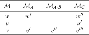
Intuitively, a DHS is the syntactic representation of a model $\mathcal {M}=(W,\sim ,V)$ and its successive updates $\mathcal {M}_\alpha $ . For a better understanding, we can think of the set of updated models as a two-dimensional table, where each row represents a world and its copies (if any) in the successive updated models, and each column represents an updated model, with the different worlds that belong to it. DHSs are a linear representation of such a table. As an example, the following table represents a model $\mathcal {M}$ with three worlds $w, u, v$ , and three updated models obtained from $\mathcal {M}$ by announcing, respectively, A, A and then B, and C.Footnote ¹

Table 2

A four-column table mapping variables w, u, and v to specific mathematical sets M, M sub A, M sub A dot B, and M sub C. See long description.

Table 2 Long description

The table consists of four columns and four rows including the header.

Header Row:

- Column 1: M

- Column 2: M sub A

- Column 3: M sub A dot B

- Column 4: M sub C

Row 2:

- Column 1: Variable w

- Column 2: w prime

- Column 3: Empty

- Column 4: w triple prime

Row 3:

- Column 1: Variable u

- Column 2: Empty

- Column 3: Empty

- Column 4: u prime

Row 4:

- Column 1: Variable v

- Column 2: v prime

- Column 3: v double prime

- Column 4: v triple prime

The following DHS stands for the syntactic representation of the table above, where sequents $\Gamma ,\Delta $ and $\Lambda $ represent worlds $w,u$ and v, respectively:

$$ \begin{align*} \Gamma \backslash\!\backslash_A \Gamma' \backslash\!\backslash_C \Gamma" \ \boldsymbol{\mid} \ \Delta \backslash\!\backslash_C \Delta' \ \boldsymbol{\mid} \ \Lambda \backslash\!\backslash_A \Lambda' \backslash\!\backslash_{A \cdot B} \Lambda" \backslash\!\backslash_C \Lambda"'. \end{align*} $$

In a hypersequent G, if we only consider initial sequents, then we get the syntactic representation of the initial model $\mathcal {M}$ , called initial hypersequent. Similarly, if we only consider $\alpha $ -sequents, we obtain the $\alpha $ projection of G, that is, a representation of the updated model $\mathcal {M}_\alpha $ : this is called $\alpha $ -hypersequent.

Definition 3.4 (Interpretation).

The interpretation $\tau $ of a sequent $M \Rightarrow N$ is the standard one, namely: $(M \Rightarrow N)^\tau := \bigwedge M \rightarrow \bigvee N$ . We extend it to dynamic sequents as follows:

$$ \begin{align*} \backslash\!\backslash_{\alpha_1}\Gamma_1 \backslash\!\backslash \dots \backslash\!\backslash_{\alpha_n} \Gamma_n := [\alpha_1]\Gamma_1^\tau \lor \cdots \lor [\alpha_n]\Gamma_n^\tau, \end{align*} $$

where, for all $1 \leq i \leq n$ , $\alpha _i = A_{i_1}\cdot \dots \cdot A_{i_{k_i}}$ and $[\alpha _i]B = [A_{i_1}]\dots [A_{i_{k_i}}]B$ , for $k_i \in \mathbb N$ .

Finally, we extend the interpretation function $\tau $ to DHSs as follows:

$$ \begin{align*} (X_1 \ \boldsymbol{\mid} \ \cdots \ \boldsymbol{\mid} \ X_n)^\tau := \square X_1^\tau \lor \cdots \lor \square X_n^\tau. \end{align*} $$

We now have all ingredients to introduce the calculus $\mathbf {DHS}_{\textit{PAL}}$ , which is composed by the following axioms and inference rules.

Axioms:

Propositional rules:

Four logical inference rules. Top-left (L-not): G | X alpha M implies N, A all over G | X alpha not A, M implies N. Top-right (R-not): G | X alpha A, M implies N all over G | X alpha M implies N, not A. Bottom-left and bottom-right follow.

Modal rules:

Three logical inference rules. Top-left: L box 1 rule. Top-right: R box rule. Bottom-left: L box 2 rule. Each rule shows a premise over a conclusion separated by a horizontal line.

Inference rule L box 3. Numerator G | X-bar | Y alpha Delta, B 1 and G | X-bar | Y alpha Delta alpha dot B 1 yields B 2 and G | X-bar | Y alpha Delta alpha dot beta A yields all over denominator G | X alpha dot beta box A, Gamma | Y alpha Delta.

Announcement rules:

Two logical inference rules. Rule L dot: G | X alpha M yields N, A alpha dot A M prime yields N prime and G | X alpha M yields N alpha dot A B, M prime yields N prime all over G | X alpha [A]B, M yields N alpha dot A M prime yields N prime.

Dynamic rules:

Four logical inference rules labeled Lat, Rat, New, and Recall. Each rule shows a premise above a horizontal line and a conclusion below, involving variables G, X, M, N, p, and Greek alpha. A condition for Recall is provided at the bottom.

In both the announcement rules (L $[\cdot ]$ ) and (R $[\cdot ]$ ), if the dynamic sequent $\backslash\!\backslash _{\alpha \cdot A}\ M' \Rightarrow N'$ does not occur in the conclusion, we add it to their premises with $M'$ and $N'$ instantiated as empty multisets. So, for example, the rule (L $[\cdot ]$ ) might have the following form:

In the rest of the paper, (L $[\cdot ])_1$ and (R $[\cdot ])_1$ will denote instances of the rules where the dynamic sequent $\backslash\!\backslash _{\alpha \cdot A}\ M' \Rightarrow N'$ occurs in the conclusion; (L $[\cdot ])_2$ and (R $[\cdot ])_2$ will denote instances of the rules where the dynamic sequent $\backslash\!\backslash _{\alpha \cdot A}M' \Rightarrow N'$ does not occur in the conclusion.

We now turn to a more informal discussion of the rules of the calculus. The propositional rules are the standard ones from classical logic, adapted to the DHS framework. The modal rules—(L $\square _1$ ), (L $\square _2$ ), and (R $\square $ )—are essentially those introduced in [Reference Poggiolesi15], though once again reformulated to fit within the DHS setting.

The announcement rules become intuitive when viewed through the Kripke semantics satisfability relation of public announcement formulas. Consider the rules read bottom-up. For (R $[\cdot ]$ ), let $\mathcal {M}=(W,\sim ,V)$ be a model and w be a world of that model represented by the dynamic sequent X. If $[A]B$ is false at $(\mathcal {M}_\alpha ,w)$ , then A must be true at w (so that it can indeed be announced): this is displayed via the sequent $\backslash\!\backslash _\alpha \ A, M \Rightarrow N$ . After this announcement, however, B is false at w in the further updated model $\mathcal {M}_{\alpha \cdot A}$ , which is displayed by the sequent $\backslash\!\backslash _{\alpha \cdot A} \ M'\Rightarrow N',B$ .

Similarly, for (L $[\cdot ]$ ): if $[A]B$ is true at w in $\mathcal {M}_\alpha $ , then one of the following two options must hold: either A is false at $(\mathcal {M}_\alpha ,w)$ , in which case the announcement cannot be made, or else A is true at $(\mathcal {M}_\alpha ,w)$ , so that $w \in \mathcal {M}_{\alpha \cdot A}$ , and B holds at $(\mathcal {M}_{\alpha \cdot A},w)$ . The former case is represented in the left-premise by $\backslash\!\backslash _\alpha \ M \Rightarrow N, A$ while the latter is displayed in the right-premise by $\backslash\!\backslash _{\alpha \cdot A}\ B, M' \Rightarrow N'$ .

The dynamic rules capture important structural properties of models and their updates. Rules (Lat) and (Rat) express atomic permanence: read bottom-up, (Lat), for example, states that if p holds at w in the updated model $\mathcal {M}_{\alpha \cdot A}$ —represented by $\backslash\!\backslash _{\alpha \cdot A}\ p,M' \Rightarrow N'$ —then p must also hold at w in the previous model $\mathcal {M}_\alpha $ —which corresponds to $\backslash\!\backslash _{\alpha }\ p,M \Rightarrow N$ . Rule (New) ensures that if $w \in \mathcal {M}_{\alpha \cdot A}$ , then w must already belong to the previous model $\mathcal {M}_\alpha $ : hence from $\backslash\!\backslash _{\alpha \cdot A}\ M \Rightarrow N$ we get $\backslash\!\backslash _\alpha \Rightarrow $ . Finally, (Recall) requires that if $w \in \mathcal {M}_{\alpha \cdot A}$ —displayed by $\backslash\!\backslash _{\alpha \cdot A}\ M' \Rightarrow N'$ —then A must be true at $(\mathcal {M}_\alpha ,w)$ , which corresponds to $\backslash\!\backslash _\alpha \ A, M \Rightarrow N$ .

Finally, rule (L $\Box _3$ ) should be seen as a dynamic modal rule, since it displays the relationship between knowledge and announcements. It can be understood as follows: for $\square A$ to be true at some world w in some updated model $\mathcal {M}_{\alpha \cdot \beta }$ , every accessible world in $\mathcal {M}_{\alpha \cdot \beta }$ must satisfy A. Hence, for any other world $v\in \mathcal {M}_\alpha $ , either $v\notin \mathcal {M}_{\alpha \cdot \beta }$ , or A is true at v in $\mathcal {M}_{\alpha \cdot \beta }$ . The latter case is represented by the rightmost premise of the rule. The former case, on the other hand, is represented by all the remaining premises: indeed, for $v \in \mathcal {M}_\alpha $ not to belong to $\mathcal {M}_{\alpha \cdot \beta }$ , one of the following must hold (where $\beta = B_1 \dots B_n$ ): $B_1$ is false at $(\mathcal {M}_\alpha ,v)$ , so v does not belong to $\mathcal {M}_{\alpha \cdot B_1}$ , or $v \in \mathcal {M}_{\alpha \cdot B_1}$ but $B_2$ is false at $(\mathcal {M}_{\alpha \cdot B_2},w)$ , etc. This is why (L $\square _3$ ) has $n+1$ premises, when the sequence $\beta $ is composed of n announcements.

As an example, consider the following instance of the rule, where $\beta = B$ and G is empty:

$Logical inference rule L box 3 showing a fraction-style derivation. The numerator contains two complex sequents involving X, Y, alpha, B, and box A, leading to the conclusion in the denominator: X parallel alpha dot B box A, Gamma bar Y parallel a...$

Let $\mathcal {M}=(W,\sim ,V)$ be a model where $W = \lbrace w,v \rbrace $ . Worlds $w, v$ are represented by $X \backslash\!\backslash _{\alpha \cdot B} \square A, \Gamma $ and $Y \backslash\!\backslash _{\alpha } \Delta $ , respectively. Then, we have $w \in W_{\alpha \cdot B}$ (which implies ${w \in W_\alpha }$ ) and $v \in W_{\alpha }$ . For $\mathcal {M}_{\alpha \cdot B},w \vDash \square A$ to hold, either $v \notin W_{\alpha \cdot B}$ or $\mathcal {M}_{\alpha \cdot B}, v \vDash A$ . The first case arises when $\mathcal {M}_\alpha , v \nvDash B$ , which corresponds, in the first premise, to the sequent $\backslash\!\backslash _\alpha \ \Delta ,B$ . The second case is captured, in the second premise, by the sequent $\backslash\!\backslash _{\alpha \cdot B} \, A \Rightarrow $ .

Definition 3.5. Derivations in $\mathbf {DHS}_{\textit{PAL}}$ are defined in the standard way and are denoted by $d, d', etc.$ . The height of a derivation d, denoted $h(d)$ , is also inductively defined in the standard way (see [Reference Troelstra and Schwichtenberg19]). As usual, we write $\vdash _{\mathbf {DHS}_{\textit{PAL}}} G$ to denote that the DHS G is derivable in the calculus $\mathbf {DHS}_{\textit{PAL}}$ .

4 Admissibility of the structural rules and invertibility of the logical rules

In this section, we show that the structural rules of weakening, contraction and merge are hp-admissible, and that all logical rules are hp-invertible. We also introduce new dynamic structural rules and we prove their hp-admissibility.

First of all, we introduce the following notion that will prove useful to define the structural rules.

Definition 4.1. Let $X = \backslash\!\backslash _{\alpha _1} \, \Gamma _1 \backslash\!\backslash \cdots \backslash\!\backslash _{\alpha _n} \Gamma _n$ be a dynamic sequent. The labels of X are all the sequences of announcements that label some sequent in X, i.e., $labels(X)= \lbrace \alpha _1, \ldots , \alpha _n \rbrace $ .

Lemma 4.2. All DHSs of the form $G \ \boldsymbol {\mid } \ X \backslash\!\backslash _\alpha A, M \Rightarrow N, A$ are derivable.

Proof. By standard induction on the complexity of A.

Lemma 4.3. The rule of internal weakening is hp-admissible.

Proof. The proof proceeds by straightforward induction on the height of the derivation of the premise.

Lemma 4.4. The rule of external weakening is hp-admissible:

Proof. The proof proceeds by induction on the height of the derivation of the premise. If G is an axiom, so is $G \ \boldsymbol {\mid } \ X$ . If G is not an axiom, we distinguish cases on the last applied rule $ \mathcal {R}$ : in each of the cases, we apply the inductive hypothesis to the premise(s) of $ \mathcal {R}$ and then use $ \mathcal {R}$ again. We only show one example, whilst the others can be treated similarly.

If the last applied rule is (R $[\cdot ])_2$ , we proceed as follows:

Two logical inference rules separated by a transformation arrow. Left shows derivation d yielding G | Y alpha Gamma, [A]B. Right shows derivation d prime yielding G | Y alpha Gamma, [A]B | X. Both use rule (R[dot]) sub 2.

Lemma 4.5. The rule of dynamic weakening is hp-admissible, where $\alpha \notin labels(X)$ :

Proof. The proof proceeds by induction on the height of the derivation of the premise and is similar to the one of the above lemma. Note that in the inductive step, we may need to use hp-admissibility of (IW) and replace some instances of (L $[\cdot ])_2$ (resp. (R $[\cdot ])_2$ ) by instances of (L $[\cdot ])_1$ (resp. (R $[\cdot ])_1$ ). We provide one example below:

$G | X \\ alpha A, M implies N \\ alpha dot A implies B all over G | X \\ alpha M implies N, [A]B (R[dot]) sub 2$

Here we use the hp-admissibility of (IW) and apply (R $[\cdot ])_2$ to obtain the desired conclusion:

Lemma 4.6. All logical rules are hp-invertible.

Proof. For each rule, the proof proceeds by induction on the height of a derivation of the conclusion.

$-$ Propositional rules: We only show invertibility of (L $\land $ ), because the method is the same for the others. If $G \ \boldsymbol {\mid } \ X \backslash\!\backslash _\alpha A \land B, M \Rightarrow N$ is an axiom, then so is $G\ \boldsymbol {\mid } \ X \backslash\!\backslash _\alpha A,B, M \Rightarrow N$ . Otherwise, we consider the last occurrence of a rule $\mathcal {R}$ in the derivation. If $ \mathcal {R}$ has $A\land B$ as its principal formula, then it must be an occurrence of (L $\land )$ and the premise is precisely $G \ \boldsymbol {\mid } \ X \backslash\!\backslash _\alpha A,B,M \Rightarrow N$ . If $A\land B$ is not principal in $\mathcal {R}$ , we apply the inductive hypothesis to the premise(s) of $\mathcal {R}$ and then use $\mathcal {R}$ again.

$-$ Modal rules: (L $\square _1$ ) and (L $\square _2$ ) are hp-invertible by hp-admissibility of (IW) and (L $\square _3$ ) is hp-invertible by hp-admissibility of (IW) and (DW). We now dwell on the hp-invertibility of (R $\square $ ). If $G \boldsymbol {\mid } X \backslash\!\backslash _\alpha M \Rightarrow N, \square A$ is an axiom, then so is $G \boldsymbol {\mid } X \backslash\!\backslash _\alpha M \Rightarrow N \ \boldsymbol {\mid } \ \backslash\!\backslash _\alpha \Rightarrow A$ . Otherwise, we consider the last occurrence of a rule $\mathcal {R}$ in the derivation. If the principal formula of $\mathcal {R}$ is $\square A$ , then $\mathcal {R}$ is the rule (R $\square $ ) and its premise is precisely what we want, namely $G \boldsymbol {\mid } X \backslash\!\backslash _\alpha M \Rightarrow N \ \boldsymbol {\mid } \ \backslash\!\backslash _\alpha \Rightarrow A$ . If $\square A$ is not principal in $\mathcal {R}$ , we apply the inductive hypothesis to the premise(s) of the rule and then use $\mathcal {R}$ again. We show one example where $\mathcal {R}$ is an occurrence of (L $\square _3$ ).

Inference rule L box 3. Premises d 1 through d n above a line lead to conclusion G | X double-slash alpha Gamma, box A | Y double-slash alpha dot beta box C, Delta. Premises include sequents with box A, B 1, and box C.

$ {\overset {(IH)}{\rightsquigarrow }}$

Logical inference rule L box 3. Premises d sub 1 prime and d sub n prime lead to sequents involving G, X, Gamma, B sub 1, A, Y, and Delta. The conclusion is G | X alpha Gamma | alpha yields A | Y alpha dot beta box C, Delta.

$-$ Announcement rules: We need to consider both versions of each rule. We first consider (R $[\cdot ])_1$ , whilst (L $[\cdot ])_1$ is treated likewise. If $G \boldsymbol {\mid } X \backslash\!\backslash _\alpha \, A, M \Rightarrow N \backslash\!\backslash _{\alpha \cdot A} \, M' \Rightarrow N',B$ is an axiom, then so is $G \boldsymbol {\mid } X \backslash\!\backslash _\alpha \, M \Rightarrow N, [A]B \backslash\!\backslash _{\alpha \cdot A} M' \Rightarrow N'$ . Otherwise, we consider the last applied rule $ \mathcal {R}$ . If $ \mathcal {R}$ has $[A]B$ as its principal formula, then it must be (R $[\cdot ])_1$ and the premise is precisely $G \boldsymbol {\mid } X \backslash\!\backslash _\alpha \, A,M \Rightarrow N \backslash\!\backslash _{\alpha \cdot A} M' \Rightarrow N',B$ . If $[A]B$ is not principal, we apply the inductive hypothesis on the premise(s) and then $ \mathcal {R}$ again. We show one case with (L $\square _3$ ), whilst others are treated analogously. In the following, $\overline {Y}$ denotes $Y \backslash\!\backslash _{\alpha \cdot A \cdot \beta } \square C,\Delta $ :

Logical inference rule L(box 3). Premises d 1 through d k lead to a conclusion. G | X alpha Gamma, [A]B alpha dot A Gamma prime | Y alpha dot A dot beta box C, Delta.

$ {\overset {(IH)}{\rightsquigarrow }}$

Inference rule L(box 3). Premises d sub 1 prime and d sub k prime lead to G | X alpha A, Gamma alpha dot A Gamma prime, B, B sub 1 | Y-bar ... G | X alpha A, Gamma alpha dot A Gamma prime, B alpha dot A dot beta C implies | Y-bar all over conclusion.

We now turn to (R $[\cdot ])_2$ , while (L $[\cdot ])_2$ is treated likewise. The proof proceeds similarly, except when the dynamic sequent $\backslash\!\backslash _{\alpha \cdot A} \ \Gamma '$ appears in the premise(s) of $\mathcal {R}$ . In such cases, we use hp-invertibility of (R $[\cdot ])_1$ on the premise(s) displaying $\backslash\!\backslash _{\alpha \cdot A} \ \Gamma '$ instead of the inductive hypothesis. Afterwards, we might need to apply a different version of rule $\mathcal {R}$ , i.e., (L $[\cdot ])_1$ (resp. (R $[\cdot ])_1$ ) instead of (L $[\cdot ])_2$ (resp. (R $[\cdot ])_2$ ), and (L $\square _2$ ) instead of (L $\square _3$ ). We provide some examples, whilst other cases can be treated similarly.

If $\mathcal {R}$ is an occurrence of (L $[\cdot ])_2$ , we proceed as follows:

Inference rule with premises d sub 1 and d sub 2 above a line and a conclusion below. Premises: G | X double-slash alpha Gamma, [A]B, A and G | X double-slash alpha Gamma, [A]B double-slash alpha dot A C implies. Conclusion: G | X double-slash alpha [A]C, Gamma, [A]B.

We apply the inductive hypothesis on the left-hand premise, to obtain $G\ \boldsymbol {\mid } \ X \backslash\!\backslash _\alpha \ A,\Gamma ,A \backslash\!\backslash _{\alpha \cdot A} \ \Rightarrow B$ while we use hp-invertibility of (R $[\cdot ])_1$ on the right-hand premise to get $G \ \boldsymbol {\mid } \ X \backslash\!\backslash _\alpha \ A,\Gamma \backslash\!\backslash _{\alpha \cdot A} \ C \Rightarrow B$ . We then apply (L $[\cdot ])_1$ to obtain the desired conclusion:

Logical inference rule with premises d sub 1 prime and d sub 2 prime. G | X double-slash alpha A, Gamma, A double-slash alpha dot A implies B and G | X double-slash alpha A, Gamma double-slash alpha dot A C implies B yield the conclusion.

When $\mathcal {R}$ is an occurrence of (L $\square _3$ ) with two premises as below:

$Inference rule L(box sub 3). Premises d sub 1 and d sub 2 above a line yield conclusion G | X \\ alpha M implies N, [A]B | Y \\ alpha dot A box C, Delta. Premises involve complex sequents with alpha and box operators.$

we consider the right-hand premise only: we apply hp-invertibility of (R $[\cdot ])_1$ on it and then use (L $\square _2$ ) instead of (L $\square _3$ ), to getFootnote ³ :

$Logical inference rule with vertical ellipsis d sub 2 prime above a premise G | X \\ alpha A, M implies N \\ alpha dot A C implies B | Y \\ alpha dot A box C, Delta all over conclusion G | X \\ alpha A, M implies N \\ alpha dot A implies B | Y \\ A box C, Delta L(box 2).$

Eventually, when $\mathcal {R}$ is an occurrence of (New) where $\backslash\!\backslash _{\alpha \cdot A} \ \Gamma '$ appears in the premise, hp-invertibility of (R $[\cdot ])_1$ directly provides the conclusion, with no need for further application of (New), as shown below:

Logical inference rule with premise d over conclusion labeled New. A dashed arrow with R dot 1 2 points to a second structure with premise d prime over a sequent involving G, X, A, Gamma, and B with alpha and C subscripts.

$-$ Dynamic rules: (Lat) and (Rat), as well as (Recall) are hp-invertible by hp-admissibility of (IW). (New) is hp-invertible by hp-admissibility of (DW).

From now on, for any given rule $\mathcal {R}$ , we denote by $\mathcal {R}^\star $ the inverted rule,Footnote ⁵ that is derivable, by Lemma 4.6.

As is standard in a hypersequent framework, there is a merge rule that can be shown to be hp-admissible. To define the rule, we need to introduce the symbol $\otimes $ for $X\otimes Y$ , which intuitively combines two DHSs X and Y in the following way: all dynamic sequents labelled by the same sequence of announcements $\alpha $ are merged pairwise, while the remaining dynamic sequents are simply juxtaposed.

Definition 4.7. Let X and Y be two DSs, then $X \otimes Y$ is inductively defined as follows:

• if X is empty (resp. Y is empty) then $X \otimes Y := Y$ (resp. $X \otimes Y := X$ );
• if $X= X' \backslash\!\backslash _{\alpha }\, M \Rightarrow N$ and $Y= Y' \backslash\!\backslash _{\alpha } \, P \Rightarrow Q$ then $X \otimes Y := X'\otimes Y' \backslash\!\backslash _{\alpha } M,P\Rightarrow N,Q$ ;
• if $X= X' \backslash\!\backslash _{\alpha } M \Rightarrow N$ and $Y= Y' \backslash\!\backslash _{\beta } P \Rightarrow Q$ , where $\alpha \notin \ labels(Y')$ and $\beta \notin \ labels(X')$ , then $X \otimes Y := X'\otimes Y' \backslash\!\backslash _{\alpha } M\Rightarrow N \backslash\!\backslash _{\beta }P \Rightarrow Q$ .

For instance, if $X = \Gamma \backslash\!\backslash _{A} \Gamma ' \backslash\!\backslash _{A\cdot B} \Gamma "$ and $Y= \Delta \backslash\!\backslash _A \Delta ' \backslash\!\backslash _B \Delta " \backslash\!\backslash _{B\cdot A} \Delta "'$ , then $X \otimes Y = \Gamma \Delta \backslash\!\backslash _A \Gamma '\Delta ' \backslash\!\backslash _{A\cdot B} \Gamma " \backslash\!\backslash _B \Delta " \backslash\!\backslash _{B\cdot A} \Delta "'$ .

Lemma 4.8. The rule of Merge is hp-admissible:

Proof. The proof proceeds by induction on the height of the derivation of the premise. If $G \boldsymbol {\mid } X \backslash\!\backslash _\alpha M \Rightarrow N \ \boldsymbol {\mid } \ Y \backslash\!\backslash _\alpha P \Rightarrow Q$ is an axiom, so is $G \boldsymbol {\mid } X \otimes Y \backslash\!\backslash _\alpha M,P \Rightarrow N,Q$ . Otherwise, we consider the last applied rule $ \mathcal {R}$ : we apply the inductive hypothesis to the premise(s) of $ \mathcal {R}$ and then use $ \mathcal {R}$ again. We only show two paradigmatic examples.

If $\mathcal {R}$ is an occurrence of (R $\square $ ):

Logical derivation. Left side d premise G | X alpha Gamma | Y alpha Delta | alpha implies A over conclusion G | X alpha Gamma, box A | Y alpha Delta. Squiggly arrow with I H maps to right side d prime premise and conclusion with tensor products.

If $ { \mathcal {R}}$ is an occurrence of (L $ {\square _3}$ ) of the following shape:

Logical inference rule L box 3. Premises d 1 through d n above a horizontal line lead to the conclusion G | X alpha Gamma | Y alpha Delta alpha dot beta box A, Delta prime below the line.

we simply apply the inductive hypothesis to the rightmost premise, and conclude with (L $\square _1$ ):

Logical derivation step labeled (L box 1) showing a premise with A and box A, and a conclusion with only box A, following a vertical ellipsis d’ sub n.

Lemma 4.9. The rules of contraction are hp-admissible:

$Left rule (L C) numerator G | X \\ alpha A, A, M implies N all over denominator G | X \\ alpha A, M implies N. Right rule (R C) numerator G | X \\ alpha M implies N, A, A all over denominator G | X \\ alpha M implies N, A.$

Proof. We simultaneously prove the hp-admissibility of (LC) and (RC) by induction on the height of the derivation of the premise of each rule. If $G \boldsymbol {\mid } X \backslash\!\backslash _\alpha A, A, M\Rightarrow N$ and $G \boldsymbol {\mid } X \backslash\!\backslash _\alpha M \Rightarrow N, A, A$ are axioms, then so are $G \boldsymbol {\mid } X \backslash\!\backslash _\alpha A, M \Rightarrow N$ and $G \boldsymbol {\mid } X \backslash\!\backslash _\alpha M \Rightarrow N, A$ . Else, we distinguish cases on the last applied rule $ \mathcal {R}$ . If neither of the occurrences of A is principal, we apply the inductive hypothesis to the premise(s) of $ \mathcal {R}$ , and then use $ \mathcal {R}$ again. If one of the occurrence of A is principal, we start from the premise(s) of $ \mathcal {R}$ and use the hp-invertibility of the rules before applying the inductive hypothesis; then we use $ \mathcal {R}$ again. We only show one example, while the others can be treated similarly.

If the last applied rule is (R $[\cdot ])_2$ , we first use hp-invertibility of (R $[\cdot ])_1$ , then we apply the inductive hypothesis twice, and eventually we use (R $[\cdot ])_2$ again:

$Logical derivation showing a rule R dot transformation. Left side has a fraction with d sub 1 above G | X double-slash alpha A, Gamma [A] B double-slash alpha dot A implies B, all over G | X double-slash alpha Gamma, [A] B, [A] B.$

We end this section by proving the admissibility of the rule $New^{A}$ , which will be crucial to prove the admissibility of the Cut-rule.

Lemma 4.10. The rule New $^{A}$ is admissible:

Proof. We proceed by induction on the height of the derivation of the premise. If $G \boldsymbol {\mid } X \backslash\!\backslash _\alpha A, M \Rightarrow N \backslash\!\backslash _{\alpha \cdot A} \Rightarrow $ is an axiom then so is $G \boldsymbol {\mid } X \backslash\!\backslash _\alpha A, M \Rightarrow N$ . If $G \boldsymbol {\mid } X \backslash\!\backslash _\alpha A, M \Rightarrow N \backslash\!\backslash _{\alpha \cdot A} \Rightarrow $ is of the form $G \boldsymbol {\mid } X \backslash\!\backslash _\alpha A, M \Rightarrow N \backslash\!\backslash _{\alpha \cdot A} \Rightarrow \backslash\!\backslash _{\alpha \cdot A \cdot B} \, M' \Rightarrow N'$ —namely the dynamic sequent X contains a sequent of the form $\backslash\!\backslash _{\alpha \cdot A \cdot B} \, M' \Rightarrow N'$ —we simply apply (New) to obtain the desired conclusion:

$G | X \\ alpha A, M implies N \\ alpha dot A implies \\ alpha dot A dot B M prime implies N prime all over G | X \\ alpha A, M implies N \\ alpha dot A dot B M prime implies N prime (New)$

Finally, if $G \boldsymbol {\mid } X \backslash\!\backslash _\alpha A, M \Rightarrow N \backslash\!\backslash _{\alpha \cdot A} \Rightarrow $ is neither an axiom nor of the form indicated above, we consider the last applied rule $ \mathcal {R}$ . If $ \mathcal {R}$ is an application of a right-rule, we apply the inductive hypothesis to the premise(s) of $ \mathcal {R}$ and then use $ \mathcal {R}$ again, as in the example below, where $\mathcal {R}$ is an occurrence of (R $\square $ ):

Logical derivation showing G | X alpha A, M implies N alpha dot A implies | alpha implies B over G | X alpha A, M implies N, box B alpha dot A implies. This transforms via I H to a simplified version with d prime and box B.

If $ \mathcal {R}$ is an application of a left-rule that does not involve neither A nor the dynamic sequent $\backslash\!\backslash _{\alpha \cdot A} \Rightarrow $ , we reason as before. Here is an example with (L $[\cdot ]$ ):

Two-part logical derivation showing inference rules labeled L dot. Top rule has premises d 1 and d 2 leading to a conclusion. A squiggly arrow labeled I H points to a second rule with premises d prime 1 and d prime 2.

If $\mathcal {R}$ is an application of a left-rule that does involve either A or the dynamic sequent $\backslash\!\backslash _{\alpha \cdot A} \Rightarrow $ , then we obtain the desired result using hp-admissibility of weakening and contraction, applying the inductive hypothesis or directly using $\mathcal {R}$ again.

We only show the most significant cases. $- \ \mathcal {R}$ is an application of (L $\square _3$ ) involving $\backslash\!\backslash _{\alpha \cdot A} \Rightarrow $ , with active dynamic sequent $\backslash\!\backslash _{\alpha \cdot A \cdot \beta } \square C, \Delta $ where $\beta = B_1 \dots B_n$ , as below:

Logical inference rule (L□3) showing premises d1 and dn+1 leading to a conclusion with hypersequents G, X, Γ, Y, and Δ, deriving the boxed formula □C within the context α·A·β.

we apply the inductive hypothesis on all the premises except the leftmost, and use $G \boldsymbol {\mid } X \backslash\!\backslash _\alpha A, \Gamma , A \ \boldsymbol {\mid } \ Y \backslash\!\backslash _{\alpha \cdot A \cdot \beta } \square C, \Delta $ (that is derivable by Lemma 4.2) as a first premise to apply (L $\square _3$ ) with $n+2$ premises:

Inference rule L box 3. Premises d 1 and d prime n+1 lead to G | X alpha A, Gamma, A | Y-bar and G | X alpha A, Gamma alpha A implies B 1 | Y-bar through G | X alpha A, Gamma alpha A beta C implies | Y-bar all over G | X alpha A, Gamma | Y alpha A beta box C, Delta.

$-\ \mathcal {R}$ is an application of (L $[\cdot ])$ where A is the principal formula:

Inference rule with premises d sub 1 and d sub 2 over a horizontal line. G | X double-slash alpha M yields N, A double-slash [A]B yields and G | X double-slash alpha M yields N double-slash [A]B yields double-slash alpha dot A B yields.

We first use the hp-admissibility of (IW) to get

$$ \begin{align*} &\vdots \ d_1' & &\vdots \ d_2' \\ \quad G \boldsymbol{\mid} X \backslash\!\backslash_{\alpha} [A]B,M &\Rightarrow N, A \ \backslash\!\backslash_{[A]B} \Rightarrow \quad &G \boldsymbol{\mid} X \backslash\!\backslash_\alpha [A]B, M \Rightarrow &N \ \backslash\!\backslash_{[A]B} \Rightarrow \backslash\!\backslash_{\alpha \cdot A} \ B \Rightarrow \end{align*} $$

then we apply the inductive hypothesis, use (L $[\cdot ])$ and then hp-admissibility of (LC) to conclude:

Logical inference rule L dot with premises d sub 1 double prime and d sub 2 double prime leading to G | X backslash backslash alpha [A]B, [A]B, M yields N, which by rule L C simplifies to G | X backslash backslash alpha [A]B, M yields N.

5 Soundness and completeness

In this section, we show that $\mathbf {DHS}_{\textit{PAL}}$ is sound and complete.

Theorem 5.1 (Soundness).

For all formulas $A \in \mathcal L_{\textit{PAL}}$ , if $\vdash _{\mathbf {DHS}_{\textit{PAL}}} \Rightarrow A$ then $\vDash _{\textit{PAL}} A$ .

Proof. We need to show that axioms are valid and that all rules are correct, i.e., that they preserve validity. As for the axioms, this is straightforward. As for the rules, for the sake of clarity, we only present in detail the case of the rule (R $[\cdot ])_1$ . The other rules can be treated similarly.

For (R $[\cdot ])_1$ , let $\alpha = A_1 \dots A_n$ and suppose $\vDash (G \boldsymbol {\mid } X \backslash\!\backslash _\alpha A, M \Rightarrow N \backslash\!\backslash _{\alpha \cdot A} M' \Rightarrow N',B)^\tau $ but $\nvDash (G \boldsymbol {\mid } X \backslash\!\backslash _\alpha M \Rightarrow N, [A]B \backslash\!\backslash _{\alpha \cdot A} M' \Rightarrow N')^\tau $ . Then, there are a model $\mathcal {M}=(W,\sim ,V)$ and a world $w\in W$ such that

$$ \begin{align*} \mathcal{M},w \nvDash G^\tau \lor \square (X^\tau \lor [\alpha] (\bigwedge M \rightarrow \bigvee N \lor [A]B) \lor [\alpha][A](\bigwedge M' \rightarrow \bigvee N') \end{align*} $$

so there is $u\in W$ such that $w\sim u$ and:

$$ \begin{align*} (1) \quad &\mathcal{M},u \nvDash X^\tau. \\ (2) \quad &\mathcal{M},u \nvDash [\alpha](\bigwedge M \rightarrow \bigvee N \lor [A]B).\\ (3)\quad &\mathcal{M},u \nvDash [\alpha][A](\bigwedge M' \rightarrow \bigvee N'). \end{align*} $$

StartLayout 1st Row 1st Column left parenthesis 1 right parenthesis 2nd Column script upper M comma u not true upper X Superscript tau Baseline period 2nd Row 1st Column left parenthesis 2 right parenthesis 2nd Column script upper M comma u not true left bracket alpha right bracket left parenthesis and upper M right arrow or upper N or left bracket upper A right bracket upper B right parenthesis period 3rd Row 1st Column left parenthesis 3 right parenthesis 2nd Column script upper M comma u not true left bracket alpha right bracket left bracket upper A right bracket left parenthesis and upper M Superscript prime Baseline right arrow or upper N Superscript prime Baseline right parenthesis period EndLayout

From $(3)$ , we get $\mathcal {M},u \vDash A_1, \mathcal {M}_{A_1},u \vDash A_2, \ldots , \mathcal {M}_\alpha , u \vDash A$ and $\mathcal {M}_{\alpha \cdot A} \nvDash \bigwedge M' \rightarrow \bigvee N'$ . From $(2)$ we get $\mathcal {M}_\alpha ,u \vDash \bigwedge M$ and $\mathcal {M}_{\alpha },u \nvDash [A]B$ . From that and $\mathcal {M}_\alpha , u \vDash A$ , we conclude that $\mathcal {M}_{\alpha \cdot A},u \nvDash B$ .

However, since $\vDash (G \boldsymbol {\mid } X \backslash\!\backslash _\alpha A,M \Rightarrow N \backslash\!\backslash _{\alpha \cdot A} M' \Rightarrow N', B)^\tau $ and $\mathcal {M},w \nvDash G^\tau $ , necessarily

$$ \begin{align*} \mathcal{M},w \vDash \square (X^\tau \lor [\alpha](A \land \bigwedge M \rightarrow \bigvee N) \lor [\alpha][A](\bigwedge M' \rightarrow \bigvee N' \lor B)). \end{align*} $$

Now, because $\mathcal {M},u \nvDash X^\tau $ , either $\mathcal {M},u \vDash [\alpha ](A \land \bigwedge M \rightarrow \bigvee N)$ or $M,u \vDash [\alpha ][A] (\bigwedge M' \rightarrow \bigvee N' \lor B)$ . In the first case, we get a contradiction because $\mathcal {M}_\alpha ,u \vDash \bigwedge M$ and $\mathcal {M}_\alpha ,u \vDash A$ but $\mathcal {M}_\alpha ,u \nvDash \bigvee N$ . In the other case, we get a contradiction from $\mathcal {M}_{\alpha \cdot A},u \nvDash \bigwedge M' \rightarrow \bigvee N'$ and $\mathcal {M}_{\alpha \cdot A},u \nvDash B$ which implies ${\mathcal {M}_{\alpha \cdot A} \nvDash \bigwedge M' \rightarrow \bigvee N' \lor B}$ , hence $M,u \nvDash [\alpha ][A](\bigwedge M' \Rightarrow \bigvee N' \lor B)$ .

Therefore $\vDash (G \boldsymbol {\mid } X \backslash\!\backslash _\alpha M \Rightarrow N,[A]B \backslash\!\backslash _{\alpha \cdot A} M' \Rightarrow N')^\tau $ .

We now move to the completeness of the calculus. In order to prove that $\mathbf {DHS}_{\textit{PAL}}$ is complete with respect to PAL, we need to show that all axioms of PAL are derivable, as well as that the inference rules of PAL are admissible. This can be standardly carried out except for the case of the axiom of announcement composition, which requires us to show a derivability lemma (see Lemma 5.3). On the other hand, in order to prove this derivability lemma, we first need an enhanced notion of complexity of formulas, i.e., a notion of complexity of formulas that is relative to the sequents formulas belong to in the context of a DHS.Footnote ⁶ We thus also introduce the notion of DHS-complexity in Definition 5.2. Finally, note that many other calculi for PAL (e.g., [Reference Balbiani, van Ditmarsch, Herzig and de Lima3, Reference Nomura, Sano and Tojo13]) require some preliminary lemmas in order to show a completeness result; hence our procedure is standard in the context of proof theory for PAL.

Definition 5.2 (DHS-complexity).

The DHS-complexity of a formula A relatively to a sequence of announcements $\alpha $ , $c(A,\alpha )$ , is defined as

$$ \begin{align*} c(A,\alpha) := c(A) + c(\alpha), \end{align*} $$

where $c(A)$ is inductively defined as follows:

$$ \begin{align*} c(p)&:= 1 \quad \text{ for } p\in P \\ c(\lnot A) &:= c(A) + 1 & c(\square A) &:= c(A) + 1\\ c(A \land B) &:= c(A) + c(B) +1 & c([A]B) &:= c(A) + c(B) + 1, \end{align*} $$

StartLayout 1st Row 1st Column c left parenthesis p right parenthesis 2nd Column colon equals 1 for p element of upper P 2nd Row 1st Column c left parenthesis not upper A right parenthesis 2nd Column colon equals c left parenthesis upper A right parenthesis plus 1 3rd Column c left parenthesis white medium square upper A right parenthesis 4th Column colon equals c left parenthesis upper A right parenthesis plus 1 3rd Row 1st Column c left parenthesis upper A and upper B right parenthesis 2nd Column colon equals c left parenthesis upper A right parenthesis plus c left parenthesis upper B right parenthesis plus 1 3rd Column c left parenthesis left bracket upper A right bracket upper B right parenthesis 4th Column colon equals c left parenthesis upper A right parenthesis plus c left parenthesis upper B right parenthesis plus 1 comma EndLayout

whilst $c(\alpha )$ is inductively defined as follows:

$$ \begin{align*} c(\epsilon) &:= 0 & c(\alpha \cdot A) &:= c(\alpha) + c(A). \end{align*} $$

Lemma 5.3. Let $A, B, C$ be formulas of $\mathcal L_{\textit{PAL}}$ , and $\alpha ,\beta $ be finite sequences of announcements. Then, the following DHSs are derivable:

$$ \begin{align*} (1) \quad &G \ \boldsymbol{\mid} \ X \backslash\!\backslash_{\alpha\cdot A \cdot B \cdot \beta}\ C, M \Rightarrow N \backslash\!\backslash_{\alpha \cdot A\land[A]B \cdot \beta} \ M' \Rightarrow N',C. \\ (2) \quad &G \ \boldsymbol{\mid} \ X \backslash\!\backslash_{\alpha\cdot A \cdot B \cdot \beta} \ M \Rightarrow N, C \backslash\!\backslash_{\alpha \cdot A\land[A]B \cdot \beta} \ C, M' \Rightarrow N'. \end{align*} $$

Proof. We simultaneously prove that $(1)$ and $(2)$ are derivable by induction on the sum of the DHS-complexity of each occurrence of C, denoted $\overline {c}(C):= c(C, \alpha \cdot A \cdot B \cdot \beta ) + c(C, \alpha \cdot A \land [A]B \cdot \beta )$ .

Without loss of generality, we prove the result for empty G, X and $\alpha $ . In the following, $\beta = B_1 \cdot B_2 \dots B_{n-1}$ and we write $\varphi $ for $A \land [A]B$ . We distinguish the following cases, where we only present the details for $(1)$ , whilst $(2)$ is treated similarly.

$\bullet $ Case $C= p$ . To derive $(1)$ , we (bottom-up) apply $2\times n$ times (New) to go from $\backslash\!\backslash _{\varphi \cdot \beta } \ \Gamma $ to $\backslash\!\backslash _\epsilon \ \Gamma '$ and from $\backslash\!\backslash _{A\cdot B \cdot \beta } \ \Delta $ to $\backslash\!\backslash _{A} \ \Delta '$ , then we apply $n+1$ times (Rat) and n times (Lat) to obtain an axiom with $p\Rightarrow p$ . We write $\mathcal {R}^\ast $ when we apply several times rule $\mathcal {R}$ :

A proof tree equation. Top premises derive A implies A wedge [A]B double-slash A B implies double-slash A dot B implies C. Successive steps apply rules R dot, R wedge, and R arrow to reach the conclusion implies [A wedge [A]B]C arrow [A][B]C.

$\bullet $ Case $C =\lnot C_1$ . Since $\overline {c}( C_1) < \overline {c}(\lnot C_1)$ , we apply the inductive hypothesis. Then, we simply apply (L $\lnot $ ) and (R $\lnot $ ). This is straightforward.

$\bullet $ Case $C = C_1 \land C_2$ . We can apply the inductive hypothesis because $\overline {c}(C_i) < \overline {c}(C_1 \land C_2)$ for $i \in \lbrace 1, 2 \rbrace $ . Then, we apply admissibility of (IW) and use (L $\land $ ) and (R $\land $ ). This is straightforward. $\bullet $ Case $C = \square C_1$ . Note that $\overline {c}(C_1) < \overline {c}(\square C_1)$ and, for all $\beta '\cdot B_i \subseteq \beta $ , $c(B_i, A \cdot B \cdot \beta ') + c(B_i, A \land [A]B \cdot \beta ') < \overline {c}(\square C_1)$ . This allows us to use the inductive hypothesis to obtain the following DHSs:

$$ \begin{align*} (1) \quad &\backslash\!\backslash_{A \cdot B} \Rightarrow B_1 \backslash\!\backslash_\varphi B_1 \Rightarrow \\ (2) \quad &\backslash\!\backslash_{A \cdot B \cdot B_1} \Rightarrow B_2 \backslash\!\backslash_{\varphi \cdot B_1} B_2 \Rightarrow \\ \vdots \ \quad & \\ (n-1) \quad &\backslash\!\backslash_{A \cdot B \dots B_{n-2}} \Rightarrow B_{n-1} \backslash\!\backslash_{\varphi \dots B_{n-2}} B_{n-1} \Rightarrow \\ (n) \quad &\backslash\!\backslash_{A \cdot B \cdot \beta} C_1 \Rightarrow \backslash\!\backslash_{\varphi \cdot\beta} \Rightarrow C_1. \end{align*} $$

StartLayout 1st Row 1st Column left parenthesis 1 right parenthesis 2nd Column set minus set minus dot dot AB right double arrow upper B 1 minus set minus Subscript phi Baseline upper B 1 right double arrow 2nd Row 1st Column left parenthesis 2 right parenthesis 2nd Column set minus set minus dot dot dot ABB 1 right double arrow upper B 2 minus set minus Subscript phi dot upper B 1 Baseline upper B 2 right double arrow 3rd Row 1st Column vertical ellipsis 2nd Column Blank 4th Row 1st Column left parenthesis n minus 1 right parenthesis 2nd Column set minus set minus Underscript upper A dot upper B ellipsis upper B Subscript n minus 2 Baseline Endscripts right double arrow upper B Subscript n minus 1 Baseline minus set minus Underscript phi ellipsis upper B Subscript n minus 2 Baseline Endscripts upper B Subscript n minus 1 Baseline right double arrow 5th Row 1st Column left parenthesis n right parenthesis 2nd Column set minus set minus Subscript upper A dot upper B dot beta Baseline upper C 1 right double arrow set minus set minus dot dot phi beta right double arrow upper C 1 period EndLayout

By admissibility of (IW), (EW) and (DW), from each $(i)$ we get the following $(i')$ :

$$ \begin{align*} (1)' \ &\backslash\!\backslash_{A \cdot B \cdot \beta} \square C_1, \Gamma \backslash\!\backslash_{\varphi \cdot \beta} \Gamma' \ \boldsymbol{\mid} \ A \Rightarrow \backslash\!\backslash_A B \Rightarrow \backslash\!\backslash_{A \cdot B} \Rightarrow B_1 \backslash\!\backslash_\varphi B_1 \Rightarrow \backslash\!\backslash \cdots \backslash\!\backslash_{\varphi \cdot \beta} \Rightarrow C_1 \\ (2)' \ &\backslash\!\backslash_{A \cdot B \cdot \beta} \square C_1, \Gamma \backslash\!\backslash_{\varphi \cdot \beta} \Gamma' \ \boldsymbol{\mid} \ A \Rightarrow \backslash\!\backslash_A B \Rightarrow \backslash\!\backslash_{A \cdot B \cdot B_1} \Rightarrow B_2 \backslash\!\backslash_{\varphi} B_1 \Rightarrow \backslash\!\backslash_{\varphi \cdot B_1} B_2 \Rightarrow \backslash\!\backslash \cdots \backslash\!\backslash_{\varphi \cdot \beta} \Rightarrow C_1 \\ \vdots \quad & \\ (n)' \ &\backslash\!\backslash_{A \cdot B \cdot \beta} \square C_1, \Gamma \backslash\!\backslash_{\varphi \cdot \beta} \Gamma' \ \boldsymbol{\mid} \ A \Rightarrow \backslash\!\backslash_A B \Rightarrow \backslash\!\backslash_{A\cdot B \cdot \beta} C_1 \Rightarrow \backslash\!\backslash_\varphi B_1 \Rightarrow \backslash\!\backslash \cdots \backslash\!\backslash_{\varphi \cdot \beta} \Rightarrow C_1. \end{align*} $$

StartLayout 1st Row 1st Column left parenthesis 1 right parenthesis prime 2nd Column set minus set minus dot dot dot AB beta white medium square upper C 1 comma normal upper Gamma minus set minus Subscript phi dot beta Baseline normal upper Gamma Superscript prime Baseline bold vertical bar upper A right double arrow set minus set minus Subscript upper A Baseline upper B right double arrow set minus set minus dot dot AB right double arrow upper B 1 minus set minus Subscript phi Baseline upper B 1 right double arrow set minus set minus midline horizontal ellipsis set minus set minus Subscript phi dot beta Baseline right double arrow upper C 1 2nd Row 1st Column left parenthesis 2 right parenthesis prime 2nd Column set minus set minus dot dot dot AB beta white medium square upper C 1 comma normal upper Gamma minus set minus Subscript phi dot beta Baseline normal upper Gamma Superscript prime Baseline bold vertical bar upper A right double arrow set minus set minus Subscript upper A Baseline upper B right double arrow set minus set minus dot dot dot ABB 1 right double arrow upper B 2 minus set minus Subscript phi Baseline upper B 1 right double arrow set minus set minus Subscript phi dot upper B 1 Baseline upper B 2 right double arrow set minus set minus midline horizontal ellipsis set minus set minus Subscript phi dot beta Baseline right double arrow upper C 1 3rd Row 1st Column vertical ellipsis 2nd Column Blank 4th Row 1st Column left parenthesis n right parenthesis prime 2nd Column set minus set minus dot dot dot AB beta white medium square upper C 1 comma normal upper Gamma minus set minus Subscript phi dot beta Baseline normal upper Gamma Superscript prime Baseline bold vertical bar upper A right double arrow set minus set minus Subscript upper A Baseline upper B right double arrow set minus set minus Subscript upper A dot upper B dot beta Baseline upper C 1 right double arrow set minus set minus Subscript phi Baseline upper B 1 right double arrow set minus set minus midline horizontal ellipsis set minus set minus Subscript phi dot beta Baseline right double arrow upper C 1 period EndLayout

To apply (L $\square _3$ ) with $\backslash\!\backslash _{A\cdot B\cdot \beta } \square C_1, \Gamma '$ , we need $n+1$ premises, since the sequence of announcements here is $B \cdot B_1 \dots B_{n-1}$ . Hence, we also need the following DHS, that is derivable by Lemma 4.2:

$$ \begin{align*} (0)' \quad \backslash\!\backslash_{A \cdot B \cdot \beta} \square C_1, \Gamma \backslash\!\backslash_{\varphi \cdot \beta} \Gamma' \ \boldsymbol{\mid} \ A \Rightarrow \backslash\!\backslash_A B \Rightarrow B \backslash\!\backslash_\varphi B_1 \Rightarrow \backslash\!\backslash \cdots \backslash\!\backslash_{\varphi \cdot \beta} \Rightarrow C_1. \end{align*} $$

We now apply (L $\square _3$ ) to $(0)'-(n)'$ and continue the derivation as follows, where $X := \backslash\!\backslash _{A\cdot B\cdot \beta } \ \square C_1, \Gamma \backslash\!\backslash _{\varphi \cdot \beta }\ \Gamma '$ :

A multi-step logical proof tree starting with premises (0) prime to (n) prime. It uses horizontal lines to separate steps, applying rules like L box 3, L dot, L wedge, Recall, New, and R box to derive a final sequent at the bottom.

$\bullet $ Case $C=[C_1]C_2$ . We use the inductive hypothesis and admissibility of (DW). Note that the inductive hypothesis applies because $\overline {c}(C_1) < \overline {c}([C_1]C_2)$ and $c(C_2, A \cdot B \cdot \beta \cdot C_1) + c(C_2, A \land [A] B \cdot \beta \cdot C_1) < \overline {c}([C_1]C_2)$ :

A formal logic proof tree deriving the implication arrow open bracket A and open bracket A close bracket B close bracket C arrow open bracket A close bracket open bracket B close bracket C using rules R dot, R wedge, and R arrow.

Note that Lemma 5.3 can be understood as a way of identifying dynamic sequents labelled by $A\cdot B$ and those labelled by $A \land [A]B$ (and more generally by $\alpha \cdot A \cdot B \cdot \beta $ and by $\alpha \cdot A \land [A]B \cdot \beta $ ). This result has a semantic counterpart. Indeed, it can be proved that, for all models $\mathcal {M}=(W,\sim ,V)$ and all formulas $A,B$ , $W_{A\cdot B}= W_{A \land [A]B}$ (see, for instance, [Reference van Ditmarsch, Hoek, Kooi and van Der6]).

Theorem 5.4 (Completeness).

For all formulas $A \in \mathcal L_{\textit{PAL}}$ , if $\vDash _{\textit{PAL}} A$ then $\vdash _{\mathbf {DHS}_{\textit{PAL}}} \Rightarrow A$ .

Proof. Since PAL is complete w.r.t. the standard semantics of PAL, it is sufficient to demonstrate that all axioms of PAL are derivable in $\mathbf {DHS}_{\textit{PAL}}$ and that the rules of modus ponens and necessitation are admissible. Modus ponens can be shown to be admissible using the cut-rule (see §6); whilst the necessitation rule can be shown to be admissible using external weakening. Derivations for the axioms of propositional logic and modal logic S5 are obtained by direct (bottom-up) proof-search (see [Reference Poggiolesi15] for details). Derivations for the reduction axioms are also obtained by (bottom-up) proof search (except for the announcement composition axiom that we will consider separately). As an illustrative example, consider the axiom of announcement and knowledge, which we prove to be a theorem by means of the following derivation:

A sequent calculus derivation tree. Top premises lead through rules L box 2, L dot, R dot, R box, and R arrow to the final conclusion: yields [A] box B arrow (A arrow box [A] B).

and

A formal logic proof tree deriving the sequent yields (A arrow box [A] B) arrow [A] box B. The derivation uses rules labeled L-dot, L-box-2, Recall, New, R-box, L-arrow, R-dot, and R-arrow across multiple horizontal inference lines.

We now move to the axiom of announcements composition $[A][B]C \leftrightarrow [A\land [A]B]C$ . Providing a direct proof for that axiom schema requires Lemma 5.3 that demonstrates derivability of DHSs $\backslash\!\backslash _{A \cdot B} \Rightarrow C \backslash\!\backslash _{A \land [A]B} C \Rightarrow $ and $\backslash\!\backslash _{A \cdot B} C \Rightarrow \backslash\!\backslash _{A \land [A]B} \Rightarrow C$ , for all formulas C. We only show the derivation for one direction, whilst the other can be obtained in a similar way:

A formal logic proof tree deriving the conclusion yields (A and [A]B)C implies [A][B]C. The proof uses rules like R[.], R and, L[.], and R implies, referencing Lemma 5.3 in the upper right branch.

6 Cut admissibility

In this section we demonstrate that the cut-rule is admissible in the calculus $\mathbf {DHS}_{\textit{PAL}}$ .Footnote ⁷ We first prove the following lemma.

Lemma 6.1. Propositional rules, modal rules, announcement rules, as well as (New), (Recall) and (Lat) permute down with respect to n applications of (Rat). Furthermore, any occurrence of (Rat) also permutes down with respect to n applications of (Rat) when the atom p that is removed in its conclusion is not active in either of these n applications of (Rat).

Proof. Let us first consider the permutation with 1-premise rules, which is straightforward. We show the permutability of n consecutive applications of (Rat) with the rule (R $[\cdot ])$ , while other cases can be treated similarly. In the following, (Rat) $^\ast $ denotes n applications of (Rat):

Logical derivation showing G | M double-arrow N, p double-bar ... double-bar alpha A, M prime double-arrow N prime, p double-bar alpha dot A double-arrow B all over G | M double-arrow N, p double-bar ... double-bar alpha M prime double-arrow N prime, p, [A]B.

Let us now consider the permutation with n-premises rules (for $n \geq 2$ ). As a way of paradigmatic example, we show that rule (L $\square _3$ ) permutes down with n applications of (Rat). Without loss of generality, let us assume that the first premise has been obtained by n applications of (Rat). We then proceed as follows (where $\beta = B_1 \dots B_{k-1}$ ):

G | Gamma, p || ... || alpha Gamma prime, p, B sub 1 | Y || alpha dot beta box C, Delta above a line with G | Gamma || ... || alpha Gamma prime, p | Y || alpha dot beta box C, Delta below. Rule labeled L box 3.

Here, we use hp-admissibility of weakening on all the premises but the leftmost one to obtain the required premises and apply (L $\square _3$ ) before applying (Rat) n times:

A logical inference rule showing premises above a conclusion line, followed by a vertical dotted line labeled (Rat)* leading to a final sequent. The notation involves complex hypersequents with modal operators and Greek letter variables.

Lemma 6.2. Propositional rules, modal rules, announcement rules, as well as (New), (Recall) and (Rat) permute down with respect to n applications of (Lat).

Furthermore, any occurrence of (Lat) also permutes down with respect to n applications of (Lat) when the atom p that is removed in its conclusion is not active in either of these n applications of (Lat).

Proof. The proof is similar to that for (Rat).

Theorem 6.3. The rule of Cut is admissible:

Logical inference rule Cut. Premises d sub 1 and d sub 2 lead to G | X double-slash alpha M implies N, A and H | Y double-slash alpha A, P implies Q. Conclusion G | H | X tensor Y double-slash alpha M, P implies N, Q.

Proof. The proof proceeds by main induction on the DHS-complexity of the cut-formula (see Definition 5.2), and secondary induction on the sum of the heights of the derivations $d_1$ and $d_2$ of each premise. We distinguish cases on the last rule applied on the left premise.Footnote ⁸

$-$ If $G \boldsymbol {\mid } X \backslash\!\backslash _\alpha M \Rightarrow N, A$ is an axiom, then either the conclusion is an axiom as well, or the cut can be replaced by several applications of the rules (IW), (EW) and (DW) on $H \boldsymbol {\mid } Y \backslash\!\backslash _\alpha p, P \Rightarrow Q$ so to obtain the conclusion.

$-$ If $G \boldsymbol {\mid } X \backslash\!\backslash _\alpha M \Rightarrow N, A$ has been obtained by a rule $\mathcal {R}$ where the formula A is not principal, then we apply the inductive hypothesis to the premise(s) of $\mathcal {R}$ and then $ \mathcal {R}$ again.Footnote ⁹

$-$ If $G \boldsymbol {\mid } X \backslash\!\backslash _\alpha M \Rightarrow N, A$ has been obtained by a rule $\mathcal {R}$ where the formula A is principal, then we distinguish the following subcases. (i) The rule $\mathcal {R}$ is a propositional rule, (ii) the rule $\mathcal {R}$ is a modal rule, (iii) the rule $\mathcal {R}$ is an announcement rule, and (iv) the rule $\mathcal {R}$ is a dynamic rule.

(i) As an example, we consider the case where $\mathcal {R}$ is the rule (R $\neg $ ), we have

Here, we consider the right premise of the Cut. We first apply hp-invertibility of (L $\lnot $ ) to obtain $H \boldsymbol {\mid } Y \backslash\!\backslash _\alpha P \Rightarrow Q,A$ and then cut A, where this application of (Cut) is admissible by induction on the DHS-complexity of A:

$Numerator G | X \\ alpha A, M implies N and H | Y \\ alpha P implies Q, A all over denominator G | H | X tensor Y \\ alpha M, P implies N, Q. The rule is labeled (Cut).$

(ii) Consider the case where $\mathcal {R}$ is the rule (R $\Box )$ . We then need to look at the right-hand premise $H \boldsymbol {\mid } Y \backslash\!\backslash _\alpha \square A, P \Rightarrow Q$ . If it is an axiom, then the conclusion is an axiom as well. If it has been obtained by a rule $\mathcal {R}'$ where $\square A$ is not the principal formula, we use the inductive hypothesis—with induction on the sum of the heights—and then apply $\mathcal {R}'$ again. If finally $H \boldsymbol {\mid } Y \backslash\!\backslash _\alpha \square A, P \Rightarrow Q$ has been obtained by a rule $\mathcal {R}'$ which is either (L $\Box _{1})$ or (L $\Box _{2})$ and has $\Box A$ as principal formula, we apply the inductive hypothesis twice, to cut $\square A$ and then A, with first induction of the sum of the heights and second on the DHS-complexity of the cut-formula. We only analyse the case of the rule (L $\square _2$ ), whilst that of (L $\square _1$ ) is dealt with analogously. We have the following situation:

A proof tree with two branches. Left branch R box derives G | X alpha Gamma, box A. Right branch L box sub 2 derives H | Y alpha box A, Delta | Z alpha Lambda. The Cut rule combines them into G | H | X tensor Y alpha Gamma Delta | Z alpha Lambda.

We first apply (Cut) on the right-hand premise and on $G \ \boldsymbol {\mid } \ X \backslash\!\backslash _\alpha \Gamma ,\square A$ . This application of (Cut) is admissible by inductive hypothesis on the sum of the heights:

We then cut the remaining A, with an application of (Cut) that is admissible by induction on the DHS-complexity of the cut-formula. Eventually, the desired conclusion is obtained by several applications of the contraction rules as well as (Merge):

A three-level logical derivation. The top level uses a Cut rule to combine sequents involving G, H, X, Y, and Z. The middle level applies Merge and Contraction rules. The bottom level shows the final simplified sequent.

Suppose now that the rule $\mathcal {R}^{\prime }$ is (L $\square _3$ ) and the cut-formula is principal in (L $\square _3$ ). For the sake of simplicity, we show how to proceed with an example where only three premises of the rule (L $\square _3$ ) occur. The generalisation to n premises can be found in the AppendixFootnote ¹⁰ :

A proof tree with three top branches labeled a, b, and c. The premises involve G, H, X, Y, Gamma, Delta, and Lambda with operators like box and tensor, leading to a final conclusion G | H | X tensor Y double-slash B dot C Gamma Delta | Lambda.

We first work with premise $(c)$ in the following way:

A proof tree derivation starting with premises involving G, H, X, Y, Gamma, Delta, Lambda, and A, applying Cut, Merge, D W, and New A rules to reach a final sequent G | H | X tensor Y double-backslash B dot C Gamma Delta | Lambda double-backslash B C yields.

where the first cut is admissible by induction on the sum of the heights, whilst the second by induction on DHS-complexity of the cut-formula. Then we re-use the previously obtained DHS in order to apply the same method to premise (b):

A sequent calculus derivation tree. Top premises lead through Cut, Merge, and I W rules to a final conclusion G | H | X tensor Y double-slash B dot C Gamma Delta | B, Lambda.

where the first cut is admissible by induction on the sum of the heights, whilst the second by induction of DHS-complexity of the cut-formula. Finally, we reach the desired conclusion with the following derivation:

A proof tree showing a sequence of Cut and Merge rules. It derives G | H | X tensor Y double-slash B dot C Gamma Delta | Lambda from premises involving G, H, X, Y, Gamma, Delta, box A, and B.

where the first cut is admissible by induction on the sum of the heights, whilst the second by induction of DHS-complexity of the cut-formula.

(iii) Consider the case where $\mathcal {R}$ is the rule (R $[\cdot ])_2$ .Footnote ¹¹ We then need to look at the right-hand premise $H \boldsymbol {\mid } Y \backslash\!\backslash _\alpha [A]B, P \Rightarrow Q$ . If it is an axiom, or it has been obtained by a rule $\mathcal {R}^{\prime }$ where $[A]B$ is not the principal formula, then the procedure is the standard one. Consider then the case where $\mathcal {R}^{\prime }$ is the rule (L $[\cdot ])$ . We have the following situationFootnote ¹² :

$A proof tree with two branches. Left branch (R[dot])2 derives G | X \\ alpha Gamma, [A]B. Right branch (L[dot])2 derives H | Y \\ alpha [A]B, Delta. The final (Cut) rule concludes G | H | X tensor Y \\ alpha Gamma Delta.$

We proceed in the following way:

A multi-step sequent calculus derivation. Top premises lead through Cut and New A rules to a middle sequent, followed by a second Cut and a Merge plus C step to reach the final conclusion G | H | X tensor Y double-slash alpha Gamma Delta.

where the first cut is admissible by induction on the sum of the heights, whilst the second is admissible by induction on the DHS-complexity of the cut-formula.

(iv) Consider the case where $\mathcal {R}$ is the rule (Rat)—the cases of the other dynamic rules can be treated straightforwardly. We have the following situation, where $\alpha = A_1 \dots A_n$ and for all $1 \leq i \leq n$ , $\alpha _i = A_1 \dots A_i$ :

A proof tree showing a Rat rule followed by a Cut rule. It derives a sequent involving G, H, and the tensor product of X and Y from premises d'1 and d2, simplifying complex hypersequents with alpha and Gamma terms.

Here we go up derivation $d_1'$ until we find an application of a rule $\mathcal {R}^{\prime \prime }$ different from (Rat) on that atom p. There are two possibilities:

(1) After m applications of (Rat), we indeed find a rule $\mathcal {R}^{\prime \prime }$ different from (Rat) on that atom p. Thanks to Lemma 6.1, we can permute $\mathcal {R}^{\prime \prime }$ down with the m applications of (Rat). We thus obtain a DHS that we can use, together with $H \boldsymbol {\mid } Y \backslash\!\backslash _{\alpha _n} \ p, \Delta _n$ to cut atom p. This cut is admissible by induction on the sum of heights. We then apply rule $\mathcal {R}^{\prime \prime }$ again,Footnote ¹³ to obtain the desired result.

(2) Alternatively, there is no such rule because $G \boldsymbol {\mid } X \backslash\!\backslash \cdots \backslash\!\backslash _{\alpha _{n-1}} \Gamma _{n-1}, p \backslash\!\backslash _{\alpha } \Gamma _n, p$ is an axiom.

We distinguish three cases, that we analyse in the following:
1. (2a) p is principal in $\Gamma _n$ ;
2. (2b) p is principal in another dynamic sequent $\Gamma _i$ (for $1 \leq i < n$ );
3. (2c) p is principal in none of them.

$(2a)$ We have $G \boldsymbol {\mid } X' \backslash\!\backslash \cdots \backslash\!\backslash _{\alpha _{n-1}} \Gamma _{n-1}, p \backslash\!\backslash _{\alpha _n} p,\Gamma _n, p$ so we start from the right-hand premise $H \boldsymbol {\mid } Y \backslash\!\backslash _{\alpha _{n-1}} \Delta _{n-1} \backslash\!\backslash _{\alpha _n} p, \Delta _n$ and obtain the conclusion by admissibility of (IW), (EW) and (DW).

$(2b)$ Let $1 \leq i < n$ . The axiom we have is $G \ \boldsymbol {\mid } \ X' \backslash\!\backslash \cdots \backslash\!\backslash _{\alpha _i} p,\Gamma _i, p \backslash\!\backslash \cdots \backslash\!\backslash _{\alpha _n} \Gamma _n, p$ . Here, we need to look at the right-hand premise and distinguish the following cases:

(2bi) If it is an axiom, where p is principal in $\Delta _n$ , we start from the left-hand premise $G \ \boldsymbol {\mid } \ X \backslash\!\backslash \cdots \backslash\!\backslash _{\alpha _{n-1}} \Gamma _{n-1} \backslash\!\backslash _{\alpha _n} \Gamma _n, p$ and obtain the conclusion by admissibility of the weakening rules.
(2bii) If it is an axiom with a principal formula different from p in $\Delta _n$ , then the conclusion is also an axiom.
(2biii) If it has been obtained by a rule $\mathcal {R^{\prime }}$ that does not operate on p, then we consider the premise of $\mathcal {R}^{\prime }$ , and we apply a cut between such premise and $G \ \boldsymbol {\mid } \ X \backslash\!\backslash \cdots \backslash\!\backslash _{\alpha _n} \Gamma _n, p$ . The cut is admissible by induction on the sum of heights. We then apply $\mathcal {R}^{\prime }$ again to obtain the desired conclusion.
(2biv) If it is the result of l applications of (Lat), then, as before, we go up the derivation until we find a rule other than (Lat) on the atom p. There are two possibilities that are analogous to (1) and (2) above. Let us call them (1 $^{\prime }$ ) and (2 $^{\prime }$ ), respectively. As for (1 $^{\prime }$ ), we proceed analogously to (1). As for (2 $^{\prime }$ ), we have the situation where after l applications of (Lat), we find an axiom. We need to distinguish cases again.
1. (2′a) p is principal in $\Delta _n$ , we proceed as in $(2a)$ .
2. (2′b) p is principal in a dynamic sequent labelled by the same sequence $\alpha _i$ as the axiom in the left-hand premise. Then the conclusion is an axiom.
3. (2′c) p is principal in a dynamic sequent with a label $\alpha _j$ different from $\alpha _i$ , i.e., where $i\neq j$ . Without loss of generality, let us consider $i < j$ . In such a case, we start from the axioms, removing the p in $\Gamma _{k}$ (resp. $\Delta _k$ ) for all $k> j$ . We apply the inductive hypothesis on the sum of heights, and then apply (Lat) or (Rat) as many times as needed to obtain the conclusion. Below is an example:

Two proof branches labeled Rat and Lat lead to a final Cut rule. Left branch reduces Gamma terms with p. Right branch reduces Delta terms with p. Conclusion combines Gamma and Delta terms under double bars.

We proceed as explained above, where $i=1$ and $j=2$ : we start from the axioms wherein we remove p from $\Gamma _3,\Gamma _4,\Delta _3$ and $\Delta _4$ . We then cut p in $\Gamma _2$ and $\Delta _2$ and apply (Rat) to remove the atom p that still needs to be removed in $\Gamma _1$ :

A two-step logical inference rule. The ‘Cut’ step combines premises with p, Gamma, and Delta sequences. The ‘Rat’ step simplifies the result by removing a redundant p.

The method generalises naturally: when (Rat) has been applied m times, and (Lat) l times, if $i < j$ , then $m> l$ . Therefore, after having applied the inductive hypothesis, we need to apply $(m-l)$ times (Rat) to remove the remaining atoms p in sequents $\Gamma _k$ for all $i \leq k < j$ .

$(2c)$ Then the conclusion is an axiom so we can just start from it.

Corollary 6.4. $\mathbf {DHS}_{\textit{PAL}}$ enjoys the subformula property: all formulas occurring in a $\mathbf {DHS}_{\textit{PAL}}$ -derivation ending with the DHS G are subformulas of one of the formulas occurring in G or of one of the formulas occurring as announcement in G.

Proof. Straightforward from the rules of the calculus $\mathbf {DHS}_{\textit{PAL}}$ and Theorem 6.3.

7 Conclusion and future work

In this paper, we introduced a syntactic method for extending hypersequents to their dynamic counterparts. On the basis of this method, we developed a calculus for PAL, one of the most prominent and widely studied dynamic logics. The calculus was shown to satisfy several fundamental properties, including soundness, completeness, and cut-elimination. These results are of intrinsic interest, but they also suggest a number of directions for further research. First, we wish to establish additional metatheoretical results for the calculus of PAL, such as decidability or interpolability. In both cases, it seems reasonable to believe that standard techniques—such as the appeal to minimal derivations (see, e.g., [Reference Poggiolesi15, Reference Poggiolesi16]) in the first case, and adaptation of Maehara’s method for Craig interpolation (see [Reference Kuznets, Probst and Schuster9, Reference Kuznets10]) in the second—can be adapted quite naturally to the framework of DHSs. We also wish to investigate issues related to complexity and countermodels extraction. Second, the framework of DHSs appears well suited for the systematic development of sequent calculi for a broader class of DELs involving different dynamic modalities. As already noted, DHSs significantly extend standard hypersequents by making it possible to represent all possible epistemic PAL updates of a model. Their structure is therefore genuinely rich. It is precisely this richer structure, which can be further extended to account for other kinds of epistemic updates, that we consider sufficiently robust to capture additional DELs.

Appendix

Let us explain the general method to prove admissibility of (Cut) when the left-hand premise has been obtained by an application of (R $\square $ ) and the right-hand premise has been obtained by an application of (L $\square _3$ ) with k premises, for $\beta = B_1 \dots B_{k-1}$ . Let $(1), \ldots , (k)$ denote each premise of (L $\square _3$ ), let $(i)$ denote $G \boldsymbol {\mid } X \backslash\!\backslash _\alpha \Gamma \boldsymbol {\mid } \backslash\!\backslash _\alpha \Rightarrow A$ and $(ii) G \boldsymbol {\mid } X \backslash\!\backslash _\alpha \Gamma , \square A$ . The derivation has this shapeFootnote ¹⁴ :

A proof tree with two main branches. Left branch R box rule. Right branch L box 3 rule. Bottom conclusion is G | H | X tensor Y double-slash alpha dot beta Gamma Delta | Z double-slash alpha Lambda via a Cut rule.

We first apply k times (Cut) between $(ii)$ and each $(j)$ premise (for $1 \leq j \leq k$ ), where each of these applications is admissible, by induction on the sum of heights. We denote by $(I_1), \dots (I_k)$ the DHSs obtained this way:

Two logical inference rules labeled I sub 1 and I sub k. Both use a Cut rule to combine premises involving G, H, X, Y, and Z with Greek letters Gamma, Delta, and Lambda, and modal operator box A.

We now apply the inductive hypothesis between $(i)$ and $(I_k)$ , with induction on the DHS-complexity of the cut-formula. We then use admissibility of (Merge), contraction rules, (DW) and (New $^A$ ) as follows, to obtain $(J_k): G \ \boldsymbol {\mid } \ H \ \boldsymbol {\mid } \ X \otimes Y \backslash\!\backslash _{\alpha \cdot \beta } \Gamma \Delta \ \boldsymbol {\mid } \ Z \backslash\!\backslash _\alpha \Lambda \backslash\!\backslash _{\alpha \cdot B_1 \dots B_{k-2}} B_{k-1} \Rightarrow $ :

A multi-step proof derivation starting with premises (i) and (I sub k) leading through Cut, Merge plus C, D W, and New A rules to a final conclusion labeled (J sub k).

We now take $(I_{k-1})$ and $(J_k)$ and follow the same procedure: we apply the inductive hypothesis to cut $B_{k-1}$ , and then use admissibility of the structural rules, thereby obtaining DHS $(J_{k-1}) : G \boldsymbol {\mid } H \boldsymbol {\mid } X \otimes Y \backslash\!\backslash _{\alpha \cdot \beta } \Gamma \Delta \ \boldsymbol {\mid } \ Z \backslash\!\backslash _\alpha \Lambda \backslash\!\backslash _{\alpha \cdot B_1 \dots B_{k-3}} B_{k-2}\Rightarrow $ . The induction is here on the DHS-complexity of the cut-formula. The derivation proceeds as followsFootnote ¹⁵ :

A proof tree showing a sequence of logical inferences. Top level (I sub k-1) and (J sub k) lead to a Cut rule, followed by Merge plus (C)*, then (D W), and finally (New super A) resulting in (J sub k-1).

We proceed this way until we obtain $(J_2): G \ \boldsymbol {\mid } \ H \ \boldsymbol {\mid } \ X \otimes Y \backslash\!\backslash _{\alpha \cdot \beta } \Gamma \Delta \ \boldsymbol {\mid } \ Z \backslash\!\backslash _\alpha B_1, \Lambda $ . Then, we use it together with $(I_1)$ to apply (Cut), which application is admissible by induction on the DHS-complexity of the cut-formula. We conclude with the admissibility of the structural rules:

A proof tree with two premises (I sub 1) and (J sub 2) leading to a (Cut) rule, followed by a (Merge)*+(C)* rule to reach the final conclusion G | H | X tensor Y double-slash alpha dot beta Gamma Delta | Z double-slash alpha Lambda.

Acknowledgements

We would like to thank the referee for the valuable remarks, which greatly helped improve the paper.

Footnotes

1 In this table, an empty cell indicates that the corresponding world does not belong to the updated model.

2 From now on, by the symbol ${\overset {(IH)}{\rightsquigarrow }}$ , we will denote the fact that the premise(s) of the inference on the right is obtained by inductive hypothesis on the premise(s) of the inference on the left.

3 Note that this method generalises straightforwardly to an application of (L $\square _3$ ) with more premises.

4 We write ${\overset {\mathcal {R}}{\dashrightarrow }}$ in an informal proof to indicate that we use the hp-invertibility of rule ${\mathcal {R}}$ .

5 In case rule $\mathcal {R}$ has several premises then $\mathcal {R}^\star $ denotes any of the corresponding inverted rules, e.g., for (R $\land $ ), we denote by (R $\land )^\star $ either or .

6 This complexity measure will also be used later to prove Cut-admissibility in §6.

7 Hereafter, for clarity and succinctness, we may omit explicit notations of derivations of premises $\vdots \ d$ .

8 Note that in this proof, we denote by $\mathcal {R}^\ast $ any finitely many applications of rule $\mathcal {R}$ .

9 Note that, in some cases, we might need to apply another version of the rule, e.g., (L $\square _2$ ) instead of (L $\square _3$ ) or (R $[\cdot ])_1$ instead of (R $[\cdot ])_2$ , or no rule at all if $\mathcal {R}$ is (New).

10 Here, $\overline {H} := H \ \boldsymbol {\mid } \ Y \backslash\!\backslash _{B \cdot C} \square A, \Delta $ .

11 The case where $\mathcal {R}$ is (R $[\cdot ])_1$ can be treated in an analogous, though simpler manner.

12 We consider the case where $\mathcal {R}^{\prime }$ is (L $[\cdot ])_2$ ; the case where $\mathcal {R}^{\prime }$ is (L $[\cdot ])_1$ can be treated analogously.

13 As already mentioned, in some cases, we might need to apply another version of the rule—e.g., (L $\square _2$ ) instead of (L $\square _3$ )—or no rule at all—in case of (New).

14 Here $\overline {H} := H \ \boldsymbol {\mid } \ Y \backslash\!\backslash _{\alpha \cdot \beta } \square A, \Delta $ .

15 Here $\beta ':= B_1 \dots B_{k-2}$ .

References

BIBLIOGRAPHY

Avron, A. (1996). The method of hypersequents in the proof theory of propositional non-classical logic . In Hodges, W., Hyland, M., Steinhorn, C., & Strauss, J., editors. Logic: From Foundations to Applications. Oxford: Oxford University Press, pp. 1–32.Google Scholar

Balbiani, P., van Ditmarsch, H., Herzig, A., & De Lima, T. (2007). A tableau method for public announcement logics. In Olivetti, N., editors. Automated Reasoning with Analytic Tableaux and Related Methods: 16th International Conference, TABLEAUX 2007, Aix en Provence, France, July 3-6, 2007. Proceedings 16. Berlin, Heidelberg: Springer, pp. 43–59.10.1007/978-3-540-73099-6_6CrossRef Google Scholar

Balbiani, P., van Ditmarsch, H., Herzig, A., & de Lima, T. (2010). Tableaux for public announcement logics. Journal of Logic and Computation, 20(1), 55–76.10.1093/logcom/exn060CrossRef Google Scholar

Baltag, A., Coecke, B., & Sadrzadeh, M. (2007). Epistemic actions as resources. Journal of Logic and Computation, 17(3), 555–585.10.1093/logcom/exm015CrossRef Google Scholar

Baltag, A., Moss, L. S., & Solecki, S. (1998). The logic of public announcements, common knowledge, and private suspicions. In Proceedings of the 7th TARK, pp. 43–56. https://doi.org/10.1007/978-3-319-20451-2_38.CrossRef Google Scholar

van Ditmarsch, H., Hoek, W., Kooi, B., & van Der, . (2007). Dynamic Epistemic Logic, Vol. 337. Dordrecht: Springer Science & Business Media.Google Scholar

Dyckhoff, R., Sadrzadeh, M., & Truffaut, J. (2013). Algebra, proof theory and applications for an intuitionistic logic of propositions, actions and adjoint modal operators. ACM Transactions on Computational Logic, 14(34), 1–37.10.1145/2536740.2536742CrossRef Google Scholar

Frittella, S., Greco, G., Kurz, A., Palmigiano, A., & Sikimić, V. (2016). A proof-theoretic semantic analysis of dynamic epistemic logic. Journal of Logic and Computation, 26(6), 1961–2015.10.1093/logcom/exu063CrossRef Google Scholar

Kuznets, R. (2016). Craig interpolation via hypersequents. In Probst, D., & Schuster, P., editors. Concepts of Proof in Mathematics, Philosophy, and Computer Science. De Gruyter, pp. 193–214. https://doi.org/10.1515/9781501502620-012.CrossRef Google Scholar

Kuznets, R. (2018). Multicomponent proof-theoretic method for proving interpolation properties. Annals of Pure and Applied Logic, 169(12), 1369–1418, Logic Colloquium 2015.10.1016/j.apal.2018.08.007CrossRef Google Scholar

Kuznets, R., & Lellmann, B. (2016). Grafting hypersequents onto nested sequents. Logic Journal of IGPL, 24(3), 375–423.10.1093/jigpal/jzw005CrossRef Google Scholar

Liu, S., & Sano, K. (2023). Non-labelled sequent calculi of public announcement expansions of K45 and S5. In Alechina, N., Herzig, A., & Liang, F., editors, International Workshop on Logic, Rationality and Interaction. Cham: Springer, pp. 190–206.10.1007/978-3-031-45558-2_15CrossRef Google Scholar

Nomura, S., Sano, K., & Tojo, S. (2015). Revising a labelled sequent calculus for public announcement logic. In Yang, S. M., Deng, D. M., & Lin, H., editors, Structural Analysis of Non-Classical Logics: The Proceedings of the Second Taiwan Philosophical Logic Colloquium. Berlin, Heidelberg: Springer, pp. 131–157.Google Scholar

Plaza, J. (1989). Logics of public announcements. In Emrich, M. L., Pfeifer, M. S., Hadzikadic, M., & Ras, Z. W., editors, Proceedings 4th International Symposium on Methodologies for Intelligent Systems. Charlotte, N.C: University of North Carolina at Charlotte, pp. 201–216.Google Scholar

Poggiolesi, F. (2008). A cut-free simple sequent calculus for modal logic S5. Review of Symbolic Logic, 1, 3–15 10.1017/S1755020308080040CrossRef Google Scholar

Poggiolesi, F. (2010). Gentzen Calculi for Modal Propositional Logic. Dordrecht: Springer.Google Scholar

Poggiolesi, F. (2013). From single agent to multi-agent via hypersequents. Logica Universalis, 7(2), 147–166.10.1007/s11787-012-0047-8CrossRef Google Scholar

Restall, G. (2007). Proofnets for S5: Sequents and circuits for modal logic . In Dimitracopoulos, C., Newelski, L., & Normann, D., editors. Logic Colloquium 2005: Proceedings of the Annual European Summer Meeting of the Association for Symbolic Logic. Cambridge: Cambridge University Press, pp. 151–172.10.1017/CBO9780511546464.012CrossRef Google Scholar

Troelstra, A. S., & Schwichtenberg, H. (2000). Basic Proof Theory, Cambridge Tracts in Theoretical Computer Science (second edition). Cambridge: Cambridge University Press.10.1017/CBO9781139168717CrossRef Google Scholar

Wu, H., van Ditmarsch, H., & Chen, J. (2023). A labelled sequent calculus for public announcement logic. Studies in Logic, 16(3), 89–107.Google Scholar

Table 1 The axiomatisation PAL.Table 1 long description.

Table 2 Table 2 long description.

Article contents

DYNAMIC HYPERSEQUENTS FOR PUBLIC ANNOUNCEMENT LOGIC

Abstract

Keywords

MSC classification

Information

1 Introduction

2 Public announcement logic

Definition 2.1 (Language $\mathcal L_{\textit{PAL}}$ ).

Definition 2.2 (PAL).

Definition 2.3 (Epistemic model).

Definition 2.4 (Semantics of PAL).

Definition 2.5 (List of announcement).

Theorem 2.6 (Soundness and completeness of PAL).

3 Dynamic hypersequents for PAL

Definition 3.1 (Sequent).

Definition 3.2 (Dynamic sequent).

Definition 3.3 (Dynamic hypersequent).

Definition 3.4 (Interpretation).

4 Admissibility of the structural rules and invertibility of the logical rules

5 Soundness and completeness

Theorem 5.1 (Soundness).

Definition 5.2 (DHS-complexity).

Theorem 5.4 (Completeness).

6 Cut admissibility

7 Conclusion and future work

Appendix

Acknowledgements

Footnotes

References

BIBLIOGRAPHY

Save article to Kindle

Save article to Dropbox

Save article to Google Drive

Reply to: Submit a response

Your details

You have entered the maximum number of contributors

Conflicting interests