1. Introduction
Particles suspended in a fluid, whether passive or active, exhibit a wide range of morphologies, from nearly spherical to highly elongated. For instance, most species of bacteria (e.g. Escherichia coli and Bacillus subtilis) and micro-algae (e.g. Heterosigma) are moderately elongated (Dusenbery Reference Dusenbery2009), and some micro-algae can remain in long chains after cell division (Sohn et al. Reference Sohn, Seo, Choi, Lee, Kang and Kang2011; Lovecchio et al. Reference Lovecchio, Climent, Stocker and Durham2019). Similarly, passive particles such as sediment and micro-plastics often have shapes that are far from spherical (Felix, Albayrak & Boes Reference Felix, Albayrak and Boes2013; Sutherland et al. Reference Sutherland, DiBenedetto, Kaminski and Van Den Bremer2023). Although particles in environments such as oceans and rivers can be regarded as effective followers of the large-scale current, on the micro-scale, these particles are typically non-uniformly distributed and form patchiness, resulting mainly from the interaction between morphology and slip velocity (Martin Reference Martin2003; Durham et al. Reference Durham, Climent, Barry, De Lillo, Boffetta, Cencini and Stocker2013). For particles small enough to ignore inertial effects (the tracer particle model; Voth & Soldati Reference Voth and Soldati2017), passive spherical particles translate with the flow and rotate with half the vorticity. In contrast, elongated particles experience additional hydrodynamic torques, which depend on their shape, orientation, and the rate-of-strain of the flow. The Jeffery equation governs the rotational dynamics of spheroids in flows, incorporating the particle’s shape through the Bretherton constant (Jeffery & Filon Reference Jeffery and Filon1922; Bretherton Reference Bretherton1962). Extensions of the Jeffery equation address a broader range of particle dynamics, including helicoidal symmetry (chiral particles) (Ishimoto Reference Ishimoto2020), self-generated rotation (Dalwadi et al. Reference Dalwadi, Moreau, Gaffney, Ishimoto and Walker2024a ,Reference Dalwadi, Moreau, Gaffney, Walker and Ishimoto b ), and inertial effects (Lopez & Guazzelli Reference Lopez and Guazzelli2017; Cui et al. Reference Cui, Qiu, Jiang and Zhao2023).
Physical boundaries can strongly attract certain types of swimmer (Rothschild 1963; Hill et al. Reference Hill, Kalkanci, McMurry and Koser2007; Ostapenko et al. Reference Ostapenko, Schwarzendahl, Böddeker, Kreis, Cammann, Mazza and Bäumchen2018; Zeng, Jiang & Pedley Reference Zeng, Jiang and Pedley2022). However, strong flow shear can reduce wall-normal polarisation, promoting migration away from boundaries (Ezhilan & Saintillan Reference Ezhilan and Saintillan2015; Jiang & Chen Reference Jiang and Chen2019; Omori et al. Reference Omori, Kikuchi, Schmitz, Pavlovic, Chuang and Ishikawa2022). For example, elongated swimmers often exhibit highly non-uniform distributions in fluid flows. This occurs because spheroidal particles rotate more slowly when their major axis aligns with the axis of the principal strain, reducing orientational dispersion. This mechanism leads to clustering and patchiness among elongated swimmers in both laminar cellular flows (Torney & Neufeld Reference Torney and Neufeld2007; Khurana, Blawzdziewicz & Ouellette Reference Khurana, Blawzdziewicz and Ouellette2011) and turbulent flows (Zhan et al. Reference Zhan, Sardina, Lushi and Brandt2014; Pujara, Koehl & Variano Reference Pujara, Koehl and Variano2018). In contrast, spherical swimmers and non-motile particles tend to show less accumulation or maintain nearly uniform distributions.
Morphology is not the sole factor shaping the rotational dynamics and swimming trajectories of active particles; taxes, or preferential swimming orientations, also play a crucial role. Notable taxes include geotaxis (Roberts Reference Roberts1970), phototaxis (Garcia, Rafaï & Peyla Reference Garcia, Rafaï and Peyla2013), rheotaxis (Kantsler et al. Reference Kantsler, Dunkel, Blayney and Goldstein2014; Omori et al. Reference Omori, Kikuchi, Schmitz, Pavlovic, Chuang and Ishikawa2022), chemotaxis (Chu et al. Reference Chu, Garoff, Tilton and Khair2021) and gyrotaxis (Pedley & Kessler Reference Pedley and Kessler1990, Reference Pedley and Kessler1992; Wu et al. Reference Wu, Zeng, Li, Gong, Zhan, Jiang, Xu and Fu2024). This study focuses on gyrotaxis, a mechanism driven by gravitational torque due to the bottom-heaviness of swimmers. The dynamics of gyrotactic swimmers was first explored in depth by Kessler (Reference Kessler1984, Reference Kessler1985a ,Reference Kessler b , Reference Kessler1986), who investigated gyrotactic focusing and instability in suspensions of such swimmers. Gyrotaxis has been examined in various contexts, particularly as an up-swimming strategy critical for survival, feeding and reproduction. For example, Durham, Kessler & Stocker (Reference Durham, Kessler and Stocker2009) demonstrated that horizontal shear flows disrupt upward swimming, causing significant accumulation of gyrotactic micro-algae beneath the surface – a mechanism that explains the thin phytoplankton layers observed in natural waters. Similarly, Durham, Climent & Stocker (Reference Durham, Climent and Stocker2011) studied the migration of single swimmers in a Taylor–Green vortex, and identified patchiness regimes influenced by swimming speed and gyrotaxis intensity. These insights were later applied to understand small-scale clustering in steady vortex flows and three-dimensional isotropic turbulence. Research by Zhan et al. (Reference Zhan, Sardina, Lushi and Brandt2014) investigated the role of elongation, demonstrating that while both elongation and gyrotaxis can respectively contribute to clustering in regions of lower vorticity and downwelling flows, swimmers with both traits tend to be more uniformly distributed than spherical gyrotactic ones. Lovecchio et al. (Reference Lovecchio, Climent, Stocker and Durham2019) found that chain formation in motile phytoplankton enhances the upward vertical migration through isotropic turbulence, attributing this effect to a trade-off between the reduced gyrotactic stability, increased swimming speed, and increased elongation. Recently, Bearon & Durham (Reference Bearon and Durham2023) elucidated the underlying mechanism for the enhanced upward migration of elongated gyrotactic cells in simple shear flows.
In addition to motility, particle settling introduces an alternative slip velocity relative to the background flow, which is particularly important in the formation and maintenance of thin phytoplankton layers. Even a settling speed as low as 10 % of the swimming speed of motile cells can play a crucial role. It counteracts the reduced effective up-swimming speed of gyrotactically trapped cells, helping to sustain the high-concentration layers that would otherwise dissipate (Ghorai Reference Ghorai2016; Wang, Jiang & Chen Reference Wang, Jiang and Chen2022), and can also induce hydrodynamic instabilities (Maretvadakethope, Keaveny & Hwang Reference Maretvadakethope, Keaveny and Hwang2019). While spherical inertialess particles settle purely under gravity in still fluids, the settling velocity of elongated inertialess particles is orientation-dependent, influencing both its magnitude and direction (Voth & Soldati Reference Voth and Soldati2017). For example, Ardekani et al. (Reference Ardekani, Sardina, Brandt, Karp-Boss, Bearon and Variano2017) simulated the sedimentation of inertialess elongated spheroids in homogeneous isotropic turbulence, revealing clustering in regions of downwelling flow and an associated enhancement of settling speed.
For canonical laminar shear flows such as planar Poiseuille flow and pipe Poiseuille flow, extensive studies have explored the dynamics of individual active or settling particles and the collective transport of particle groups. Zöttl & Stark (Reference Zöttl and Stark2012, Reference Zöttl and Stark2013) analysed the dynamics of deterministic active swimmers in two-dimensional planar Poiseuille flow and three-dimensional pipe Poiseuille flow. They described the motion as following apparent orbits governed by a Hamiltonian-like function (though this Hamiltonian-like description does not imply conservation of the physical Hamiltonian, i.e. energy, since active swimmers dissipate energy to self-propel). Their analysis revealed swinging trajectories crossing the shear-free line and wandering around the centreline, with the criteria for these trajectories being whether a full sampling of the polar angle between the swimming direction and the flow direction exists. The preferential sampling of settling spheroids in downwelling regions was further elucidated by Clifton, Bearon & Bees (Reference Clifton, Bearon and Bees2018) in representative shear flows. Their findings provided new insights into the experiments by Ruiz, Macías & Peters (Reference Ruiz, Macías and Peters2004), which demonstrated enhanced settling of non-motile diatoms in turbulence. Rusconi, Guasto & Stocker (Reference Rusconi, Guasto and Stocker2014) and Barry et al. (Reference Barry, Rusconi, Guasto and Stocker2015) identified two distinct shear-induced trapping patterns for elongated swimmers in quasi-two-dimensional planar Poiseuille flow, characterised by accumulation in regions of high or low shear. Theoretical analyses of these phenomena, based on the asymptotic behaviour of dilute suspensions of non-interacting, point-sized elongated swimmers subject to rotational noise, have been conducted for planar Poiseuille flow (Bearon & Hazel Reference Bearon and Hazel2015; Ezhilan & Saintillan Reference Ezhilan and Saintillan2015; Vennamneni, Nambiar & Subramanian Reference Vennamneni, Nambiar and Subramanian2020; Fung, Bearon & Hwang Reference Fung, Bearon and Hwang2022; Guan et al. Reference Guan, Jiang, Tao, Chen and Lee2024).
In this study, we investigate the dynamics of a suspension of active or passive spheroids in a vertical circular pipe with a given discharge. Several well-established physical mechanisms play crucial roles in shaping particle behaviour. For instance, gyrotactic swimmers experience hydrodynamic focusing towards the pipe centre in a downwelling flow, with negative buoyancy further amplifying this central accumulation, potentially approaching a singularity (Kessler Reference Kessler1984, Reference Kessler1986; Fung Reference Fung2023). A similar mechanism applies to suspensions of passive settling spheroids, where accumulation intensifies monotonically with increasing discharge (Koch & Shaqfeh Reference Koch and Shaqfeh1989; Fung Reference Fung2023). In the meantime, the trapping of neutrally buoyant spheroidal swimmers in regions of either high shear or low shear is also possible, depending on discharge rates and particle shapes, as has been studied extensively in planar Poiseuille flow (Bearon & Hazel Reference Bearon and Hazel2015; Ezhilan & Saintillan Reference Ezhilan and Saintillan2015; Vennamneni et al. Reference Vennamneni, Nambiar and Subramanian2020). The interplay between these competing and cooperative effects – driving particles towards or away from the centre – becomes particularly intricate when they act simultaneously. This complexity is relevant to scenarios such as long chain formed by gyrotactic micro-algae or elongated swimmers that are denser than water. Central to this study is the density contrast between particles and the surrounding fluid, alongside the two-way interaction between the non-uniform particle distribution and the flow. This buoyancy–flow coupling is crucial for scenarios involving narrow confinement, such as the human urinary tract, spinal canal, medical catheters and bioreactors (Croze, Bearon & Bees Reference Croze, Bearon and Bees2017; Alaminos-Quesada et al. Reference Alaminos-Quesada, Gutiérrez-Montes, Coenen and Sánchez2024). To address the complex preferential sampling behaviours of particles, we focus on a simplified flow configuration: steady, unidirectional, axially invariant and axisymmetric. Specifically, we model the nonlinearly saturated plume structure that arises from the primary instability, where flow shear transitions a uniform suspension into a steady plume (Koch & Shaqfeh Reference Koch and Shaqfeh1989; Dahlkild Reference Dahlkild2011; Fung Reference Fung2023). This assumption avoids consideration of the secondary instability – such as the blip instability or helically meandering structure – that develops in the axial direction (Kessler Reference Kessler1986; Denissenko & Lukaschuk Reference Denissenko and Lukaschuk2007; Hwang & Pedley Reference Hwang and Pedley2014b ; Fung, Bearon & Hwang Reference Fung, Bearon and Hwang2020; Fung & Hwang Reference Fung and Hwang2020). By adopting this idealised setting, we disentangle the effects of settling, gyrotaxis and shear-induced trapping, and study their combined impacts.
Our theoretical foundation is established on a Smoluchowski equation for orientable particles and a steady-state momentum equation for the flow. The solution method follows the approach outlined in our previous work (Wang, Jiang & Chen Reference Wang, Jiang and Chen2023), which compared the performance of different models – the Smoluchowski equation, the Pedley–Kessler model (Pedley & Kessler Reference Pedley and Kessler1990), and the generalised Taylor dispersion model (Hill & Bees Reference Hill and Bees2002; Manela & Frankel Reference Manela and Frankel2003) –using spherical gyrotactic swimmers as an example. Several studies have addressed topics similar to that of the current work (Bees & Croze Reference Bees and Croze2010; Bearon, Bees & Croze Reference Bearon, Bees and Croze2012; Croze et al. Reference Croze, Sardina, Ahmed, Bees and Brandt2013, Reference Croze, Bearon and Bees2017; Fung Reference Fung2023). However, this work offers the first detailed analysis of the interplay between several key accumulation-driving mechanisms arising from elongation, settling, swimming and gyrotaxis, within a realistic parameter space, thereby enhancing our understanding of the dynamics of active spheroids. Furthermore, we explore how the circular pipe configuration contrasts with planar rectangular channels, particularly regarding the transition from reflective to rotational symmetry, and its influence on deterministic swimmer trajectories (Zöttl & Stark Reference Zöttl and Stark2012, Reference Zöttl and Stark2013). The structure of the current work is as follows. In § 2, we develop the governing equations for the buoyancy–flow coupling problem of a negatively buoyant particles suspension under a given discharge, and introduce the dispersion prediction method based on the momentum equation and the generalised Taylor dispersion theory. In § 3, we successively present and discuss the results for the typical kinds of particles – namely, passive settling spheroids (PSS), spherical gyrotactic swimmers (SGS), elongated settling swimmers (ESS), and elongated settling swimmers with gyrotaxis (ESSG) – progressing from simple to complex order. We end in § 4 by giving some concluding remarks.
2. Problem description
2.1. Governing equations for buoyancy–flow coupling
As shown in figure 1, we consider a suspension of spheroids flowing through a vertical circular pipe with radius
 $R^{\ast }$
. We use cylindrical coordinates
 $(r^{\ast }, \psi , z^{\ast })$
to describe both the flow characteristics and the positional dynamics of the spheroid. The gradient operator in the cylindrical coordinate is defined as
 ${\boldsymbol {\nabla }}_R^{\ast } \triangleq \boldsymbol {e}_r\, \partial /\partial r^{\ast } + \boldsymbol {e}_{\psi } (1/r^{\ast })\, \partial /\partial \psi + \boldsymbol {e}_z\, \partial /\partial z^{\ast }$
.
Schematic of the ESS transport in a vertical circular pipe. (a) The ESS, generated by rotating an ellipse about its major axis, is characterised by its aspect ratio
 $A\!R$
. The swimmer propels along the axis of revolution at a constant speed
 $V_s^{\ast }$
. (b) The orientation-dependent settling velocity of a spheroid is determined by its orientation and two characteristic speeds,
 $V_{\perp }^{\ast }$
and
 $V_{\parallel }^{\ast }$
, which correspond to the settling speeds when the spheroid’s broad side is perpendicular and parallel to the gravity direction, respectively. (c) A pipe with radius
 $R^{\ast }$
is orientated vertically and filled with an exemplary downwelling flow. The flow deviates from Poiseuille flow due to non-uniform radial distribution of the negatively buoyant spheroids. (d) Cylindrical coordinates
 $(r,\psi ,z)$
and spherical coordinates
 $(\theta ,\phi)$
describe the position and orientation of a spheroid. Here,
 $\theta$
is the polar angle between
 $\boldsymbol {p}$
and
 $\boldsymbol {e}_{\psi }$
, and
 $\phi$
is the azimuthal angle between
 $-\boldsymbol {e}_z$
and the projection of
 $\boldsymbol {p}$
on the
 $r$
–
 $z$
plane, denoted by
 $\boldsymbol {p}_{rz}$
.

Assuming that the flow is steady, unidirectional, axially invariant and axisymmetric, we obtain the steady momentum equation for the flow velocity
 $\boldsymbol {u}^{\ast } = U^{\ast }(r^{\ast }) \boldsymbol {e}_z$
as
 \begin{gather} 0 = -\frac {\mathrm {d} p_0^{\ast }}{\mathrm {d} z^{\ast }} + \mu ^{\ast } \frac {1}{r^{\ast }} \frac {\mathrm {d}}{\mathrm {d} r^{\ast }} \left (r^{\ast } \frac {\mathrm {d} U^{\ast }}{\mathrm {d} r^{\ast }} \right ) + [\rho ^{\ast } (1-n^{\ast } v^{\ast }_{\textit {p}}) + \rho _{\textit {p}}^{\ast } n^{\ast } v^{\ast }_{\textit {p}}]g^{\ast }, \end{gather}
where
 $\mathrm {d}p_0^{\ast }/\mathrm {d} z^{\ast }$
is the constant pressure gradient depending on the imposed flow rate,
 $\mu ^{\ast }$
is the dynamics viscosity of the water (assumed to be unaffected by the particle concentration
 $n^{\ast }$
under the Boussinesq approximation),
 $v^{\ast }_{\textit {p}}$
is the volume of a single particle (making
 $n^{\ast }v^{\ast }_{\textit {p}}$
the local particle volume fraction),
 $\rho ^{\ast }_{\textit {p}}$
is the density of the particle (greater than the density of water
 $\rho ^{\ast }$
), and
 $g^{\ast }$
is the gravitational acceleration.
Defining
 $p^{\ast } = p_0^{\ast } + \rho ^{\ast } g^{\ast } z^{\ast }$
as the superficial pressure and
 $\triangle \rho ^{\ast } = \rho ^{\ast }_{\textit {p}} - \rho ^{\ast }$
as the density difference between the particles and the fluid, we can rewrite (2.1) as
 \begin{gather} 0 = -\frac {1}{\rho ^{\ast }}\frac {\mathrm {d} p^{\ast }}{\mathrm {d} z^{\ast }} + \nu ^{\ast } \frac {1}{r^{\ast }} \frac {\mathrm {d}}{\mathrm {d} r^{\ast }} \left (r^{\ast } \frac {\mathrm {d} U^{\ast }}{\mathrm {d} r^{\ast }} \right ) + n^{\ast } v^{\ast }_{\textit {p}} \frac {\triangle \rho ^{\ast }}{\rho ^{\ast }} g^{\ast }, \end{gather}
where
 $\nu ^{\ast } = \mu ^{\ast }/\rho ^{\ast }$
is the kinetic viscosity of water.
We use a polar angle
 $\theta$
and an azimuthal angle
 $\phi$
to describe the orientation of a spheroid, as illustrated in figure 1(d). The corresponding unit vectors are denoted as
 $\boldsymbol {e}_{\theta }$
and
 $\boldsymbol {e}_{\phi }$
. The orientation unit vector
 $\boldsymbol {p}$
of a spheroid is expressed as
 \begin{gather} \boldsymbol {p} = -\sin \theta \sin \phi\, \boldsymbol {e}_r + \cos \theta\, \boldsymbol {e}_\psi - \sin \theta \cos \phi\, \boldsymbol {e}_z. \end{gather}
The deterministic component of the angular speed
 $\boldsymbol {\Omega }^{\ast }$
of a spheroid is given by the Jeffery equation, supplemented by a contribution from bottom-heaviness (Jeffery & Filon Reference Jeffery and Filon1922; Pedley & Kessler Reference Pedley and Kessler1990):
 \begin{gather} \boldsymbol {\Omega }^{\ast } = \frac {1}{2} \boldsymbol {\omega }^{\ast } + \alpha _0 \boldsymbol {p} \times (\boldsymbol {E}^{\ast } \boldsymbol {\cdot} \boldsymbol {p}) - \frac {1}{2B^{\ast }} (\boldsymbol {p} \times \boldsymbol {e}_z), \end{gather}
where
 \begin{gather} \boldsymbol {\omega }^{\ast } = {\boldsymbol {\nabla }}_R^{\ast } \times \boldsymbol {U}^{\ast } = -\frac {\mathrm {d} U^{\ast }}{\mathrm {d} r^{\ast }} \boldsymbol {e}_\psi \end{gather}
is the vorticity of the flow,
 \begin{gather} \boldsymbol {E}^{\ast } = \frac {1}{2} [{\boldsymbol {\nabla }}_R^{\ast } \boldsymbol {U}^{\ast }+({\boldsymbol {\nabla }}_R^{\ast } \boldsymbol {U}^{\ast })^{\mathrm {T}}] = \frac {1}{2} \frac {\mathrm {d} U^{\ast }}{\mathrm {d} r^{\ast }} (\boldsymbol {e}_r\boldsymbol {e}_z+\boldsymbol {e}_z\boldsymbol {e}_r) \end{gather}
is the rate-of-strain tensor,
 $\alpha _0 = (A\!R^2-1)/(A\!R^2+1)$
is the Bretherton constant for the spheroids, with
 $A\!R$
denoting the aspect ratio, and
 $B^{\ast }$
is the gravitational reorientation time (
 $B^{\ast } \to + \infty$
for non-gyrotactic particles). The time derivative of a particle’s orientation vector is
 \begin{gather} \dot {\boldsymbol {p}}^{\ast } = \boldsymbol {\Omega }^{\ast } \times \boldsymbol {p}. \end{gather}
The slip velocity between the particle and water is assumed to be a linear superimposition of swimming and settling velocities:
 \begin{equation} \boldsymbol {V}^{\ast }_{\textit {slip}} = V_s^{\ast }\boldsymbol {p} + V_{\perp }^{\ast } \boldsymbol {e}_z + (V_{\parallel }^{\ast }-V_{\perp }^{\ast }) (\boldsymbol {e}_z\boldsymbol {\cdot } \boldsymbol {p}) \boldsymbol {p}, \end{equation}
where
 $V_s^{\ast }$
is the constant swimming speed of the motile spheroids, and
 $V_{\perp }^{\ast }$
and
 $V_{\parallel }^{\ast }$
are the settling speeds along the minor and major axes, respectively. The ratio between
 $V_{\perp }^{\ast }$
and
 $V_{\parallel }^{\ast }$
depends solely on
 $A\!R$
, with a detailed formula provided by Kim, Karrila & Brenner (Reference Kim, Karrila and Brenner1991, table 3.4). It can be found in Fung (Reference Fung2023, Appendix A), and is also included in Appendix A for convenience. Note that we have extended the Boussinesq approximation to estimate the settling speeds of the spheroid in pure water with density
 $\rho ^{\ast }$
. Otherwise, a reduced density difference
 $(1-n^{\ast }v^{\ast }_{\textit {p}}) \triangle \rho ^{\ast }$
should be employed, where
 $V_{\parallel }^{\ast }$
and
 $V_{\perp }^{\ast }$
are variables rather than constants, making the problem more challenging to solve.
We denote the particle number density in the full orientation–position space
 $(r^{\ast }, \psi , z^{\ast }, \theta , \phi )$
by
 $f^{\ast }$
. The particle concentration
 $n^{\ast }$
is obtained by integrating
 $f^{\ast }$
over the orientational space:
 \begin{gather} n^{\ast } = \int _0^{\pi } \int _0^{2\pi } f^{\ast } \sin \theta \, \mathrm {d}\phi\, \mathrm {d}\theta . \end{gather}
Assuming no particle birth and death,
 $f^{\ast }$
satisfies the conservation equation
 \begin{equation} \boldsymbol {\nabla }_R^{\ast } \boldsymbol {\cdot } [(\boldsymbol {u}^{\ast } +\boldsymbol {V}^{\ast }_{\textit {slip}} ) f^{\ast } - D_t^{\ast }\, {\boldsymbol {\nabla }}_R^{\ast } f^{\ast }] + \boldsymbol {\nabla }_p \boldsymbol {\cdot } (\dot {\boldsymbol {p}}^{\ast } f^{\ast } - D_r^{\ast }\, \boldsymbol {\nabla }_p f^{\ast }) = 0, \end{equation}
which is known as the Smoluchowski equation. Here,
 $\boldsymbol {\nabla }_p=\boldsymbol {e}_{\theta } (\partial /\partial \theta ) + \boldsymbol {e}_{\phi } (1/{\sin \theta} )(\partial /\partial \phi )$
is the gradient operator in the orientation space, and
 $D_t^{\ast }$
and
 $D_r^{\ast }$
are the translational and rotational diffusivities of the particle, respectively. As we consider a dilute suspension of particles with maximum volume fraction less than
 $2.5\,\%$
, these diffusivities account for only biological or thermodynamic noises, and are assumed to be constant. The hydrodynamic interactions between particles in a non-dilute suspension, arising from changes in the flow field due to swimming motion or direct collisions, may contribute to additional seemingly random events. Although this concentration-dependent effect is sometimes approximated as a diffusion process (Ishikawa & Pedley Reference Ishikawa and Pedley2007), we neglect it in this work since the maximum concentration considered is below the threshold.
We define the dimensionless variables
 \begin{align} \left . \begin{array}{c} \displaystyle t = t^{\ast }D_r^{\ast } , \quad r = \frac {r^{\ast }}{R^{\ast }}, \quad z = \frac {z^{\ast }}{R^{\ast }},\quad D_t = \frac {D_t^{\ast }}{D_r^{\ast } {R^{\ast }}^2},\quad \lambda = \frac {1}{2B^{\ast } D_r^{\ast }},\quad \boldsymbol {u} = \frac {\boldsymbol {u}^{\ast }}{D_r^{\ast }R^{\ast }},\\[10pt] \displaystyle \quad f=\frac {f^{\ast }}{N^{\ast }}, \quad n= \frac {n^{\ast }}{N^{\ast }},\quad p = \frac {p^{\ast }}{{\rho ^{\ast } {D_r^{\ast }}^2 {R^{\ast }}^2}},\quad {\textit {Re}} = \frac {D_r^{\ast }{R^{\ast }}^2}{\nu ^{\ast }}, \quad \mathrm {\textit {Ri}} = \frac {N^{\ast }v^{\ast }_{\textit {p}}\,\triangle \rho ^{\ast }\, g^{\ast }}{\rho ^{\ast }{D_r^{\ast }}^2 R^{\ast }}, \\[10pt] \displaystyle {\textit {Pe}}_s = \frac {V_s^{\ast }}{D_r^{\ast }R^{\ast }}, \quad {\textit {Pe}}_d^{\parallel } = \frac {V_{\parallel }^{\ast }}{D_r^{\ast } R^{\ast }}, \quad {\textit {Pe}}_d^{\perp } = \frac {V_{\perp }^{\ast }}{D_r^{\ast } R^{\ast }}. \end{array} \right \} \end{align}
Here,
 $D_t$
is the dimensionless translational diffusivity,
 $\lambda$
is the gyrotactic bias parameter,
 $f$
is the particle probability density function in the radius–orientation space
 $(r,\phi ,\theta )$
(which is obtained by normalising
 $f^{\ast }$
by the mean particle concentration
 $N^{\ast }$
),
 $n$
is the normalised radial particle concentration, satisfying the normalisation condition
 \begin{align} \int _0^1\int _0^\pi \int _0^{2\pi } 2 rf\sin \theta \, \mathrm {d} \phi\, \mathrm {d} \theta\, \mathrm {d}r = \int _0^1 2 r n \, \mathrm {d}r = 1, \end{align}
 $\textit {Re}$
is the Reynolds number,
 $\mathrm {\textit {Ri}}$
is the Richardson number,
 ${\textit {Pe}}_s$
is the swimming Péclet number, and
 ${\textit {Pe}}_d^{\parallel }$
and
 ${\textit {Pe}}_d^{\perp }$
are two settling Péclet numbers along the minor and major axes, respectively.
The non-dimensional form of (2.2) is
 \begin{equation} -\frac {\mathrm {d} p}{\mathrm {d} z} + \frac {1}{{\textit {Re}}} \frac {1}{r} \frac {\mathrm {d}}{\mathrm {d} r} \left (r \frac {\mathrm {d} U}{\mathrm {d} r} \right )+ \mathrm {\textit {Ri}} \, n= 0. \end{equation}
In this work, we consider the flow rate
 \begin{equation} Q = \int _0^1 2 \pi r\,U(r) \, \mathrm {d}r =\pi U_m \end{equation}
as a given parameter, where
 $U_m$
is the mean flow velocity. A no-slip wall condition and a boundedness centre condition form a boundary conditions set for
 $U(r)$
:
 \begin{gather} U(1) = 0, \end{gather}
 \begin{gather} U(0) \neq \infty . \end{gather}
The Smoluchowski equation (2.10) is non-dimensionalised as
 \begin{equation} \begin{aligned}&\boldsymbol {\nabla }_R \boldsymbol {\cdot } \{[\boldsymbol {u}+{\textit {Pe}}_s\, \boldsymbol {p} + {\textit {Pe}}_d^{\perp }\, \boldsymbol {e}_z + ({\textit {Pe}}_d^{\parallel }-{\textit {Pe}}_d^{\perp }) (\boldsymbol {e}_z \boldsymbol {\cdot } \boldsymbol {p}) \boldsymbol {p}] f - D_t\, \boldsymbol {\nabla }_R f\} \\ & \qquad + \boldsymbol {\nabla }_p \boldsymbol {\cdot } (\dot {\boldsymbol {p}}_r f - D_r\, \boldsymbol {\nabla }_p f)= 0, \end{aligned}\end{equation}
where
 \begin{align} \dot {\boldsymbol {p}}_r = \dot {\boldsymbol {p}} - \dot {\boldsymbol {p}}_c \end{align}
is the dimensionless time derivative of
 $\boldsymbol {p}$
expressed with basis vectors
 $(\boldsymbol {e}_{\theta },\boldsymbol {e}_{\phi})$
in the inertial orientation space, thus a term
 \begin{align} \dot {\boldsymbol {p}}_c =[{\textit {Pe}}_s \cos \theta - ({\textit {Pe}}_d^{\parallel }-{\textit {Pe}}_d^{\perp }) \sin \theta \cos \theta \cos \phi ]\frac {\boldsymbol {e}_z \times \boldsymbol {p}}{r} \end{align}
is subtracted due to an accelerating particle spherical coordinate system
 $(\theta ,\phi )$
resulting from swimming and settling.
We obtain the detailed expression of
 $\dot {\boldsymbol {p}}_r$
with the transformation matrix
 \begin{align} \left [ \begin{matrix} \boldsymbol {e}_{r} \\ \boldsymbol {e}_{\psi } \\ \boldsymbol {e}_{z} \end{matrix} \right ] = \left [ \begin{matrix} -\sin \theta \sin \phi & -\cos \theta \sin \phi & -\cos \phi \\ \cos \theta & -\sin \theta & 0 \\ -\sin \theta \cos \phi & -\cos \theta \cos \phi & \sin \phi \end{matrix} \right ] \left [ \begin{matrix} \boldsymbol {e}_{\rho } \\ \boldsymbol {e}_{\theta } \\ \boldsymbol {e}_{\phi } \end{matrix} \right ] \end{align}
connecting two sets of unit vectors
 $(\boldsymbol {e}_r,\boldsymbol {e}_\psi ,\boldsymbol {e}_z)$
and
 $(\boldsymbol {e}_{\rho },\boldsymbol {e}_\theta ,\boldsymbol {e}_\phi )$
as
 \begin{equation} \dot {\boldsymbol {p}}_r = \dot {\theta }\, \boldsymbol {e}_{\theta } + \dot {\phi } \sin \theta\, \boldsymbol {e}_{\phi }, \end{equation}
where
 \begin{equation}\begin{aligned} \dot {\theta } &= \cos \phi \cos \theta \left (\lambda + \alpha _0 \sin \phi \sin \theta\, \frac {\mathrm {d} U}{\mathrm {d} r} \right ) - {\textit {Pe}}_s\, \frac {\cos \theta \sin \phi }{r}\\ &\quad + ({\textit {Pe}}_d^{\parallel } - {\textit {Pe}}_d^{\perp }) \frac {\sin \theta \cos \theta \sin \phi \cos \phi }{r}, \end{aligned}\end{equation}
 \begin{equation} \begin{aligned} \dot {\phi } = &-\frac {1}{2} \frac {\mathrm {d} U}{\mathrm {d} r} + \frac {1}{2} \alpha _0 \frac {\mathrm {d} U}{\mathrm {d} r} \cos 2\phi - \lambda \csc \theta \sin \phi- {\textit {Pe}}_s \frac {\cos \phi \cos \theta \cot \theta }{r} \\ &{}+ ({\textit {Pe}}_d^{\parallel } - {\textit {Pe}}_d^{\perp })\frac {\cos ^2\theta \cos ^2\phi }{r}. \end{aligned} \end{equation}
We drop the dependences of
 $f$
and
 $n$
on the position coordinates
 $\psi$
and
 $z$
using the symmetric and axially invariant assumption, and further simplify the steady-state Smoluchowski equation (2.17) to
 \begin{equation} \begin{aligned} \mathcal {L} f \triangleq & [({\textit {Pe}}_d^{\parallel } - {\textit {Pe}}_d^{\perp }) \sin ^2\theta \sin \phi \cos \phi -{\textit {Pe}}_s \sin \theta \sin \phi ] \frac {1}{r} \frac {\partial (r f)}{\partial r} - D_t \frac {1}{r} \frac {\partial }{\partial r} \left ( r \frac {\partial f}{\partial r}\right ) \\ &{}+ \frac {1}{\sin \theta } \frac {\partial (\dot {\theta } \sin \theta\, f)}{\partial \theta } + \frac {\partial (\dot {\phi }f)}{\partial \phi } - \left [ \frac {1}{\sin \theta } \frac {\partial }{\partial \theta } \left ( \sin \theta \frac {\partial f}{\partial \theta } \right ) + \frac {1}{\sin ^2\theta } \frac {\partial ^2 f}{\partial \phi ^2} \right ] = 0, \end{aligned} \end{equation}
where
 $\mathcal {L}$
denotes the operator that characterises the transport in the radius–orientation space
 $(r, \theta , \phi )$
.
The particle probability density function flux normal to the wall is given by
 \begin{equation} \begin{aligned} J_N(r,\theta ,\phi ,t) &= {\textit {Pe}}_s\, (\boldsymbol {p}\boldsymbol {\cdot } \boldsymbol {e}_r) f + [({\textit {Pe}}_d^{\parallel } - {\textit {Pe}}_d^{\perp }) (\boldsymbol {e}_z \boldsymbol {\cdot } \boldsymbol {p}) \boldsymbol {p} \boldsymbol {\cdot } \boldsymbol {e}_r] f - D_t \frac {\partial f}{\partial r}\\ & = -{\textit {Pe}}_s \sin \theta \sin \phi\, f + ({\textit {Pe}}_d^{\parallel } - {\textit {Pe}}_d^{\perp }) \sin ^2 \theta \sin \phi \cos \phi\, f- D_t \frac {\partial f}{\partial r}. \end{aligned} \end{equation}
The zero-flux condition at the wall is imposed to ensure conservation of particles:
 \begin{gather} \int _0^\pi \int _0^{2\pi } J_N(1,\theta ,\phi ,t) \sin \theta \, \mathrm {d} \phi\, \mathrm {d} \theta = 0. \end{gather}
We use specular reflection boundary conditions (Jiang & Chen Reference Jiang and Chen2020) to satisfy (2.26):
 \begin{eqnarray} f(r, \theta , \phi , t)|_{r=1} = f(r, \theta , -\phi , t)|_{r=1}, \end{eqnarray}
 \begin{gather} \left . \frac {\partial f(r, \theta , \phi , t)}{\partial r}\right |_{r=1} =\left . -\frac {\partial f(r, \theta , -\phi , t)}{\partial r}\right |_{r=1}. \end{gather}
In a perfect specular reflection process for a particle, the polar angle
 $\theta$
changes sign, while the azimuthal angle
 $\phi$
remains unchanged. Therefore, (2.27) directly follows from the assumption that particles undergo specular reflection at the wall, whereas (2.28) is derived from the balance between wall-normal fluxes associated with the incoming polar angle
 $\theta$
and the reflected polar angle
 $-\theta$
, i.e.
 $J_N(1,\theta ,\phi ,t) = J_N(1,-\theta ,\phi ,t)$
. It is important to note that several alternative boundary conditions exist in addition to the specular reflection boundary condition. For example, the Robin-type boundary condition, which balances wall-normal swimming flux and diffusive flux, leads to a wall-accumulated distribution (Elgeti & Gompper Reference Elgeti and Gompper2013), making it more suitable for micro-organisms, such as motile bacteria, that prefer wall accumulation. However, since the length scale of the concentration boundary layer is estimated by
 $D_t/{\textit {Pe}}_s$
and
 $D_t$
of micro-organisms (which, due to thermal fluctuations, is much smaller than
 ${\textit {Pe}}_s$
), the concentration boundary layer becomes extremely thin (Bearon & Hazel Reference Bearon and Hazel2015). As a result, using the Robin-type boundary condition to model bacterial wall accumulation is limited to qualitative comparisons with experiments. Other continuum-form boundary conditions, such as random reflection and perfect absorption, have been discussed recently by Maretvadakethope et al. (Reference Maretvadakethope, Hazel, Vasiev and Bearon2023), each corresponding to a specific collision scenario. Since this work focuses on the dynamics in the bulk flow, the reflection boundary condition is preferred, as it ensures a uniform concentration in the absence of flow, making it more suitable for investigating the effects of elongation and settling. In planar configurations, some studies extend the flow inversely and apply periodic boundary conditions to bypass specifying detailed boundary conditions (Vennamneni et al. Reference Vennamneni, Nambiar and Subramanian2020; Maretvadakethope et al. Reference Maretvadakethope, Hazel, Vasiev and Bearon2023); however, this approach is not applicable in a circular pipe. Finally, it is noteworthy that all continuum-form boundary conditions are based on idealised assumptions and cannot fully capture the scattering and changes in the swimming traits of micro-organisms near the wall (Kantsler et al. Reference Kantsler, Dunkel, Polin and Goldstein2013; Buchner et al. Reference Buchner, Muller, Mehmood and Tam2021; Zeng et al. Reference Zeng, Jiang and Pedley2022).
The boundedness condition for
 $\theta$
is
 \begin{equation} f|_{\theta =0} \neq \infty , \quad f|_{\theta =\pi } \neq \infty , \end{equation}
and the periodic boundary conditions for
 $\phi$
are
 \begin{gather} f_{\phi =2 \pi } = f|_{\phi =0}, \end{gather}
 \begin{gather} \frac {\partial f}{\partial \phi }|_{\phi =2 \pi } = \frac {\partial f}{\partial \phi }|_{\phi =0}. \end{gather}
To solve for the two unknowns
 $U(r)$
and
 $f(r, \theta , \phi )$
, we utilise a Galerkin method for the Smoluchowski equation, and an eigenfunction expansion method for the momentum equation. The coupling between the equations is handled through an iterative method, where the solution is updated until convergence is achieved. Specifically, the iteration continues until the difference in the second moments of velocity and concentration, evaluated at
 $201$
equidistant radial positions, falls below a threshold of
 $10^{-6}$
between successive iterations. Additional details of the numerical methods can be found in Wang et al. (Reference Wang, Jiang and Chen2023, Appendix A).
2.2. Dispersion predictions
In the context of an axially invariant and steady plume in a particle suspension, a small number of labelled particles, identical in properties to those in the background, can be released for dispersion measurement. Although these labelled particles are inherently non-uniformly distributed in the streamwise direction (typically following a Gaussian distribution in the steady dispersion regime at long times), we assume that their buoyancy is negligible compared to that of the background particles (Bees & Croze Reference Bees and Croze2010; Croze et al. Reference Croze, Bearon and Bees2017). These labelled particles are used to quantify dispersion by analysing their streamwise concentration moments. The time elapsed to steady dispersion is evaluated by solving the eigenvalue problem associated with the moment equation, and the steady dispersion coefficients are obtained using generalised Taylor dispersion theory, as described below.
2.2.1. Time elapsed to steady dispersion
Before entering the steady dispersion regime, the dispersion process undergoes a transient phase characterised by time-dependent and initial-condition-dependent dispersion coefficients. In practical experiments, such as the one conducted by Croze et al. (Reference Croze, Bearon and Bees2017), observations are typically made once the system has reached the steady dispersion regime. This raises the question of how long and how far it takes for the system to transition into this regime. A useful approach for determining the time elapsed to steady dispersion is to evaluate the smallest positive eigenvalue
 $\lambda _2$
in the eigenfunction expansion of moments of the traceable particles’ probability density distribution (Jiang & Chen Reference Jiang and Chen2021, equation (3.22)):
 \begin{equation} \begin{aligned} P_n(r,\theta ,\phi ,t) &\triangleq \int _{-\infty }^{\infty } z^n\, P(z,r,\theta ,\phi ,t)\,\mathrm {d} z \\ &=\sum _{i=1}^{\infty } p_{n_i}(t)\, \mathrm {e}^{-\lambda _i t}\, g_i(r,\theta ,\phi ), \quad n=0,1,\ldots , \end{aligned} \end{equation}
where
 $P$
is the probability density distribution of the traceable particles,
 $p_{n_i}$
are time-dependent expansion coefficients to be determined with the initial condition, and
 $(g_i,\lambda_i)$
are the eigenfunction–eigenvalue pairs. As shown in (2.32), the expanded moments are composed of exponentially decaying modes except for the steady mode with
 $\lambda _1=0$
, which corresponds to the steady dispersion regime. Therefore, the smallest positive eigenvalue
 $\lambda _2$
represents the dominant mode during the transient dispersion phase.
The eigenvalues are solved in the auxiliary eigenvalue problem associated with the moment equations (Bees & Croze Reference Bees and Croze2010; Croze et al. Reference Croze, Bearon and Bees2017; Wang & Zhang Reference Wang and Zhang2020; Jiang & Chen Reference Jiang and Chen2021; Guan et al. Reference Guan, Jiang, Wang, Zeng, Li and Chen2023)
 \begin{equation} \mathcal {L} g_i = \lambda _i g_i, \end{equation}
where
 $\mathcal {L}$
is the operator defined in (2.24). A Galerkin method is employed with a chosen truncation degree to solve (2.33). The time elapsed to steady dispersion can then be estimated as
 $t_{{s}} = 1/\lambda _2$
.
2.2.2. Steady dispersion coefficients
In the steady dispersion regime, all traceable particles have thoroughly sampled the radius–orientation space
 $(r,\theta ,\phi)$
(Frankel & Brenner Reference Frankel and Brenner1989; Brenner & Edwards Reference Brenner and Edwards1993; Jiang & Chen Reference Jiang and Chen2019, Reference Jiang and Chen2020). At this stage, the streamwise drift velocity
 $U_d$
and dispersivity
 $D_{\textit{T}}$
reach steady values (Taylor Reference Taylor1953; Aris Reference Aris1956; Jiang et al. Reference Jiang, Zeng, Fu and Wu2022; Li et al. Reference Li, Gong, Jiang, Zhan, Wang, Fu, Xu and Wu2023; Guan & Chen Reference Guan and Chen2024).
Let
 $\langle (\cdot ) \rangle \triangleq 2 \int _0^1 \int _0^{\pi } \int _0^{2\pi } (\cdot )\, r \sin \theta \, \mathrm {d} \phi\, \mathrm {d} \theta\, \mathrm {d} r$
denote the integration over the radius–orientation space. In the steady dispersion regime, the streamwise drift velocity
 $U_d$
and
 $D_{\textit{T}}$
are estimated by the generalised Taylor dispersion theory as
 \begin{gather} U_d = \langle V_z(r, \theta , \phi )\, f(r, \theta , \phi ) \rangle , \end{gather}
 \begin{equation} D_{\textit{T}} = D_t + \langle V_z(r, \theta , \phi )\, b(r, \theta , \phi ) \rangle , \end{equation}
where
 \begin{equation} V_z(r, \theta , \phi ) = U(r) - {\textit {Pe}}_s \sin \theta \cos \phi +{\textit {Pe}}_d^{\perp } + ({\textit {Pe}}_d^{\parallel } - {\textit {Pe}}_d^{\perp }) \sin ^2\theta \cos ^2 \phi \end{equation}
is the effective streamwise velocity, which includes contributions from advection, swimming and settling, and
 $b(r, \theta , \phi )$
is the Brenner scalar field satisfying the auxiliary equation (Frankel & Brenner Reference Frankel and Brenner1989; Brenner & Edwards Reference Brenner and Edwards1993)
 \begin{equation} \mathcal {L} b(r, \theta , \phi ) = f(V_z - U_d). \end{equation}
The uniqueness of (2.37) is ensured by a manually imposed normalisation condition:
 \begin{equation} \langle b(r, \theta , \phi ) \rangle =0. \end{equation}
This normalisation does not affect the dispersivity calculation because only the gradient of
 $b$
is involved in determining
 $D_{\textit{T}}$
. To solve for
 $b(r, \theta , \phi )$
, a Galerkin method is again used.
3. Results and discussion
This section consists of three subsections. We begin in § 3.1 by discussing the results for PSS and SGS. Although Fung (Reference Fung2023) have found the analogy between the particle concentration profiles of PSS and SGS, and provided an analytical solution with a given flow velocity that well describes the radial concentration profile of SGS in our previous work (Wang et al. Reference Wang, Jiang and Chen2023), this subsection provides further insight into their different dispersion characteristics. Next, in § 3.2, we investigate ESS. This extension is devised to answer the question concerning how the shear-induced trapping competes with orientational-settling-induced migration. Finally, in § 3.3, we consider ESSG. While both orientation-dependent settling and gyrotactic swimming direct particle accumulation towards regions of fastest downwards flow velocity, the interplay between these mechanisms remains unclear.
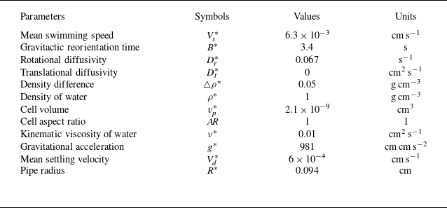
Relevant dimensional parameters used in this work, with the cell parameters corresponding to Chlamydomonas augustae, are primarily taken from Pedley & Kessler (Reference Pedley and Kessler1990) and Hwang & Pedley (Reference Hwang and Pedley2014a ,Reference Hwang and Pedley b ).

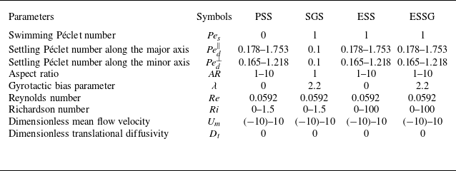
Ranges of relevant dimensionless parameters used in this work. While varying the aspect ratio of the particle, we keep the volume and the density of the particle constant, ensuring that the negative buoyant force of a single particle remains fixed.

The typical parameters of the model organisms Chlamydomonas augustae are used for SGS, as listed in table 1, with the non-dimensional parameters given in table 2. For comparison, we also consider PSS, ESS and ESSG, maintaining an identical particle volume to SGS but varying aspect ratios
 $A\!R$
between
 $1$
and
 $10$
.
3.1. The PSS and SGS
Neglecting the translational diffusion, Fung (Reference Fung2023) have provided the analytical solution for PSS and SGS:
 \begin{gather} f(r,\theta ,\phi )=\frac {C}{4\pi } \exp[\xi u(r)] \end{gather}
for PSS, and
 \begin{gather} f(r,\theta ,\phi )=C\exp[\xi u(r)]\, \frac {\lambda }{4\pi \sinh \lambda } \exp (\lambda \sin \theta \cos \phi ) \end{gather}
for SGS, where
 \begin{equation} \xi = \begin{cases} \displaystyle \frac {3\alpha _0}{{\textit {Pe}}_d^{\parallel }-{\textit {Pe}}_d^{\perp }} & \mbox { for PSS}, \\[12pt] \displaystyle \frac {\lambda }{2\,{\textit {Pe}}_s} & \mbox { for SGS}. \end{cases} \end{equation}
We denote
 $\xi$
as the distribution index hereinafter. In (3.1) and (3.2),
 $C$
represents the normalisation factor. It can be verified that both (3.1) and (3.2) satisfy the boundary conditions (2.27) for
 $f$
, but do not satisfy the boundary condition (2.28) for
 $\mathrm {d}f/\mathrm {d}r$
. However, since translational diffusion is neglected in both works, the zero-flux boundary condition at the wall is still satisfied by (3.1). By integrating over the orientational space, one obtains the same expression for radial particle concentration distribution for both PSS and SGS:
 \begin{gather} n(r)=C \exp\left [\xi u(r)\right ]. \end{gather}
Comparisons between (3.4) and the numerical solution of Wang et al. (Reference Wang, Jiang and Chen2023) are presented in Appendix B, demonstrating good agreement. Although (3.4) still depends on the flow velocity profile, it offers desirable efficiency in iterating the steady buoyancy–flow coupling problem.
Inspection of (3.4) reveals that the particle concentration scales exponentially with the local downward flow velocity. Therefore, within a downward discharge, the particle concentration around the centreline far exceeds the average concentration. With non-negligible buoyant force, this high concentration further drives an acceleration of the velocity around the centreline, which finally balances with the viscous force if the average particle concentration is not too high. The exponential dependence of particle concentration on the flow velocity profile, and the balance between the non-uniform buoyant force and the viscous force, explain some of the results presented in § 3.1.1, which have also been discussed in Wang et al. (Reference Wang, Jiang and Chen2023) and Fung (Reference Fung2023) for the downwelling scenario.
However, singularity (centreline concentration
 $n(0)$
approaches infinity) may arise when the average particle concentration exceeds a threshold, causing the viscous force to no longer sustain the buoyant force. This imbalance directs more particles into the centreline via a positive feedback loop, resulting in gyrotactic instability (Bees Reference Bees2020). As shown by Fung & Hwang (Reference Fung and Hwang2020) and Fung (Reference Fung2021) for a suspension subject to a downwelling discharge, a single steady plume is expected when
 $\mathrm {\textit {Ri}} \lt \mathrm {\textit {Ri}}_{\textit{s}} = 8/({\textit {Re}}\, \xi )$
. As
 $\mathrm {\textit {Ri}}$
exceeds
 $\mathrm {\textit {Ri}}_{\textit{s}}$
but remains smaller than a discharge-dependent critical value
 $\mathrm {\textit {Ri}}_{\textit {c}}$
, bifurcating solutions occur. A continued increase in
 $\mathrm {\textit {Ri}}$
suppresses the existence of steady solutions, leading to a blow-up until beyond the first transcritical point
 $\mathrm {\textit {Ri}}_{{c},1} = \kappa _{{c},1}^2/({\textit {Re}}\, \xi )$
, where
 $\kappa _{{c},1}$
is the first zero of the second Bessel function of the first kind
 $\mathrm {J}_2(r)$
. Therefore, to prevent the blow-up of the focused beam and avoid multiple branches of steady solutions in the downwelling flows, we restrict
 $\mathrm {\textit {Ri}}$
to be below the critical value
 $\mathrm {\textit {Ri}}_{\textit{s}}$
for a single steady solution. Since the distribution indices (
 $\xi = 83.4,53.8,5.5$
) of PSS are much higher than that of SGS (
 $\xi = 1.1$
), we use an upper limit
 $\mathrm {\textit {Ri}} = 1.5$
for comparison. This range of
 $\mathrm {\textit {Ri}}$
ensures a single steady solution in upwelling flows as well.
Fung (Reference Fung2021, chapter 5) has also indicated a maximum threshold for the discharge
 $Q$
at a given
 $\mathrm {\textit {Ri}}$
, beyond which the discharge is unachievable or singularity arises, with the concentration profile approaching a Dirac delta function. Based on this, we limit the mean downwelling flow velocity
 $U_m$
in the coupling cases to ensure that the centreline concentration
 $n(0)$
remains below a threshold
 $2000$
. Otherwise, the concentration profile is ill-posed in our method, and the volume fraction at the centreline exceeds the dilute limit
 $2.5\,\%$
. Furthermore, due to the strong shear near the wall, a sharp decrease of concentration is also expected, as described by (3.4) and observed numerically. In this scenario, the concentration profile also approaches a Dirac delta function, which cannot be well expanded using the basis functions. Although the concentration and velocity profile can be obtained with the analytical solution (3.4), the same issue arises when solving the Brenner scaler field
 $b(r,\theta ,\phi )$
(2.38). Therefore, we impose a lower limit on the mean upwelling flow velocity
 $U_m$
for each kind of particles by comparing the numerical and analytical concentration solutions. The lower limit is notably small for SGS, with distribution indices
 $\xi =83.4$
and
 $53.8$
.
3.1.1. Velocity and concentration profiles
The particle concentration profiles
 $n(r)$
of PSS and SGS at several mean flow velocities
 $U_m$
are presented in figure 2, followed by the flow velocity profiles
 $U(r)$
near the centreline corresponding to coupling cases in figure 3. With constant particle volume, the distribution index
 $\xi$
decreases as the aspect ratio
 $A\!R$
increases. Consequently, PSS with a smaller
 $A\!R$
, subjected to a stronger flow, are more concentrated around the centreline or at the wall, depending on the flow direction. On the other hand, SGS have a much smaller
 $\xi$
, leading to a relatively uniform distribution. To further illustrate the orientational-settling-induced accumulation of SGS and gyrotactic focusing of PSS, we plot the variations of the centreline particle concentration
 $n(0)$
and wall particle concentration
 $n(1)$
against
 $U_m$
in figures 4(a,b). As shown, there are notable increases in
 $n(0)$
and
 $n(1)$
with increasing
 $|U_m|$
.
Concentration profile
 $n(r)$
for PSS,
 $(A\!R, {\textit {Pe}}_d^{\parallel }, {\textit {Pe}}_d^{\perp })=(1.5,0.178,0.165), (2,0.264,0.230), (10,1.753,1.218)$
, and SGS,
 $({\textit {Pe}}_s,\lambda )=(1,2.2)$
.

When considering the buoyancy–flow coupling effect in a downwelling flow, the negative buoyant force decreases from the accumulation region around the centreline to the depletion region near the wall. As a result, the flow velocity increases around the pipe centreline and decreases near the wall, as shown in figures 3(a,b). The buoyancy–flow coupling effect is more pronounced for PSS with a smaller
 $A\!R$
due to more intensive accumulation around the centreline, as also evidenced in the right-hand half of figure 4(c). Additionally, a more noticeable buoyancy–flow coupling effect on the flow is observed for moderate
 $U_m$
in figure 4(c). This can be explained by examining the relative strength between the pressure gradient and the buoyant force, as described in (2.13). At high discharge, the uneven distribution of buoyancy does not notably deviate the flow velocity. However, it still leads to a significant enhancement of
 $n(0)$
compared to the non-coupling case (for instance,
 $n(0)$
increases nearly 20-fold for PSS with
 $A\!R = 1.5$
at
 $U_m = 0.6$
) , as shown in figure 4(a), because the radial concentration profile depends exponentially on the flow velocity profile.
For upwelling flow, we observe extremely limited modification on the particle concentration distribution (figures 2
c, 4
b) and flow velocity profile (figures 3
c, 4
c) by the buoyancy–flow coupling. Even with the same small mean flow velocities
 $U_m=\pm 0.1$
, the acceleration of the centreline flow velocity is comparatively negligible in upwelling flow. This is because the negative buoyant force, which is strongest at the wall, is less effective at driving the flow downwards compared to when it is strongest at the centreline in downwelling flow. As the upwelling discharge increases, both the no-slip wall effect and the pressure gradient quickly become dominant, causing the flow consequently to approach a Poiseuille profile with
 $U(0)/U_m = 2$
. As a result, the particle concentration profiles become indistinguishable from those of the non-coupling cases, as shown in figures 4(b,c).
Normalised flow velocity profile
 $U(r)/U_m$
for PSS,
 $(A\!R, {\textit {Pe}}_d^{\parallel }, {\textit {Pe}}_d^{\perp })=(1.5,0.178,0.165), (2,0.264,0.230), (10,1.753,1.218)$
, and SGS
 $({\textit {Pe}}_s,\lambda )=(1,2.2)$
, with buoyancy–flow coupling effect. Here,
 $\mathrm {\textit {Ri}}=1.5$
in all cases except for Poiseuille flows.

Variations of (a) centreline particle concentration
 $n(0)$
, (b) wall particle concentration
 $n(1)$
, and (c) normalised centreline flow velocity
 $U(0)/U_m$
, as functions of
 $U_m$
for PSS,
 $(A\!R, {\textit {Pe}}_d^{\parallel }, {\textit {Pe}}_d^{\perp })= (1.5,0.178,0.165), (2,0.264,0.230), (10,1.753,1.218)$
, and SGS,
 $({\textit {Pe}}_s,\lambda )=(1,2.2)$
. The crosses in (c) indicate ill-defined points where both
 $U(0)$
and
 $U_m$
are identically zero. The cu-toffs here indicate a maximum centreline particle volume fraction exceeding the dilute limit
 $2.5\,\%$
in the downwelling flows, as well as a sharp concentration gradient at the wall that is difficult to resolve using the Galerkin method.

3.1.2. Dispersion
The variations of drift velocity
 $U_d$
, dispersivity
 $D_{\mathrm {T}}$
, and time elapsed to steady dispersion
 $t_{\textit{s}}$
with
 $U_m$
are plotted in figure 5. In downwelling flows,
 $U_d$
of both PSS and SGS without coupling effect increases with
 $U_m$
and eventually scales with
 $2U_m$
, as the particles are primarily concentrated near the centreline. Downward settling and upward swimming separate different kinds of particles with small deviations. In upwelling flows, the contribution from upward advection diminishes as the discharge increases, and
 $U_d$
is almost entirely determined by settling or swimming. With the coupling effect, a slight increase of
 $U_d$
is observed in the downwelling flows for PSS with
 $A\!R=1.5$
and
 $2$
, as a result of more concentrated particles and accelerated centreline velocity. In upwelling flows, or for less concentrated particles, the buoyancy–flow coupling effect does not lead to any noticeable deviation of
 $U_d$
from the non-coupling cases.
For non-coupling cases in downwelling flows, the dispersivity
 $D_{\textit{T}}$
alternates between increasing and decreasing several times as
 $U_m$
, indicating a strong dependence of
 $D_{\textit{T}}$
on the interaction between flow shear, particle distribution, and their migration across the cross-section. This behaviour can be explained by the fact that flow shear itself influences both particle distribution and migration within the cross-section. On the one hand, an increase in
 $U_m$
enhances shear-induced dispersion if the particles are uniformly distributed across the cross-section. On the other hand, as
 $U_m$
increases, the concentration profile becomes more focused, causing the particles to sample nearly identical advective velocities, which consequently inhibits dispersion. These two opposing effects account for the initial increase and subsequent decrease in
 $D_{\mathrm {T}}$
observed in all non-coupling cases. We note that an additional increase of
 $D_{\textit{T}}$
appears for less elongated PSS (
 $U_m \in [2,4]$
for
 $A\!R=1.5$
, and
 $U_m\in [3,6.5]$
for
 $A\!R=2$
), which is possibly due to reduced cross-sectional migration ability in strong shear, favouring axial dispersion. The buoyancy–flow coupling effect results in a pronounced enhancement of
 $D_{\textit{T}}$
before the centreline concentration exceeds the dilute limitation. Although particles become much more concentrated around the centreline, the enhanced velocity gradient still increases the dispersivity, as shown in the inset of figure 5(b), where we compare the concentration and shear profiles near the centreline of coupling and non-coupling cases for
 $A\!R=2$
at
 $U_m=4$
. In upwelling flows, the variation of
 $D_{\textit{T}}$
follows a simple pattern: an initial increase followed by a decrease, demonstrating the sequential dominance of shear-induced dispersion followed by extreme wall accumulation.
Variations of (a) drift velocity
 $U_d$
, (b) dispersivity
 $D_{\mathrm {T}}$
(inset: comparison between the particle concentration profiles
 $n(r)$
and velocity gradient profiles
 $\mathrm {d}U/\mathrm {d}r$
near the centreline of coupling and non-coupling cases with
 $(A\!R,U_m)=(2,4)$
), and (c) time elapsed to steady dispersion
 $t_{\textit{s}}$
with
 $U_m$
for PSS,
 $(A\!R, {\textit {Pe}}_d^{\parallel }, {\textit {Pe}}_d^{\perp })= (1.5,0.178,0.165), (2,0.264,0.230), (10,1.753,1.218)$
, and SGS,
 $({\textit {Pe}}_s,{\textit {Pe}}_d,\lambda )=(1,0.1,2.2)$
. The cut-offs here indicate a maximum centreline particle volume fraction exceeding the dilute limit
 $2.5\,\%$
in the downwelling flows, as well as a sharp concentration gradient at the wall that is difficult to resolve using the Galerkin method.

Next, we discuss the time elapsed to steady dispersion,
 $t_{\textit{s}}$
, as shown in figure 5(c). First, we find that
 $t_{\textit{s}}$
for PSS is larger than that for SGS, which is most pronounced for those less elongated PSS. Since
 $t_{\textit{s}}$
measures how quickly particles fully sample the radius–orientation space, this difference is primarily due to the different streamline-crossing abilities of PSS and SGS. For PSS, the radial migration is subdominant to the downward settling, regardless of orientation. In contrast, SGS simply swim along their current orientation. Therefore, the radial migration ability of PSS is less effective compared to SGS, which explains the longer
 $t_{\textit{s}}$
for the PSS. Another observation is that as
 $U_m$
increases,
 $t_{\textit{s}}$
for SGS increases monotonically, while
 $t_{\textit{s}}$
of PSS decreases initially, and increases or saturates subsequently. This indicates a trade-off between swimming/slipping with rotational noise and with shear-induced rotation. Comparing with no flow, a small discharge enables effective sampling in both the orientational space and cross-section for PSS, but leads to reduced cross-sectional migration of active particles as their diffusive trajectories due to noisy swimming are overwhelmed by the deterministic shear-induced rotation. At high discharges,
 $t_{\textit{s}}$
of PSS and SGS saturates or slightly increases due to a more focused final concentration profile accompanied by reduced cross-sectional migration.
3.2. The ESS
In § 3.1, we observed that PSS exhibit a concentration distribution similar to SGS in response to the background flow, focusing around the centreline in downwelling flow, and migrating to the wall in upwelling flow, respectively. We now further investigate the synergetic effect of orientation-dependent settling and swimming. This phenomenon is common among many chain-forming micro-algae due to their elongated shape (Sohn et al. Reference Sohn, Seo, Choi, Lee, Kang and Kang2011; Lovecchio et al. Reference Lovecchio, Climent, Stocker and Durham2019; Bearon & Durham Reference Bearon and Durham2023) and a density
 $5$
–
 $10\,\%$
higher than the surrounding aqueous medium (Kamykowski, Reed & Kirkpatrick Reference Kamykowski, Reed and Kirkpatrick1992).
The simpler scenario of elongated non-settling swimmers (ENSS) reminds us of the shear-induced trapping in a planar Poiseuille flow (Rusconi et al. Reference Rusconi, Guasto and Stocker2014; Barry et al. Reference Barry, Rusconi, Guasto and Stocker2015). In such flows, below a critical mean shear rate, the cross-sectional concentration profile of ENSS exhibits high-shear trapping, characterised by a concentration peak at regions of strong shear. As the mean shear rate increases beyond the threshold, the profile transitions to low-shear trapping, with the concentration peak shifting towards the near-centreline region, where the shear is relatively weaker.
It is worth noting that previous theoretical studies on shear-induced trapping were conducted predominantly within a planar Poiseuille flow with periodic boundary conditions to avoid specifying detailed boundary interactions (Rusconi et al. Reference Rusconi, Guasto and Stocker2014; Vennamneni et al. Reference Vennamneni, Nambiar and Subramanian2020; Maretvadakethope et al. Reference Maretvadakethope, Hazel, Vasiev and Bearon2023). Alternatively, Bearon & Hazel (Reference Bearon and Hazel2015) employed a Robin-type boundary condition but observed the formation of a concentration boundary layer. Experimental investigations, on the other hand, often focused on particle concentrations within the central portion of the channel cross-section to minimise wall effects. For instance, the experiments by Rusconi et al. (Reference Rusconi, Guasto and Stocker2014) and Barry et al. (Reference Barry, Rusconi, Guasto and Stocker2015) measured concentrations only within the central
 $60\,\%$
and
 $70\,\%$
of the cross-section, respectively.
Periodic boundary conditions, commonly used in previous theoretical studies, are not applicable to a circular pipe configuration due to the transition from reflective symmetry in planar flows to rotational symmetry in cylindrical flows. Therefore, reflection boundary conditions are used in this work. This raises the question of how the findings from planar two-dimensional configurations compare to those from the cylindrical three-dimensional configuration used here, given the differing boundary conditions. This question is analysed from two aspects. First, the reflection boundary conditions in this work inevitably combine the effects of wall reflection (a sudden inversion of wall-normal swimming direction component) and high-shear trapping near the wall, where shear is strongest. This is evidenced by a reduced wall concentration for less elongated particles as will be seen in figure 6 and similar findings reported by Maretvadakethope et al. (Reference Maretvadakethope, Hazel, Vasiev and Bearon2023, figure 4). Second, while high-shear trapping near the wall occurs at low discharges, the low-shear trapping near the centreline at high discharges is less influenced by particle–wall interactions. At high discharges, most swimmers are located far from the wall, and their rapid rotation is governed primarily by strong shear rather than boundary effects at the wall (Ezhilan & Saintillan Reference Ezhilan and Saintillan2015; Wang et al. Reference Wang, Jiang and Chen2022). For instance, figure 4 of Maretvadakethope et al. (Reference Maretvadakethope, Hazel, Vasiev and Bearon2023) directly compared the cross-sectional distributions of elongated swimmers in a double inverse Poiseuille flow with periodic boundary conditions, and a single Poiseuille flow with reflection boundary conditions. Their findings confirmed that reflection boundary conditions have only minimal impact on the distribution near the wall, and do not notably influence low-shear trapping at high discharges. Consequently, we anticipate that the reflection boundary conditions employed in this work do not affect the qualitative analysis of low-shear trapping for elongated swimmers.
Concentration profile
 $n(r)$
for ESS,
 $(A\!R, {\textit {Pe}}_d^{\parallel }, {\textit {Pe}}_d^{\perp })= (1.5,0.178,0.165), (2,0.264,0.230), (10,1.753,1.218)$
, and ENSS,
 ${\textit {Pe}}_d^{\parallel }={\textit {Pe}}_d^{\perp }=0$
. Here,
 ${\textit {Pe}}_s=1$
in all cases.

Given the weaker aggregation intensity of ESS compared to PSS, we adopt a reasonably large Richardson number,
 $\mathrm {\textit {Ri}} = 100$
. This corresponds to an average volume fraction of
 $0.086\,\%$
, which is well below the dilute suspension threshold of
 $2.5\,\%$
– a limit beyond which particle interactions can no longer be neglected (Ishikawa & Pedley Reference Ishikawa and Pedley2007). The choice of a larger Richardson number is intended to enhance the contrast between cases with buoyancy–flow coupling and those without.
3.2.1. Velocity and concentration profiles
Particle concentration profiles
 $n(r)$
and flow velocity profiles
 $U(r)$
for ESS under several mean flow velocities
 $U_m$
are shown in figures 6 and 7, respectively. Comparisons with non-coupling and non-settling cases are also included. We quantify the accumulation of particles by calculating the mean radial position
 $r_m \triangleq \int _0^{1} 2 r^2 n \,\mathrm {d}r$
and mean square displacement of the radial position
 $\sigma _r^2 \triangleq \int _0^{1} 2(r-r_m)^2 r n\,\mathrm {d}r$
. Additionally, we measure the modification of buoyancy on the flow by
 $U(0)/U_m$
. These quantities are plotted against
 $U_m$
in figure 8.
Normalised flow velocity profile
 $U(r)/U_m$
for ESS,
 $(A\!R, {\textit {Pe}}_d^{\parallel }, {\textit {Pe}}_d^{\perp })=(1.5,0.178,0.165), (2,0.264,0.230), (10,1.753,1.218)$
, with buoyancy–flow coupling effect. Here,
 $\mathrm {\textit {Ri}}=100$
in all cases except for Poiseuille flows.

Less elongated swimmers (
 $A\!R=1.5,2$
), regardless of whether they are settling, non-settling, and with or without coupling, exhibit a concentration bump (
 $\simeq 1.4$
for
 $U_m=10$
) near the wall. This bump is positively correlated to
 $A\!R$
and
 $U_m$
. Since this near-wall concentration peak exists for coupling, settling and non-settling cases, it is reasonable to conclude that the elongation of the swimmers results in such near-wall concentration peak. The nearly identical distributions for settling and non-settling cases, as well as for both flow directions, indicate that high-shear trapping dominates orientation-dependent settling, which typically drives centreline focusing. However, ESS with
 $A\!R=10$
behave markedly differently compared to those non-settling and less elongated particles. In weak to moderate downwelling flow (
 $U_m=0.1,1$
), orientation-dependent settling results in a local depletion zone where non-settling counterparts typically accumulate. This bimodal distribution arises from dual accumulation mechanisms: elongation-induced accumulation near the wall, inherited from high-shear trapping, and orientational-settling-induced focusing around the centreline, resembling that observed in PSS. For PSS, increasing
 $A\!R$
leads to a smaller distribution index
 $\xi$
if the particle volume is kept constant, as the settling velocity difference
 ${\textit {Pe}}_d^{\parallel }-{\textit {Pe}}_d^{\perp }$
becomes larger (see (3.3)). For ESS, however, only when
 $A\!R=10$
do the settling Péclet numbers,
 ${\textit {Pe}}_d^{\parallel }$
and
 ${\textit {Pe}}_d^{\perp }$
, become comparable with
 ${\textit {Pe}}_s$
, resulting in a concentration distribution that is distinct from the non-settling case. In the strongest downwelling flow (
 $U_m=10$
), the bimodal distribution is replaced by a single concentration peak away from the wall (
 $r\simeq 0.4$
). In contrast, the concentration peak of the non-settling cases shifts closer to the wall. For upwelling flow, the dual accumulation mechanisms work synergistically, consistently producing a single, enhanced concentration peak near the wall.
Since the non-trivial transition from high-shear trapping to low-shear of elongated swimmers suspended in a planar Poiseuille flow with increasing discharge has been well investigated, here we find that such a low-shear trapping pattern does not occur in a circular pipe configuration. As shown in figures 6 and 8(a), highly elongated non-settling swimmers (
 $A\!R=10$
) move closer to the wall (
 $r_m$
increases) with increasing discharge, while less elongated swimmers (
 $A\!R=1.5, 2$
) remain nearly stationary on average (
 $r_m$
saturates). This shift is accompanied by more intensive accumulation for highly elongated swimmers (
 $A\!R=10$
), or unchanged accumulation for less elongated swimmers (
 $A\!R=1.5, 2$
), irrespective of the flow direction, as shown in figure 8(b). These observations highlight a fundamental difference in how the cross-sectional concentration distribution responds to flow strength in planar Poiseuille flow versus pipe flow. Specifically, the low-shear trapping observed in strong planar Poiseuille flows is absent in strong pipe flows. This difference can be attributed to the contrasting trajectories of swimmers in the two flow types. In planar Poiseuille flows, deterministic elongated swimmers exhibit two primary types of periodic trajectories, depending on the initial condition: swinging (where the swimmer crosses the centreline) and tumbling (where the swimmer does not cross the centreline) (Zöttl & Stark Reference Zöttl and Stark2012, Reference Zöttl and Stark2013; Zöttl Reference Zöttl2014). The transition of high-shear trapping to low-shear trapping in planar Poiseuille flows can thus be interpreted as a competition between these two trajectory types. In contrast, deterministic elongated swimmers in pipe flows exhibit helical-like swinging (the azimuthal angle
 $\phi$
cannot traverse from
 $0$
to
 $2\pi$
) and tumbling (
 $\phi$
can traverse from
 $0$
to
 $2\pi$
), both of which do not cross the centreline (Zöttl & Stark Reference Zöttl and Stark2012, Reference Zöttl and Stark2013; Zöttl Reference Zöttl2014), thus reducing the probability of finding a swimmer around the pipe centreline. The results in figure 8 confirm that low-shear trapping is unlikely to occur in circular configurations for ENSS.
Nonetheless, we observe a non-trivial variation of radial concentration distribution with the
 $U_m$
for ESS with
 $A\!R=10$
in strong downwelling flows, as shown in figures 6(c) and 8(a,b). The ESS with
 $A\!R=10$
exhibit an intensified peak concentration moving towards the centreline (
 $r_m$
decreases) as
 $U_m$
exceeds approximately
 $2$
, which is akin to low-shear trapping pattern in planar Poiseuille flow. In contrast, in upwelling flows, this phenomenon does not occur but is replaced by a more focused concentration profile near the wall due to a change of sign of the flow velocity gradient. Therefore, although the low-shear trapping pattern previously found in the case of ENSS subjected to a planar Poiseuille flow does not appear in a circular pipe flow, the inclusion of orientation-dependent settling velocity could instead assist in forming such a distribution pattern.
The effect of buoyancy–flow coupling is more complicated, depending on
 $A\!R$
, settling and flow direction. For both flow directions, less elongated settling swimmers (
 $A\!R=1.5,2$
) consistently accumulate near the wall, resulting in a negative buoyancy profile that attenuates from the wall to the centreline. This leads to weak decreases and increases in central velocity in downwelling and upwelling flows, respectively, as shown in figures 7 and 8(c). The non-trivial response of very elongated settling swimmers (
 $A\!R=10$
) to increasing downwelling discharge also extends to their buoyancy–flow coupling effect. As shown in figures 7(a–c) and 8(c), the centreline velocity experiences enhancement (
 $U(0)/U_m \gt 2$
), reduction (
 $U(0)/U_m \lt 2$
), and finally again enhancement, due to the competition between high-shear trapping and orientational-settling-induced focusing. It is noteworthy that as the accumulation intensity for ESS is relatively weak, with the maximum concentration of the order of
 $O(10)$
, the buoyancy–flow coupling effect only causes the normalised centreline flow velocity to deviate from 2 by an order of
 $O(0.01)$
, and the concentration profiles of coupling and non-coupling cases are very close.
Variations of (a) mean radial position
 $r_m$
, (b) mean square displacement of the radial position
 $\sigma _r^2$
, and (c) normalised centreline flow velocity
 $U(0)/U_m$
as functions of
 $U_m$
for ESS,
 $(A\!R, {\textit {Pe}}_d^{\parallel }, {\textit {Pe}}_d^{\perp })=(1.5,0.178,0.165), (2,0.264,0.230), (10,1.753,1.218)$
, and ENSS,
 ${\textit {Pe}}_d^{\parallel }={\textit {Pe}}_d^{\perp }=0$
. Here,
 ${\textit {Pe}}_s=1$
in all cases. The crosses in (c) indicate ill-defined points where both
 $U(0)$
and
 $U_m$
are identically zero.

3.2.2. Dispersion
The variations of drift velocity
 $U_d$
, dispersivity
 $D_{\textit{T}}$
, and time elapsed to steady dispersion
 $t_{\textit{s}}$
for both elongated settling and non-settling swimmers are plotted against
 $U_m$
in figure 9. Cases with buoyancy–flow coupling are also presented.
Variations of (a) drift velocity
 $U_d$
, (b) dispersivity
 $D_{\mathrm {T}}$
, and (c) time elapsed to steady dispersion
 $t_{\textit{s}}$
as functions of
 $U_m$
for ESS,
 $(A\!R, {\textit {Pe}}_d^{\parallel }, {\textit {Pe}}_d^{\perp })=(1.5,0.178,0.165), (2,0.264,0.230), (10,1.753,1.218)$
, and ENSS,
 ${\textit {Pe}}_d^{\parallel }={\textit {Pe}}_d^{\perp }=0$
. Here,
 ${\textit {Pe}}_s=1$
in all cases.

Since elongation of non-settling swimmers enhances near-wall accumulation irrespective of the flow direction, non-settling swimmers with a larger
 $A\!R$
drift more slowly compared to those with a smaller
 $A\!R$
. In upwelling flows, settling results in a more wall-accumulated concentration profile (figures 8
a,b), and therefore a smaller advective velocity. Meanwhile, sedimentation itself also contributes to the drift velocity in the opposite direction of the flow. The combination of these two effects explains the decreased magnitude of
 $U_d$
in upwelling flows for settling swimmers. In downwelling flows, the opposite process occurs, and ESS drift faster than their non-settling counterparts. For both flow directions, swimmers with
 $A\!R = 10$
show the most pronounced differences between settling and non-settling cases. The buoyancy–flow coupling only slightly increases
 $U_d$
for swimmers with
 $A\!R=10$
, as there are limited modifications in concentration and velocity in other situations, as shown in figure 8.
Since elongation always enhances the accumulation of swimmers (see figure 8
b), the dispersivity
 $D_{\textit{T}}$
of swimmers with a larger
 $A\!R$
is hindered more intensively, as shown in figure 9(b). For non-settling swimmers,
 $D_{\textit{T}}$
is symmetrically distributed on both sides of
 $U_m=0$
. When settling is included,
 $D_{\textit{T}}$
increases in downwelling flows due to the profile spreading out but decreases in upwelling flows as the profile becomes more concentrated (figure 8
b), which is particularly notable for
 $A\!R=10$
. The buoyancy–flow coupling has a more pronounced impact on
 $D_{\textit{T}}$
at relatively strong flows (
 $|U_m| \gt 5$
), where
 $D_{\textit{T}}$
may be either enhanced or suppressed depending on the flow direction and
 $A\!R$
, due to subtle variations in both the concentration distribution and velocity profile.
As shown in figure 9(c), a larger discharge increases
 $t_{\textit{s}}$
in all cases, indicating a reduced radial migration ability of elongated swimmers, which contrasts with PSS as observed in figure 5(c). We also see that elongation decreases
 $t_{\textit{s}}$
, possibly due to the effective radial migration of elongated swimmers being enhanced by a stronger shear alignment. The effects of settling and buoyancy–flow coupling on
 $t_{\textit{s}}$
are non-monotonic and resist intuitive interpretation. However, it is noteworthy that the variations between
 $D_{\textit{T}}$
and
 $t_{\textit{s}}$
remain consistent, regardless of changes in
 $U_m$
, the presence or absence of settling, or the inclusion of the buoyancy–flow coupling effect.
3.3. ESSG
As PSS and SGS exhibit similar focusing towards the centreline in downwelling flow, and migration towards the wall in upwelling flow, respectively, it raises the question of how particles would behave when both effects are present. This subsection investigates the behaviour of ESSG under these combined effects.
3.3.1. Velocity and concentration profiles
The particle concentration profiles for both downwelling and upwelling flows are shown in figure 10, comparing cases with coupling (
 $\mathrm {\textit {Ri}}=100$
), without coupling (
 $\mathrm {\textit {Ri}}=0$
), and non-settling. This is followed by the normalised flow velocity profiles presented in figure 11.
For
 $\mathrm {\textit {Ri}}=0$
, elongation weakens the gyrotactic focusing both around the centreline and at the wall (see also figures 12
a,b), in line with findings from previous studies on vertical channel flows (Bearon, Hazel & Thorn Reference Bearon, Hazel and Thorn2011; Croze et al. Reference Croze, Sardina, Ahmed, Bees and Brandt2013). For extremely elongated swimmers (
 $A\!R=10$
), the concentration peak shifts away from the centreline or the wall to an intermediate radial position (
 $U_m = -0.1,-1,\pm 10$
). Thus elongation influences particle behaviour differently depending on the presence of gyrotaxis: for non-settling, non-gyrotactic swimmers, elongation enhances accumulation in the near-wall, high-shear region. In contrast, for non-settling gyrotactic swimmers, elongation negatively impacts the gyrotaxis-induced accumulation, affecting both centreline focusing in downwelling flows and wall accumulation in upwelling flows.
The inclusion of orientation-dependent settling velocity has minimal impact on the particle concentration profile except for improving centreline focusing in downwelling flows and wall accumulation in upwelling flows when
 $A\!R=10$
, which is in stark contrast to its marked effect observed in the absence of gyrotaxis.
For less elongated swimmers (
 $A\!R=1, 1.5, 2$
), the buoyancy–flow coupling effect creates more noticeable concentration differences and flow deviations compared to the non-coupling case, as seen in figures 10 and 11. For extremely elongated swimmers (
 $A\!R=10$
), the difference in concentration profile gradually diminishes when the downwelling flow gets strong, but the difference in flow velocity profile decays slower than those of less elongated swimmers in upwelling flow. Both of these treads can be attributed to elongation broadening the radial concentration distribution: a relatively uniform distribution in strong downwelling flow results in the weakest buoyancy–flow coupling effect (figure 11
c), while a concentration peak at a finite distance away from the wall can somewhat avoid the complete dominance of the no-slip condition (figure 11
f).
Concentration profile
 $n(r)$
for ESSG,
 $(A\!R, {\textit {Pe}}_d^{\parallel }, {\textit {Pe}}_d^{\perp })=(1.5,0.178,0.165), (2,0.264, 0.230), (10,1.753,1.218)$
, and ENSSG (elongated non-settling swimmers with gyrotaxis),
 ${\textit {Pe}}_d^{\parallel }={\textit {Pe}}_d^{\perp }=0$
. Here,
 ${\textit {Pe}}_s=1$
and
 $\lambda =2.2$
in all cases.

Normalised flow velocity profile
 $U(r)/U_m$
for ESSG,
 $(A\!R, {\textit {Pe}}_d^{\parallel }, {\textit {Pe}}_d^{\perp })=(1.5,0.178,0.165), (2,0.264,0.230), (10,1.753,1.218)$
, with buoyancy–flow coupling effect. Here,
 ${\textit {Pe}}_s=1$
,
 $\lambda =2$
and
 $\mathrm {\textit {Ri}}=100$
in all cases except for Poiseuille flows.

Variations of (a) mean radial position
 $r_m$
, (b) mean square displacement of the radial position
 $\sigma _r^2$
, and (c) normalised centreline flow velocity
 $U(0)/U_m$
as functions of
 $U_m$
for ESSG,
 $(A\!R, {\textit {Pe}}_d^{\parallel }, {\textit {Pe}}_d^{\perp })=(1,0.1,0.1), (1.5,0.178,0.165), (2,0.264,0.230), (10,1.753,1.218)$
, and ENSSG,
 ${\textit {Pe}}_d^{\parallel }={\textit {Pe}}_d^{\perp }=0$
. Here,
 ${\textit {Pe}}_s=1$
and
 $\lambda =2$
in all cases. The crosses in (c) indicate ill-defined points where both
 $U(0)$
and
 $U_m$
are identically zero.

3.3.2. Dispersion
The variations of drift velocity
 $U_d$
, dispersivity
 $D_{\mathrm {T}}$
and time elapsed to steady dispersion
 $t_{\textit{s}}$
with
 $U_m$
are plotted against
 $U_m$
in figure 13. Without settling, due to their more uniform distribution, elongated gyrotactic swimmers exhibit smaller
 $U_d$
in downwelling flows, and larger
 $U_d$
(in magnitude) in upwelling flows, compared to relatively spherical ones. The impact of orientation-dependent settling on the concentration distribution is negligible for less elongated swimmers (
 $A\!R\lt 10$
). Therefore, the difference in drift velocity between the settling and the non-settling conditions is caused only by the settling itself. This difference amplifies for the most elongated swimmers (
 $A\!R=10$
), as they are more concentrated and have larger settling speeds. When buoyancy–flow coupling is considered in downwelling flows,
 $U_d$
of relatively spherical gyrotactic swimmers exhibits a larger enhancement due to a more pronounced accelerated centreline velocity. In comparison,
 $U_d$
in upwelling flows is almost unaffected by the buoyancy–flow coupling effect.
The variations of
 $D_{\textit{T}}$
basically follow the same rules as discussed in § 3.1.2, except for the additional enhancement on
 $D_{\textit{T}}$
due to a more uniform concentration distribution for elongated swimmers. The effect of orientation-dependent settling intensifies with
 $A\!R$
, and is most notable for
 $A\!R=10$
. The
 $D_{\textit{T}}$
value of non-settling swimmers exhibits a consistent increasing trend, qualitatively different from that of settling swimmers with a saturating trend. This difference is again attributed to the intricate interplay between elongation and settling; as shown in figures 12(a,b), although non-settling swimmers with
 $A\!R=10$
are also guided towards the centreline or the wall in respective flow directions and become more concentrated, their decrease of
 $\sigma _r^2$
is notably slower. For the buoyancy–flow coupling effect, it results in an enhanced
 $D_{\textit{T}}$
in downwelling flows compared to non-coupling cases due to increased shear in the region around the centreline, as also discussed in § 3.1.2.
Finally, for the variation of the time elapsed to steady dispersion
 $t_{\textit{s}}$
with
 $U_m$
, we see a consistent trend with
 $D_{\textit{T}}$
, in line with § 3.1.2. Specifically, like
 $D_{\textit{T}}$
,
 $t_{\textit{s}}$
is enhanced by both elongation and buoyancy–flow coupling, whereas orientation-dependent settling is crucial only to the most elongated swimmers (
 $A\!R=10$
).
Variations of (a) drift velocity
 $U_d$
, (b) dispersivity
 $D_{\mathrm {T}}$
, and (c) time elapsed to steady dispersion
 $t_{\textit{s}}$
as functions of
 $U_m$
for ESSG,
 $(A\!R, {\textit {Pe}}_d^{\parallel }, {\textit {Pe}}_d^{\perp })=(1,0.1,0.1), (1.5,0.178,0.165), (2,0.264,0.230), (10,1.753, 1.218)$
, and ENSSG,
 ${\textit {Pe}}_d^{\parallel }={\textit {Pe}}_d^{\perp }=0$
. Here,
 ${\textit {Pe}}_s=1$
and
 $\lambda =2$
in all cases.

4. Concluding remarks
This study explores the buoyancy–flow coupled dispersion of passive and active spheroids in a vertical pipe with varying discharge. We first analysed PSS and SGS, noting that their concentration and flow velocity distributions can be similarly treated analytically (Fung Reference Fung2023). However, differences arise primarily in (i) the drift velocity of PSS, which can be upwards for small downwelling discharges due to gyrotaxis-induced up-swimming, and (ii) the dispersivity and time elapsed to steady dispersion, which exhibit qualitatively different trends due to contrasting streamline-crossing mechanisms. The PSS with less elongated shapes are characterised by extremely concentrated distribution. Therefore, the buoyancy–flow coupling effect notably modifies the flow velocity profile at small to moderate downwelling discharges, leading to enhanced dispersivity by increasing the mean shear rate where the particles accumulate.
We then moved to investigate ENSS, and found that elongation leads to accumulation in high-shear regions, a phenomenon parallel to high-shear trapping observed in planar Poiseuille flows. This accumulation is enhanced by both increased elongation and larger discharges. However, the low-shear trapping of non-settling elongated swimmers around the centreline, previously found in planar Poiseuille flows, does not occur in circular pipe flows. Instead, we found that the orientation-dependent settling velocity plays a similar role at high downwelling discharges: more elongated swimmers are guided by the settling velocity to the low-shear region. This results in notably enhanced drift velocity, as well as reduced dispersivity and time elapsed to steady dispersion.
Finally, we considered the combined effects of gyrotactic swimming and orientation-dependent settling, finding that their combined effect leads to a more uniform concentration profile. This is somewhat unexpected, as both gyrotactic swimming and orientation-dependent settling independently enhance accumulation. We attribute this phenomenon to the predominance of weakening effect of elongation on gyrotactic focusing, as ENSSG are more uniformly distributed than their ESSG counterparts. The strength of buoyancy–flow coupling is therefore reduced for ESSG compared with SSG, but the dispersivity and time elapsed to steady dispersion are largely enhanced.
The above findings highlight the complex effects of elongation and orientation-dependent settling on concentration distribution, flow velocity distribution, and dispersion in dilute suspensions of passive and active spheroids. The absence of low-shear trapping of ENSS in a circular pipe configuration and the similar low-shear trapping of ESS resulting from orientational-dependent settling are central observations. The disappearance of low-shear trapping typically found for ENSS is likely attributed to the rotational symmetry of the circular pipe configuration, which also substantially alters the periodic motions of ENSS, as found in previous works (Zöttl Reference Zöttl2014). The newly identified low-shear trapping exclusive to ESS and the gyrotaxis-like accumulation of PSS share a common physical origin. As described by Koch & Shaqfeh (Reference Koch and Shaqfeh1989), the orientational probability of elongated particles with rotational noises under shear flow increases in two extensional quadrants (the quadrants where the projection of the particle’s orientation onto the shear plane falls within angle
 $\pi /4$
from the axis of extension for the extensional component of the shear field). In downwelling flows, the radial component of the settling velocity of particles with orientations within the extensional quadrants always points to the centreline, while the opposite holds for upwelling flows. This allows orientation-dependent settling to either compete or cooperate with the directed swimming, depending on the flow direction.
Funding
This work is supported by Beijing Jianghe Water Resources Development Foundation (grant no. JHQB202228), the IWHR Research and Development Support Program (grant nos HY0199A112021 and WE90022307), and the Independent Research Project of State Key Laboratory of Water Cycle and Water Security in River Basin (grant no. SKL2024TS12).
Declaration of interests
The authors report no conflict of interest.
Appendix A. Detailed formulas for settling speeds
In the low-Reynolds-number limit, for a spheroid with aspect ratio
 $A\!R$
, equatorial radius
 $a^{\ast }$
and density
 $\rho ^{\ast } + \triangle \rho ^{\ast }$
suspended in a fluid with density
 $\rho ^{\ast }$
and kinetic viscosity
 $\nu ^{\ast }$
, the settling speeds along the major and minor axes can be calculated analytically as (Kim et al. Reference Kim, Karrila and Brenner1991)
 \begin{gather} V_{\parallel }^{\ast } = \frac {2}{9}\, \frac {\triangle \rho ^{\ast }\, g^{\ast } (a^{\ast })^2 A\!R}{\mu ^{\ast }}\, X(A\!R), \end{gather}
 \begin{gather} V_{\perp }^{\ast } = \frac {2}{9}\, \frac {\triangle \rho ^{\ast }\, g^{\ast } (a^{\ast })^2 A\!R}{\mu ^{\ast }}\, Y(A\!R), \end{gather}
where
 $X(A\!R)$
and
 $Y(A\!R)$
take the forms
 \begin{gather} X(A\!R) = (A\!R X^A)^{-1}, \end{gather}
 \begin{gather} Y(A\!R) =(A\!R Y^A)^{-1}. \end{gather}
Here,
 $X^A$
and
 $Y^A$
are calculated as
 \begin{gather} X^A = \tfrac {8}{3}e^3[-2e + (1+e^2) L]^{-1}, \end{gather}
 \begin{gather} Y^A = \tfrac {16}{3}e^3[2e+(3e^2-1)L]^{-1}, \end{gather}
where
 \begin{gather} e = \sqrt {1-\frac {1}{A\!R^2}}, \end{gather}
 \begin{gather} L = \ln \left (\frac {1+e}{1-e}\right ). \end{gather}
Appendix B. Comparison with analytical solution for PSS and SGS
Figure 14 is the comparison between our results and the analytical solution of Fung (Reference Fung2023) vertical pipe in Poiseuille flows. Perfect agreement is demonstrated.
Comparison between particle concentration profiles obtained by this work and the analytical solutions of Fung (Reference Fung2023). The background flow is set to be vertical pipe Poiseuille flows with
 $U_m=\pm 1$
. Here, (
 $A\!R, {\textit {Pe}}_d^{\parallel }, {\textit {Pe}}_d^{\perp }) = (10,1.753,1.218)$
for PSS, (
 ${\textit {Pe}}_s, \lambda ) = (1,2.2)$
for SGS.