


Impact Statement
Coral reef islands are vulnerable to climate change, not only from sea level rise, but also from seasonal and inter-annual climate forcings such as the Indian Monsoon and the Indian Ocean Dipole. However, systematic monitoring remains rare in Small Island Developing States such as the Maldives. We have developed a scalable, satellite-based framework using Sentinel-2 and Landsat to detect and model seasonal coastal changes across an entire Maldivian atoll. By disentangling sub-annual, inter-annual, and abrupt signals of change, we reveal how islands respond to weather and ocean conditions and how these shape coastal dynamics. These results help identify the most variable islands and assist policymakers and marine infrastructure planners in designing adaptation strategies based on spatial and temporal data.
1. Introduction
Coral reef islands are low-lying landforms that are particularly vulnerable to sea level rise (SLR) and climate-driven changes in oceanographic conditions. Understanding their morphological dynamics is critical for assessing their long-term habitability and informing coastal adaptation strategies. Coral reef islands are formed from unconsolidated accumulations of sediment originating from organic and inorganic material, primarily from the breakdown of coral and other marine organisms. Morphological response and coastal changes of these islands are driven by various environmental factors acting over different timescales, such as wave action, tidal currents, storms and SLR (e.g., Webb and Kench, Reference Webb and Kench2010; Ford, Reference Ford2013; Yates et al., Reference Yates, Cozannet, Garcin, Salaï and Walker2013; Ford and Kench, Reference Ford and Kench2015; Mann et al., Reference Mann, Bayliss-Smith and Westphal2016; Purkis et al., Reference Purkis, Gardiner, Johnston and Sheppard2016; Aslam and Kench, Reference Aslam and Kench2017; Duvat, Reference Duvat2019; Dawson, Reference Dawson2021; Sengupta et al., Reference Sengupta, Ford and Kench2021; Wu et al., Reference Wu, Duvat and Purkis2021; Rankey et al., Reference Rankey, Uriam and Perez2023; Menon et al., Reference Menon, Khanna, Misra and Jorry2024). These drivers are expected to vary due to climate change (e.g., Tebaldi et al., Reference Tebaldi, Ranasinghe, Vousdoukas, Rasmussen, Vega-Westhoff, Kirezci, Kopp, Sriver and Mentaschi2021; Shivamurthy et al., Reference Shivamurthy, Narendr and Aithal2022). Local, regional, and global drivers of coastal changes (Melet et al., Reference Melet, Teatini, Le Cozannet, Jamet, Conversi, Benveniste and Almar2020) must be identified and monitored to manage natural resources and development effectively on such islands and to devise sustainable strategies for mitigating erosion, flooding, submergence, and habitat loss to ensure the resilience and persistence of coastal ecosystems and communities.
SLR is a significant driver of coastal erosion on multi-decadal timescales. However, SLR alone does not sufficiently explain the high erosion rates observed in certain regions, including those experiencing relatively rapid sea-level increases (e.g., Ford and Kench, Reference Ford and Kench2015; Aslam and Kench, Reference Aslam and Kench2017). Recent evidence suggests that coral reef islands demonstrate greater geomorphic resilience than previously assumed, responding to SLR through vertical accretion and lateral expansion (e.g., Masselink et al., Reference Masselink, McCall, Beetham, Kench and Storlazzi2021). These adaptive processes support projections that many reef islands may remain physically viable and potentially inhabitable through the 21st century (e.g., Ford and Kench, Reference Ford and Kench2015; McLean and Kench, Reference McLean and Kench2015; Kench et al., Reference Kench, Liang, Ford, Owen, Aslam, Ryan, Turner, Beetham, Dickson, Stephenson, Vila-Concejo and McLean2023). Nonetheless, other studies indicate that SLR poses significant risks, including saline intrusion into freshwater lenses, increased flooding frequency, shoreline retreat, potential submergence, and associated pressures for population displacement or migration (e.g., Charan et al., Reference Charan, Kaur, Singh and Leal Filho2017; Storlazzi et al., Reference Storlazzi, Gingerich, van, Cheriton, Swarzenski, Quataert, Voss, Field, Annamalai, Piniak and McCall2018).
Coastal ecosystems, namely coral reefs, mangroves, and seagrass beds, act as natural barriers against wave action, thus mitigating erosion (e.g., Bramante et al., Reference Bramante, Ashton, Storlazzi, Cheriton and Donnelly2020). These ecosystems also supply the sediments that constitute the islands (e.g., Perry et al., Reference Perry, Kench, O’Leary, Morgan and Januchowski-Hartley2015; Tuck et al., Reference Tuck, Ford, Kench and Masselink2021). Climate change and human activities play a key role in the health and persistence of these ecosystems (Hoegh-Guldberg et al., Reference Hoegh-Guldberg, Mumby, Hooten, Steneck, Greenfield, Gomez, Harvell, Sale, Edwards, Caldeira, Knowlton, Eakin, Iglesias-Prieto, Muthiga, Bradbury, Dubi and Hatziolos2007), as they are threatened by removal, deforestation, urban development, ocean acidification (Kroeker et al., Reference Kroeker, Kordas, Crim, Hendriks, Ramajo, Singh, Duarte and Gattuso2013), SLR, climate anomalies (e.g., effects of an extreme positive Indian Ocean Dipole event; Carruthers et al., Reference Carruthers, Ersek, Maher, Sanders, Tait, Soares, Floyd, Hashim, Helber, Garnett, East, Johnson, Ponta and Sippo2024), and ocean warming (which directly relates to coral bleaching; McClanahan et al., Reference McClanahan, Ateweberhan, Muhando, Maina and Mohammed2007). The loss and degradation of these ecosystems can increase the vulnerability of coastlines to erosion and wave action (e.g., Benumof et al., Reference Benumof, Storlazzi, Seymour and Griggs2000; Albert et al., Reference Albert, Saunders, Roelfsema, Leon, Johnstone, Mackenzie, Hoegh-Guldberg, Grinham, Phinn, Duke, Mumby, Kovacs and Woodroffe2017) and diminish the sediment supplies required to maintain the stability of islands.
Coral reef islands can be very sensitive to local met-ocean conditions (e.g., water levels, wind waves, swell, tides, currents) on hourly, daily, seasonal, and inter-annual timescales (e.g., Kench and Brander, Reference Kench and Brander2006; Kench et al., Reference Kench, Parnell and Brander2009; Beetham and Kench, Reference Beetham and Kench2014; Cuttler et al., Reference Cuttler, Vos, Branson, Hansen, O’Leary, Browne and Lowe2020; Rankey et al., Reference Rankey, Uriam and Perez2023; Kench, Reference Kench2025) as these conditions modulate sediment supply and transport. For instance, on an inter-annual timescale, patterns of sandy coastline erosion and accretion in the Pacific Ocean have been shown to be modulated by the El Niño/Southern Oscillation (ENSO; e.g., Barnard et al., Reference Barnard, Short, Harley, Splinter, Vitousek, Turner, Allan, Banno, Bryan, Doria, Hansen, Kato, Kuriyama, Randall-Goodwin, Ruggiero, Walker and Heathfield2015; Barnard et al., Reference Barnard, Hoover, Hubbard, Snyder, Ludka, Allan, Kaminsky, Ruggiero, Gallien, Gabel, McCandless, Weiner, Cohn, Anderson and Serafin2017; Young et al., Reference Young, Flick, Gallien, Giddings, Guza, Harvey, Lenain, Ludka, Melville and O’Reilly2018; Vos et al., Reference Vos, Harley, Turner and Splinter2023). In the Maldives (Indian Ocean), Kench and Brander (Reference Kench and Brander2006) studied eight islands in South Maalhosmadulu Atoll and observed that they respond morphologically to seasonally reversing met-ocean conditions driven by the phases of the Indian Monsoon, which alter lagoon currents and nearshore flow patterns on reefs, resulting in sub-annual sediment transport and remobilization within island perimeters (Kench et al., Reference Kench, Parnell and Brander2009). Matheen and Kench (Reference Matheen and Kench2023) carried out five case studies on islands in South Maalhosmadulu Atoll and found that an extreme positive Indian Ocean Dipole (IOD) event led to unusual met-ocean conditions, which disrupted sub-annual coastal processes for up to two years. Despite recognition of monsoon-driven waves and currents leading to oscillating alongshore sediment transport, a common morphological response across Maldivian islands (e.g., Kench, Reference Kench2025), no high-temporal-resolution, atoll-wide assessment has been conducted in the Maldives to quantify seasonal coastline variability or its modulation by regional climate modes such as the IOD. This gap limits understanding of regional-scale coastal dynamics and spatiotemporal correlations and restricts the prediction of island responses to climatic and oceanographic variability under climate change. The gap also limits the assessment of the role of factors that can influence seasonal coastal dynamics and sediment transport patterns, such as exposure to wave energy, exposure to the dominant wave family (e.g., Amores et al., Reference Amores, Marcos, Pedreros, Le Cozannet, Lecacheux, Rohmer, Hinkel, Gussmann, Pol T van, Shareef and Khaleel2021), island and reef shape (e.g., Kench and Brander, Reference Kench and Brander2006; Mandlier and Kench, Reference Mandlier and Kench2012), position within the atoll (atoll rim vs. lagoon), proximity to other islands, and geographical location (e.g., north vs. south and east vs. west).
Various approaches have been used to monitor coastal zones, such as in situ beach measurements (e.g., Narrabeen-Collaroy beach in Australia; Vos et al., Reference Vos, Splinter, Harley, Simmons and Turner2019) and high-resolution remote sensing observations conducted locally using unmanned aerial vehicles (e.g., Causon Deguara et al., Reference Causon Deguara, Gauci and Inkpen2023). While very accurate, these approaches require a local field presence and can be expensive, which limits routine or widespread use and temporal resolution of the analyses. As temporal and spatial resolution improves, use of satellite-based remote sensing for monitoring coastlines is becoming attractive (e.g., Melet et al., Reference Melet, Teatini, Le Cozannet, Jamet, Conversi, Benveniste and Almar2020; Apostolopoulos and Nikolakopoulos, Reference Apostolopoulos and Nikolakopoulos2021). Automated or semi-automated tools have been developed to digitize coastlines and extract coastline position along transects (e.g., Biribo and Woodroffe, Reference Biribo and Woodroffe2013; Choung and Jo, Reference Choung and Jo2017; Sunder et al., Reference Sunder, Ramsankaran and Ramakrishnan2017; Wang et al., Reference Wang, Liu, Ling, Liu and Fang2017; Duvat, Reference Duvat2019; Vos et al., Reference Vos, Splinter, Harley, Simmons and Turner2019; Ding et al., Reference Ding, Yang, Jin, Wang, Liu, Liu, Zhang, Liu, Gao and Meng2021; Rogers et al., Reference Rogers, Bithell, Brooks and Spencer2021; Zhang et al., Reference Zhang, Li, Fan, Xu and Hou2021), leading to an increase in the number of local, regional, and global studies focused on coastal changes and their drivers (e.g., Luijendijk et al., Reference Luijendijk, Hagenaars, Ranasinghe, Baart, Donchyts and Aarninkhof2018; Mentaschi et al., Reference Mentaschi, Vousdoukas, Pekel, Voukouvalas and Feyen2018; Vousdoukas et al., Reference Vousdoukas, Ranasinghe, Mentaschi, Plomaritis, Athanasiou, Luijendijk and Feyen2020; Castaneda-Guzman et al., Reference Castaneda-Guzman, Mantilla-Saltos, Murray, Settlage and Escobar2021). However, despite the increasing use of automated tools and open-source data, reliable high-temporal-resolution (e.g., monthly) coastal monitoring remains scarce, especially for uninhabited islands in Small Island Developing States (SIDS).
Atoll-wide monitoring of the Maldivian islands at a sub-annual temporal resolution is currently not obtained systematically. Previous studies of coastal change in the Indian Ocean (Maldives and Chagos archipelagos), using both satellite imagery and in situ measurements, have focused on multi-decadal assessments of coastal dynamics (e.g., erosion, accretion, coastal variability) and their links to human interventions (Duvat et al., Reference Duvat, Magnan, Etienne, Salmon and Pignon-Mussaud2016; Purkis et al., Reference Purkis, Gardiner, Johnston and Sheppard2016; Duvat and Magnan, Reference Duvat and Magnan2019; Duvat, Reference Duvat2020; Wu et al., Reference Wu, Duvat and Purkis2021), natural island evolution and realignment (Purkis et al., Reference Purkis, Gardiner, Johnston and Sheppard2016; Aslam and Kench, Reference Aslam and Kench2017; Wu et al., Reference Wu, Duvat and Purkis2021), coral growth and health (Kench et al., Reference Kench, McLean, Owen, Ryan, Morgan, Ke, Wang and Roy2020, Reference Kench, Beetham, Turner, Morgan, Owen and McLean2022), and sub-annual and inter-annual variations in met-ocean conditions (Kench and Brander, Reference Kench and Brander2006; Kench et al., Reference Kench, Brander, Parnell and O’Callaghan2009; Beetham and Kench, Reference Beetham and Kench2014; Matheen and Kench, Reference Matheen and Kench2023). The analysis of coastal change at high temporal resolution (monthly) makes it possible to disentangle the various drivers of coastal change at shorter, sub-annual time scales, and to uncover broader regional patterns of coastal dynamics, while providing essential complementary information for multi-decadal studies.
This paper uses image segmentation techniques to provide frequent and cost-effective monitoring of dynamic coral reef islands. A dataset of coastline positions measured monthly by satellite imagery is generated for 162 islands in Huvadhoo Atoll, Maldives. Sub-annual and inter-annual coastal dynamics are systematically inferred for islands in regions of the Maldives for which no information is currently available in the literature. This study explores coastal morphodynamics at different spatial scales (from island to atoll) and temporal scales (sub-annual to inter-annual).
2. Materials and methods
Figure 1 shows a flowchart of the overall methodology.
Flowchart summarizing the methodological steps for extracting and analyzing seasonal components of coastline time series from multispectral satellite imagery of islands in the Maldives.

Figure 1. Long description
The flowchart is a series of boxes linked in this order: “Building a sample of 162 islands in Huvadhoo Atoll,” “Establishing the met-ocean conditions in Huvadhoo Atoll,” “Building a dataset of multispectral satellite imagery from Sentinel-2, Landsat-8 and 9,” “Developing an image segmentation algorithm to retrieve island’s shape and test the algorithm’s sensitivity,” “Extracting coastline position time series along transects and performing time series pre-processing,” “For each time series…,” “Does the autocorrelation function show statistically significant lag at 12 plus or minus 1 months?” If the result is no, then the next box is “Non-seasonal / undetermined” and the flowchart stops. If the result is yes, then the next box is “What significant frequencies does the Fast Fourier Transform reveal?” If the result is “No significant frequency,” then the next box is “Non-seasonal / undetermined” and the flowchart stops. If result is “1 or more cycle per year,” then the next boxes are “Type 2 seasonality” and “Future work,” and the flowchart stops. If the result is “1 cycle per year,” then the next boxes are “Type 1 seasonality,” and “Perform seasonal-trend decomposition using BEAST.” This box splits into three boxes. The first and third boxes are “Trend component” and “Residuals” and link to “Future work.” The second box is “Seasonal component,” and links to “Fit of a damped, skewed, sinusoidal equation.” If result is “R2 less than 0.7,” then the next box is “Reject from analysis” and the flowchart stops. Else, the box splits into three boxes with the label “parameter.” The first and second boxes are “Minima” and “Peaks” and both link to “Association with Indian Monsoon phase,” and the flowchart stops. The third box is “Amplitude.” If the result is “lower than 5 meters,” then the next box is “Reject from analysis” and the flowchart stops. Else, the flowchart stops.
2.1. Study area
The Maldives is a SIDS and an archipelago country located in the Indian Ocean, composed of over 1200 islands distributed among a double chain of 26 atolls and reef platforms (Naseer and Hatcher, Reference Naseer and Hatcher2004). The Maldives is primarily characterized by (1) its low-lying nature (it is on average
$ <1 $
 m above mean sea level; Wadey et al., Reference Wadey, Brown, Nicholls and Haigh2017), making it vulnerable to SLR, (2) significant anthropogenic modifications and disturbances to its coastlines (e.g., due to land reclamation and shoreline armoring; Duvat, Reference Duvat2020; Rasheed et al., Reference Rasheed, Warder, Plancherel and Piggott2021), and (3) the presence of several coral reef islands with coastlines that show significant sub-annual spatiotemporal variability (e.g., Kench and Brander, Reference Kench and Brander2006).
This study focuses on Huvadhoo Atoll (Figure 2a), the atoll with the largest number of islands in the archipelago, located in the southern part of the Maldives (
$ 0{}^{\circ}3{0}^{\prime}\mathrm{N} $
 ,
$ 73{}^{\circ}1{8}^{\prime}\mathrm{E} $
 ). Huvadhoo Atoll contains 241 reefs and extends over 3,279 km2 (Naseer and Hatcher, Reference Naseer and Hatcher2004). Huvadhoo Atoll was selected as a case study as it has received considerable scientific interest in recent years (e.g., Aslam and Kench, Reference Aslam and Kench2017; Carruthers et al., Reference Carruthers, East, Ersek, Suggitt, Campbell, Lee, Naylor, Scurrah and Taylor2023; Hinkel et al., Reference Hinkel, Garcin, Gussmann, Amores, Barbier, Bisaro, Le Cozannet, Duvat, Imad, Khaleel, Marcos, Pedreros, Shareef and Waheed2023), which enables comparison and validation of results to some degree. However, there is no assessment of the seasonal variability of islands in Huvadhoo Atoll in the literature.
(a) Location of the study area. The red extent shows the administrative boundary of the Maldives, while the green shows the extent of Huvadhoo Atoll. The white dot indicates the location of the capital, Malé. The inset at the top right is a zoomed-out view of the Maldives within the Indian Ocean. (b) Huvadhoo Atoll with the 162 islands included (green dots) and the 25 excluded (red dots) from the study. The basemap image is sourced from ESRI Online.

Figure 2. Long description
The mosaic contains 3 maps. The first panel shows a zoomed out map of the Indian Ocean, with the Maldives’ administrative boundary shown in red. A map of the Maldives Archipelago is shown with a white dot indicating the capital, and Huvadhoo Atoll shown in green. The second panel shows a map of Huvadhoo Atoll, with green dots showing islands included in the study, and red dots showing islands excluded from the study.
The evolution of the coastlines of 162 islands that are either natural or that have experienced little anthropogenic disturbance is examined here (Figure 2b). Islands that have undergone significant anthropogenic modification or disturbance (as defined in Duvat and Magnan, Reference Duvat and Magnan2019) or that are devoid of vegetation (not allowing the distinction between vegetation and waterlines; see Section 2.4) were excluded from the study to isolate the natural variability of coastlines. The list of excluded islands (n = 25) and the rationale for exclusion can be found in the Appendix A (see Table A1).
2.2. Indian Monsoon and met-ocean conditions
The climate in the Maldives is characterized by two phases modulated by the Indian Monsoon: the Southwest Monsoon (hereafter SW Monsoon) occurring from May to September, and the Northeast Monsoon (hereafter NE Monsoon) from December to February. These phases are marked by a seasonal reversal in wind direction during the transition periods. The NE–SW transition period occurs between March and April, and the SW–NE transition period occurs between October and November (Kench and Brander, Reference Kench and Brander2006; Aslam and Kench, Reference Aslam and Kench2017). Maldives is also affected by IOD events, characterized by inter-annual anomalies in the atmospheric and ocean conditions. Specifically, negative and positive IOD events result in anomalies in rainfall, sea surface temperatures, and sea levels, which in turn alter Monsoon patterns across the Indian Ocean for periods ranging from a few months to about a year (e.g., Saji et al., Reference Saji, Goswami, Vinayachandran and Yamagata1999; Wang et al., Reference Wang, Murtugudde and Kumar2016; Srinivas et al., Reference Srinivas, Remya, Kumar, Modi and Nair2021).
The wave climate in Huvadhoo Atoll is dominated by a strong ocean swell from the southwest during the SW Monsoon and by a weaker ocean swell coming both from the southeast and southwest during the NE Monsoon (Amores et al., Reference Amores, Marcos, Pedreros, Le Cozannet, Lecacheux, Rohmer, Hinkel, Gussmann, Pol T van, Shareef and Khaleel2021). During the SW Monsoon, Huvadhoo Atoll is also exposed to strong westerly winds that can generate westerly and southwesterly local wind waves within the lagoon (e.g., Carruthers et al., Reference Carruthers, East, Ersek, Suggitt, Campbell, Lee, Naylor, Scurrah and Taylor2023). However, the wave energy was found to be negligible compared to the long-period ocean swell penetrating the atoll through deep passages in the rim (in Huvadhoo and other atolls; e.g., Kench and McLean, Reference Kench and McLean2004; Kench et al., Reference Kench, Brander, Parnell and McLean2006; Mandlier, Reference Mandlier2013) or between conformal and transverse bucket structures (Schlager and Purkis, Reference Schlager and Purkis2013).
Due to limited in situ wave data in the Maldives, daily and monthly information was extracted from the European Centre for Medium-Range Weather Forecasts (ECMWF), including atmospheric reanalysis ERA5 daily aggregates (Service CCC, 2017) for atmospheric and oceanic data, gridded sea-level data (
$ 0.25{}^{\circ}\times 0.25{}^{\circ} $
 resolution), derived from satellite altimetry for sea level anomalies, and wave energy flux obtained indirectly from gridded ECMWF wave reanalysis data (
$ 0.5{}^{\circ}\times 0.5{}^{\circ} $
 resolution). The wave energy
$ {W}_{\mathrm{energy}} $
 in watts per meter of wave front (W m
$ {}^{-1} $
 ) was computed using the following formula (e.g., Vos et al., Reference Vos, Harley, Turner and Splinter2023):

where
$ \rho =\mathrm{1,025}\;\mathrm{kg}\;{\mathrm{m}}^{-3} $
 is the seawater density,
$ g=9.81\;\mathrm{m}\;{\mathrm{s}}^{-2} $
 is the gravitational constant,
$ {H}_{\mathrm{s}} $
 is the significant wave height (obtained from gridded ECMWF wave data), and
$ T $
 is the mean wave period (as obtained by ECMWF gridded wave data).
Figure 3 shows rose diagrams of the wave climate (wave direction and energy of combined swell and locally-generated wind waves) in Huvadhoo Atoll obtained from ERA5 for both the NE and SW Monsoons. The prevailing wave directions from ERA5 align with the results from Amores et al. (Reference Amores, Marcos, Pedreros, Le Cozannet, Lecacheux, Rohmer, Hinkel, Gussmann, Pol T van, Shareef and Khaleel2021), which downscaled the Centre for Australian Weather and Climate Research (CAWCR) Global wind-wave data for the Maldives. The southwestern swell is characterized by higher wave energy than the southeastern swell. Reduced wave energy is observed inside the atoll (e.g., Kench et al., Reference Kench, Brander, Parnell and McLean2006). Seasonally, wave energy peaks in July across the atoll. Sea level peaks in June, with a differential amplitude of
$ \sim 0.1 $
 m between seasons.
Rose diagrams of the wave climate (ocean swell and locally-generated wind waves combined) in Huvadhoo Atoll (black line) during the Northeast Monsoon (left) and Southwest Monsoon (right). The color bar indicates wave energy in kW/m, using the same scale for both panels. Data were extracted from ERA5 reanalysis products. The center point of each rose diagram identifies the location on the ERA5 data grid in relation to the atoll outline. Angles follow the nautical convention.

The global tide model FES2022 (
$ 1/30{}^{\circ}\times 1/30{}^{\circ} $
 grid) was used to obtain hourly tide level time series (Carrere et al., Reference Carrere, Lyard, Cancet, Allain, Dabat, Fouchet, Sahuc, Faugere, Dibarboure and Picot2022). Tidal ranges vary from 1.15 m to 1.29 m, with spatial differences observed within Huvadhoo Atoll. Higher tidal ranges are observed inside the lagoon near the atoll rim, while tidal ranges diminish toward the central and northern parts of the lagoon.
2.3. Multispectral satellite imagery
Multispectral satellite imagery (MSI) from Sentinel-2 (Level 1-C), Landsat-8, and Landsat-9 (Tier 1 Top-of-Atmosphere) was obtained from Google Earth Engine. These imagery products offer a spatial resolution ranging from 10 to 30 m and a revisit period of approximately 5–16 days, enabling the retrieval of time series information on these time scales (e.g., Cuttler et al., Reference Cuttler, Vos, Branson, Hansen, O’Leary, Browne and Lowe2020). This study spans the period from 2013 to the end of 2022 at a monthly resolution, representing the shortest consistent temporal scale achievable given data limitations, including cloud-contaminated imagery. Monthly data are sufficient for detecting inter-annual variability (e.g., Vos et al., Reference Vos, Harley, Splinter, Simmons and Turner2019, Reference Vos, Harley, Turner and Splinter2023; Cuttler et al., Reference Cuttler, Vos, Branson, Hansen, O’Leary, Browne and Lowe2020;) and are used here to explore seasonal and sub-annual cycles (e.g., Warrick et al., Reference Warrick, Buscombe, Vos, Kenyon, Ritchie, Harley, Janda, L’Heureux and Vitousek2025).
Images were downloaded and preprocessed (pan-sharpening to obtain a 15 m spatial resolution for Landsat images, cloud masking, georeferencing) according to the CoastSat workflow (Vos et al., Reference Vos, Splinter, Harley, Simmons and Turner2019). The Normalized Difference Vegetation Index (NDVI) and the Normalized Difference Water Index (NDWI) were computed (see Appendix B.1).
2.4. Retrieving Island shape with image segmentation
Several proxies are used to characterize coastlines from MSI, such as the base of bluff/cliff, the vegetation line, the instantaneous waterline, and the High Water Line (see McAllister et al., Reference McAllister, Payo, Novellino, Dolphin and Medina-Lopez2022 for a review). Previous studies conducted in the Indian Ocean using MSI have used the vegetation line as a proxy for assessing multi-decadal coastal changes, as it is believed to reliably capture the stable island core (e.g., Purkis et al., Reference Purkis, Gardiner, Johnston and Sheppard2016; Aslam and Kench, Reference Aslam and Kench2017; Duvat, Reference Duvat2020; Wu et al., Reference Wu, Duvat and Purkis2021; Carruthers et al., Reference Carruthers, East, Ersek, Suggitt, Campbell, Lee, Naylor, Scurrah and Taylor2023). In this study, the instantaneous waterline (hereafter referred to as the waterline) is used, defined as the dynamic boundary between water and sand at the time the satellite image was captured. The waterline was chosen because it is effective in capturing inter-annual, seasonal, and sub-annual cyclical variations in the coastline, as it reflects shorter-term changes in the coastline’s position influenced by variations in met-ocean conditions. The waterline has been used in similar studies focusing on both short- and long-term coastal dynamics (e.g., Sunder et al., Reference Sunder, Ramsankaran and Ramakrishnan2017; Luijendijk et al., Reference Luijendijk, Hagenaars, Ranasinghe, Baart, Donchyts and Aarninkhof2018; Vos et al., Reference Vos, Splinter, Harley, Simmons and Turner2019; Cuttler et al., Reference Cuttler, Vos, Branson, Hansen, O’Leary, Browne and Lowe2020; Matheen and Kench, Reference Matheen and Kench2023).
An image segmentation algorithm based on spectral features was developed to retrieve the waterline of islands, following similar approaches to Cuttler et al. (Reference Cuttler, Vos, Branson, Hansen, O’Leary, Browne and Lowe2020), Lappe et al. (Reference Lappe, Ullmann and Bachofer2022), and Vos et al. (Reference Vos, Splinter, Harley, Simmons and Turner2019). A histogram of pixel values is generated for each image for three spectral bands and indices (NIR, NDWI, and NDVI). The NIR, NDWI, and NDVI bands were selected for their ability to provide a distinct separation of physical features in histograms of pixel values. The NIR band was chosen as water absorbs all the incident energy in the NIR (and at all IR wavelengths), which allows for a clear distinction between water and sand. The NDWI and NDVI indices were selected to highlight water and vegetation, respectively, further enhancing the separation of physical features in the histograms.
Multi-class Otsu thresholding (Otsu, Reference Otsu1975; Liao et al., Reference Liao, Chen and Chung2001) is applied to determine the optimal threshold values between different spectral regions (e.g., land vs. water). The histogram is then smoothed using a Kernel Density Estimator (KDE; e.g., Bashtannyk and Hyndman, Reference Bashtannyk and Hyndman2001; Scott, Reference Scott2015; Silverman, Reference Silverman2017) to reduce noise and highlight peaks that correspond to physical features such as sand, land, reef, shallow water, and deep water. These smoothed histograms are treated as signals, and the local minima are identified. These minima are defined as threshold values between physical features. The KDE approach is particularly effective for capturing subtle spectral variations between physical features. A list of threshold values is generated using both Otsu’s method and the KDE approach. To account for variability in pixel values and provide flexibility in threshold value selection, a narrow range (±10%) around each threshold value is used.
Sub-pixel contours are extracted for each threshold value using the Marching Squares algorithm (Lorensen and Cline, Reference Lorensen and Cline1998; Cipolletti et al., Reference Cipolletti, Delrieux, Perillo and Cintia Piccolo2012). These contours are georeferenced, and only closed contours containing the island’s center (defined by its publicly available latitude and longitude) are retained and converted into polygons. This results in a series of polygons corresponding to each threshold value (from both Otsu thresholds and KDE minima) for each spectral band.
The polygons generated at different thresholds for each band are compared. For each spatial point in the NIR polygon, the distance to the nearest spatial point in the NDWI and NDVI polygons is measured. The standard deviation of all these spatial differences is calculated for all combinations of threshold values across these bands. Threshold values that minimize the spatial standard deviation in shape are retained. The final, optimal polygon is obtained by performing a weighted average of the polygons at these selected thresholds. Note that other combinations of bands were tested, but the combination of NIR, NDWI, and NDVI yielded the most stable results (i.e., lowest standard deviation).
Figure 4 shows examples of waterlines for different islands across the atoll using images of different spatial resolutions from PlanetScope (3 m/pixel), Sentinel-2 (10 m/pixel), and Landsat-8 (15 m/pixel). The figure shows visually the ability of image segmentation to extract the waterline for different environments (e.g., on a linear atoll rim or individual reef platform), different island shapes (e.g., elongated or circular), and at varying spatial resolutions.
Example of island waterline detection (red line) using image segmentation. The top panel shows examples of detection at different spatial resolutions for Vodamulaa island (eastern side of Huvadhoo Atoll) using (a) PlanetScope on 05/02/2017, (b) Sentinel-2 on 08/03/2017, and (c) Landsat-8 on 22/03/2020. The bottom panel shows examples of detection using Sentinel-2 for (d) Ulegalaa island (inside the lagoon) on 03/01/2016, (e) Keyhuvadhoo island (west side of the atoll) on 16 June 2017, and (f) Kan’duvilin’gili island (north side of the atoll) on 13 March 2019.

2.4.1. Sensitivities and uncertainties of coastline positions
The main sources of uncertainty in the image segmentation algorithm are limited resolution (10–15 m), cloud interference, and variability from averaging different spectral bands, all of which affect accurate waterline detection. Georeferenced mismatches and spectral reflectance differences within images supplied by the data provider can induce minor inconsistencies in the dataset.
The sensitivity of the algorithm’s waterline extraction to missing data and spatial resolution differences was tested using three approaches: (1) removing the upper half of the image to simulate the effect of cloud cover, (2) randomly removing a percentage of pixels (ranging from 10% to 70% of the total pixel count) to test the sensitivity of threshold values to missing data, and (3) comparing the results with coastlines extracted from higher spatial resolution PlanetScope images (at 3 m/pixel; see Appendix B.2). Spatial variations in the coastlines obtained from these tests were used to estimate the uncertainty of the algorithm for each spectral band, assuming they reflect the range of coastline positions caused by segmentation uncertainty.
For Sentinel-2 and Landsat-8/9, the waterline extracted from the NIR band yielded the coastline positions with the lowest uncertainties, with an average uncertainty of 0.5 m for Sentinel-2 and 1.5 m for Landsat-8/9. However, combining the NIR, NDWI, and NDVI bands further reduced the likelihood of false detections (i.e., polygons that do not correspond to the waterline), as the coastline was identified as consistent across multiple bands (see Section 2.4). The uncertainty of the optimal polygon, derived from averaging NIR, NDVI, and NDWI polygons, was quantified using the Root Mean Square Error (RMSE). This RMSE was calculated as the sum of the uncertainty from the stability analysis for each band and the uncertainty associated with averaging the polygons obtained from the three bands. Average uncertainties were 2.9 ± 0.4 m for Sentinel-2 and 4.3 ± 0.6 m for Landsat-8/9 across all islands. This level of sub-pixel precision is achievable due to the sub-pixel contouring methods employed in this paper (Lorensen and Cline, Reference Lorensen and Cline1998; Cipolletti et al., Reference Cipolletti, Delrieux, Perillo and Cintia Piccolo2012), and the uncertainty reflects the uncertainty of the segmentation algorithm only.
The overall uncertainty on the coastline positions was defined as 5 m, corresponding approximately to the estimated Landsat-8/9 uncertainty plus
$ 1\sigma $
 . This uncertainty is used here as an operational limit to define statistical significance and data exclusion threshold, noting that this choice is conservative. Changes in coastline positions greater than 5 m can be detected with a high degree of confidence. This threshold also accounts for potential errors related to tidal corrections of the coastline position (see Appendix B.3). All results presented in this paper use the 5-m threshold, but statistics for a higher threshold (10 m) are reported in Section 3.
2.5. Producing time series of satellite-derived coastline positions
The optimal polygons digitizing the islands’ shapes obtained through image segmentation were used to define the coastline position metric. To establish a baseline, a reference coastline was traced manually using the vegetation line at the beginning of the study period. Transects are automatically generated by tracing lines perpendicular to the reference coastline. A horizontal spacing of 5 m between the different transects was used to capture the spatial dynamics of the island. The position of the coastline at a specified time is defined as the intersection of the polygon with the transect. Time series of the coastline position along a transect were preprocessed (e.g., monthly averaging, outlier removal; see Appendix B.3).
2.6. Time series decomposition and modelling
The methodological steps used to isolate seasonality from the coastline position data and characterize changes in seasonal patterns are as follows (see also Figure 1): (1) determine if there is a seasonal component in each time series and categories it (see Section 2.6.1), (2) if a seasonal component is present, perform time series decomposition (see Section 2.6.2), (3) characterize the seasonal component and link its characteristics to the phases of the Indian Monsoon (Section 2.6.3).
For SIDS, which face both global and regional challenges at different timescales, time series decomposition into trend, seasonality and residuals (see Section 2.6.2) can be used to inform site-specific attribution of change, addressing one of the most challenging tasks in coastal change research. In the Maldives, the trend component and its breakpoints could be attributed to climate change (e.g., Kench et al., Reference Kench, Liang, Ford, Owen, Aslam, Ryan, Turner, Beetham, Dickson, Stephenson, Vila-Concejo and McLean2023), major events (e.g., floods; Wadey et al., Reference Wadey, Brown, Nicholls and Haigh2017), and human activities, interventions, and disturbances (e.g., construction of coastal structures; Duvat, Reference Duvat2020), and inter-annual variations could be linked to events of the IOD (Matheen and Kench, Reference Matheen and Kench2023). The seasonal component and its breakpoints could be attributed to the phases of the Indian Monsoon (e.g., Kench and Brander, Reference Kench and Brander2006). The residuals can reflect noise from the data and could be associated with local changes in wave climate or conditions.
This study focuses on the seasonal component of the coastline’s response. By isolating the seasonal component through seasonal-trend decomposition and analyzing the component separately, trends and anomalies are filtered from the time series, resulting in a clearer and smoother representation of seasonal variations. The time series decomposition approach also helps associate and quantify the coastline’s response to the Indian Monsoon and disentangle its effects from those of IOD events. The Indian Monsoon induces sub-annual variations in the wind, wave climate, and currents. The coastlines of eight islands in South Maalhosmadulu Atoll have been observed and found to exhibit strong seasonal shifts linked to the phases of the Indian Monsoon (Kench and Brander, Reference Kench and Brander2006; Kench et al., Reference Kench, Brander, Parnell and O’Callaghan2009; Matheen and Kench, Reference Matheen and Kench2023) but there is so far no assessment of coastal seasonal patterns at the atoll scales or on islands in other atolls limiting understanding of how one of the major mode of variability modulates the coastal responses on a larger scale and throughout most of the Maldives. The addition of key seasonal information also informs and complements multi-decadal assessments of coastal change.
2.6.1. Identification and categorization of seasonal components in each transect
Two independent analyses were conducted to determine the presence of a seasonal component in coastline time series, using islands in South Maalhosmadulu Atoll as benchmarks (Hulhudhoo and Dhankandoo islands; see Section 3.1).
First, the autocorrelation function (ACF; Brockwell and Davis, Reference Brockwell and Davis1991; Parzen, Reference Parzen1963) and its 95% confidence interval were computed on the detrended data. For each transect, coastline time series containing a seasonal signal are expected to display oscillating, sinusoidal ACFs as a function of time lag, with a significant positive peak at a 12-month lag. Figure 5b shows an analysis from a transect exhibiting strong seasonality, characterized by significant peaks at 6, 12 and 18-month lags as expected. Figure 6b shows an analysis from a coastline experiencing a weaker seasonal signal with a significant peak at a 12-month lag. Figure 7b shows results from a transect where the ACF falls below the confidence interval after lag 1, indicating the absence of a seasonal component in the time series.
Example of independent analyses to determine the presence of a seasonal component in the time series for a transect with a significant type 1 seasonal signal (Hulhudhoo island, South Maalhosmadulu Atoll). (a) RGB Sentinel-2 image showing the reference coastline (black line) and the location of the transect (red line). (b) Autocorrelation function as a function of the time lag in months, with the grey area representing the 95% confidence interval. (c) Fast Fourier Transform (FFT; ocean blue) and the filtered FFT (yellow). (d) Preprocessed coastline time series (blue), the Fourier-filtered time series (purple), and the corresponding peaks (pink).

Example of independent analyses to determine the presence of a seasonal component in the time series for a transect with a significant type 2 seasonal signal (Hulhudhoo island, South Maalhosmadulu Atoll). (a) RGB Sentinel-2 image showing the reference coastline (black line) and the location of the transect (red line). (b) Autocorrelation function as a function of the time lag in months, with the grey area representing the 95% confidence interval. (c) Fast Fourier Transform (FFT; ocean blue) and the filtered FFT (yellow). (d) Preprocessed coastline time series (blue), the Fourier-filtered time series (purple), and the corresponding peaks (pink).

Example of independent analyses to determine the presence of a seasonal component in the time series for a transect with no discernible seasonal signal (Faruhulhedhoo island, Huvadhoo Atoll). (a) RGB Sentinel-2 image showing the reference coastline (black line) and the location of the transect (red line). (b) Autocorrelation function as a function of the time lag in months, with the grey area representing the 95% confidence interval. (c) Fast Fourier Transform (FFT; ocean blue) and the filtered FFT (yellow). (d) Preprocessed coastline time series (blue), the Fourier-filtered time series (purple), and the corresponding peaks (pink).

Next, a Fourier analysis is performed by transforming the data from the time to the frequency domain using a Fast Fourier Transform (FFT; Bluestein, Reference Bluestein1970). Statistically significant frequencies are identified using a z-score metric (see Equation B.3 in the Appendix B), keeping all frequencies with an absolute z-score greater than 2 (
$ \mid z\mid >2 $
 ). This threshold of ±2 was chosen to highlight outlier frequencies, but the results are not sensitive to this choice. The original signal is then reconstructed with an inverse FFT using only the selected significant frequencies. A time series possessing a strong seasonal component is expected to display a Fourier-filtered signal that resembles the original data (effectively denoising the data) and an average distance between two peaks of approximately 12 months in the reconstructed signal (Figure 5c). Figure 6c, d show results where the FFT reveals dominant frequencies at 1 and 2 cycles per year, corresponding to a period of 5–7 months in the reconstructed data. Figure7c, d show results where the Fourier reconstruction does not match the original data, indicating that there is no detectable seasonal signal in the data.
Using information from both the ACF and Fourier analysis tests, the seasonality of each transect is classified into three categories: (1) type 1 seasonality, where both the ACF and Fourier analyses reveal the presence of a seasonal signal with a period of time lag of 12 ± 1 months, (2) type 2 seasonality, where the ACF reveals a significant peak at a 12-month lag, and the Fourier analysis reveals one or more cycles per year, and (3) undetermined or non-seasonal. Undetermined or non-seasonal signals could contain a seasonal signal undetectable due to the coarse resolution of medium-resolution satellite imagery, could be symptomatic of anthropogenic modifications applied to the coastline (e.g., construction of jetties, sea walls, and harbors), or relate to non-sandy (non-evolving) coastlines. This paper focuses on coastlines exhibiting type 1 seasonality only. The monthly resolution used in this study was deemed insufficient to robustly assess sediment transport involved in type 2 seasonality, which involves multiple cycles per year. A biweekly, weekly, or daily temporal resolution would be more suitable for such analysis.
Transects displaying an oscillating behavior with a peak at 12 months but falling below the 95% confidence interval were retained in the following analysis. These transects were identified by applying a damped sinusoidal equation to the autocorrelation function (ACF) and selecting those with an R 2 score greater than 0.85 and a 12-month lag exceeding the 90% confidence interval. These transects were retained because they still display a clear, oscillating signal, despite some noise or irregularities that may cause slight deviations from the confidence interval. Retaining these transects ensures a more comprehensive atoll-wide analysis, providing a better understanding of seasonal patterns across islands and avoiding the exclusion of potentially valuable data. Note that the morphological response interpretation of results at the atoll level presented in this paper (see Section 3.2) is not sensitive to the retention of these transects.
2.6.2. Seasonal-trend decomposition
Non-oscillating contributors are removed from the time series via Seasonal-Trend decomposition, which splits the time series into three components: trend, seasonality, and residuals (i.e., the remainder in the time series not explained by the trend and seasonal components). Specifically, a time series can be expressed as the sum of these three components, as described in Zhao et al. (Reference Zhao, Wulder, Hu, Bright, Wu, Qin, Li, Toman, Mallick, Zhang and Brown2019) in the parametric form (additive case):

where y is the time series, i is the index of the time dimension,
$ T\left(\cdot \right) $
 is the trend component,
$ S\left(\cdot \right) $
 is the seasonal component, and
$ \varepsilon $
 is the residuals, and
$ {\Theta}_T $
 and
$ {\Theta}_s $
 are the breakpoints for the trend and seasonality, respectively.
Two independent methods were used to estimate the seasonal signal: (1) Seasonal-Trend Decomposition using LOESS (STL; Cleveland et al., Reference Cleveland, Cleveland, McRae and Terpenning1990), and (2) Bayesian Estimator of Abrupt change, Seasonal change, and Trend (BEAST; Zhao et al., Reference Zhao, Wulder, Hu, Bright, Wu, Qin, Li, Toman, Mallick, Zhang and Brown2019). A period of 12 months was adopted as the hyperparameter for seasonal fitting, as per the criteria established in Section 2.6.1 for type 1 seasonality. See Appendix C for a detailed comparison of the two methods. For the remainder of the paper, BEAST results will be used as they provide smoother seasonal components and more detailed information, such as breakpoint predictions. As an ensemble model, it evaluates multiple models rather than relying on a single-best-model approach and provides Bayesian posterior probabilities and confidence intervals. These features make BEAST a more robust tool for the complex, dynamic dataset analyzed in this study.
Figure 8 compares time series decomposition results using STL and BEAST for a representative transect in Hulhudhoo island (same as Figure 5). The sub-annual response shaped by the Indian Monsoon phases is reflected in the seasonal component. The effects of an extreme positive IOD (pIOD) event, which disrupted the natural seasonal dynamics of the island (Matheen and Kench, Reference Matheen and Kench2023), are reflected in the trend deviations and larger uncertainties (up to
$ \sim 15 $
 m) observed between 2019 and 2021.
Coastline time series decomposition for a transect in Hulhudhoo island (South Maalhosmadulu Atoll) using (1) Seasonal-Trend decomposition using LOESS (STL; dark blue) and (2) Bayesian Estimator of Abrupt change, Seasonal change, and Trend (BEAST; magenta). (a) Preprocessed coastline time series (black), trends estimated with STL and BEAST, and breakpoints estimated from BEAST (dashed magenta lines). (b) Seasonal component estimated by both methods. (c) Residuals estimated by both methods.

2.6.3. Seasonal component characterization and association with the phases of the Indian Monsoon
The seasonal component extracted via Seasonal-Trend decomposition was used to characterize the coastline’s sub-annual variability, identifying the phase of the Indian Monsoon when the coastline reaches its seasonal minimum and peak, and measuring the amplitude of the seasonal change expressed in meters.
To estimate the seasonal peak, seasonal minimum, and seasonal amplitude, a damped, skewed sinusoidal equation was fitted to the seasonal component, defined as:

where
$ A $
 is the amplitude (
$ 2A $
 represents the seasonal variation in meters),
$ k $
 is a damping factor,
$ T $
 is the period,
$ \varphi $
 is the phase,
$ s $
 is a skew factor,
$ B $
 is the offset. The exponential term with the damping factor
$ k $
 accommodates any gradual response to the Indian Monsoon, although significant variation over the study period is not anticipated, as climate change-driven seasonal changes generally operate over longer timescales (decades to centuries). The middle term, including the skew factor
$ s $
 (e.g., Jensen et al., Reference Jensen, Petrella, Ravn and Santoro2020), adjusts the sinusoidal wave to accommodate asymmetry in the duration of the NE and SW Monsoon phases (see Section 2.2). The peaks and minima of the fitted curve were identified and associated with the corresponding phase of the Indian Monsoon (NE Monsoon, SW Monsoon, NE–SW transition period, SW–NE transition period).
Since equation 3 is a complex, non-linear function, the delta method (Oehlert, Reference Oehlert1992) was used to establish confidence intervals and assess goodness-of-fit. Any fit with an R
2 score below 0.7 was rejected from the analysis. Additionally, results were rejected if the Indian Monsoon phase for the seasonal peak and minimum derived from STL and BEAST were not consistent, or if the difference in amplitude between the two methods exceeded 10 m (twice the image segmentation uncertainty of
$ \sim 5 $
 m). Variations above this 10-m threshold are more likely to reflect sensitivity to time series decomposition models rather than underlying natural variability, so retaining these transects would introduce a bias in the interpretation of the seasonal amplitude.
Fitting equation 3 across the entire coastline time series dataset helps denoise the signal such that periods of seasonal accretion and erosion can be systematically identified for each transect independently. The analysis of other parameters obtained from fitting equation 3 is beyond the scope of this study.
Figure 9 shows how peaks and minima obtained by fitting equation 3 to the seasonal components extracted from STL and BEAST align with phases of the Indian Monsoon.
Example of the seasonal component extracted from STL (dashed line) and BEAST (solid line), same as the middle panel of Figure 8. The results of fitting equation 3 are shown for STL (dotted line) and BEAST (dash-dotted line). The phases of the Indian Monsoon are represented in purple, magenta, blue, and orange, indicating the NE Monsoon, NE–SW transition, SW Monsoon, and SW–NE transition, respectively.

3. Results
3.1. Comparing coastlines obtained by satellite imagery with in-situ data in South Maalhosmadulu Atoll
Results obtained here with satellite imagery are compared with independent in situ coastline position data (obtained from planimetric GPS surveys) from Kench and Brander (Reference Kench and Brander2006) and with the Sentinel-2 satellite imagery study of Matheen and PS Kench et al. (Reference Kench, Liang, Ford, Owen, Aslam, Ryan, Turner, Beetham, Dickson, Stephenson, Vila-Concejo and McLean2023). Hulhudhoo and Dhakandhoo islands, located in South Maalhosmadulu Atoll, were chosen for comparison.
Hulhudhoo island is located near the center of South Maalhosmadulu Atoll. It has a high ellipticity and is exposed to wave energy of similar magnitude during both the SW and NE Monsoons. The island’s northwestern segment experiences systematic accretion during the NE Monsoon. The northwestern coastline segment reaches its maximum extent during the NE–SW transition. The northeastern segment displays opposite behavior, with accretion during the SW Monsoon and maximum extent during the SW–NE transition. Kench and Brander (Reference Kench and Brander2006) established sediment transport patterns using in-situ GPS coastline data measured in January 2002, June 2002 and February 2023, revealing a reversal in sediment transport between Monsoons in other parts of the island. Inversion in the direction of sediment transport leads to near-symmetrical sediment remobilization around the island perimeter. Kench et al. (Reference Kench, Parnell and Brander2009) and Kench and Brander (Reference Kench and Brander2006) showed that the reversals in sediment flux were well correlated with the direction of incoming wind waves, with the windward-leeward wave energy gradient and shape of the island (here, high ellipticity) also playing a role in spatial distribution and sediment supply.
Figure 10a, b shows the spatial results of the seasonality analysis for Hulhudhoo island, plotting only transects exhibiting type 1 seasonality behavior. These results corroborate the expected near-symmetrical oscillating alongshore sediment transport, with a maximum seasonal amplitude of 38 ± 4 m in both northeastern and northwestern segments, values consistent with findings by PS Kench and Brander (Reference Kench and Brander2006) (34 m) within the limits of uncertainties of the analysis. Interestingly, in Figure 8a, the breakpoints identified in the trend component (June 2019 and May 2021) correspond to a
$ \sim 2 $
 -year period during which an extreme pIOD event disrupted the island’s seasonal coastal dynamics (Matheen and Kench, Reference Matheen and Kench2023). Another breakpoint was detected in March 2016, corresponding to the start of a negative IOD event. These results, in addition to corroborating the results of Kench et al. (Reference Kench, Liang, Ford, Owen, Aslam, Ryan, Turner, Beetham, Dickson, Stephenson, Vila-Concejo and McLean2023) for the influence of the pIOD event, indicate the presence of an inter-annual pattern in the time series associated with the different events of the IOD.
Seasonality spatial analysis of Hulhudhoo and Dhakandhoo islands (South Maalhosmadulu Atoll). RGB Sentinel-2 image with the average position of the coastline for each transition phase of the Indian Monsoon from 2013 to 2022 for (a) Hulhudhoo and (c) Dhakandhoo. Spatial mapping of the phase of the Indian Monsoon during which the coastline reaches its seasonal peak (left/top panel) and seasonal amplitude in meters (undetermined or non-seasonal transects have been assigned to an amplitude of 0; right/bottom panel) for (b) Hulhudhoo and (d) Dhakandhoo.

Figure 10. Long description
The mosaic contains 4 panels; the 2 left panels show coloured satellites images for each individual island, with dark blue showing the open ocean, light blue the reef platform and dark green the vegetation. A orange line representing the position of the waterline during the transition from the Southwest (SW) Monsoon to the Northeast (NE) Monsoon is displayed on top of the image, as well as a pink line for the waterline during the transition from the NE Monsoon to the SW Monsoon. The legend indicates the colour scheme used for each season, with purple corresponding to the SW Monsoon, magenta to the NE Monsoon, pink to the NE to SW Monsoon transition phase, orange to the SW to the NE transition phase, and dark blue to undetermined seasonality. The 2 right panels show plots of dots for each transect; one shows the corresponding peak seasonal phase using the season colour scheme and one shows the seasonal amplitude in metres using a colourbar using a viridis colour scheme.
Most transects in the southern and northern segments of Hulhudhoo island exhibit type 2 seasonality (see Figure 6), indicating sediment bypass zones that reflect the two periods during which sediments are transported from one side of the island to the other (Kench and Brander, Reference Kench and Brander2006). During the SW Monsoon, sediment is transported westward through the southern and northern segments and forms a depositional lobe in the northwestern segment until the end of the season. Similarly, sediment is transported eastward during the NE Monsoon and accumulates in the northeastern segment. In Figure 6, the time intervals between two extrema (where sediment transport activity is concentrated) were found to be asymmetrical over the year. Specifically, the formation and persistence of the easterly depositional lobe occurs for
$ \sim 5 $
 months during the NE Monsoon, while the westerly lobe prevails for
$ \sim 7 $
 months during the SW Monsoon. However, note that most sediment is displaced over shorter timescales (2–4 months; Kench et al., Reference Kench, Parnell and Brander2009). This finding further supports the asymmetrical behavior observed in Figure 9, where the duration of erosion/accretion phases reflects the asymmetry in the duration of the Indian Monsoon phases.
Dhakandhoo island is located on the western rim of South Maalhosmadulu Atoll, has an elongated shape, and is exposed to asymmetrical wave energy. During the SW Monsoon, the island is exposed to strong westerly wind waves and southwesterly ocean swell. Sediments are redistributed to the east side of the island, where a narrow and elongated spit of sand is formed (the satellite-derived seasonal change in coastal position is 67 ± 5 m at that location; result also consistent with the GPS measurements; Figure 10c, d). During the NE Monsoon, the island is exposed to weak northeasterly wind-waves and southeasterly ocean swell. These waves and swell cause the sediments to redistribute near-evenly around the island. Similarly to Hulhudhoo island, breakpoints in the trend component estimated from BEAST align with the onset of a known IOD event for multiple transects. In both islands, the interpretation of the morphological response is consistent with field data and Sentinel-2 satellite imagery data from Łabuz and Kowalewska-Kalkowska (Reference Łabuz and Kowalewska-Kalkowska2011) and Kench and Brander (Reference Kench and Brander2006).
3.2. Spatiotemporal patterns of change at the atoll scale in Huvadhoo Atoll
The methodology outlined in this paper was applied to every transect of every island in Huvadhoo Atoll (see Section 2.1), totaling 32,772 transects. By collating and analyzing results from all the transects, spatiotemporal patterns of coastline seasonal dynamics are inferred for each island and the scale of the atoll. Identification of spatially and temporally coherent seasonal behaviors across extended coastline segments can be used to quantify sediment transport processes and reveal the relative importance of local and large-scale phenomena on the morphological response of the coastline.
In Huvadhoo Atoll, 34.8% of transects met the seasonality criteria defined in Section 2.6.1 and were characterized as type 1 seasonality. Of all transects, 15.8% had a seasonal amplitude larger than 10 m, indicative of a larger influence from sub-annual changes in met-ocean conditions. From these results, 46 islands (
$ \sim 28\% $
 of the study sample) were identified as likely undergoing seasonal morphological response analogous to that observed in Hulhudhoo and Dhakandhoo islands (Fig. 11) based on the observed coastline evolution. Islands for which coastlines were presenting small seasonal fluctuations (<10 m), but for which no seasonal morphological response could be inferred or interpreted were identified as non-seasonal.
Islands in Huvadhoo Atoll identified as undergoing seasonal morphological response (oscillating alongshore sediment transport; in yellow) and no detectable seasonal morphological response (in blue). The dotted regions represent the regions used to aggregate the results in order to study the spatiality of the results (north, center of the lagoon, south of the lagoon and eastern rim). The basemap image is sourced from ESRI Online.

Seasonal morphological responses in Huvadhoo Atoll were investigated in four regions of the atoll to examine the spatial dependence of the results. These regions represent geographical segments of the atoll rim and the lagoon where islands likely exhibiting seasonal morphological responses have been identified (Figure 11): (1) the northern side, including all islands located in the elongated tip of the atoll, (2) islands located toward the center of the lagoon, (3) the eastern atoll rim, and (4) islands located toward the south in the lagoon.
Figure 12 summarizes results aggregated by region as rose diagrams, showing the phase of the Indian Monsoon during which the coastline position reaches its seasonal peak and the estimated seasonal amplitude in meters. In the rose diagrams, the strength of each segment indicates the number of transects, while the orientation represents the orientation of the transect in the nautical convention. For example, on the west side of the atoll, a transect with an orientation of
$ \sim 140-315{}^{\circ} $
 faces the ocean, while a transect with an orientation of
$ \sim 10-130{}^{\circ} $
 faces the lagoon. All other angles point toward the reef flat. Note that only transects identified as having type 1 seasonality and located on islands with oscillating seasonal sediment transport patterns are shown in order to assess the location and amplitude of sediment deposition lobes.
Rose diagrams of (a) the Indian Monsoon phase (purple: SW Monsoon; magenta: NE Monsoon; orange: SW–NE transition; pink: NE–SW transition) during which the coastline position along a transect reaches its seasonal peak and (b) the seasonal amplitude in meters. The direction represents the orientation of the transect and the strength represents the number of transects. The rose diagrams are spatially distributed across the atoll according to regions defined in Figure 11. Only type 1 seasonality transects from islands undergoing seasonal morphological responses are plotted. Angles are expressed in the nautical convention. The basemap image is sourced from ESRI Online.

Figure 12. Long description
The mosaic contains 2 panels. The background of both panels is a red-green-blue image of Huvadhoo Atoll, with dark blue showing the open ocean, and light blue and green showing reef platforms and islands. In top panel, four stacked rose diagrams of the seasonal peak corresponding phase are overlayed on Huvadhoo Atoll: one in the northern part of the atoll, one in the center of the lagoon, one on the eastern atoll rim, and one in the southern lagoon. The legend indicates the color scheme used for each season, with purple corresponding to the Southwest (SW) Monsoon, magenta to the Northeast (NE) Monsoon, orange to the SW to the NE transition phase, and pink to the NE to SW Monsoon transition phase. The bottom panel shows the same display as the top panel, but the results of the rose diagrams show the seasonal amplitude in meters. The legend shows the color scheme, which represents a discrete version of color bar “plasma,” with increments of 5 meters up to 40 meters.
In the following sections, waveward transects are referred to as transects where the coastline faces the southwestern swell occurring during the SW Monsoon. Leeward transects are transects where the coastline is sheltered from the southwestern swell. For islands on the atoll rim, oceanward transects are transects where the coastline faces outwards from the atoll rim, while lagoonward transects are coastlines facing inwards from the atoll.
3.2.1. Inside the lagoon
Islands in the lagoon vary in size and shape much more than islands on the rim of the atoll. Some islands have undergone migration and erosion on a multi-decadal scale (Aslam and Kench, Reference Aslam and Kench2017; Carruthers et al., Reference Carruthers, East, Ersek, Suggitt, Campbell, Lee, Naylor, Scurrah and Taylor2023), indicating that these islands are influenced by different sets of controlling processes that could affect the extent of seasonal changes. Inside the lagoon, islands are located on individual reef platforms that are narrow (0–100 m) and with low health threats (Hinkel et al., Reference Hinkel, Garcin, Gussmann, Amores, Barbier, Bisaro, Le Cozannet, Duvat, Imad, Khaleel, Marcos, Pedreros, Shareef and Waheed2023). Islands receive southwesterly ocean swell penetrating the atoll through passages in the rim and locally generated wind waves during the SW Monsoon, resulting in decreased wave energy compared to outside the atoll (Figure 3). During the NE Monsoon, islands receive waves of variable energy and direction, with a prevailing northeasterly direction (see Figure 3).
As opposed to most islands located on the atoll rim, results indicate that islands inside the lagoon undergo seasonal alongshore sediment transport, similarly to the coastlines of Hulhudhoo and Dhakandhoo islands in South Maalhosmadulu Atoll (Figure 10). In the northern part of the atoll (region i), results suggest that for islands located on individual reef platforms, depositional lobes form on the eastern-northeastern side (
$ \sim 55{}^{\circ} $
 ) during the SW Monsoon, reaching their maximum extent during the SW–NE transition (Figure 12a). During the NE Monsoon, results suggest that sediment is redistributed to the northern (
$ \sim 0{}^{\circ} $
 ), and southwestern (
$ \sim 200{}^{\circ} $
 ) sides of islands.
For islands located toward the center of the lagoon (region ii), depositional lobes form predominantly in the northeastern side (
$ \sim 45{}^{\circ} $
 ) during the SW Monsoon. During the NE Monsoon, Figure 12a suggest that sediment is redistributed in the northwestern (
$ \sim 315{}^{\circ} $
 ) and southeastern (
$ \sim 140{}^{\circ} $
 ) sides of islands. Figure 13a, b show an example of such seasonal sediment remobilization, here for Kunata island. Results indicate that the island possess two sediment bypass zones and that the waveward side of the island remain stable over seasonal timescales.
Seasonality spatial analysis of Kunata (located on an individual reef platform in the center of the lagoon), Vaireyaadhoo (located on an individual reef platform in the south of the lagoon), and Vodamulaa (located on the eastern linear atoll rim) islands (Huvadhoo Atoll). RGB Sentinel-2 image with the average position of the coastline for each transition phase of the Indian Monsoon from 2013 to 2022 for (a) Kunata, (c) Vaireyaadhoo and (e) Vodamulaa. Spatial mapping of the phase of the Indian Monsoon during which the coastline reaches its seasonal peak (left/top panel) and seasonal amplitude in meters (undetermined or non-seasonal transects have been assigned an amplitude of 0; right/bottom panel) for (b) Kunata, (d) Vaireyaadhoo and (f) Vodamulaa. White arrows denote the inferred directions of sediment transport between seasons.

Figure 13. Long description
The mosaic contains 6 panels; the 3 left panels show coloured satellites images for each individual island, with dark blue showing the open ocean, light blue the reef platform and dark green the vegetation. A orange line representing the position of the waterline during the transition from the Southwest (SW) Monsoon to the Northeast (NE) Monsoon is displayed on top of the image, as well as a pink line for the waterline during the transition from the NE Monsoon to the SW Monsoon. The legend indicates the colour scheme used for each season, with purple corresponding to the SW Monsoon, magenta to the NE Monsoon, pink to the NE to SW Monsoon transition phase, orange to the SW to the NE transition phase, and dark blue to undetermined seasonality. The 3 right panels show plots of dots for each transect; one shows the corresponding peak seasonal phase using the season colour scheme and one shows the seasonal amplitude in metres using a colourbar using a viridis colour scheme.
For islands located toward the south in the lagoon (region iv), results indicate that depositional lobes also form in the northeastern side (
$ \sim 20-45{}^{\circ} $
 ). During the NE Monsoon, sediment redistribution direction is more varied, with depositional lobes forming predominantly in the southern parts of islands (
$ \sim 100-225{}^{\circ} $
 ). Figure 13c, d present a spatial example for Vaireyaadhoo island. Results indicate that the island possesses one bypass zone, and that other parts of the island remain stable between seasons.
Overall, islands in the lagoon experience significant seasonal spatiotemporal variability, as indicated by the large range of seasonal amplitudes (see Figure 12b). Particularly, islands located toward the south in the lagoon (region iv) have the highest seasonal variability, likely due to their proximity to incoming high-energy ocean swell penetrating the lagoon.
3.2.2. On the atoll rim
The west side of the atoll is most exposed to high-energy waves (Figure 3), as shown by Carruthers et al. (Reference Carruthers, East, Ersek, Suggitt, Campbell, Lee, Naylor, Scurrah and Taylor2023) using 2014 wind data from Kaadedhdhoo Airport and by Hinkel et al. (Reference Hinkel, Garcin, Gussmann, Amores, Barbier, Bisaro, Le Cozannet, Duvat, Imad, Khaleel, Marcos, Pedreros, Shareef and Waheed2023) using the predominant wave family from Amores et al. (Reference Amores, Marcos, Pedreros, Le Cozannet, Lecacheux, Rohmer, Hinkel, Gussmann, Pol T van, Shareef and Khaleel2021). The north and east sides receive less wave energy, while the south side is exposed to strong southwestern and southeastern swells year-round.
Figure 11 shows that most islands located on the linear atoll rim remain morphologically stable over seasonal timescales, despite detection of small (<15 m) seasonal fluctuations (see Section 3.2). These fluctuations likely indicate that the waterline is, on average, closer to the vegetation line during periods of high sea levels and wave energy (SW Monsoon). As wave energy reduces during the NE Monsoon, the waterline is, on average, further from the vegetation line, resulting in a small seasonal oscillation at the local level.
The few islands located on the atoll rim that were identified as responding morphologically to the Indian Monsoon were either located on reefs with transverse bucket structure (Schlager and Purkis, Reference Schlager and Purkis2013) or located on a conformal, linear atoll rim (region iii; Figure 11). Figure 12a indicates that during the SW Monsoon, depositional lobes form on the eastern-southeastern (
$ \sim 110{}^{\circ} $
 ) side, or that sediment can move along the lagoonward side (
$ \sim 190-230{}^{\circ} $
 ) of islands. During the NE Monsoon, results indicate that sediment is redistributed toward the southwest (
$ \sim 180-270{}^{\circ} $
 ). Figure 12b indicates that the amplitude of seasonal changes is less pronounced than that of the islands located in the lagoon. Figure 13e, f show an example of a seasonal morphological response for an island located on the eastern atoll rim (Vodamulaa island). Spatial analysis suggests that the island has multiple bypass zones and, in particular, that there is detectable oscillation at the northeastern tip of the island as well as sediment transport along the lagoonward side. Although reef currents are not resolved in this study, results indicate that the island potentially responds to waves penetrating the atoll during the SW Monsoon.
4. Discussion
4.1. A new framework for linking drivers and responses and attributing change
Attributing coastal change to specific drivers remains difficult due to the strong influence of local conditions on coastline dynamics (e.g., Duvat et al., Reference Duvat, Salvat and Salmon2017; Duvat, Reference Duvat2019). High-frequency, high-quality coastal monitoring is often prohibitively expensive, especially for SIDS, which are widely dispersed and frequently uninhabited. This study demonstrates that available open-source satellite imagery, analyzed at monthly intervals, provides enough spatial resolution to permit the detection and characterization of sub-annual and seasonal coastline variability across the Maldives. Such large-scale, high-temporal-resolution observations provide crucial constraints for understanding how coastlines respond to coherent seasonal forcing and how that response may shift under climate change.
A novel framework was introduced to decompose coastline change signals into seasonal, trend, and residual components using satellite-derived time series of coastline positions computed along transects perpendicular to the vegetation line. The generated results enabled detailed analysis of natural variability and climate-driven processes at both local and regional scales. By explicitly linking observed seasonal changes to drivers such as the Indian Monsoon and IOD, the framework facilitates the separation of overlapping influences. It can also support the identification of site-specific responses to human interventions (e.g., coastal infrastructure) and broader climatic trends. Results presented here establish a foundation for automated attribution of coastal change drivers and provide benchmark data to support modelling and forecasting efforts in the Maldives and other comparable environments (Rasheed et al., Reference Rasheed, Warder, Plancherel and Piggott2021).
4.2. Seasonal dynamics, asymmetry, inter-annual patterns and implications for small island developing states
Previous studies have documented the influence of the Indian Monsoon on coastal morphodynamics (e.g., PS Kench and Brander, Reference Kench and Brander2006); however, this study demonstrates that open-source satellite imagery currently available is sufficient to detect statistically significant sub-annual coastal changes in small islands that exhibit morphological changes throughout the year (Figure 5). This work also demonstrates that the analysis can be readily ramped up to cover a large number of islands simultaneously, leading to novel insights stemming from the interplay between temporal and spatial trends. Here, sub-annual changes have been systematically detected across an entire Maldivian atoll, providing a broader spatial understanding of coastline change dynamics than previously achieved.
Isolating the seasonal component enables the modelling and characterization of the signal profile, which varies with geographic setting and local conditions. In the Maldives, for instance, the SW and NE Monsoons have different season lengths and a noticeable difference in terms of wave energy magnitude (see Section 2.2 and Figure 3), and the dominant types of waves (i.e. swells, wind waves) vary spatially and temporally across the country (Amores et al., Reference Amores, Marcos, Pedreros, Le Cozannet, Lecacheux, Rohmer, Hinkel, Gussmann, Pol T van, Shareef and Khaleel2021). The analysis presented here shows that these differences are recorded in the coastline time series itself, where the seasonal component response can have an asymmetric profile (Figure 9). Significant seasonal variations in wave energy amplitude are expected to result in asymmetric spatial adjustments between the SW and NE Monsoons (Kench et al., Reference Kench, Parnell and Brander2009). However, in some cases, such as Hulhudhoo island (Figure 10a), near-symmetrical adjustments are observed. Results from Kench et al. (Reference Kench, Parnell and Brander2009) suggested that, in this case, the erosion/accretion rate would be faster during the SW Monsoon and slower but longer during the NE Monsoon. Geomorphic imprints as a result of this large difference in wave exposure, such as higher reef growth and higher ridge elevations, were also observed on the windward side of Hulhudhoo. Results from Figure 9 suggest a different rate (slower, but longer rate during the SW Monsoon), but this is most likely indicative of the duration of the formation and persistence of depositional lobes rather than actual erosion/accretion rates. Satellite-based analysis such as the one presented in this paper is limited, as temporal asymmetry can also vary on a yearly basis. However, the ability to measure temporal asymmetries could enable large-scale analysis of spatial differences in asymmetry during the two Monsoons, allowing for better characterization of different local conditions.
Moreover, the asymmetry observed in Figure 9 suggests that the stability of the island core could be highly dependent on the differing durations of the Indian Monsoon phases and wave energetics. This is an important finding since climate change is known to affect seasons differently (duration, onset, intensity; more details in Section 4.4). Divergent seasonal evolution induced by climate change could therefore severely affect the stability of islands, compounding the effect of SLR.
While this study focuses on a single atoll in the Indian Ocean, it is important to recognize that the seasonal patterns observed—particularly the asymmetry between accretion and erosion rates—are influenced by geographic location and climate zone. As such, a comprehensive understanding of the drivers of change and their broader implications requires applying this analysis across multiple regions. Island stability is shaped by a range of factors beyond SLR alone. This work represents a significant step toward characterizing coastal responses to seasonal variability and will ultimately enhance our understanding of how islands across different regions are affected by met-ocean dynamics and the long-term threat of climate change.
The signal decomposition framework presented in this paper also facilitates the detection of breakpoints in trends and seasonal components. These breakpoints could be caused by human activities (e.g., land reclamation), deterioration in reef health (e.g., coral bleaching), or climate modulation stemming from shifts in dominant modes of inter-annual variability, such as the IOD. The effect of an extreme positive IOD event was detected here in the trend component in the form of two breakpoints, one in mid-2019 and the other in mid-2021 (top panel of Figure 8). The influence of the IOD was reported as a driver of coastline change in Matheen and PS Kench et al. (Reference Kench, Liang, Ford, Owen, Aslam, Ryan, Turner, Beetham, Dickson, Stephenson, Vila-Concejo and McLean2023) as part of a case study on five islands in South Maalhosmadulu Atoll, corroborating the statistical findings presented here. Statistical analysis identified another breakpoint in the trend component at the onset of a negative IOD event in March 2016 (Figure 8) that was not reported previously, showing that the impact of inter-annual patterns superimposed on the sub-annual effects of the Indian Monsoon can also be revealed by the analysis.
4.3. Spatial dependence of coastal responses and the role of wave exposure
The dataset and methodology presented in this paper allow the systematic evaluation of the association between sub-annual morphological changes and phases of the Indian Monsoon for a large number of islands in the Maldives, revealing spatial patterns within the atoll. Wave energy and sea level reach their annual peak during the SW Monsoon, with waves coming prevailingly from the southwest direction (Figure 3). As a result, 46 islands respond morphologically to the incoming waves. For islands located on individual reef platforms in the lagoon, depositional lobes form systematically in the northeastern sides of islands (Figure 12a). Although small-scale wave dynamics and currents on reefs are not resolved in this study, the direction of incoming waves (southwesterly) correlates well with the location of the observed depositional lobes. As for islands located on linear atoll rims, they undergo fundamentally different process regimes, characterized by a predominant ocean-to-lagoon flow (e.g., East et al., Reference East, Perry, Beetham, Kench and Liang2020). Results in this study indicate that most atoll rim islands in Huvadhoo Atoll remain morphologically stable over seasonal timescales. For the western and southern regions of the atoll (windward islands), which are exposed to southwestern and southeastern swell throughout the year, flows on reef flats are likely to remain unidirectional and sheltered from the potential influences of the NE Monsoon (East et al., Reference East, Perry, Beetham, Kench and Liang2020). With regards to the eastern part of the atoll (leeward islands), results suggest that some islands respond morphologically to sub-annual changes in met-ocean conditions (e.g., Figure 13e, f). These islands had sufficient sediment budget for these morphological changes to be detected using satellite imagery. Overall, these results suggest a strong influence from exposure to ocean swell waves penetrating the atoll inducing currents on reefs, facilitating alongshore sediment transport. If the direction and magnitude of large-scale waves—whether swell or wind-driven—were to change due to climate change or a storm, the effects would be spread over a wide area. Such sudden or gradual changes could disrupt the natural seasonal cycle and flood several islands and affect island morphodynamics.
Coastal responses to wave direction appear to be consistent across the atoll, but several other factors come into play when it comes to the amplitude of variability of individual islands. For amplitude, the position within the atoll is a key element. Islands located inside the lagoon (notably toward the south) experience greater spatiotemporal coastal variability than islands located on the atoll rim (Figure 12b). This greater variability could be explained by the shape of the islands’ cores and a greater sedimentary supply. It has been shown that islands with a higher ellipticity favor more sediment transport, significantly modifying the orientation of the islands (Kench and Brander, Reference Kench and Brander2006). Interestingly, in Peros Banhos Atoll in the Chagos Archipelago, circular islands were found to be less dynamic on a multi-decadal scale than elongated ones (Wu et al., Reference Wu, Duvat and Purkis2021). The high seasonal variability observed in Huvadhoo Atoll could also be the symptom of narrower and deeper reef platforms, and greater freedom of movement due to their isolated position within the lagoon, which allows waves to be incident on the reef platform (e.g., Mandlier and Kench, Reference Mandlier and Kench2012). Additionally, the influence of more varied wave directions during the NE Monsoon, particularly the prevailing NE direction compared to the SE direction outside the atoll rim (see Figure 3), indicates a significant difference in wave direction between seasons, which could favor more significant alongshore sediment transport. Results indicate that the proximity of islands to the incoming ocean swell could also play a role in the amplitude of variability (Figure 12b), suggesting that wave energy decreases as waves progress further in the atoll (e.g., Kench and Brander, Reference Kench and Brander2006). Although high-resolution wave models are not yet available for the inside of Maldivian atolls (Amores et al., Reference Amores, Marcos, Pedreros, Le Cozannet, Lecacheux, Rohmer, Hinkel, Gussmann, Pol T van, Shareef and Khaleel2021), islands inside the lagoon may be exposed to varying tidal ranges inside the lagoon (see Section 2.2) and diffracting waves due to penetration of ocean swell waves (e.g., Mandlier, Reference Mandlier2013).
Although the amplitude of coastal change is similar between the two islands of the South Maalhosmadulu atoll used as a benchmark for this study, the position within the atoll influences the spatial symmetry of the coastal response. Dhakandhoo island forms a pit eastward, as opposed to Hulhudhoo island, which has a near-symmetrical response (see Section 3.1). In Huvadhoo Atoll, results suggest that spatial responses are not symmetric, with little to no observations of depositional lobes forming in the windward sides of islands for those located in the lagoon (regions ii and iv). Instead, during the NE Monsoon, sediment is either redistributed toward the south of islands, or both to the northwestern and southeastern sides of islands (Figure 12a). For islands in the northern pit of the atoll (region i), results indicate a more symmetric response, potentially due to their exposure to Indian Monsoon-driven waves (Amores et al., Reference Amores, Marcos, Pedreros, Le Cozannet, Lecacheux, Rohmer, Hinkel, Gussmann, Pol T van, Shareef and Khaleel2021).
Results presented here confirm that wave exposure plays a key role in modulating the morphological response of Maldivian islands (e.g., Duvat et al., Reference Duvat, Salvat and Salmon2017; Webb and Kench, Reference Webb and Kench2010 in other regions), but significantly expand on previous studies by scaling up the analysis to 162 islands (as opposed to 8 islands) and improving temporal resolution. The results indicate that, although the local conditions (e.g., reef width, depth, and shape asymmetry) specify the response at the island level (e.g., Storlazzi et al., Reference Storlazzi, Elias, Field and Presto2011; Mandlier and Kench, Reference Mandlier and Kench2012; Beetham and Kench, Reference Beetham and Kench2014; Shope and Storlazzi, Reference Shope and Storlazzi2019; Bramante et al., Reference Bramante, Ashton, Storlazzi, Cheriton and Donnelly2020; Kench, Reference Kench2025), the influence of wave exposure extends beyond individual islands; rather, it influences entire regions. The position of Huvadhoo Atoll (south) in comparison to South Maalhosmadulu Atoll (northwest) within the Maldives also has an influence. Coastlines respond differently spatially to the phases of the Indian Monsoon, which is a result of the wave family affecting the region (e.g., wind-waves vs. swell). In South Maalhosmadulu Atoll, the wave climate is dominated by Monsoon-driven waves predominantly in the westerly (SW Monsoon) and northeasterly (NE Monsoon) directions. In Huvadhoo Atoll, ocean swell dominates, with directions in the southwesterly (SW Monsoon) and northeasterly or southeasterly (NE Monsoon) directions (Amores et al., Reference Amores, Marcos, Pedreros, Le Cozannet, Lecacheux, Rohmer, Hinkel, Gussmann, Pol T van, Shareef and Khaleel2021). The analysis presented here for one atoll opens the way toward extracting similar results for other atolls and is therefore a first step toward a systematic country-wide evaluation of the influence of seasonal changes across the Maldives and enables the study of how island and reef shape, sediment transport and supply influence sub-annual morphological changes temporally and spatially across dynamical scales.
4.4. Effect of climate change and implications for time series forecasting
Climate change is likely to alter met-ocean conditions both locally and globally (e.g., Karunarathna et al., Reference Karunarathna, Maduwantha, Kamranzad, Rathnasooriya and De Silva2020; Cai et al., Reference Cai, Yang, Wu, Huang, Santoso, Ng, Wang and Yamagata2021; Ummenhofer et al., Reference Ummenhofer, Murty, Sprintall, Lee and Abram2021; Sharma et al., Reference Sharma, Ha, Yamaguchi, Rodgers, Timmermann and Chung2023; Dalpadado et al., Reference Dalpadado, Roxy, Arrigo, van, Chierici, Ostrowski, Skern-Mauritzen, Bakke, Richardson and Sperfeld2024). Since there is a clear spatial dependence between changes in coastlines and wave exposure and energy, changes in the wave climate induced by climate change could have large-scale impacts in the Maldives and other island nations controlled by similar dynamics. For instance, in the south of the Maldives, climate models predict an increase in wave frequency for the southwestern swell and a decrease for the southeastern swell when forced with the RCP8.5 climate scenario (Amores et al., Reference Amores, Marcos, Pedreros, Le Cozannet, Lecacheux, Rohmer, Hinkel, Gussmann, Pol T van, Shareef and Khaleel2021). Dominant seasonal and inter-annual modes of variability will also be affected by climate change. Responses of the Indian Monsoon could, for the Maldives, include an increase in rainfall (e.g., Katzenberger et al., Reference Katzenberger, Schewe, Pongratz and Levermann2021), SLR-induced increase in wave energy (e.g., Beetham and Kench, Reference Beetham and Kench2018; Storlazzi et al., Reference Storlazzi, Gingerich, van, Cheriton, Swarzenski, Quataert, Voss, Field, Annamalai, Piniak and McCall2018), or a shift in the length of the phases of the Indian Monsoon. The islands could be subject to more frequent extreme IOD events (e.g., Cai et al., Reference Cai, Yang, Wu, Huang, Santoso, Ng, Wang and Yamagata2021), such as the one that occurred between 2019 and 2020. These changes in met-ocean conditions could influence the core stability of islands. The natural seasonal asymmetrical oscillation of the coastline could be disrupted (e.g., sediment remaining permanently on one side of the island), exposing parts of the island to incoming waves during a period when there would normally be a supply of sediment. Results from this study imply that morphological responses and island core stability are sensitive to the evolution of wave and climate conditions. Changes in these conditions (due to changing seasonal characteristics, wave amplitudes, directions and frequencies) will affect islands on space and timescales that differ from SLR, but that must be considered when trying to understand the future evolution of Maldivian islands. Although the study period covered (2013–2022) is relatively short, the information provided in this paper complements and expands on the satellite-based multi-decadal and modelling studies conducted in Huvadhoo Atoll and the Maldives (Aslam and Kench, Reference Aslam and Kench2017; Duvat, Reference Duvat2020; Carruthers et al., Reference Carruthers, East, Ersek, Suggitt, Campbell, Lee, Naylor, Scurrah and Taylor2023; Roelvink et al., Reference Roelvink, Masselink, Stokes and McCall2025). The seasonal data provided in this paper allow for bridging the gap between long- and short-term assessments of coastal changes. Adding seasonal factors to multi-decadal assessments of coastal change could be crucial, as a fraction of the multi-decadal changes could be a modulation or cumulative effect of the seasonal signal—i.e., the island changes permanently due to changes in the seasons themselves. Results indicate that the coastal change signal of most islands located on the atoll rim is more likely to be dominated by multi-decadal timescales (Aslam and Kench, Reference Aslam and Kench2017; Carruthers et al., Reference Carruthers, East, Ersek, Suggitt, Campbell, Lee, Naylor, Scurrah and Taylor2023) rather than seasonal fluctuations. For islands identified as responding morphologically to sub-annual changes in met-ocean conditions (Figure 11), seasonal changes induced by climate change could pose a greater risk to their resilience.
The ability to characterize and interpret the main drivers of coastal change may contribute to more accurate coastline forecasting (see Calkoen et al., Reference Calkoen, Luijendijk, Rivero, Kras and Baart2021 for a review of current techniques). Climate change might affect these drivers differently, at different spatial and temporal scales. Therefore, forecasting climate change effects on each driver and cumulating them into the coastline response could enhance the forecasting performance rather than using the whole entangled signal. The framework presented here provides tools able to detect small changes in coastal responses on large spatial scales and on better-than-monthly time scales. Such data could be used to improve models of island morphodynamics across spatial scales and provide forecasts of islands’ responses to changes in climate.
4.5. Implications for coastal development, environmental policies, and natural coastal cycles
The Maldives is facing land scarcity (e.g., Nurse et al., Reference Nurse, Mclean, Agard, Briguglio, Duvat-Magnan, Pelesikoti, Tompkins, Webb, Barros, Field, Dokken, Mastrandrea, Mach, Bilir, Chatterjee, Ebi, Estrada, Genova, Girma, Kissel, Levy, S, Mastrandrea and White2014) due to a rapidly growing population and increasing tourism (Maldives, Reference Maldives2020), and its exposure to SLR. As a result, many islands have undergone recent and extensive modifications to their coastlines and coral reefs, including shoreline armoring, land reclamation, coastal infrastructure development, and converting natural, uninhabited islands into resorts (Duvat, Reference Duvat2020). These coastal modifications can affect the stability of islands and their ability to adapt to changes in met-ocean conditions naturally. Engineered solutions can affect the natural transport of sediment at the island or even atoll-scale, and impact the marine ecosystem responsible for supplying sand (e.g., coral reefs, seagrass), which could lead to accelerated erosion or accretion (e.g., Pisapia et al., Reference Pisapia, El Kateb, Hallock and Spezzaferri2017; Rasheed et al., Reference Rasheed, Warder, Plancherel and Piggott2021). Anthropogenic structures have great economic value for the country, but natural coastlines and marine biodiversity also have economic, environmental, and cultural value. It is still unclear how ocean acidification, SLR, sea temperature rise, and evolving seasons will affect modified coastlines compared to natural coastlines, and which coastline types are likely to be more resilient in the long term. It has been shown that reefs can adapt to SLR to some extent through vertical growth and act as natural barriers against wave action (e.g., Kench et al., Reference Kench, Liang, Ford, Owen, Aslam, Ryan, Turner, Beetham, Dickson, Stephenson, Vila-Concejo and McLean2023).
The monthly-resolution coastline dataset and analytical framework presented in this study offer the tools for conducting site-specific evaluation of the seasonal morphological responses of islands. It is therefore now possible to assess whether the construction of anthropogenic structures is having long-term impacts on the variability of the natural coastlines surrounding the structures (e.g., Kench, Reference Kench, Cooper and Pilkey2012). Such impacts would be revealed as breakpoints in the time series or progressive decrease/increase in the seasonal response. Rolling out the type of analysis presented here globally could lead to the creation of a data atlas useful to quantify coastal dynamics across scales and provide valuable information on island stability and resilience for policymakers, coastal managers and local authorities. For instance, the key seasonal features identified in this study, particularly the seasonal amplitude (Figure 12b), can help identify low-risk areas for development (i.e., islands that are more stable and less affected by changes in met-ocean conditions). Some islands might be very sensitive to climate change (see Section 4.4) and could undergo drastic changes that could impact their habitability (e.g., disruption of natural sediment transport, leading to more wave exposure). The results pinpoint islands or island segments prone to severe erosion or coastal disturbance, guiding decision-making on where to avoid development and which key factors must be considered. A better characterization of natural cycles and local sediment transport could inform and stimulate the construction of nature-based engineering solutions that preserve these cycles, while increasing resilience and adaptation to climate change and its impacts, and ultimately mitigating the risks of coastal degradation.
These results can also complement ongoing efforts to develop coastal vulnerability indices in the Maldives (Hinkel et al., Reference Hinkel, Garcin, Gussmann, Amores, Barbier, Bisaro, Le Cozannet, Duvat, Imad, Khaleel, Marcos, Pedreros, Shareef and Waheed2023) by providing site-specific seasonal data. On a broader scale, the methodology could be applied to other SIDS facing similar environmental and anthropogenic pressures, contributing to global efforts to address coastal resilience and ocean health (e.g., Ocean Health Index; Halpern et al., Reference Halpern, Walbridge, Selkoe, Kappel, Micheli, D’Agrosa, Bruno, Casey, Ebert, Fox, Fujita, Heinemann, Lenihan, Madin, Perry, Selig, Spalding, Steneck and Watson2008; Halpern et al., Reference Halpern, Longo, Hardy, McLeod, Samhouri, Katona, Kleisner, Lester, O’Leary, Ranelletti, Rosenberg, Scarborough, Selig, Best, Brumbaugh, Chapin, Crowder, Daly, Doney, Elfes, Fogarty, Gaines, Jacobsen, Karrer, Leslie, Neeley, Pauly, Polasky, Ris, Martin, Stone, Sumaila and Zeller2012; Selig et al., Reference Selig, Frazier, O’Leary, Jupiter, Halpern, Longo, Kleisner, Sivo and Ranelletti2015). Results presented here, and the use of satellite imagery for coastal monitoring in SIDS more widely, could also be used to inform global funding initiatives, such as the Green Climate Fund, and to improve understanding of the large-scale phenomena affecting coastlines, particularly in regions like the Indian Ocean (comparison between the Maldives and the Cook Islands, for instance).
4.6. The influence of spatial and temporal resolution on the detection of coastal changes
The spatial resolution of satellite images can limit data interpretation and model accuracy. Resolution is especially important for SIDS as the sizes of beaches or islands are typically small compared to the number of pixels (e.g., Holdaway and Ford, Reference Holdaway and Ford2019; Evans et al., Reference Evans, Belmadani, Menkes, Stephenson, Thatcher, Gibson and Peltier2024). No freely available long-term monitoring dataset currently exists for the Maldives that can be used to assess the accuracy of satellite-derived results directly, but other studies have compared satellite-derived coastlines with beach measurements in situ or LiDAR (e.g., Vos et al., Reference Vos, Splinter, Harley, Simmons and Turner2019; Cuttler et al., Reference Cuttler, Vos, Branson, Hansen, O’Leary, Browne and Lowe2020) elsewhere for similar settings. Cuttler et al. (Reference Cuttler, Vos, Branson, Hansen, O’Leary, Browne and Lowe2020) estimated uncertainties of up to 10 m for reef islands in Australia using Sentinel-2 and Landsat-8 imagery. The uncertainty estimated here (~5 m; see Section 2.4.1) shows comparable precision. Given the lack of ground-truth data, interpretability for coastlines demonstrating a variability of between 5 and 10 m is limited, but the results presented in this paper show that meaningful and interpretable sub-annual and inter-annual coastal change patterns can be obtained in spite of this uncertainty. Warrick et al. (Reference Warrick, Buscombe, Vos, Kenyon, Ritchie, Harley, Janda, L’Heureux and Vitousek2025) were able to detect seasonal variations as small as 5 m at California beaches using the same monthly temporal resolution employed in this paper, although their study benefited from a longer time span and additional field data validation. Comparison with results from the few islands for which field data exist (see Section 3.1) shows that satellite-derived and field-derived depictions of coastline changes are consistent. Large-scale coastal monitoring in the Maldives can be challenging, particularly given the large number of islands (>1000), reinforcing the need for techniques that do not require extensive field surveys, such as the one proposed in this paper. Additional field-based surveys are required to refine satellite-derived assessments and assess the accuracy of future coastal change studies in the Maldives and similar environments, but the lack of such datasets does not preclude the identification of consistent large-scale patterns of change at the atoll scale. For instance, given that the seasonal amplitudes of change in coastline positions for islands undergoing seasonal sediment transport are typically much larger than the threshold used here (5 m), the morphological interpretation does not depend on the exact value of the threshold used to filter the data. Raising the threshold (e.g., to 10 m) decreases the number of transects identified as seasonal, but would not affect the spatial distribution of these transects and, hence, would not introduce bias into the overall morphological interpretation.
While annual coastline datasets are becoming increasingly available (e.g., Luijendijk et al., Reference Luijendijk, Hagenaars, Ranasinghe, Baart, Donchyts and Aarninkhof2018), high-temporal-resolution (daily to monthly) coastal monitoring remains scarce. Datasets with annually averaged coastline position can provide multi-decadal assessments of erosion and accretion, but do not capture sub-annual and seasonal changes, which are key to understanding some drivers of long-term coastal dynamics such as the Indian Monsoon and IOD events. The monthly temporal resolution of this study, although limited to a
$ \sim $
 9-year period (2013–2022), provides statistically significant information on seasonal coastal changes. In addition to determining the presence of a seasonal component in the signal, the techniques employed—time series decomposition and modelling—made it possible to characterize key seasonal features (i.e., asymmetry, amplitude, and periods of erosion and accretion) despite noise in the data. These characteristics are crucial to understand seasonal morphological changes of islands and their association with external drivers, such as monsoonal or oceanographic conditions, as well as the influence of the island’s shape and sediment supply. While the monthly temporal resolution limits the detection of short-term or episodic events like tides, storm surges, and overwash, monthly averaging offers a robust basis for regional (atoll-wide) assessments of coastal seasonal variability. Overall, the temporal resolution of Landsat-8, Landsat-9, and Sentinel-2 (
$ \sim $
 5–16 days) was found to be sufficient to extract useful information on coastal change in the Maldives, and potentially in other SIDS.
As access to open-source multispectral imagery increases and computational capabilities improve, higher spatial and temporal resolution data will provide deeper insights into site-specific coastal dynamics, sediment transport, and storm-driven erosion. Higher temporal resolution would enable the detection of finer-scale processes, such as daily or weekly changes, tidal effects, coral reef interactions, and wave dynamics at varying distances from breaking points (i.e., width of the reef flat). Shorter time intervals would facilitate the disentangling of local processes on different timescales with greater statistical precision. Higher temporal resolution could allow the detection and monitoring of type 2 seasonality behavior (see Section 2.6.1) and the calculation of sediment gradients as done in fieldwork-based studies (e.g., Kench et al., Reference Kench, Parnell and Brander2009). Higher spatial resolution would provide a more detailed understanding of environmental conditions in front of coastlines, while improving the accuracy of coastline detection. Environmental features can be identified locally, such as seabed substrates (e.g., sandy or rocky) and biological structures such as coral reefs, mangroves and seagrass beds. The evolution of the state of health of each biological structure could be assessed via satellite imagery, which is increasingly critical as coral bleaching threatens sediment supply. Higher spatial and temporal resolution data could also constrain modelling studies, offering more detailed site-specific depictions of these coastal environments. Nevertheless, freely available medium-resolution satellite imagery remains a cost-effective tool for large-scale assessments of coastal changes in the Maldives and other similar SIDS, and these data provide a baseline for future high-resolution studies.
5. Conclusions
This study uses medium-resolution satellite imagery (~10–30 m) for long-term monitoring of coastal change and seasonal island morphodynamics. Using Sentinel-2, Landsat-8, and Landsat-9 data, a robust segmentation algorithm enabled automatic extraction of waterlines over a ~9-year period, producing monthly coastline time series for 162 islands in Huvadhoo Atoll, Maldives. Time series decomposition revealed statistically significant sub-annual signals linked to phases of the Indian Monsoon, including temporal asymmetry and inter-annual trends aligned with Indian Ocean Dipole events. Island-level results varied with shape and orientation, and 46 islands (~28% of studied islands) in Huvadhoo Atoll exhibited detectable oscillating alongshore sediment transport dictated by seasonal changes in met-ocean conditions. Atoll-scale analysis revealed that lagoonal islands located on individual reef platforms showed the highest spatiotemporal variability, with spatial dependence across the atoll. The study highlights the role of met-ocean conditions in shaping coastal responses and offers a transferable methodology to assess drivers of change in SIDS, including those compounding with sea level rise. The findings can inform environmental policy and coastal development strategies, supporting assessments of coral reef island stability under climate change and extensive human activities. The methodology is applicable to other Maldivian atolls and similar environments, providing robust tools for the future of SIDS.
Open peer review
To view the open peer review materials for this article, please visit http://doi.org/10.1017/eds.2026.10062.
Acknowledgments
The authors thank the Department of Earth Science and Engineering of Imperial College London for their support. The authors thank the anonymous reviewers and editors for their time and effort.
Author contribution
M.P.-E: Conceptualization, Data curation, Formal analysis, Investigation, Funding acquisition, Methodology, Project administration, Software, Validation, Visualization, Writing – original draft, Writing – review & editing; P.J.M.: Resources, Supervision, Writing – review & editing; M.D.P.: Resources, Supervision, Writing – review & editing; Y.P.: Funding acquisition, Resources, Supervision, Writing – review & editing. All authors approved the final submitted draft.
Competing interests
None.
Data availability statement
The data and code that support the findings of this study are available in this GitHub repository: https://github.com/human-myriapoda/IslandTime. Satellite imagery data used in the paper were sourced from Copernicus, PlanetScope, NASA, and the U.S. Geological Survey archives.
Ethics statement
The research meets all ethical guidelines, including adherence to the legal requirements of the study country.
Funding statement
M.P.-E. is supported by the President’s PhD Scholarship from Imperial College London. M.P.-E. is aligned with the Science and Solutions for a Changing Planet Doctoral Training Program of the Grantham Institute—Climate Change and the Environment.
Appendix A. Rejection criteria and study regions
This Appendix presents additional data and information related to the main text.
Table A1 presents a list of the islands excluded from the study alongside the justification for exclusion.
List of rejected islands and reasons for exclusion from the study

Table A1. Long description
The first column indicates the name of islands, totaling 25 islands. The second column indicates the administrative district in which islands are located; 12 islands are located in Gaafu Alifu, while 13 are located in Gaafu Dhaalu. The third column indicates the reason for exclusion; 4 islands were rejected for a lack of vegetation, while 21 islands were rejected for being significantly anthropogenically disturbed.
Appendix B. Additional information related to multispectral satellite imagery processing
B.1. Computation of normalized difference vegetation index and normalized difference water index
The Normalized Difference Vegetation Index and the Normalized Difference Water Index were computed as follows:


where
$ \mathrm{NIR} $
 is the near-infrared spectral band of the satellite (850–880 nm for Sentinel-2, 845–875 nm for Landsat-8/9),
$ \mathrm{Red} $
 is the red band (640–673 nm for Sentinel-2, 630–690 nm for Landsat-8/9), and
$ \mathrm{Green} $
 is the green band (490–560 nm for Sentinel-2, 525–600 nm for Landsat-8/9).
B.2. Comparison with PlanetScope imagery
Cloud-free multispectral images from the PlanetScope satellites, taken between 1 January 2017 and 31 December 2018, were used to create a comparison dataset. The spatial resolution of the PlanetScope images (
$ \sim 3 $
 m) allows the impact of image resolution on the results to be assessed and a confidence interval of the satellite-derived coastlines to be estimated (see Section 2.4.1). Co-registration and alignment of the RGB and NIR bands were performed using the arosics package (Scheffler et al., Reference Scheffler, Hollstein, Diedrich, Segl and Hostert2017) and preprocessed similarly to Section 2.3.
B.3. Preprocessing time series of coastline data
Outliers in the coastline position time series were identified using a
$ z $
 -score metric, defined as:

where
$ x $
 is the time series value (raw score),
$ \mu $
 is the mean and
$ \sigma $
 is the standard deviation of the time series.
Coastline positions and wave climate data with an absolute
$ z $
 -score greater than 2 (
$ \mid z\mid >2 $
 ) are considered outliers and removed from the analysis. These outliers are most often caused by image segmentation artefacts such as excessive cloud cover. Coastline position and wave data were averaged monthly to ensure a consistent time step between all available data. One-month gaps in the data were filled by linear interpolation using a 50/50 weighted average of neighboring data points if the time series contained less than one gap per year. Wave climate data (see Section 2.2) were extracted for the same period to align with that of the coastline (2013–2022) to enable comparison between the datasets.
No tidal correction was applied to the coastline position estimates, primarily due to a lack of beach slope estimates and in situ tidal data around natural islands in the Maldives. The Maldives has a microtidal regime of ~1 m (e.g., Wadey et al., Reference Wadey, Brown, Nicholls and Haigh2017; Sayre et al., Reference Sayre, Martin, Karagulle, Frye, Breyer, Wright, Butler, Van Graafeiland and Maynard2019; Rasheed et al., Reference Rasheed, Warder, Plancherel and Piggott2021). Tidal fluctuations of ±1 m and the low-lying nature of the islands and their shallow coastal slopes can lead to visible tidally-induced flooding or drying up of beaches. Nonetheless, it has been shown in other settings (e.g., Truc Vert, France, with a meso-to-macrotidal regime) that time series of uncorrected satellite-derived coastline positions can still be effective in identifying regional drivers of spatiotemporal coastal variability (Castelle et al., Reference Castelle, Ritz, Marieu, Nicolae Lerma and Vandenhove2022). Since the focus here is on detecting large-scale seasonal and inter-annual variations in coastline positions, and given that tidal fluctuations are small and tend to further cancel out due to monthly averaging of the data, omission of the tidal correction does not bias the conclusions of this study (see Section 3.1). Collecting local tide data and applying tidal correction to coastline position would improve the accuracy of results, particularly for small-scale variations, and would be essential for analysis at higher temporal scales (e.g., daily, weekly).
Satellite images are captured at fixed times each day and therefore are captured at different stages of the tidal cycle, which can introduce aliasing bias in the coastline time series, potentially resulting in detectable but false seasonal signals. Tidal corrections for satellite-derived coastline time series, expressed as cross-shore horizontal distances measured in meters, are typically applied linearly by using the beach slope (
$ {b}_{\mathrm{slope}} $
 ) and the estimated tidal level (
$ {t}_{\mathrm{level}} $
 ) at the time of the image capture (e.g., Vos et al., Reference Vos, Harley, Splinter, Walker and Turner2020). The correction is performed by adding
$ {t}_{\mathrm{level}}/{b}_{\mathrm{slope}} $
 to the extracted waterline position. The FES2022 global tide model (
$ 1/30{}^{\circ}\times 1/30{}^{\circ} $
 grid) was used to estimate tide levels hourly for each island (Carrere et al., Reference Carrere, Lyard, Cancet, Allain, Dabat, Fouchet, Sahuc, Faugere, Dibarboure and Picot2022). For each satellite image, the estimated tidal level was extracted and divided by a range of gentle beach slopes characteristic of Maldivian settings (from
$ \sim 2 $
 to
$ 10{}^{\circ} $
 ) to generate a range of tidal corrections. These tidal corrections were then averaged monthly to align with the temporal resolution of the coastline time series used in this study. For coastlines with slopes of
$ >2{}^{\circ} $
 , the monthly-averaged tidal correction falls below the estimated uncertainty considered in this study (
$ \sim 5 $
 m). Furthermore, no statistically significant seasonality was detected in the resulting time series of monthly-averaged tidal corrections, indicating that identification of the seasonal signals is unlikely to be affected by sampling aliasing bias. However, as a conservative measure, coastline time series with a moderate Pearson correlation (
$ {R}^2>0.4 $
 and p-value <0.05) with tidal sampling time series were excluded from the study in order to exclude any potential aliasing bias. Note that, in the absence of detailed tide gauge data for each island in the study region, this assessment is limited by the use of a global tidal model which itself may not accurately reflect conditions on reefs and in lagoons.
Appendix C. Comparison of time series decomposition from STL and BEAST
STL, a non-parametric (i.e., with no prior assumption about the data distribution), single-best-model approach, uses locally weighted regression (LOESS) to smooth and fit the trend and short cycles in the data. Its flexibility in handling various seasonal patterns makes it effective for detecting stable seasonal variations over time. However, STL may be less sensitive to abrupt changes or non-linear trends. In contrast, BEAST uses a Bayesian probabilistic approach that averages results across multiple model configurations, providing probabilities of change points and abrupt shifts in the data. This ensemble approach offers additional benefits, including Bayesian posterior probabilities and confidence intervals for each component, which enhances robustness in geoscience applications with complex data (e.g., Adams et al., Reference Adams, Matthews, Iverson, Prasad, Peters and Zhao2021; Merk et al., Reference Merk, Goeppert and Goldscheider2021; Moreno-Fernández et al., Reference Moreno-Fernández, Viana-Soto, Camarero, Zavala, Tijerín and García2021; Yang et al., Reference Yang, Tian, You and Jiang2021; Li et al., Reference Li, Li, Wu and You2022; Mulverhill et al., Reference Mulverhill, Coops and Achim2023; Lyu et al., Reference Lyu, Pang, Zhang and Zhang2024). The independence of these methods allows for cross-comparison of results, reducing the risk of misinterpreting the seasonal signal and ensuring a more robust characterization of the seasonal variation.
In Figure 8, both methods yield consistent periods and amplitudes, with the seasonal component extracted by BEAST appearing smoother than that from STL. The differential error between the methods across the entire dataset (average RMSE of
$ \sim 2 $
 m; average
$ {R}^2>0.90 $
 ) falls below the image segmentation uncertainty (
$ \sim 5 $
 m). Consistent results were obtained for several other coastlines displaying strong seasonal signals, indicating the reliability of both methods for capturing seasonal dynamics across all the islands.
In Figure 9, the fitted curves from the STL and BEAST methods show consistent amplitudes, differing by an average of
$ \sim 2 $
 m across the dataset. The difference in time at which peaks and minima occur between the two methods is on average 5 days, with an upper limit of
$ \sim 30 $
 days. Both methods allocate the minima and peaks to the same phases of the Indian Monsoon
$ >99\% $
 at the same time. Overall, differences in performance between STL and BEAST do not impact the identification and interpretation of the seasonal component, both in terms of Indian Monsoon phase identification and amplitude.


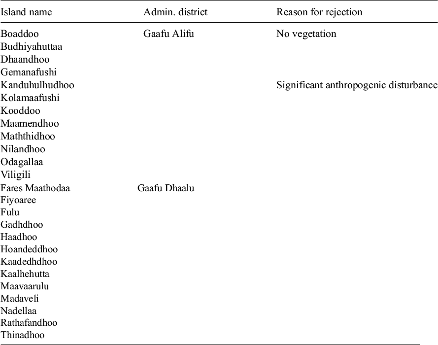

 Open access


Comments
Dear Dr. Claire Monteleoni,
We are pleased to submit our original research article, titled Disentangling Drivers of Coastal Change from Satellite Imagery to Reveal Atoll-scale Sub-annual Responses to the Indian Monsoon in the Maldives, by Myriam Prasow-Émond, Philippa J. Mason, Matthew D. Piggott, and Yves Plancherel, for your consideration for publication in Environmental Data Science.
In this study, we show how open-source, medium-resolution satellite remote sensing can be used to disentangle overlapping temporal signals - sub-annual, inter-annual and breakpoints (abrupt changes) - in a single, systematic data science framework tailored to coral reef islands. Using image segmentation and time series analysis, we analyse coastal geomorphic change across 162 islands in Huvadhoo Atoll (Maldives), where frequent monitoring remains scarce and climate-forced coastal responses are not well characterised. Our approach identifies key drivers that may compound sea level rise impacts, including the Indian Monsoon and Indian Ocean Dipole. By applying this methodology at both island and atoll scales, we uncover spatial dependencies and emerging local and regional patterns of coastal change linked to met-ocean conditions. We believe this represents a step change in how the dynamics of coral reef islands are studied in the context of climate change and anthropogenic pressures.
We believe that this paper would be a good fit for Environmental Data Science, as it presents a robust data science methodology for satellite-based time series analysis and geomorphic change detection across multiple spatiotemporal scales. While the case study focuses on the Maldives, the approach can be readily applied to other coral reef islands in Small Island Developing States.
The paper has a word count of 10,184 and contains 17 figures in the main text. The Appendix contains 1 table and 1 figure.
The authors declare that this manuscript is original, has not been published elsewhere, and does not include copyrighted material. The study was funded by the PhD President’s Scholarship at Imperial College London. As the first and corresponding author, I confirm that no generative AI was used in the scientific writing of this work. All authors have approved the final version of the manuscript. Satellite imagery data used in the paper were sourced from Copernicus, PlanetScope, NASA, and the U.S. Geological Survey archives.