1. INTRODUCTION
Increasing stability and reliability of navigation for mobile objects of different classes is becoming increasingly important. Widespread satellite navigation systems, such as the existing Global Positioning System (GPS) and Global Navigation Satellite System (GLONASS), and newly developed systems, such as Galileo, BeiDou, and others, have a fundamental defect: a vulnerability to hacking and spoofing. Satellite navigation signal transmitters have very limited power and their orbits are high (about 20,000 km). These two parameters determine the very low intensity of the received signal and create a very favourable environment for electronic attack on navigation receivers. A cheap and simple jammer can block navigation receivers at a range of some hundreds of kilometres. Moreover, contemporary advanced spoofing jammers are capable of manipulating the output information of a navigation receiver. This makes it possible to change the trajectory of unmanned aerial vehicles.
One of the possible approaches to increasing navigation systems’ robustness to countermeasures is the use of visual information of the surrounding world. In the last few years, sufficiently compact, light, and low power consumption processors have appeared. Such processors are applicable for image processing in real time for navigation on board mobile objects. Historically, the first mass use of such systems was star trackers, which were used for measuring the angular orientation of spacecraft to very high precision. Some aerial vehicles can be equipped with star trackers, for instance, the star tracker of the Optical Physics Company (OPC) (OPC, 2014). Currently, some optical navigation systems use the following objects for navigation: stars, Sun, Moon, and planets of the solar system; horizon line shape; shorelines; infrastructure objects (such as roads, dams, bridges, buildings) and Three-Dimensional (3D) reconstruction of observed surfaces and elevation maps.
For celestial navigation, and navigation by means of observation of the Sun, Moon, or planets of the solar system, it is necessary to know the local vertical orientation, which can be estimated from horizon line observation. The local vertical orientation must be accurate because an error in local vertical estimation of one angular minute causes a coordinate error of approximately one nautical mile.
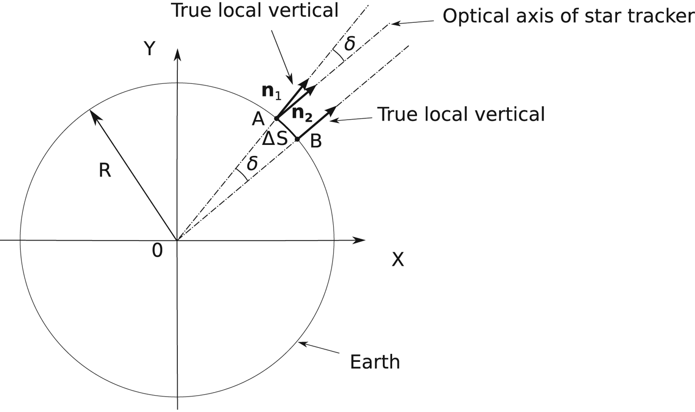
The dependence of celestial navigation error on the error of local vertical estimation is not complicated (Figure 1). Let the star tracker be at point A. The optical axis of the star tracker is directed in the direction of the local vertical. Assume the local vertical
 ${\bf n}_2$
is measured with some unknown error δ relative to the true local vertical
 ${\bf n}_1$
. There is another point B, where the local vertical has exactly the same direction as
 ${\bf n}_2$
. The navigation system will calculate the current coordinates as coordinates of point B. The error in the coordinates will be
 $\Delta S\cong R \delta$
. So, one minute of arc error produces one nautical mile error. Historically, the nautical mile was defined as one minute of latitude.
The influence of the local vertical orientation estimation error on the determination of the current coordinates.

It should be mentioned that present-day star trackers have an error of orientation estimation of about 1–6 arc sec (Blarre et al., Reference Blarre, Ouaknine, Oddos-Marcel and Martinez2006), so the error of the local vertical estimation is the main source of celestial navigation errors.
Horizon line observation is traditionally used for local vertical estimation. The use of digital elevation maps allows not only an increased precision of local vertical estimation, but also the realisation of horizon line shape navigation without the observation of stars (correlation-extremal navigation) (Dumble and Gibbens, Reference Dumble and Gibbens2015).
For the case of correlation-extremal navigation, analysis of the influence of the horizon line instability on navigation errors is much more complicated and is not detailed in this article. Atmosphere heterogeneity produces not only vertical refraction but also lateral refraction. Both of these components influence the precision of correlation-extremal navigation. Moreover, error estimation can be performed only numerically. Such estimation entails large computational costs. Estimation can be performed only for a specific area, and specific coordinates and altitude of flight. Even worse, such an estimation can be performed only for specific (real) 3D fields of atmospheric temperature and pressure. Let us consider the following example, where the altitude of flight is 370 m. From this altitude, the total range to the horizon is about 72 km. For calculation, this area is covered by a coarse mesh with a coordinate step of 10 m. So, about 2×10⁹ measurements of the atmosphere temperature and pressure (or directly of the refraction index) are required. This is a large measurement, and it is necessary to create special and very expensive devices capable of producing such measurements. Moreover, these data are constantly changing. If we use a simplified model of the atmospheric temperature and pressure, we will obtain results that do not reflect reality. Thus, incorrect initial information used for calculation will produce incorrect estimation of the navigational errors.
Let us consider what devices are used for horizon line observation. The classic example is Earth sensors of space vehicles (STD 15, 2004; STD 16, 2001; IRES, 2015). The majority of such sensors operate in the infrared band and use mechanical scanning. The error of vertical estimation ranges from about 1 to 10 angular minutes. More advanced sensors used matrix detectors (Meller et al., Reference Meller, Sripruetkiat and Makovec2000; Scheidegger et al., Reference Scheidegger, Krpoun, Shea, Niclass and Charbon2007).
Horizon line sensors are used for Unmanned Aerial Vehicles (UAVs). However, in this case such sensors are mainly used not for navigation, but for angular stabilisation (Taylor et al., Reference Taylor, Bil, Watkins and Egan2003; Ettinger et al., Reference Ettinger, Nechyba, Ifju and Waszak2002; Shabayek et al., Reference Shabayek, Demonceaux, Morel and Fofi2012; Cornall and Egan, Reference Cornall and Egan2004; Horiuchi, Reference Horiuchi2009). The precision of such sensors is poor, so they cannot be used for navigation.
Horizon line sensors are applicable for the angular orientation of mobile robots and the correction of angular errors of inertial navigation systems (Gupta and Brennan, Reference Gupta and Brennan2007; Reference Gupta and Brennan2008) and correlation-extremal navigation (Thompson et al., Reference Thompson, Henderson, Colvin, Dick and Valiquette1993; Rushant and Spacek, Reference Rushant and Spacek1998; Talluri and Aggarwal, Reference Talluri and Aggarwal1993). The local vertical estimation precision of such sensors is not very high, being
 $0{\cdot}2\hbox{-}0{\cdot}5^{\circ}$
(Gupta and Brennan, Reference Gupta and Brennan2008). The planets or other solar system bodies that have a weak atmosphere are well-suited for horizon-based navigation (Cozman et al., Reference Cozman, Krotkov, Guestrin, qtOutdoor, Position and for2000; Oiri et al., Reference Oiri, Nagatani and Yoshida2010; Nefian et al., Reference Nefian, Bouyssounouse, Edwards, Dille, Kim, Hand, Rhizor, Deans, Bebis and Fong2014; Bouyssounouse et al., Reference Bouyssounouse, Nefian, Thomas, Edwards, Deans and Fong2016; Cozman and Krotkov, Reference Cozman and Krotkov1996).
The task of optical navigation of UAVs based on horizon line images is one of the most difficult technical vision tasks. The reason is that optical measurement must be made with geodetic accuracy with very long optical traces. Effects such as scattering and absorption of light and instability of refraction in an inhomogeneous atmosphere with random parameters results in serious limitations of measurement accuracy.
Information about the local vertical orientation can be obtained not only from horizon line observation but also from observation of stars’ light refraction near the horizon (Gounley et al., Reference Gounley, White and Gai1984; Xinlong and Shan, Reference Xinlong and Shan2009; Qian et al., Reference Qian, Sun, Cai and Peng2013). This approach seems very debatable because the length of optical traces in the atmosphere is much greater in this case in comparison with optical traces in the atmosphere in the case of horizon observation. Thus, the errors caused by refraction will be much greater.
The precision of the local vertical estimation is very important because it has an impact on the precision of UAV navigation. In addition, the question of measurement precision is very important.
The first aim of this article is the experimental long-term estimation of horizon line stability. The horizon line was observed from an altitude of 370 m, which is typical for UAV flight. We used a fixed camera for continuous shooting of the horizon line, then the obtained images were processed for localisation of the horizon line with subpixel precision.
The second aim of this article is to draw attention to the significant research area of image forming at long-range and very long-range distances. It seems that the processes of image forming at such distances have not been studied sufficiently. The inaccuracy of the models and the incompleteness and inaccuracy of the initial information, results in calculations that are sometimes very far from reality. Thus, experimental studies are needed.
2. WHAT IS THE HORIZON?
Consider the horizon as a line on an image where the vertical directional derivative of brightness reaches a maximum value. Coarse estimations of vertical direction are generally known, for instance, from inertial navigation systems. This vertical direction can be used for the initial horizon line location. Then, both the vertical direction and the horizon line can be refined iteratively. There are two possible methods to form the observed horizon line. If we observe the horizon line from comparatively low altitudes, we can see the real border between the sea surface and sky. This line has been used for sea navigation for a long time. If we increase the height of the observation point, the distance to the horizon will increase as well. Accordingly, the absorption and scattering of the light in the atmosphere will increase too. From some altitudes, observation of the real horizon line will be impossible. Nevertheless, we can observe the horizon line from great altitudes. However, in this case, instead of the real horizon, we will observe some other line that will be considered as a horizon line (“false horizon”). This line will mark only the line where the vertical directional derivative of observed brightness achieves its extremum. This line is formed by the complicated processes of light propagation, absorption, and scattering in the atmosphere. The sunlight and light reflected by the Earth or sea surface take part in this process. In this case, the direction to the real horizon, which we could observe in the atmosphere without absorption and scattering, is different from the observed horizon in the real atmosphere with absorption and scattering. This is a serious distinction between unmanned aerial vehicle celestial navigation and traditional sea navigation.
The band near
 $2{\cdot}2\,{\rm \mu} \hbox{m}$
in the daytime, and bands near 3·6 and
 $4{\cdot}8\,{\rm \mu} \hbox{m}$
around the clock, are the most suitable for long-distance observation of the real horizon line (Maslov and Grishin, Reference Maslov and Grishin2013). Increases in wavelength reduce aerosol absorption and scattering effects. However, the thermal emission of the atmosphere masks the horizon line at wavelengths greater than 5 μ m. This result was obtained by calculation, but requires experimental verification. The fact is that the precision of data sources, such as atmospheric parameters, aerosol concentration, and their scattering indicatrices, cannot, for obvious reasons, have high accuracy. The atmosphere is a very unstable object with continuously changing parameters.
Nevertheless, image gathering in the visible and near-infrared bands has gained some interest. This is because cameras for this purpose are much cheaper and more accessible. However, the surface meteorological range of visibility for such cameras will be significantly less than that for infrared cameras. If we take the standard meteorological visibility range to be 23 km, the maximum altitude from which it is possible to observe the real horizon line will be about 41 m. Below this altitude, the instability of the horizon line position will be conditioned by the instability of atmospheric refraction. Above this altitude, the instability of the horizon line will be conditioned to a greater extent by the process of light propagation, scattering, and dissipation in the atmosphere.
In 2013, twenty-four hour shooting was undertaken in Simeiz (
 $44^{\circ} 24^{\prime} 44{\cdot}0^{\prime\prime} \hbox{N}$
,
 $33^{\circ} 59^{\prime} 28{\cdot}6^{\prime \prime} \hbox{E}$
) from the shore. The altitude of the shooting point was 370 m above sea level. From this altitude, the total range to the horizon is about 72 km. A Charge-Coupled Device (CCD) camera (Meade DSI Pro SONY ExView HAD™ Monochrome CCD
 $510 \times 492$
) and Mir-20 lens (F20 mm, 1:3·5) were used for shooting. Narrow-band filters of 770, 867, and 938 nm were used. A wide-band filter with a short length border of 550 nm was also used. The camera's field of view was about 12°. During shooting, the camera was motionlessly mounted. One important feature of this camera is the 16-bit analogue-to-digital converter. This is essential for measurement of the areas of extremely low contrast. Having a small number of quantification levels creates false contours, which make it extremely difficult to process the shooting results correctly. These results are used for estimating the atmospheric transparency and refraction and the stability of the horizon line (Maslov and Grishin, Reference Maslov and Grishin2015).
3. PROCEDURE FOR MEASUREMENT OF HORIZON LINE POSITION
The results of shooting with a narrow band filter of 867 nm are presented. Shooting was carried out on 8, 9, and 10 May 2013. The optical axis of the camera was directed to the south. The purpose of using this orientation is that during daytime motion the Sun should be outside the camera's field of view and thus should not hit the lens. The camera forms frames with 648 horizontal lines and 488 vertical columns. During processing, every frame is divided into eight vertical strips. The width of every strip is 61 pixels. The brightness of all 61 columns was summed in the horizontal direction and formed eight single-dimensional arrays.
Summation is significant for increasing the signal-to-noise ratio, which is low for the long distance of horizon line observation. The operation of the maximum derivative search is equivalent to searching for a zero value of the second derivative. As is known, the second derivative calculation significantly decreases the signal-to-noise ratio. The CCD matrix is characterised by a whole complex of noises.
After summation, the first coarse search for the derivative maximum in all arrays is performed. A finite impulse response filter is used for differentiation. The index with maximum response is used for coarse estimation of the horizon line position. Then, for each index in the small neighbourhood of coarse estimation, the next summation is performed in a direction that is parallel to the horizon line. For each point, the surrounding brightness of the 13 nearest points is approximated by a polynomial of the third degree:
 $$f = a\,x^3 + b\,x^2 + c\,x + d$$
To find the polynomial coefficients, the least squares method is used. The second coarse estimation of the horizon line position is determined by the maximum of the coefficient “c” of the polynomial (in other words, by the maximum of the derivative). Then for this point, we will calculate the horizon line position to subpixel precision using the formula:
 $$x = {-b}/3a$$
Such a complicated procedure is used because of the significant instability of the image statistic, which creates serious problems with subpixel resolution of the horizon line position.
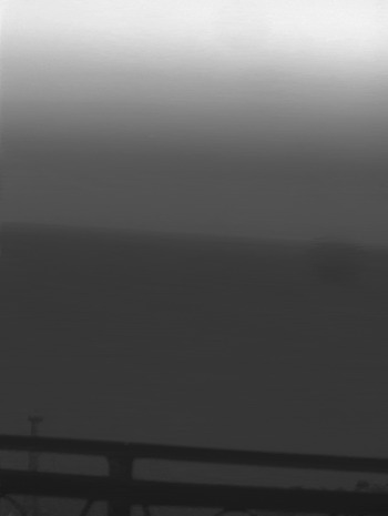
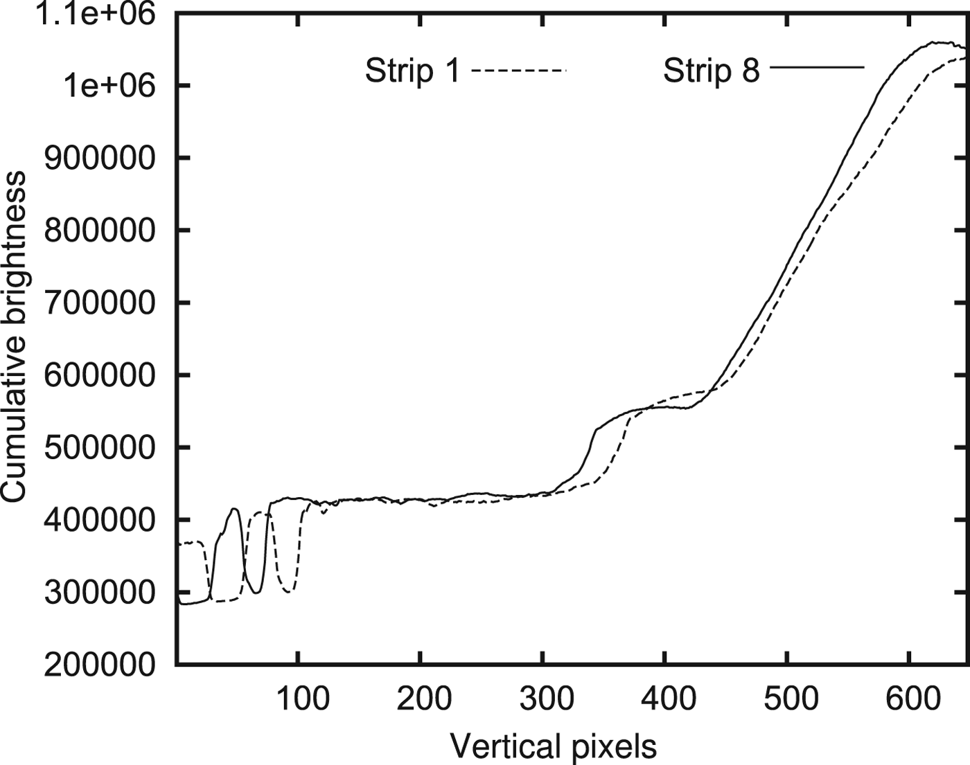
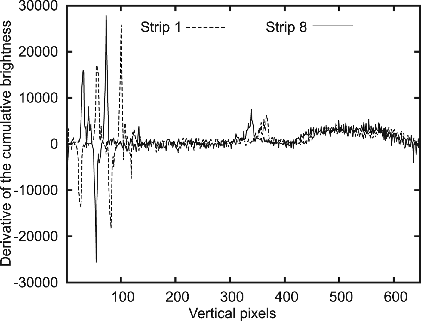
One of the shooting cadres is presented in Figure 2. The brightnesses of two strips from this cadre and their derivatives are presented in Figures 3 and 4. Two local maxima in a segment from 300 to 400 pixels mark the horizon position in Figure 4. Despite the summation, the graph shows high noise when using a simple two-point differentiation formula. This is the reason for using a finite impulse response filter for differentiation.
One of the cadres shot on 8 May 2013.

Cumulative brightness of two vertical strips in Figure 2.

Derivative of brightness of two strips in Figure 2.

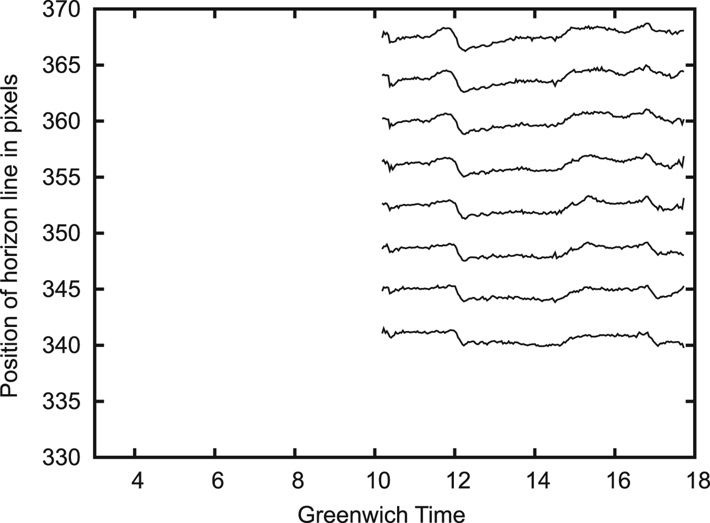
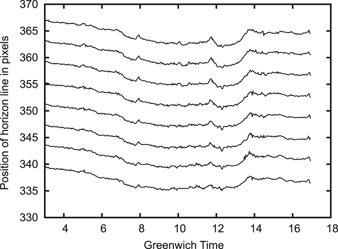
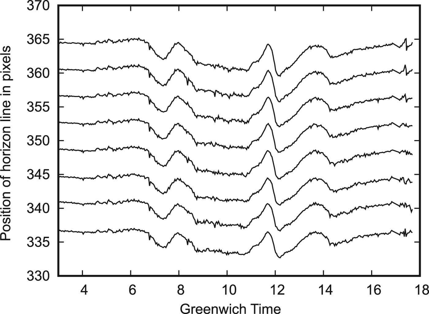
The results of horizon line position measurement are presented in Figures 5–7. The horizontal axis of these graphs shows Greenwich Mean Time (GMT). The vertical axis of the graph shows the horizon line position in pixels for each of the eight strips. The shift of the curves for different strips is conditioned by the small turn of the camera relative to the optical axis of the lens. We can see both the agreed change of horizontal position in different strips and the small variation of local inhomogeneity of the atmosphere between different strips.
Graph of horizon line position on 8 May 2013.

Graph of horizon line position on 9 May 2013.

Graph of horizon line position on 10 May 2013.

The graphs show that the interval of horizon line drift is near to 5–6 pixels (i.e. 5–7 angular minutes) during the daytime. We can see both a comparably large inhomogeneity of the atmosphere and small local fluctuations of atmospheric parameters.
It is desirable to observe the whole horizon line for estimation of local vertical orientation. Such an observation decreases the influence of small atmospheric inhomogeneities in the estimation of local vertical orientation, because the changes of atmospheric characteristics of different opposite azimuths are weakly correlated with each other. Large-sized inhomogeneities change horizon direction to the same degree for all azimuths, so the orientation of the local vertical will change very slightly. It is possible to estimate the local vertical errors in such conditions as 1–3 angular minutes. Large errors take place only when the observation point is placed on the border between two weather fronts with different temperatures. The probability of such an event is low.
4. CALCULATION OF VARIATIONS OF HORIZON LINE DIRECTION
For local vertical evaluation, it does not matter whether the observed horizon line forms as a real border between the Earth's (sea) surface and sky or only as a result of light scattering and absorption in the atmosphere (“false horizon”). This is the most significant parameter: an error of local vertical estimation. However, if we consider correlation-extremal navigation using the horizon line shape, this question will be crucial. This is because, in this case, it is not necessary to observe stars in the sky. The horizon line shape has sufficient information for navigation (Dumble and Gibbens, Reference Dumble and Gibbens2015).
Estimation of light scattering and the absorption effect on the horizon line position was calculated for 9 May 2013. The horizon image is formed as a result of the complicated process of light propagation, absorption, and scattering in the atmosphere. The program MODTRAN (MODerate resolution atmospheric TRANsmission) was used for calculation of these processes (MODTRAN, 2016). This program requires many parameters to be set before performing the calculations. One of the most important parameters that can be set is the meteorological visibility range. In Rozenbush and Vid'machenko (Reference Rozenbush and Vid'machenko2011), it was shown that the atmosphere in Simeiz has a high transparency. The closest appropriate band to the filter used with a maximum of transparency of 867 nm is the photometric band α
i
(797±149 nm). For this band, the extinction coefficient is equal to
 $\Delta m=0{\cdot}13$
. This coefficient shows a decrease of star magnitude in the atmosphere at zenith.
In astronomy, the relative brightness of stars, including the attenuation of star radiation in the atmosphere (extinction coefficient) is usually measured in logarithmic units - stellar magnitudes. There is a simple formula for recalculating the extinction coefficient in the transmittance of the atmosphere at zenith:
 $$k=10^{\lpar -0{\cdot}4\Delta m \rpar }$$
In our case, k=0·89. By means of a number of iterations of the MODTRAN calculation, the meteorological range of visibility for k=0·89 is estimated as 36 km. For the 867 nm filter, the effective band width was taken as 859–876 nm.
Calculations were performed for 36 directions of zenith angle with a step of
 $0{\cdot}03^{\circ}$
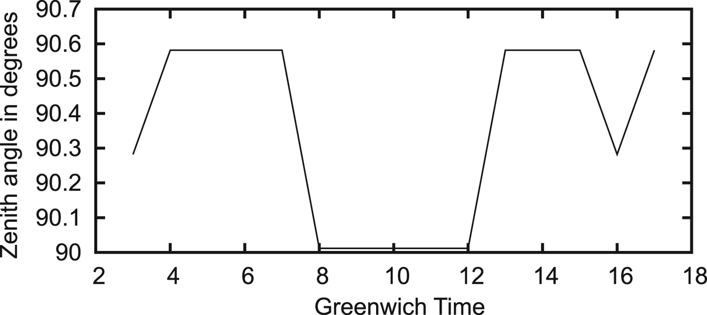
. Any smaller step is unacceptable due to errors in the contrast calculation. Brightness is calculated for the time interval from 3 to 17 h GMT. We calculated the interval of zenith angles that have maximum contrast. The middle of this interval is considered as the horizon line direction. The results of the calculation are shown in Figure 8. The anomalous value at 16 h GMT seems to be due to the errors in contrast calculation in the area of very low contrast.
Calculated horizon line zenith angle for 9 May 2013.

It is interesting that in the morning and evening hours, the zenith angle of the horizon equals
 $90{\cdot}582^{\circ}$
. This value differs from that found by considering only refraction for the MODTRAN model of the atmosphere (that is
 $90{\cdot}574^{\circ}$
) by only
 $0{\cdot}008^{\circ}$
. If we take into account that the step of the zenith angle calculation was equal to
 $0{\cdot}03^{\circ}$
, we can conclude that according to the calculation, we observe the real horizon during some morning and evening hours. Near to local noon, solar lighting achieves its maximum, and the derivative of solar radiation scattered by the atmosphere exceeds the contrast between the sea surface and sky. Therefore, the horizon line will be observed at the zenith angle of
 $90{\cdot}012^{\circ}$
. The total interval of the horizon zenith angle is
 $0{\cdot}57^{\circ}$
or 34·2 angular minutes. In other words, there are two competing mechanisms of horizon line formation. However, the experimental interval of horizon line direction drift is much less than 34·2 angular minutes. Thus, we can conclude that the experimental results show only one mechanism of horizon line formation.
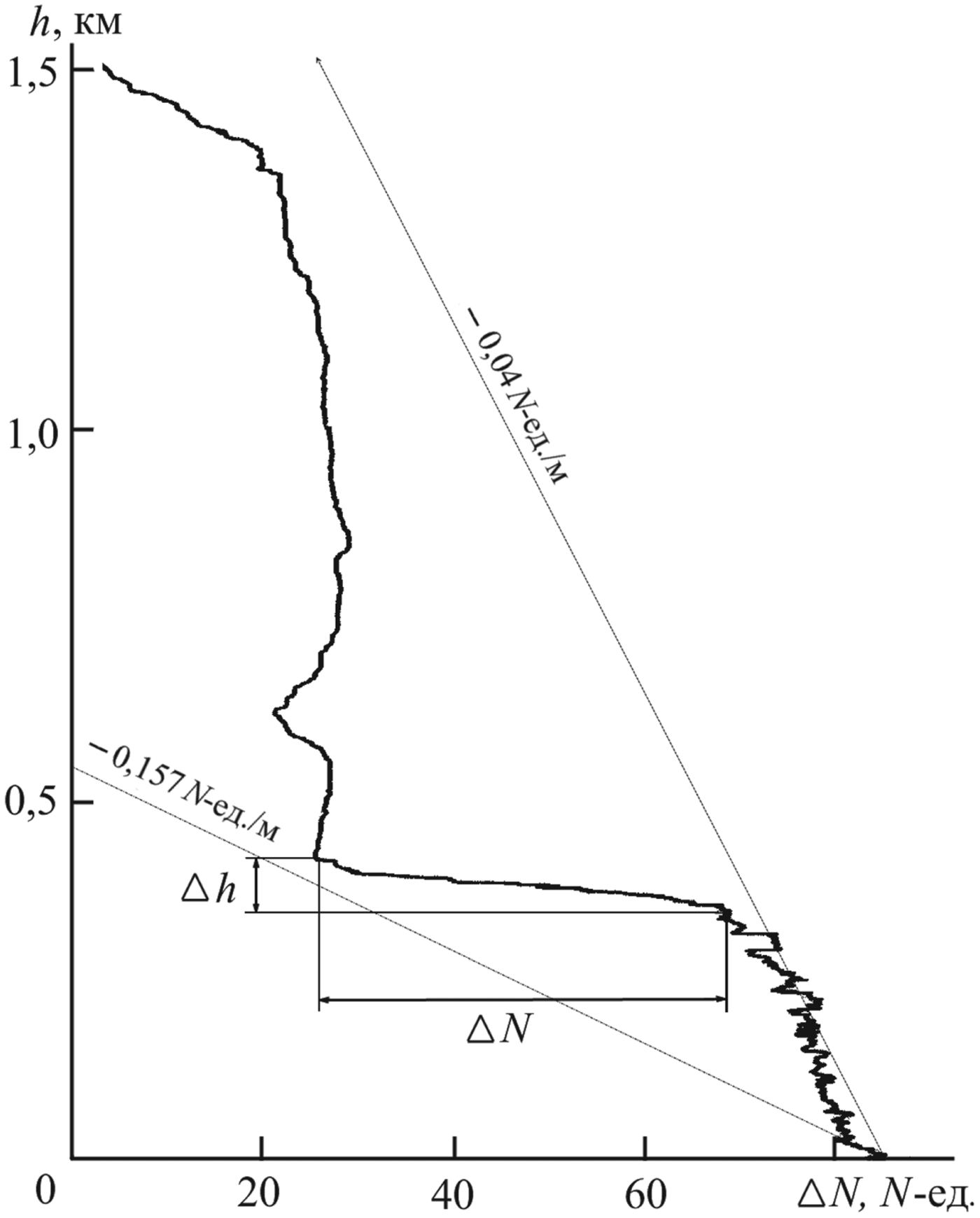
Another factor that affects the shift of the visible horizon line is refraction instability in the layered atmosphere. The results of experimental research on the refraction index over the Black Sea are presented in Kabanov (Reference Kabanov2009). In particular, the real altitude profile of the refraction index is shown in Figure 9 and is presented in N units:
Measured profile of refraction index over the Black Sea (Kabanov, Reference Kabanov2009).

 $$n = \lpar n-1 \rpar \times 10^6,$$
where n is the refraction coefficient.
The horizontal axis of the graph shows the increment of the refraction index in N units relative to a basic level. The vertical axis of the graph shows altitude. The significant unevenness in the refraction index is governed by stable layers in the atmosphere that have a temperature inversion. Usually atmospheric temperature decreases with increasing altitude but in some altitude intervals, temperature can increase. This effect is called temperature inversion and is widespread (Iacobellis et al., Reference Iacobellis, Norris, Kanamitsu, Tyree and Cayan2009). Figure 9 shows temperature inversion in the segment of altitudes approximately from 350 to 420 m. Such layers, despite their stability, are capable of quickly changing altitude (up to 50–100 m in 10 min). In summer, such layers can be positioned at a height from tens of metres up to 600 m. These layers can be formed by sea breezes, mountain valley winds, and other factors.
Unfortunately, the refraction index in Kabanov (Reference Kabanov2009) refers to the radio frequency band. For calculation of the refraction index for the optical band, it is necessary to know the vertical profile of water vapour partial pressure and the temperature profile. The refraction index for the radio frequency band (ITU, 2003) is:
 $$N = {77{\cdot}6 \over T}\left(P + {4810e \over T} \right) = {77{\cdot}6P \over T} + {77{\cdot}6 \times 4810e \over T^2},$$
where P is atmosphere pressure, T is absolute atmospheric temperature, and e is the partial pressure of water vapour. For the optical band, the second summand in Equation (5) disappears.
We can compare the effect of the atmospheric temperature and pressure on the refraction index. The derivatives are:
 $$\eqalign{dN/dT & = -77{\cdot}6P / {T^2}\cr dN / dP &=77{\cdot}6 / T}$$
For
 $P_{0} = 1013{\cdot}25\,\hbox{hPa}$
and the temperature at sea level T=293 K, these derivatives are:
 ${dN} / {dT} = -0{\cdot}916$
and
 $dN / dP = 0{\cdot}265$
. We can conclude that temperature variation has a greater effect on the refractive index than pressure variations. Moreover, significant temperature variations are much more probable then pressure variations. If we do not consider such extreme atmosphere phenomena as tornados, the spatial horizontal pressure gradients are small because such gradients generate a wind equalising the pressure. At the same time, with a weak wind, significant temperature gradients are very likely because of the low rate of heat exchange in a calm atmosphere. Atmospheric mirages are generated by just such temperature gradients.
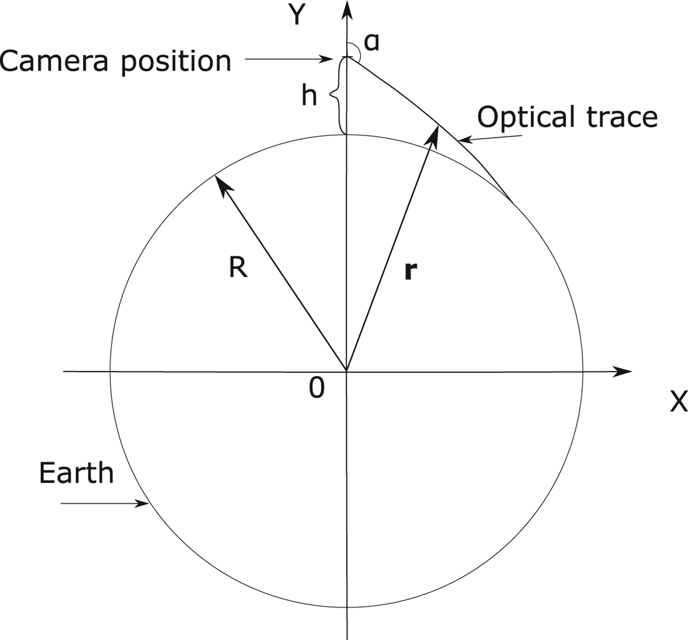
Let us calculate the influence of temperature inversion intensity on the light refraction in the atmosphere. Suppose that temperature inversion is located below the altitude of the shooting camera, for instance from 250 to 320 m. Figure 10 shows the geometry of this task.
Geometry of the task.

On this chart, h is the altitude of the camera position (h=370 m), α is the zenith angle of the optical trace
 $(\alpha \gt 90^{\circ})$
and R is the radius of the Earth (6,371·2 km). A program for calculation of light propagation considering refraction was developed on the basis of the eikonal equation (Kravtsov and Orlov, Reference Kravtsov and Orlov1990).
 $$\eqalign{{d\,{\bf r} \over d\tau} &= {\bf p} \cr {d\,{\bf p} \over d\tau} & = {1 \over 2} \nabla n^2\lpar {\bf r} \rpar ,}$$
where
 ${\bf r}$
is the radius vector and n is the refraction coefficient:
 $$n = 1 + 10^{-6}\ N = 1 + 10^{-6} {77{\cdot}7P \over T},$$
where P is atmospheric pressure and T is the absolute atmospheric temperature.
The initial conditions for this equation are:
 $$\eqalign{{\bf r} & = \lpar 0,\quad R + h \rpar \cr {\bf p} &= \lpar \sin \lpar \alpha \rpar , \quad \cos \lpar \alpha \rpar \rpar }$$
Atmospheric pressure is calculated from the formula:
 $$P = P_0 \exp \left(-{g \over R_b} \int\limits_0^h {dh \over T} \right),$$
where P 0 is atmospheric pressure at sea level, h is altitude above sea level, g is gravitational acceleration, T is the absolute temperature of the atmosphere (K), and R b is the specific gas constant:
 $$R_b = {R \over M},$$
where R is the universal gas constant and M is the molar mass of Earth's air.
The differential equation was solved by the Runge-Kutta method for atmospheric pressure
 $P_{0}= 1013{\cdot}25\,\hbox{hPa}$
(ITU, 1997) and temperature at sea level T=293 K. The vertical gradient of the atmospheric temperature outside temperature inversion is set equal to
 $0{\cdot}055^{\circ}/\hbox{m}$
for summer time. The horizon line direction is calculated by a sequential ray-tracing calculation for different zenith angles with a step of
 $0{\cdot}001^{\circ}$
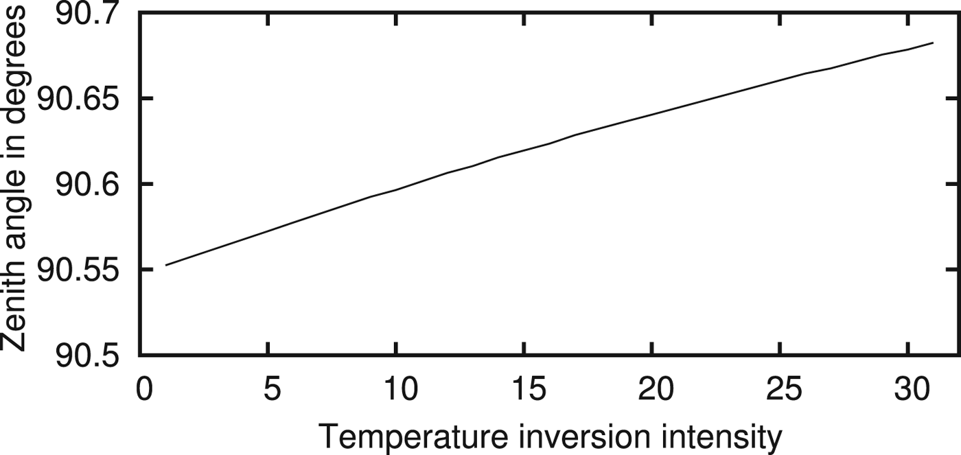
. The results of this calculation are presented in Figure 11. The horizontal axis corresponds to the temperature inversion intensity, while the vertical axis corresponds to the horizon line zenith angle. The temperature inversion intensity changed over an interval of 1–31°C.
Horizon zenith angle as a function of temperature inversion intensity.

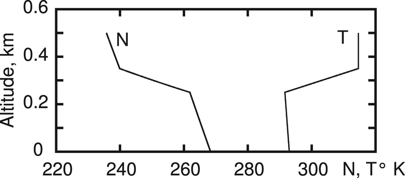
The inversion intensity of 23° led to a change in the zenith angle of horizon observation of 7 angular minutes. The vertical profile of temperature and refraction index in N units for the temperature inversion intensity of 23° is presented in Figure 12.
Vertical profile of temperature and refraction coefficients.

It should be mentioned that this calculation is approximate because a spherically symmetrical model of the atmosphere is used for calculation. More precise calculation requires much more information (3D fields of atmospheric pressure and temperature).
Unfortunately, we could not find statistics on the inversion over the Black Sea, so we used data from Iacobellis et al. (Reference Iacobellis, Norris, Kanamitsu, Tyree and Cayan2009). It follows from this report that such intensity inversions are not unique. Most of the inversions in California have an intensity of more than 10°. We cannot, however, exclude the influence of the change of aerosol concentration in the air on the value of the measured horizon line bias. The calculations of this effect are much more difficult and much less reliable then refraction calculation. It is for these reasons that experimental studies are much more preferable for long-range visual navigation.
5. DISCUSSION
Generally speaking, the variation of refraction can be much greater than the values that we have obtained. High-precision estimations of atmospheric refraction were carried out in Schaefer and Liller (Reference Schaefer and Liller1990), Young (Reference Young2004) and Sampson et al. (Reference Sampson, Lozowski, Peterson and Hube2003). In these works, the times of sunset and sunrise were measured. The variation of these times represents variations of atmospheric refraction. The measurements show that the range of refraction scatter is near
 $0{\cdot}234\hbox{-}1{\cdot}678^{\circ}$
(Schaefer and Liller, Reference Schaefer and Liller1990) and
 $0{\cdot}402^{\circ}\hbox{-}2{\cdot}081^{\circ}$
(Sampson et al., Reference Sampson, Lozowski, Peterson and Hube2003). At the same time, the horizon line position varies in the range from
 $-0{\cdot}246^{\circ}$
to
 $0{\cdot}326^{\circ}$
(Young, Reference Young2004).
Grelsson et al. (Reference Grelsson, Felsberg and Isaksson2015) presents the results of the estimation of errors in local vertical measurement by means of horizon line observation:
 $0{\cdot}02^{\circ}$
or 1·2 angular minutes (mean error). Apparently, such high precision of local vertical estimation is possible in a sufficiently homogeneous and stable atmosphere during a short period of observation.
Another problem exists in the area of horizon observation. The problem is what we see: Is there a real horizon or it is a “false horizon”, conditioned by light scattering and absorption in the atmosphere? Generally speaking, the question of the possible maximum observation distance of objects is complicated. For instance, the La Encantada Mountain on peninsular California is visible from the Californian Gulf in the presence of strong refraction at a distance of about 200 km (Ronald, Reference Ronald1968). However, this distance is several times greater than the meteorological range of visibility for the best conditions of observation. Experiments (Janeiro et al., Reference Janeiro, Wagner, Ramos and Silva2007a; Reference Janeiro, Wagner, Ramos and Silva2007b) show that under favourable viewing conditions in Europe, the visibility range can reach values of the order of 100 km. On the other hand, in Shipunov and Semashkin (Reference Shipunov and Semashkin2011), it is shown that the meteorological visibility range has serious dispersion and is of the order of only tens of kilometres. The probability of a large meteorological visibility range is small. Obtaining a more accurate answer regarding the observability of the real horizon line is possible only by implementation of experimental studies with specially developed instruments similar to those in Shields et al. (Reference Shields, Johnson and Karr1992) and Shields et al. (Reference Shields, Karr, Johnson and Burden2013). Improved versions of such instruments are currently used. Unfortunately, significant funds are required for the development of such instruments. Instruments should be operated in different bands of visual and infrared light. Such instruments should be used for round-the-clock monitoring of the horizon line. For the accumulation of statistics, instruments should operate over years in different regions of the ocean and at different altitudes. The possibilities for the development of such instruments in Russia are very limited. The joint project “Development of a Computer Vision Navigation System” (CORDIS, 2017) was designed to develop such instruments.
This leads to the practical application of celestial navigation. It seems that the low accuracy of local vertical estimation is a significant obstacle to the use of stellar navigation. Nevertheless, optical navigation and inertial navigation are the last navigation resorts in conditions when all other radio navigation systems are out of operation. Global Navigation Satellite Systems (GNSS) are well known, but are also a vulnerable navigation system. In addition, other radio navigation systems can also be jammed. There are no serious technical problems for this, and jamming methods were developed many years ago. Optical navigation systems are passive systems and for this reason are very difficult to interfere with. To improve the accuracy of measurements, it is desirable to develop a sensor which can observe the whole horizon line (for all azimuths). When the shore appears in sight of an optical navigation system, correlation-extremal navigation on the shape of the horizon line becomes possible. This can reduce the navigation error to dozens, or in the worst case, hundreds of metres. Observation of shore landmarks will further decrease the navigation errors to the order of tens of metres or less.
6. CONCLUSIONS
Measurements show that during the day, zenith angle variations of the horizon line were close to 5–7 angular minutes. Calculation of light propagation, absorption, and dissipation shows that there are two possible mechanisms of horizon line formation. The first assumes observation of the real horizon line as a border between the sea and sky. Another mechanism assumes observation of the line that consists of the points of the maximum vertical directional derivative of brightness of light scattered by the atmosphere (“false horizon”). However, in reality, only one of these mechanisms exists. A very rough estimate of the variation of refraction in the atmosphere does not rule out that there could be a real horizon.
In this article, it is shown that atmospheric refraction in temperature inversions has a serious impact on the observed horizon direction and hence on the precision of local vertical estimation. The greater the altitude of flight, the lower the accuracy of local vertical estimation. We can also note that in the case of correlation-extremal navigation, horizontal gradients of atmospheric pressure and temperature are more important.
We conclude that, first, it should be taken into consideration that, as the altitude of UAV flight increases, the accuracy of the local vertical direction estimation decreases as compared with marine ships, due to the influence of refraction. An additional factor that reduces the accuracy of measurements is the appearance of a “false horizon” at a certain altitude. Secondly, it is desirable to use all azimuth horizon line sensors to increase the accuracy of local vertical estimation. Finally, we recommend that to improve the accuracy of optical navigation, the processes of image forming at long-range and very long-range distances should be studied more carefully. The existing approximate models of image forming sometimes demonstrate results that are far from reality.
The most important topic for future research is the development of a device which is capable of shooting in three spectral bands and in polarised light. The aim is to determine the most appropriate methods for horizon observation. In addition there is a requirement to measure directions on the horizon line relative to stars for clarification of the origin of the observed horizon line. Is it a real or “false” horizon?
FINANCIAL SUPPORT
This work was supported by the Russian Foundation for Basic Research under grant no. 12-08-00863-a.