







1. Introduction
This paper explores a particular type of buoyancy-driven instability that arises in the industrial process of plug cementing. Plug cementing is a relatively common operation that is carried out in both the construction and later decommissioning of an oil or gas well. In this process, a cement slurry (typically with a density of  $1600\unicode{x2013}1900\ {\rm kg}\ {\rm m}^{-3}$) is pumped down a small-diameter pipe into the well and is discharged at a certain depth. As the slurry is pumped to fill the full diameter of the well, the pipe is slowly withdrawn. This allows the length of cement to hydrate and plug the well when solid (Nelson & Guillot Reference Nelson and Guillot2006). One reason for the plug might be to serve as a stable base for redirecting the well trajectory during the drilling phase. In this case only the mechanical integrity matters. Alternatively, at end of life when decommissioning a well, a series of cement plugs are set at different depths in the well in order to provide a hydraulic seal. The hydraulic resistance is gained by ensuring a long length of cement plug and a good hydraulic bond to the interior steel casing (Opedal et al. Reference Opedal, Todorovic, Torsaeter, Vrålstad and Mushtaq2014; Trudel et al. Reference Trudel, Bizhani, Zare and Frigaard2019; Vrålstad et al. Reference Vrålstad, Saasen, Fjær, Øia, Ytrehus and Khalifeh2019; Kamali, Khalifeh & Saasen Reference Kamali, Khalifeh and Saasen2022). Thus, concerns such as mixing and contamination of the cement are relevant.
There are many interesting fluid mechanics questions concerning the plug cementing process in its many variations. It is possible that the cement slurry is pumped on top of a mechanical support placed in the well, in which case the placement is generally not problematic (Khalifeh & Saasen Reference Khalifeh and Saasen2020; Harestad et al. Reference Harestad, Karimfazli, Ghazal, Harestad and Saasen2023). However, positioning of the mechanical support (bridge plug, retainer, etc.), requires additional time and cost. Therefore, it is relatively common that the cement slurry is simply pumped on top of another fluid: a so-called off-bottom plug. The fluid supporting the slurry may be the drilling fluid in the well, or a specially mixed viscous pill, or even freshwater. The former is more likely to occur when the plug is set during construction. Freshwater is more likely at decommissioning. It is the latter that we study. The issue with all of these scenarios is that the cement slurry is invariably denser than the fluid underneath, i.e. in a mechanically unstable configuration. How then can the cement remain in place for long enough that it may hydrate?
During the late 1980s and early 1990s the practice of drilling deviated wells became more popular. For such wells a short kick-off plug was often needed to redirect the drillpipe trajectory. It was observed that, when set off-bottom, many of these plugs failed, meaning that they were not found to be present in the well at the depth expected when subsequently tagged with the drillpipe. Indeed Heathman et al. (Reference Heathman, Carpenter, Marcel, Rimer and Badalamenti1994) and Heathman (Reference Heathman1996) reported that more than 2 attempts were needed for each successful plug. In an interesting experimental study Calvert, Heathman & Griffith (Reference Calvert, Heathman and Griffith1995) reported that a common failure mode involved the heavy slurry sliding under the lighter supporting fluid in an exchange flow. Various procedures were recommended in order to stabilise the flow (Calvert et al. Reference Calvert, Heathman and Griffith1995). These studies are all practically relevant to the current topic, in that they define the initial state of the fluids in the post-placement phase.
A series of studies followed, focused on the slow viscous slump flows that were observed during failure (Frigaard Reference Frigaard1998; Frigaard & Scherzer Reference Frigaard and Scherzer1998; Crawshaw & Frigaard Reference Crawshaw and Frigaard1999; Frigaard & Crawshaw Reference Frigaard and Crawshaw1999; Frigaard & Scherzer Reference Frigaard and Scherzer2000). Cement slurries have a moderate yield stress. Thus, although a Newtonian–Newtonian pairing of heavy fluid above light fluid is unstable (the classical Rayleigh–Taylor configuration), the same is not true of a yield stress fluid. Indeed, it is possible to derive criteria for the yield stresses required to stabilise the interface between two yield stress fluids (Crawshaw & Frigaard Reference Crawshaw and Frigaard1999; Frigaard & Crawshaw Reference Frigaard and Crawshaw1999). This direction is reviewed later in § 3.1.
While the above was relevant to setting plugs used during well construction, the plug and abandonment (P&A) operation does not quite fit the same physical setting. In the decommissioning process, the well is to be sealed permanently and consequently the inside of the casing is generally washed/flushed prior to plug placement. A non-corrosive fluid is then left inside the casing, often freshwater in Western Canada, with the cement set on top. For off-bottom plugs this results in parameter ranges where the density difference is very large and the lower fluid has no yield stress and low viscosity. The dimensionless yield numbers typically found are far below the targets set in Crawshaw & Frigaard (Reference Crawshaw and Frigaard1999) and Frigaard & Crawshaw (Reference Frigaard and Crawshaw1999) to arrest fluid motion.
This has led to a renewed effort to understand how off-bottom P&A plugs might be stable. One difference with well construction plugs is that the lengths of cement slurry in P&A can be many 10s to 100s of metres, according to the surrounding geology and the regulations; see Trudel et al. (Reference Trudel, Bizhani, Zare and Frigaard2019). This means that a successful P&A plug might tolerate a limited amount of instability/mixing at the lower end, while still providing an effective seal. Thus, more research has been targeted at understanding the placement process and subsequent fluid motions.
Plug placement has been studied extensively by Ghazal & Karimfazli (Reference Ghazal and Karimfazli2021, Reference Ghazal and Karimfazli2022a,Reference Ghazal and Karimfazlib) using two-dimensional (2-D) computational simulations. Ghazal & Karimfazli (Reference Ghazal and Karimfazli2021) consider vertical injection of a Bingham fluid (cement slurry) into a Newtonian fluid within a deep closed duct (well), over a range of Reynolds, Froude and Bingham numbers. The miscibility of the fluids is varied via an artificial Péclet number, considered in 3 ranges. A variety of flows are observed, but the typical sequence involves: (i) penetration of the Bingham fluid downwards with consequent displacement of the in situ fluids upwards around the injector; (ii) onset of instabilities at the interface of the descending stream; (iii) mixing across the width of the duct coupled to upwards displacement of the injected fluid around the injector. Ghazal & Karimfazli (Reference Ghazal and Karimfazli2022b) have studied a wide range of injector sizes and positions (representing eccentricity in the well). Although there are differences in the upwards flow due to the geometry, the basic message is that the flow below the injector is stabilised by mixing across the duct. This forms a gradient of densities in a mixed region between the fluids. Later studies have considered other operational features such as removing the pipe from the plug in the balanced plug method (Ghazal & Karimfazli Reference Ghazal and Karimfazli2022a; Harestad et al. Reference Harestad, Karimfazli, Ghazal, Harestad and Saasen2023).
There have also been a number of studies that investigate the motion of fluids below an injection pipe using laboratory experiments. Varges et al. (Reference Varges, Fonseca, Costa, Naccache, de Souza Mendes and Pinho2018) placed Carbopol gels above less dense light vegetable and mineral oils in a vertical pipe, separated with a sliding gate valve. Many interesting exchange flow patterns were observed, both stable and unstable. Akbari and co-authors have systematically studied the placement of fluids into a pipe in a related P&A process called dump bailing (Akbari & Taghavi Reference Akbari and Taghavi2020, Reference Akbari and Taghavi2021, Reference Akbari and Taghavi2022a,Reference Akbari and Taghavib, Reference Akbari and Taghavi2023). In this process the fluids are dumped from a tube onto a mechanical support, from a height of many diameters above. There are similarities with plug cementing in the flows just below the tube, but in dump bailing the injection velocity is not controlled (it is a drainage flow). In these studies, effects of (well) inclination, dumping height, fluid rheology and other geometrical features are studied. Certainly, there are regimes in which the fluids mix effectively on exiting the tube, but others in which e.g. a thick column of the placed Carbopol descends in a coil-like structure into the water below (Akbari & Taghavi Reference Akbari and Taghavi2022b). In relation to the computational studies of Ghazal & Karimfazli, we also need to note that the dumping height in the experiments is generally smaller, i.e. these are not all properly off-bottom placements. Aside from these studies there is also a significant body of experimental work that has considered yield stress fluid displacement flows, in pipes of similar diameter as here and with Carbopol as one of the fluids (Gabard & Hulin Reference Gabard and Hulin2003; Alba et al. Reference Alba, Taghavi, de Bruyn and Frigaard2013; Amiri et al. Reference Amiri, Eslami, Mollaabbasi, Larachi and Taghavi2019; Kazemi et al. Reference Kazemi, Akbari, Vidal and Taghavi2024). While not usually directly relevant, due to the imposed flow rate, these studies can exhibit similar phenomena at the lower flow rates and where buoyancy becomes dominant.
For our study, we consider the phase after placement/injection. The evidence reviewed above suggests that successful placement may be achieved (Ghazal & Karimfazli Reference Ghazal and Karimfazli2021, Reference Ghazal and Karimfazli2022b). However, the placement phase is driven by pumping that provides energy to the flow, which may be important in the stabilising mixing flow that is observed. Once the pipe is removed from the well and the pumps stopped, the heavy cement slurry must still remain above the lighter fluid for a period of many hours in order to hydrate and form a solid plug. If the flow is unstable, a small amount of water penetration upwards into the cement slurry is unlikely to be critical (considering the lengths of cement), simply altering the water-to-cement ratio locally (Nelson & Guillot Reference Nelson and Guillot2006). However, we would like to understand the worst-case scenarios for such flows, which we consider likely to occur without any pre-mixed zone separating the fluids.
Consequently, we consider the stability of a heavy fluid over a light fluid separated initially via a gate valve. The upper fluid is a Carbopol solution, with a yield stress controlled via the concentration and density increased using glycerin or sugar. The lower fluid is generally water. We have reported results of our preliminary experiments in Vogl et al. (Reference Vogl, Waldal, Sarmadi, Fershtman, Mitishita and Frigaard2022) and Charabin & Frigaard (Reference Charabin and Frigaard2023). The first of these provides a phenomenological descriptions of early experiments, including below the gate valve, but did not compute front velocities or otherwise quantify the flows. Charabin & Frigaard (Reference Charabin and Frigaard2023) presented results from 8 early experiments, but with little post-processing or classification. Here, we give a more comprehensive report on the full range of experiments performed, together with comparisons with dimensional analysis and simplified models. The questions we seek to answer include: (i) first confirming the previous stability studies (Crawshaw & Frigaard Reference Crawshaw and Frigaard1999; Frigaard & Crawshaw Reference Frigaard and Crawshaw1999); (ii) classifying and understanding the different flow types when static stability is not immediately possible.
An outline of our paper is as follows. First, directly below we outline the experimental methodology used (§ 2.1), present example results (§ 2.3) and introduce the main relevant dimensionless groups (§ 2.4). The results start in § 3 by confirming the division of our flows into static or flowing configurations, then classifying the latter. Examples are given of each of the observed flow types. Section 3.3 introduces a 1-D lubrication model that helps us understand our flows at the stage when the interface elongates along the pipe. Later we try (§ 3.4) to apply a recent predictive energy theory for the finger width. The paper ends with a discussion (§ 4).
2. Methodology
Our paper primarily addresses the questions outlined in § 1, through a targeted experimental study. The basic experiment consists of positioning a dense visco-plastic fluid above a less dense Newtonian fluid (water) and observing the flow. In Vogl et al. (Reference Vogl, Waldal, Sarmadi, Fershtman, Mitishita and Frigaard2022) we have covered experimental ranges where the yield stress of the upper fluid is large enough to prevent flow. The focus of our study is therefore on smaller yield stresses, for which flow initiates due to the mechanically unstable configuration.
We are interested to quantify the speed at which failure occurs, which we quantify via the speed at which the light fluid is observed to rise through the heavier fluid:  $\hat {V}_L$. This is measured for each experiment and used to both define relevant dimensionless groups and to quantify the various flow regimes that are observed. We have performed approximately 40 unique experiments with fully characterised fluid rheologies, with some additional repeats. In addition, some of the experiments from Vogl et al. (Reference Vogl, Waldal, Sarmadi, Fershtman, Mitishita and Frigaard2022) are included where flow is prevented:
 $\hat {V}_L = 0$.
2.1. Apparatus and procedure
Our experiments were performed in an experimental apparatus with total length  $2\hat {L} = 3.05\ {\rm m}$. The flow occurs in a circular Plexiglas pipe of radius
 $\hat {r} = 9.53\ {\rm mm}$. Figure 1 shows a schematic of the experimental set-up; see also table 1. The pipe is encased in a boxed aquarium filled with glycerin with refractive index
 $n_g = 1.47$, similar to that of the Plexiglas, to offset the refractive effects. In order not to contaminate the two fluids at the start of the experiment, the pipe is split into two equal sections of length
 $\hat {L}$, separated by a pneumatically actuated gate valve that seals the two separate fluid domains. This allows the user to control when the fluids first contact. All experiments are conducted in a vertical configuration. A hydraulic leg mounted to the rigid frame allows the apparatus to rotate from
 $0^\circ$ to
 $\text {90}^\circ$. The circular pipe is backlit with an LED lighting strip with a light diffuser to reduce background noise. Two cameras are used to analyse the experiments. The first camera (Nikon Z5), images the upper half of the pipe, starting just above the gate valve, which we define to be (
 $\hat {z} = 0$), up to a length of
 $\hat {z} = 1300 \ {\rm mm}$, and is located
 ${\sim }1\ {\rm m}$ away from the apparatus. The second camera (Nikon Z50), is positioned closer to the pipe:
 ${\approx }0.3\ {\rm m}$ back from the tube and
 $\text {2}/\text {3}$ upwards from the gate valve to allow close view imaging of any instability.
Schematic of the experimental section. The viscoplastic fluid is positioned above the gate valve. The light fluid dyed and placed below the gate valve.

Main dimensional parameters for our study, along with their experimental ranges.

A strict protocol related to preparing the experiments was implemented to be consistent between each experiment. The pipes were initially flushed with water to clean any residual fluids still in the pipe from previous experiments. The light fluid was dyed black for contrast and is pumped through the pipes at the lowest flow rate possible to reduce bubble entrapment. Once the light fluid has filled the pipes, the apparatus was sealed and left to stand for 10–15 min to let bubbles rise from the solution. The gate valve is then opened and closed to allow any bubbles to detach from the gate valve. Finally, the gate valve is closed to isolate the upper part of the pipe. A valve at the bottom of the upper pipe is then used to drain the light fluid and replace it with the heavy fluid of choice. Since the heavy fluid contains a yield stress, bubbles of a small radius do not necessarily escape when static. We circulate the heavy fluid slowly until only microsize bubbles remain. The heavy fluid valve is then shut. The apparatus is filled with heavy fluid over light fluid, in two separate pipes connected through the gate valve.
To start the experiment the cameras are turned on to record at 4 K resolution with 24 fps. The pneumatic gate valve is opened, taking approximately  $1$ s. The cameras record the motion, for which the main driving force is buoyancy. Usually a finger of the light fluid is observed to initially form and propagate upwards into the heavy fluid, within a few minutes from opening. If this instability does not occur within 10 min, the system is classified as stable and the experiment halted.
To process the images obtained, the light intensity is normalised by subtracting a reference image; in our case, this reference image is the first image. This eliminates any background noise that is constant throughout the experiment, so we are only left with the light intensity in the pipe. This intensity is normalised  $I_{norm} = (I - I_{min})/(I_{max} - I_{min})$, which scales the intensity between
 $0$ representing the less dense fluid (dark colour) and
 $1$ representing the denser viscoplastic fluid (light colour). The images are post-processed to extract a representative front velocity
 $\hat {V}_L$, and to classify other features of the dynamics, as described later. Selected experiments were repeated twice to verify reproducibility. These were found to have variations in
 $\hat {V}_L$ below 5 %.
2.2. Fluid preparation
Throughout our study, the light lower fluid was tap water coloured with ink. The denser upper fluid was made by using a base of either tap water or glycerin to which Carbopol 940 polymer was added. Carbopol 940 was chosen due to exhibiting a yield stress while being relatively inelastic and also not showing significant aging effects. Weight concentrations (wt $\%$) ranged from 0.07 wt
 $\%$ to 0.15 wt
 $\%$, allowing experiments over a wide range of yield stress values. The density of the heavy fluid was varied using either sugar or glycerin: both allowed the density to vary from
 $1050$ to
 $1250\ {{\rm kg}}\ {{\rm m}}^{-3}$. At this maximum density, sugar would no longer dissolve into the water, and glycerin solution approaches its maximum value of
 $\hat {\rho }_{glycerin} \simeq 1260\ {{\rm kg}}\ {{\rm m}}^{-3}$. Note that the glycerin is always diluted with some water to prevent residual glycerin from sticking to the pipe, affecting future experiments, i.e. it eases cleaning.
To create the Carbopol–water solutions 10 l of the base fluid was put under a mixer at 270 rpm. The Carbopol was then slowly dispersed into the base fluid according to the desired wt%, paying careful attention not to allow clumps to form. The solution is then mixed for two hours. Since Carbopol is acidic ( $pH \simeq 2.7\unicode{x2013}3.3$), the solution is neutralised by adding 10 % sodium hydroxide (NaOH) and testing the pH. The solution was mixed for an additional hour, allowing complete homogenisation. For the glycerin base, the procedure was similar except water and glycerin were premixed to attain the desired density. The glycerin is much thicker than the water–sugar base, so care is needed to ensure that no Carbopol is attached to the side of the bucket or the blade. Also a longer time is needed to homogenise the mixture. The mixing proceeds for 3–8 h, with increasing time for the higher densities. The NaOH is added after approximately 2 h After either solution is made, the sample is capped and rested for 24 h. Mixing of both solutions is done by a digital EUROSTAR© 60 mixer and a three-bladed stainless steel blade, which provides constant mixing behaviour.
Although a consistent preparation protocol is followed, the key point is to have homogenous solutions of the target density, rather than any specific rheology. Samples of the upper fluid are taken for each experiment to measure the density and rheology. A Kinexus Ultra $^+$ rotational rheometer was used to characterise the heavy fluid rheological behaviour. Figure 2 shows a typical flow curve and fit to the Herschel–Bulkley model for one of the samples. Controlled strain rate tests were used with ramp-up and ramp-down cycles over a range of
 $10^{-3} \leq \dot \gamma \leq 10^{1}\ (\text {s}^{-1})$, to cover the range of strain rates typical in the experiments. A serrated parallel plate geometry was used to minimise wall slip: diameter 60 mm and gap width 1 mm. Before each cycle, the fluid was presheared at
 $15\ \text {s}^{-1}$ for 60 s, followed by a zero applied rate for 60 s. Along with the controlled strain rate test, an amplitude sweep test was also performed to characterise the linear viscoelastic regions at varying strain
 $\%$ with a fixed frequency of 1 Hz. The inset of figure 2 shows results for the same fluid. At low strain
 $\%$, the heavy fluid experiences linear elastic response: the storage modulus (
 $G^{\prime }$) and loss modulus (
 $G^{\prime \prime }$) remain relatively constant. The ramp-down cycle data from the flow curve are used to fit to the Herschel–Bulkley constitutive model, defining a dynamic yield stress. It is worth mentioning that Carbopol shows transient behaviour close to the yield stress that is a function of the fluid microstructure. The difference in ramp-up and ramp-down curves in figure 2 is related to elastic effects and the slow development of microstructure close to yielding, as studied in Varges et al. (Reference Varges, Costa, Fonseca, Naccache and De Souza Mendes2019). As the strain rate increases the time required for steady microstructure decreases and the two curves overlap. This behaviour is distinct from long term aging effects. The ranges of the physical parameters of the fluids in our experiments are listed in table 1. Parameter values for 13 specific experiments illustrated later in the paper are listed in table 2.
Example rheometry for one of our test fluids. Main figure shows shear stress  $\hat {\tau }$ vs shear rate
 $\hat {\dot \gamma }$ for a typical ramp-up (
 $+$, grey) and ramp-down (
 ${\star }$, blue). The solid red line (—, red) represents the Herschel–Bulkley model fit. The inset shows the elastic modulus (G’;
 ${\LARGE {\bullet }}$, green) and loss modulus (G”;
 ${\LARGE {\bullet }}$, brown).

Summary of the fitted rheological parameters for experiments 1–13.

2.3. Example results
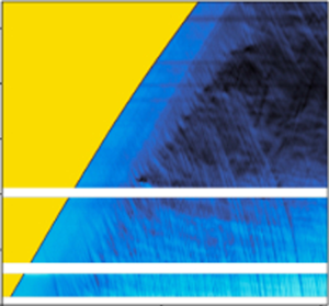
Example images from an experiment are shown in figure 3(a). A clearly defined finger initially forms and travels upwards, approximately centrally. At later times, a range of instabilities emerge behind the advancing finger front, resulting in progressive mixing across the pipe. Different variations will be discussed below in § 3. The scaled intensity  $I$ is interpreted as a depth-averaged concentration field. The concentration field is averaged across the pipe cross-section, to give an averaged concentration
 $\bar {\mathcal {C}}(\hat {z},\hat {t})$, as plotted in the inset of figure 3(b). The steep jump from
 $\bar {\mathcal {C}} \approx 0.2\ \text {to}\ \bar {\mathcal {C}} \approx 0.8$ in the inset indicates a sharp front is present between the two fluids. The spacing between the curves plotted is relatively constant, suggesting that the finger rises at a constant front velocity. To determine this velocity we replot
 $\bar {\mathcal {C}}({\hat {z},\hat {t}})$ against
 $\hat {z}/{\hat {t}}$, as shown in figure 3(b). The profiles of
 $\bar {\mathcal {C}}({\hat {z}/\hat {t}})$ collapse onto a single curve centred around the constant front velocity, here
 $5.7\ {\rm mm}\ {\rm s}^{-1}$.
Example results for an exchange flow experiment with  $At = 1.01\times 10^{-1}\text { and }m = 1.27\times 10^3$, defined later in (2.1) and (2.4). The physical parameters are from case 1, listed in table 1. (a) Evolution of the rising finger in the pipe at different times. (b) The concentration front obtained by averaging across the pipe radius at it passes through the pipe. The opacity of the concentration lines
 $\bar {\mathcal {C}}$ represents the time of the front. The lighter lines represent early times and as the front advances though space and time the lines darken to display this phenomenon the finger advancing. The larger figure in (b) shows the master curve for
 $\bar {\mathcal {C}}(\hat {z}/\hat {t},\hat {t})$ and the collapse onto a single front velocity. (c) The gap-averaged concentration
 $\bar {\mathcal {C}}(\hat {z},\hat {t})$ in the form of a spatio-temporal plot: yellow represents the upper viscoplastic fluid; light blue represents the less dense lower fluid.

The same effect can be visualised through a spatio-temporal plot of  $\bar {\mathcal {C}}({\hat {z},\hat {t}})$, as shown in figure 3(c). Here, the leading front of the finger is evident. The speed of the sharp front in figure 3(c) does slowly change in time as the finger progresses up the pipe. In order to make comparisons between our experiments in a consistent way, we calculate the speed,
 $\hat {V}_L$, of the advancing light fluid finger, as the front passes the height
 $250\ {\rm mm}$. We also extract a finger radius
 $\hat {r}_i$ at the same instant.
Since the pipe is closed, the upwards flow of light fluid is balanced by the downwards flow of heavy fluid, around the walls. From figure 3(c) (or from the images), we can see that there is an approximately uniform band of blue behind the front, representing the region where there is an exchange flow of well-defined fluid layers. Further below the front in figure 3(c), we then begin to see downwards moving streaks appear that represent surface waves associated with instability and subsequent mixing.
2.4. Dimensional analysis
Neglecting  $\hat {L}$, the
 $7$ dimensional parameters of table 1 can be arranged into 4 dimensionless groups. In general we may consider a dimensionless parameter that represents the density difference (or ratio), a viscosity ratio, a ratio of yield stress to buoyancy stress and a balance of buoyancy stresses with either viscous or inertial stresses. The latter balances lead to representative velocities that may also be used to scale
 $\hat {V}_L$. Thus, a dimensionless
 $V_L$ should be defined by at most 4 dimensionless groups, plus
 $n$. Evidently, different scalings bring out different features of the flow.
Regarding the density difference, we use the Atwood number
 \begin{equation} At = \frac{\hat{\rho}_H - \hat{\rho}_L}{(\hat{\rho}_H+\hat{\rho}_L)} \in [2.4 \times 10^{{-}2}, 1.13 \times 10^{{-}1}], \end{equation}
Debacq et al. studied exchange flows of iso-viscous miscible fluids in a similar size laboratory experiment, varying principally  $At$, using densified water as the working fluid (Debacq et al. Reference Debacq, Fanguet, Hulin, Salin and Perrin2001). For
 $At \ge 4 \times 10^{-3}$ they found that the fluids mixed fully across the pipe, resulting in a diffusive axial spreading. For
 $At \le 1.5 \times 10^{-4}$ the flows were non-diffusive. The transitions with
 $At$ depend, however, on the fluid viscosity, becoming less diffusive as the viscosity increases (Debacq et al. Reference Debacq, Fanguet, Hulin, Salin, Perrin and Hinch2003). Given our Atwood number range, we would expect a strongly diffusive regime if the upper fluid were water. However, the effective viscosity of the Carbopol solutions is very large and as we observe in figure 3(a), even late in the experiments and far behind the propagating finger, the mixing is not fully effective across the pipe.
The effects of viscosity on the regime transitions, and also pipe inclination were explored further by Séon et al. (Reference Séon, Hulin, Salin, Perrin and Hinch2005). Following the approach of Seon and co-authors, to understand the flow regimes we proceed to define inertial ( $\hat {V}_t$) and viscous velocity scales. The buoyancy–inertia balance (
 $\hat {\bar {\rho }} \hat {V}_t^2 \sim \Delta \hat {\rho } \hat {g} \hat {R}$) leads to
 $\hat {V}_t = \sqrt {2 At \hat {g}\hat {R}}$. Buoyancy–viscosity balances with either fluid lead to
 \begin{equation} \hat{V}_{v,L} = \frac{\Delta \hat{\rho} \hat{g} \hat{R}^2}{\hat{\mu}_L}, \quad \hat{V}_{v,H} = \left[\frac{\Delta \hat{\rho} \hat{g} \hat{R}}{\hat{\kappa}} \right]^{1/n} \hat{R}. \end{equation}
The ratio  $\hat {V}_{v,L}/\hat {V}_{t}$ defines a Reynolds number
 $Re_{t,L}$ relevant to
 $\hat {V}_t$ and the light fluid. We find
 $Re_{t,L} > 650$ for our experiments, which confirms that the lower fluid viscous stresses are largely irrelevant. Indeed,
 $\hat {V}_{v,L}$ is as much as 4 orders of magnitude more than the
 $\hat {V}_{L}$ that we measure. In contrast, on using the heavy fluid properties, we have
 \begin{equation} Re_{t,H} = \left[ \frac{\hat{V}_{v,H}}{\hat{V}_{t}} \right]^n = \frac{ \hat{\bar{\rho}} \hat{R} \hat{V}_{t} }{ \hat{\kappa} ( \hat{V}_{t}/\hat{R} )^{n-1}} \in [0.21,11.8] . \end{equation}
The transition from viscous-dominated exchange flows to inertia-dominated occurs at  $Re_t \gtrapprox 100$ for iso-viscous Newtonian fluids (Séon et al. Reference Séon, Hulin, Salin, Perrin and Hinch2005), suggesting that we remain firmly in a viscous regime for the heavy fluid. Thus, the picture emerging is of a buoyancy-driven flow in which the motions are principally resisted by viscous deformation of the thicker upper fluid.
When we have a structured finger we may develop better understanding of the upper fluid viscous stresses, within the wall layers for example, as we do later in § 3.3. Here, we deal only with bulk flow quantities. The speed  $\hat {V}_{v,L}$ can be used to define a strain rate and consequently an effective viscosity for the upper fluid. Using this, we may define a viscosity ratio (heavy to light) as follows:
 \begin{equation} m = \frac{ \hat{\kappa} \left( \hat{V}_{v,H}/\hat{R} \right)^{n-1}}{ \hat{\mu}_{L} } = \frac{\hat{V}_{v,L}}{\hat{V}_{v,H}}. \end{equation}
For larger values of  $\hat {V}_{v,H}$ the effective viscosity is reduced through shear thinning and the viscosity ratio above reduces. Nevertheless, for all experiments
 $m > 23$ and for most of our experiments
 $m$ is significantly larger. Figure 4 plots
 $Re_{t,H}$ vs
 $m$ for our experiments, showing a reduction in
 $m$ as the flows become progressively inertial. The flow regimes indicated in this figure are discussed later in § 3.2.4.
Overview of all experimental regimes in the  $Re_{t,H}$,
 $m$ plane: +, green designates experiments displaying helical finger regimes;
 $\blacklozenge$, red signifies fingers with a disconnected finger front;
 $\blacktriangle$, grey indicates experiments manifested a slug finger regime;
 $\times$, yellow shows experiments that result in no flows;
 $\bullet$, blue shows no-flow experiments conducted by Vogl et al. (Reference Vogl, Waldal, Sarmadi, Fershtman, Mitishita and Frigaard2022).

On measuring  $\hat {V}_{L}$, since the net flow on any cross-section is zero, the heavy fluid velocity is:
 $\hat {V}_{H} = \hat {V}_{L}\hat {r}_i^2/(1-\hat {r}_i^2)$, which is generally smaller than
 $\hat {V}_{L}$ for the observed
 $\hat {r}_i$. We use
 $\hat {V}_{H}$ to define
 \begin{equation} Re_{H} = \frac{ \hat{\bar{\rho}} \hat{R} \hat{V}_{H} }{ \hat{\kappa} ( \hat{V}_{H}/\hat{R} )^{n-1}} \in [0,12.3] . \end{equation}
Figure 5(a) plots  $Re_H$ vs
 $Re_{t,H}$ for our experiments. The two variables follow a trend of increasing inertia along which the observed flow regimes change sequentially. The transition between regimes is similar to that of figure 4 above, underscoring the relevance of the buoyancy viscous stress balance, with the heavy fluid. Figure 5(b) plots the analogous
 $Re_L$ vs
 $Re_{t,L}$, which shows a wide range of
 $Re_{t,L}\gtrapprox 600$ in each regime and is generally less coherent.
(a) Comparison of scaled heavy fluid Reynolds number  $Re_{t,H}$ and experimental Reynolds number
 $Re_H$. (b) Comparison of scaled light fluid Reynolds number
 $Re_{t,L}$ and experimental Reynolds number
 $Re_L$.

In the above analysis we have not discussed the role of the yield stress of the upper fluid. Briefly, the yield stress may act in 2 ways. First, the yield stress may prevent significant motion from occurring in the flow, beyond the initial disturbance of opening the gate valve. This is governed by the ratio of yield to buoyancy stress,  $Y$
 \begin{equation} Y = \frac{\hat{\tau}_y}{\Delta \hat{\rho}\hat{g}\hat{R}}, \end{equation}
known as the yield number. Secondly, when sustained motion occurs, it is often convenient to include the effects of the yield stress in comparison with those of the effective viscosity. This ratio is referred to as a Bingham number. Using a Bingham number instead of  $Y$ is simply a different choice of dimensionless groups, and is less relevant here where buoyancy drives the flow.
3. Results
We present our observations in 2 principal subsections. First, directly below we consider the loss of mechanical stability of the system, i.e. the transition from no flow to a sustained exchange flow. Secondly, we consider the different flows observed when a sustained exchange flow occurs.
3.1. No-flow experiments
The question of mechanical stability is deceptively simple. For a vertical pipe, a perfectly perpendicular (horizontal) interface generates no shear stresses: a hydrostatic solution exists. Thus, for any fluid with a finite yield stress, such interfaces should be statically stable. A linear perturbation from the horizontal interface induces linear deviatoric stresses, i.e. proportional to the destabilising buoyancy stress ( $\Delta \hat {\rho }\hat {g}\hat {R}$) and linear in amplitude of the perturbation. Thus, we can also expect the critical
 $Y$, needed to ensure static stability, will also be linear in the perturbation.
However, now the complexity manifests. Different interface orientations induce different shear stresses. Thus effectively, in order to guarantee stability, one requires an exhaustive examination of all interface configurations, to determine the level of deviatoric stresses induced. This is impractical, but configurations which destabilise and evolve into a sustained viscous exchange flow are of importance. One idea is to understand what yield number range allows such flows to occur. This approach is followed analytically and computationally by Frigaard (Reference Frigaard1998) and Frigaard & Scherzer (Reference Frigaard and Scherzer1998, Reference Frigaard and Scherzer2000), dealing with plane channel flow and pipe flow with different interface configurations. The chief idea is to develop a thin-film two-layer model for the exchange flow and then find conditions where there is no flow possible. Although these studies consider 2 Bingham fluids in exchange flow, for the limit of zero flow, all simple yield stress fluid models have the same limits. In Frigaard & Crawshaw (Reference Frigaard and Crawshaw1999) these results are combined with those for interfaces perpendicular to the pipe axis (the worst case in a horizontal pipe), to give estimates of critical yield numbers in pipes of varying inclination.
Consideration of different interface configurations is, however, necessary, as this aspect appears quite variable and sensitive in experimental observations. In inclined pipes, unsurprisingly a slump-like interface is the most common (Crawshaw & Frigaard Reference Crawshaw and Frigaard1999; Malekmohammadi et al. Reference Malekmohammadi, Naccache, Frigaard and Martinez2010). In vertical pipes, Varges et al. (Reference Varges, Fonseca, Costa, Naccache, de Souza Mendes and Pinho2018) placed Carbopol gels over less dense (vegetable or mineral) oil. The resulting exchange flow patterns observed included a ‘plug’ flow in which a central finger of (unyielded) Carbopol descended into the less dense oils, displacing them upwards along the wall. Plausibly here, fluid immiscibility may ensure that the aqueous Carbopol solution cannot wet the wall and hence descends centrally in the pipe. However, more recently, Longo et al. (Reference Longo, Chiapponi, Petrolo, Bosa and Di Federico2022) report experiments in which Carbopol solutions are placed below denser glycerol or honey, i.e. miscible. In these experiments the Carbopol finger was again observed to ascend centrally. In contrast, for all the experiments reported here: (a) it is the water that ascends into the Carbopol; (b) it does so centrally. In the earlier experiments of Vogl et al. (Reference Vogl, Waldal, Sarmadi, Fershtman, Mitishita and Frigaard2022), in the same apparatus, we also mostly observed the same phenomena but did observe a ‘side-by-side’ mode in 2 experiments, (effectively corresponding to the stratified slumping configurations of inclined pipe exchange flows). Why particular interface configurations are selected remains unsolved, i.e. beyond the influence of initial disturbances. An interesting study in this regard is that of Beckett et al. (Reference Beckett, Mader, Phillips, Rust and Witham2011), who considered vertical Newtonian exchange flows at very low Reynolds numbers and with carefully regulated initial conditions. They still, however, observed both concentric and side-by-side configurations developing.
The above discussion explains the reasons for considering a range of interface configurations in determining static stability. The bounds in Frigaard & Crawshaw (Reference Frigaard and Crawshaw1999) are determined for combinations of 2 yield stress fluids. For a single yield stress fluid flowing axially in a vertical pipe, the stability criterion corresponds to  $Y > Y_c = 0.6086$ for static stability of a side-to-side configuration (Frigaard & Scherzer Reference Frigaard and Scherzer2000). For the concentric interface configuration that we observe, in which the outer fluid has a yield stress, this reduces to
 $Y > Y_c = 0.5$ for static stability (Frigaard & Scherzer Reference Frigaard and Scherzer2000). However, it is worth noting that the concentric interface configuration in which the outer fluid has no yield stress, has no critical value of
 $Y$, i.e. the central flows observed by Varges et al. (Reference Varges, Fonseca, Costa, Naccache, de Souza Mendes and Pinho2018); Longo et al. (Reference Longo, Chiapponi, Petrolo, Bosa and Di Federico2022) are not prevented by the yield stress.
Thus, an effective  $Y = Y_{c,exp}$ should be determined from the actual experiments conducted, for the observed interfacial motions. Experiments from Crawshaw & Frigaard (Reference Crawshaw and Frigaard1999) and Frigaard & Crawshaw (Reference Frigaard and Crawshaw1999) are interesting in this regard. In these, a tube was half-filled with dense fluid, then light fluid added carefully on top (density stable). The tube was initially either vertical (perpendicular interface) or angled to give a slanted interface. To start the experiment the (closed) stable tube was inverted and placed at a desired inclination. It was then observed to see if the interface failed or not. This enabled
 $Y_c$ to be estimated for different angled interfaces. For a single yield stress fluid in a vertical pipe, it is found that
 $Y_{c,exp} \approx 0.2$ for an interface at
 $10^\circ$ from horizontal and
 $Y_{c,exp} \approx 0.3$ for an interface at
 $45^\circ$ from horizontal. Although this procedure does not directly disturb the (initially stable) interface, inversion of the tube imposes initial accelerations. For other experiments, such as Malekmohammadi et al. (Reference Malekmohammadi, Naccache, Frigaard and Martinez2010), Varges et al. (Reference Varges, Fonseca, Costa, Naccache, de Souza Mendes and Pinho2018), Longo et al. (Reference Longo, Chiapponi, Petrolo, Bosa and Di Federico2022) and Vogl et al. (Reference Vogl, Waldal, Sarmadi, Fershtman, Mitishita and Frigaard2022); and here, the experiment is initiated by opening a sliding gate valve, which also initiates motion. The size of this initial motion is not quantified and in our set-up the gate valve obscures the view of the initial interface. A different method could involve injection of the heavier fluid into the pipe, which creates an initial disturbance from the perspective of static stability. Thus,
 $Y_{c,exp}$ depends on the protocol adopted for placement of the fluids and any initial condition.
For the current experiments, in figure 6 we show a plot of  $Y$ against
 $Re_H$, for our data and the no-flow data of Vogl et al. (Reference Vogl, Waldal, Sarmadi, Fershtman, Mitishita and Frigaard2022), totalling twelve no flows. The results show that
 $Y_c = 0.5$ remains a valid but conservative estimate of the no-flow limit. We observed no flows well below this limit, with the lowest being
 $Y = 0.17$. A practical limit for our apparatus and protocols is
 $Y_{c,exp} \approx 0.2$. Generally speaking, our fluids have a high consistency and consequently high effective viscosities. This might mean that the initial disturbance is viscously damped before the interface can evolve to a sufficiently unstable configuration for a sustained exchange flow to develop when theoretically possibly.
Overview of all experimental results, classified in the  $(Re_H,Y)$ plane, to compare with the no-flow criteria established by Frigaard & Crawshaw (Reference Frigaard and Crawshaw1999). Two critical
 $Y$ values:
 $Y_c$,
 $Y_{c,exp}$ are marked: +, green designates experiments displaying helical finger regimes;
 $\blacklozenge$, red signifies fingers with a disconnected finger front;
 $\blacktriangle$, grey indicates experiments manifested a slug finger regime;
 $\times$, yellow shows experiments that result in no flow;
 $\bullet$, blue shows no-flow experiments conducted by Vogl et al. (Reference Vogl, Waldal, Sarmadi, Fershtman, Mitishita and Frigaard2022).

3.2. Sustained exchange flows
After the initial opening of the gate valve, many of our experiments evolve into a sustained flow. The initial transient close to the gate valve is not observable in our experiment, but we note that the time scales for viscous dissipation in the 2 fluids are quite different and this disparity may allow for the interface to evolve to a less stable configuration. We observe a long viscous finger or slug that initially rises centrally in the pipe. Figure 7 shows the variation of observed behaviours at fixed  $At$ as the yield stress (hence
 $Y$) is progressively reduced. The width of initial finger/slug decreases with
 $Y$. Each flow appears to become vulnerable to interfacial instabilities, behind the leading front. These instabilities can propagate as surface waves, even catching the front, (see figure 7b,c), and/or they grow in amplitude allowing the rising finger to detach into a slug; see figure 7(d–f). Helical asymmetries are commonly observed in the instabilities.
Sequence of experiments for cases 2–7 at  $At = 10^{-2}$, with decreasing
 $Y$, describing the evolution from a helical to a disconnected finger, ultimately transitioning to a slug-type flow. From (a–f),
 $Y = 1.88\times 10^{-1}, 1.32\times 10^{-1}, 6.31\times 10^{-2}, 8.23\times 10^{-3}$,
 $1.06\times 10^{-4}, 8.59\times 10^{-5}$. The times for each image are
 $\hat {t} = [0,86,173,259,346,432]\ {\rm s}$,
 $\hat {t} = [0,229,458,687,916,1145]\ {\rm s}$,
 $\hat {t} = [0,107,215,323,431,539]\ {\rm s}$,
 $\hat {t} = [0,26,53,79,106,132]\ {\rm s}$,
 $\hat {t} = [0,15,30,46,61,76]\ {\rm s}$,
 $\hat {t} = [0,9,18,27,36,45]\ {\rm s}$.

3.2.1. Helical finger
The helical finger was the most common flow type observed in our experiments. Figure 8 shows two experiments that illustrate this type of flow. The early time images of figure 8(a i,b i) show the finger penetrating as a centrally stable finger. The time scale of any initial inertia-dominated regime is very short as the interface elongates into a steady viscous-dominated finger. This steady finger regime is evident at early times of the spatio-temporal plot in figure 8(a ii,b ii), where we see a distinct sharp front persisting. The steady front velocity  $\hat {V}_L$ is measured in this part of the flow. This steady finger characterises the viscous-dominated phase of the helical finger and during this phase no instabilities are evident, either at the interface in the images or in the spatio-temporal plots.
Cases 8 and 9 illustrating the helical finger regime: (a i) represents an experiment with  $Re_H = 3.91\times 10^{-2}$,
 $Re/Fr^2 = 4.29\times 10^{-1}$,
 $Y = 5.92\times 10^{-2}$,
 $m = 6.22\times 10^2$ taken at different times
 $\hat {t}$ indicated under the image. (a ii) Shows the spatio-temporal plot
 $\bar {\mathcal {C}}$ with pure blue colour representing the light Newtonian fluid while yellow shows the heavy yield stress fluid and black displaying
 $\mathcal {C} = 0.5$. (b i) Shows another typical helical finger with
 $Re_H = 1.16\times 10^{-1}$,
 $Re/Fr^2= 2.29\times 10^{-1}$,
 $Y = 7.26\times 10^{-3}$,
 $m = 7.79\times 10^2$. (b ii) Shows the spatio-temporal
 $\bar {\mathcal {C}}$ of the experiment in (b i).

The upwards flow of the finger displaces the heavy fluid downwards, which requires the heavy fluid to yield at the wall. At the interface  $\hat {r} = \hat {r}_i$, things are less clear. Considered as a shear flow, the heavy fluid layer may be yielded at the interface or not, depending on
 $\hat {r}_i$. However, the flow also develops slowly in
 $\hat {z}$, which allows for extensional deformations. In either case the effective viscosity of the descending heavy fluid layer is large (typically
 $0.2\unicode{x2013}10$ Pa s, based on
 $m$). Thus, the interfacial instabilities that appear do so on a slow viscous time scale, controlled by the heavy fluid. In the spatio-temporal plots, we begin to see downwards streaks that correspond to these interfacial wave speeds. The initial growth/propagation appears to be helical, but as the amplitudes grow, any symmetry is lost. Tracing horizontally in the spatio-temporal plots, we see that at the lower
 $\hat {z}$, there is a significant delay before an instability is observed. However, higher in the pipe the interfacial waves occur progressively close to the front as it passes. It is unclear why this happens.
Behind the advancing finger at later times, interfacial yielding and buoyancy-driven deformation causes 3-D flow features to emerge between the two fluids. This results in some advective mixing of the two fluids, but we still observe distinct fluid regions even late in the flow. The growth of interfacial waves of the heavy fluid seems to cut into the conduit of clear lower fluid, making any pathway more tortuous. The larger surface waves descend below the gate valve into the light fluid region, where they eventually break off from the wall layer. Experiments from Vogl et al. (Reference Vogl, Waldal, Sarmadi, Fershtman, Mitishita and Frigaard2022) show the descent of detached viscoplastic droplets, the larger of which are jellyfish-shaped. These features were also observed in our experiments.
3.2.2. Disconnected finger
The initiation of this regime is similar to the helical finger regime. However, in the disconnected finger regime detachment from the bulk flow is observed; see figure 9(a i,b i) for examples. The detached finger proceeds upwards at speed approximately  $\hat {V}_L$, maintaining a near-constant length during the experimental time. Behind the finger, there is some advective mixing driven by buoyancy and we see some degradation of the rear of the finger.
Disconnected finger regime illustrated by cases 10 and 11: (a i) represents a disconnected finger characterised by  $Re_H = 4.92\times 10^{-2}$,
 $Y = 4.75\times 10^{-5}$,
 $Re/Fr^2 = 1.01\times 10^{-1}$,
 $m = 1.27\times 10^3$ taken at different times
 $\hat {t}$, as indicated under the image. (a ii) Shows the spatio-temporal plot with a gap-averaged concentration
 $\bar {\mathcal {C}}$ with pure blue colour representing the light Newtonian fluid while yellow shows the heavy yield stress fluid and black displaying
 $\bar {\mathcal {C}} = 0.5$. (b i) Displays another disconnected finger with
 $Re_H = 1.49$,
 $Re/Fr^2=3.93\times 10^{-1}$,
 $Y = 1.06\times 10^{-2}$,
 $m = 1.30\times 10^2$. (b ii) Shows the spatio-temporal plot
 $\bar {\mathcal {C}}$ of the disconnected finger.

The most striking features are seen in the spatio-temporal plots of figure 9(a ii,b ii). It seems that the transition at the end of the finger is relatively sharp and the detachment of the finger breaks continuity with the bulk of the lower fluid. Below the rising blue band (detached finger) in these plots, we see emerge a brown triangular region denoting the mixed  $\bar {\mathcal {C}}$. Notable here is that where the fluids mix the most, the downwards and upwards streaks/contours are significantly shallower than the advancing front speed (or the earlier descending waves). The finger detachment appears to result in a stabilising buffer region in which fluid motions are significantly reduced.
3.2.3. Slug flow
The slug flow regime was observed in the more inertial regimes (larger  $Re_H$). Figure 10(a i,b i) shows examples of the slug propagation. The main difference with the disconnected finger regime is that the initial stable finger does not form and instead a detached slug or droplet rises. We distinguish these from the detached finger also by the shorter observed lengths (a few diameters). This may of course be simply part of continuous variation in the detachment process as the Carbopol concentration is reduced. The spatio-temporal plots in figure 10(a ii,b ii) show that the front speed decreases throughout the experiment. In figure 10(a) the slug detaches completely from the lower fluid, although we do see a secondary front moving upwards through a thin helical path. As previously, the brown regions of intermediate
 $\bar {\mathcal {C}}$ in the spatio-temporal plots have shallower contours, indicating stabilisation. Reasons for the decline in velocity are unclear. In case 12 (figure 10a) the slug is detached completely. Possibly the volume decreases via miscibility at the edges. Behind the slug, there is an exchange flow region that widens and mixes laterally with time, presumably reducing the driving force for the motion. The same mechanisms may be present in case 13 (figure 10b).
Slug regime illustrated by cases 12 and 13: (a i) represents an experiment with  $Re_H = 1.34\times 10^{-1}$,
 $Re/Fr^2 = 2.84\times 10^{-1}$,
 $Y = 5.09\times 10^{-2}$,
 $m = 5.65\times 10^2$ taken at different time
 $\hat {t}$, as indicated under the image. (a ii) Shows the spatio-temporal plot of the gap-averaged concentration
 $\bar {\mathcal {C}}$ with pure blue colour representing the light Newtonian fluid while yellow shows the heavy yield stress fluid and black displaying
 $\bar {\mathcal {C}} = 0.5$. (b i) Displays a slug with
 $Re_H = 1.23\times 10^1$,
 $Re/Fr^2 = 3.01\times 10^{-1}$,
 $Y = 8.59\times 10^{-5}$,
 $m =3.20\times 10^1$. (b ii) The spatio-temporal plot of the gap-averaged concentration
 $\bar {\mathcal {C}}$ vs time
 $\hat {t}$.

3.2.4. Classification of flow regimes
The above classification is based on experimental observation. To quantify our results and gain insight into the physical cause of the transitions, we plot our experiments against some of the dimensionless parameters derived in § 2.4. Figure 11(a) shows our experiments, as the inertial stresses increase. This is captured in both  $Re_H$ and in
 $Fr_H = \hat {V}_H / \hat {V}_t$. The regimes are identified by the symbol shape and the symbol colour scale gives the range of
 $V_H$. As the flow becomes progressively inertial, we move from helical finger to disconnected to slug. Figure 11(b) illustrates the change in effective viscosity ratio through the flow regimes. It also presents the range of observed
 $r_i$, which is quite limited. In general the larger
 $r_i$ are associated with the more inertial regimes.
Classification of the flowing experiments into the different regimes. (a) Average velocity  $V_H$ (colour map) plotted in the
 $(Fr_H,Re_H)$-plane. (b) Value of
 $r_i$ (colour map) plotted in the
 $(m,Re_H)$-plane. Symbols: + denotes helical finger;
 $\blacklozenge$ denotes disconnected finger;
 $\blacktriangle$ denotes slug finger regime.

As there is no imposed flow rate, the driving force for the (increasingly inertial) flow regimes must come from buoyancy. The combination  $Re_H/Fr_H^2$ can be unravelled to give
 \begin{equation} \frac{Re_H}{Fr_H^2} = \frac{\Delta \hat{\rho} \hat{g} \hat{R}}{\hat{\kappa} \left( \hat{V}_{H}/\hat{R} \right)^{n}} , \end{equation}
which clearly represents the balance of buoyancy with the viscous stresses of the heavy fluid. Figure 12 shows the regime transitions in the  $(Re_H,Re_H/Fr_H^2)$ plane. We see that the flows all occur with
 $Re_H/Fr_H^2 \sim 1$ and the transitions away from the helical finger regime occur at a critical
 $Re_H = Re_c \approx 1$.
Flowing regime transitions in the  $(Re_H,Re_H/Fr_H^2)$ plane. Symbols: +, green denotes helical finger;
 $\blacklozenge$, red denotes disconnected finger;
 $\blacktriangle$, grey denotes slug finger regime.

3.3. Lubrication model and analysis
Using standard scaling methods we can derive a reduced model, relevant to the stage of the experiments when the velocity field is approximately aligned with the axis of the tube and the interface is finger-like. We assume an axisymmetric flow with a buoyant finger of the light fluid rising upwards, displacing the lower fluid downwards. Following scaling arguments as in Frigaard (Reference Frigaard1998) and Frigaard & Scherzer (Reference Frigaard and Scherzer1998), we find that to leading order the velocity is in the axial direction, denoted  $\hat {w}(\hat {r})$, the pressure does not vary across the pipe and the axial momentum balance is
 \begin{equation} 0 ={-}\frac{\partial \hat{p}}{\partial \hat{z}} + \frac{1}{\hat{r}} \frac{\partial }{\partial \hat{r}} [ \hat{r} \hat{\tau}_{k,rz} ] - \hat{\rho}_{k}\hat{g}, \quad k = H,L. \end{equation}
Here, for  $\hat {r} \in [0,\hat {r}_i)$ we have
 $k=L$ and we are in the light fluid finger. For
 $\hat {r} \in (\hat {r}_i,\hat {R}]$ we have
 $k=H$ and are in the heavy fluid.
Having simplified the mathematical description above, we now adopt scalings based on the heavy fluid buoyancy–viscous stress balance:  $\Delta \hat {\rho } \hat {g} \hat {R} = \hat {\kappa } (\hat {V}_{v,H}/\hat {R} )^n$. The velocity
 $\hat {w}(\hat {r})$ is scaled with
 $\hat {V}_{v,H}$, the lengths with
 $\hat {R}$ and the stresses with
 $\Delta \hat {\rho } \hat {g} \hat {R}$. We also define
 $f$ as the scaled modified pressure gradient in the light fluid
 \begin{equation} f \Delta \hat{\rho} \hat{g} \hat{R} ={-}\frac{\partial \hat{p}}{\partial \hat{z}} - \hat{\rho}_{L}\hat{g} . \end{equation}
The dimensionless momentum balances are
 $$\begin{gather} \frac{1}{r} \frac{{\rm d}}{{\rm d}r}(r\tau_{L}) ={-}f,\quad \Rightarrow\quad \tau_{L} ={-} \frac{fr}{2}, \quad r \in (0,r_{i}) , \end{gather}$$
 $$\begin{gather}\frac{1}{r} \frac{{\rm d}}{{\rm d}r}(r\tau_{H}) = 1 -f, \quad \Rightarrow \quad \tau_{H} = \frac{1}{2}\left((1-f)r - \frac{r_i^{2}}{r}\right),\quad r \in (r_{i},1) . \end{gather}$$
Here,  $\tau _k$ is the leading-order shear stress in fluid
 $k$:
 $\tau _k = \tau _{k,rz}$, defined via constitutive laws below. The following conditions are satisfied as symmetry, interface and boundary conditions:
 $$\begin{gather} \tau_{L}(0) = 0, \end{gather}$$
 $$\begin{gather}w(r_i^-) = w(r_i^+), \end{gather}$$
 $$\begin{gather}\tau_{L}(r_i^-) = \tau_{H}(r_i^+), \end{gather}$$
 $$\begin{gather}w(1) = 0. \end{gather}$$
Flows of this type have been studied in Frigaard & Scherzer (Reference Frigaard and Scherzer1998, Reference Frigaard and Scherzer2000). In general, (3.4)–(3.9), can be solved to give a unique axial velocity  $w = w(r;r_i,f)$, which depends on the interface position and on
 $f$, (plus of course the dimensionless rheological parameters
 $m,Y,n$).
For the exchange flow configuration, the ascending upwards finger is balanced by the descending heavy fluid near the walls. Thus, we expect that  $w$ is maximal at the centre, decreasing with
 $r$ to the interface. In order for the fluid near the wall to be pushed downwards, we would also expect that
 $w(r)$ is increasing as
 $r \to 1$. These expectations lead to the intuitive notion that
 $f \in (0,1)$, i.e. fluid
 $L$ is pushed upwards and fluid
 $H$ downwards. To make more precise the notion of balance, suppose that we have calculated the velocity,
 $w(r;r_i,f)$. We then integrate across each layer
 \begin{equation} Q_{L}(r_i,f) = 2 {\rm \pi}\int_0^{r_i} r w(r;r_i,f)\,{\rm d}r,\quad Q_{H}(r_i,f) = 2 {\rm \pi}\int_{r_i}^1 r w(r;r_i,f)\,{\rm d}r. \end{equation}
The results from Frigaard & Scherzer (Reference Frigaard and Scherzer1998, Reference Frigaard and Scherzer2000) can be applied. For example, it is known that the total flow rate  $Q = Q_L + Q_H$ increases monotonically with
 $f$, which means we can always find a value of
 $f$ for which
 $Q = 0$, i.e. an exchange flow. If neither fluid has a yield stress then the monotonicity of
 $Q(f)$ is strict and there will be a single value of
 $f \in (0,1)$ for which
 $Q=0$. When fluid
 $H$ has a yield stress it may become stuck to the outer wall, over some range of
 $f$. This can mean that a range of values of
 $f$ allow
 $Q = 0$. Lastly, in general
 $Q_L$ increases with
 $f$ and
 $Q_H$ decreases with
 $f$.
Moving now to the specific exchange flows relevant to our experiments, the inner fluid is Newtonian and the outer fluid can be described as a Herschel–Bulkley fluid. The scaled constitutive laws are
 \begin{gather} \tau_{L} = \frac{1}{m}\frac{{\rm d}w}{{\rm d}r}, \end{gather}
 \begin{gather} \left. \begin{gathered}
\tau_{H} =\left( \displaystyle{\left|\frac{{\rm d}w}{{\rm
d}r}\right|^{n-1}}
+\frac{Y}{\displaystyle{\left|\dfrac{{\rm d}w}{{\rm
d}r}\right|} } \right) \displaystyle{\frac{{\rm d}w}{{\rm
d}r}} \quad\Leftrightarrow\quad |\tau_{H}| > Y,\\
\displaystyle{\left|\frac{{\rm d}w}{{\rm d}r}\right|} = 0
\quad \Leftrightarrow\quad |\tau_{H}| \le Y.\end{gathered}
\right\} \end{gather}
Here, the viscosity ratio  $m$ is defined in (2.4) and the yield number is defined in (2.6).
The exchange flow solution can be calculated iteratively for each  $r_i$, by using e.g. the bisection method, to find an
 $f(r_i)$ for which
 $Q_L + Q_H = 0$. We therefore assume that we have found
 $[w(r;r_i,f),f(r_i)]$ for each
 $r_i \in [0,1]$. Figure 13(a) shows a typical example of the variations in
 $Q_L(r_i)$ and
 $Q_H(r_i)$, computed for
 $(m,Y,n) = (x,Y,Z)$. These functions approach zero as
 $r_i \to 0$, and also typically
 $Q_L = Q_H = 0$ for a band of
 $r_i$ close to
 $r_i = 1$, provided that fluid
 $H$ has a yield stress.
(a) An example of  $Q_L(r_i)$ and
 $Q_H(r_i)$, computed for
 $(m,Y,n) = (5.65\times 10^2,5.09\times 10^{-2},0.52)$. (b) The dimensionless interfacial radius
 $r_i$, plotted against
 $Y$ for our experiments, compared with the critical
 $Y_c(r_i)$ (dashed line).

For fixed fluid properties, having computed  $Q_L(r_i)$, the interface evolves according to
 \begin{equation} \frac{\partial}{\partial t} [{\rm \pi} r_i^2] + \frac{\partial}{\partial z}Q_L(r_i) = 0. \end{equation}
We do not solve (3.13), as it is well known that the lubrication model on its own does not predict the finger width, which is selected in the 2-D region at its tip.
3.3.1. Stress variations in the exchange flows
From the solution, for any given  $f$ the interfacial stress
 $\tau _i$ and the wall shear stress
 $\tau _w$, are computed from (3.4)
 \begin{equation} \tau_i ={-} \frac{fr_i}{2},\quad \tau_w = \frac{1}{2}\left(1-f - r_i^2\right). \end{equation}
It is not hard to see that, in order to have a non-trivial velocity, the velocity must increase as it approaches the wall at  $r=1$. This requires that
 $\tau _w > Y$. Therefore, a necessary condition to flow is that
 \begin{equation} \frac{1 - f - r_i^2 }{2} > Y, \quad \Rightarrow\quad f < 1 - r_i^2 - 2 Y = f_{max}. \end{equation}
Because also  $f_{max} \le 1$, we see that there is a critical yield number
 $Y_c(r_i) = (1-r_i^2)/2$ above which there can be no flow in our lubrication model. At
 $r_i = 0$ we see that
 $Y \ge 0.5$ is sufficient to prevent all non-zero flows. Figure 13(b) compares this critical
 $Y_c(r_i)$ with the experimental values of
 $Y$ and
 $r_i$. We see a clear demarcation of our experiments, above and below
 $Y_c(r_i)$. For experiments that do not flow, we simply take
 $r_i=1$. For the sustained exchange flows, as commented before, these are limited to
 $Y < Y_{c,exp} \approx 0.2$ for our experimental protocols.
Since we have also measured the interface radius  $r_i$ of the initial finger/slug that rises centrally in our experiments, we can compute
 $f$,
 $\tau _i$ and
 $\tau _w$ for each experiment. Figure 14(a) plots the excess wall shear stress
 $\tau _w - Y$, against
 $Y$. This confirms that the transition from no-flow to flow coincides with
 $\tau _w = Y$, as should be the case.
(a) Dimensionless excess wall shear stress  $\tau _w - Y$, plotted against
 $Y$. (b) Excess interfacial stress
 $Y + \tau _i$ plotted against
 $\tau _i$. The colour map displays the intensity of the Froude number
 $V_H/V_t$.

Figure 14(b) plots the excess interfacial stress  $Y + \tau _i$ against
 $\tau _i$ for our experiments. We observe that the transition through the observed regimes (helical finger
 $\rightarrow$ disconnected finger
 $\rightarrow$ slug) appears to be associated with
 $Y + \tau _i$ passing through zero. The more inertial regimes and those for which the finger/slug disconnects early correspond to those closer to yielding at the interface. The helical finger regime appears to be found exclusively with
 $Y + \tau _i > 0$. In other words, helical finger regimes corresponded to an unyielded plug at the interface. As it is simple to check this condition for the lubrication model, this could be used predictively to state whether a helical finger of given radius may be found.
The relevance of  $\tau _i = -Y$ becomes clearer if we consider qualitatively the type of velocity profile found in the sustained exchange flows. Fluid
 $L$ is Newtonian, the stress is linear, the velocity in
 $[0,r_i)$ is parabolic and we always have
 $\tau _i < 0$. The outer fluid may be yielded or unyielded at the interface, but must yield at the wall in order for there to be a flow. When
 $|\tau _i| \le Y$, the fluid is unyielded at the interface, which we define as a type I solution. Alternatively, the fluid may be yielded,
 $\tau _i < -Y$, which we define as type II. Figure 15 shows these two types of fluid velocity profile and the associated shear stress variations.
Schematic illustration of type I and type II velocity profiles, and associated stresses in an axisymmetric geometry. Blue indicates Newtonian fluid and red indicates viscoplastic.

The change in flow type may explain the persistence of the helical fingers until late in our experiments, whereas instabilities for the other regimes grew visibly earlier. The type I solutions are part of a family of possible stable viscoplastically lubricated solutions. Frigaard (Reference Frigaard2001) showed that retaining an unyielded plug at the interface of a multilayer viscoplastic flow could eliminate the possibility of linear interfacial instabilities. Remarkably, such flows can also be nonlinearly stable (Moyers-Gonzalez, Frigaard & Nouar Reference Moyers-Gonzalez, Frigaard and Nouar2004) and are realisable experimentally (Huen, Frigaard & Martinez Reference Huen, Frigaard and Martinez2007). The flows of Moyers-Gonzalez et al. (Reference Moyers-Gonzalez, Frigaard and Nouar2004) and Huen et al. (Reference Huen, Frigaard and Martinez2007) were, however, isodense and pumped co-currently. The set-up here involves counter-current flow and is driven by buoyancy. Although the arguments of Frigaard (Reference Frigaard2001) should apply to linear perturbations of an unyielded interface, as the interface elongates in our experiments we develop long layers of fluids of different density within which the neglected stress components may become significant. For example, extensional stresses arise in slowly developing thin-film flows of yield stress fluids, resulting in a pseudo-plug region within which the stress is asymptotically just above the yield stress (Balmforth & Craster Reference Balmforth and Craster1999). Certainly there is no obvious stabilising influence for our layered flows once the plug yields.
3.3.2. Comparisons with the exchange flows experiments
Further comparisons can be made directly with the experiments. Having found the exchange flow solution  $[w(r;r_i,f),f(r_i)]$, the net flow rate is
 \begin{equation} Q = Q_L + Q_H ={-} {\rm \pi}\int_{0}^{r_i} r^{2} \frac{{\rm d}w}{{\rm d}r}\,{\rm d}r - {\rm \pi}\int_{r_i}^1 r^{2} \frac{{\rm d}w}{{\rm d}r}\,{\rm d}r = 0. \end{equation}
Thus,  $Q_H = -Q_L$. The flux in fluid
 $L$ is given by
 \begin{equation} Q_{L} = {\rm \pi}r_i^{2}w(r_i) + {\rm \pi}\frac{m fr_i^{4}}{8} , \end{equation}
where  $w(r_i)$ is the velocity at the interface and can be found by integrating from the wall
 \begin{equation} w(r_i) = \int_{1}^{r_i} \frac{{\rm d}w}{{\rm d}r}\,{\rm d}r ={-} \int_{r_i}^1 \mathrm{sgn}(\tau_H(r)) \left( |\tau_H(r)| - Y \right)_+^{1/n}\,{\rm d}r , \end{equation}
where  $( {\cdot } )_+$ denotes the positive part. Similarly,
 $Q_H$ can be directly calculated
 \begin{equation} Q_{H} ={-} {\rm \pi}r_i^{2}w(r_i) + {\rm \pi}\int_{r_i}^1 r^{2} \mathrm{sgn}(\tau_H(r)) \left( |\tau_H(r)| - Y \right)_+^{1/n}\,{\rm d}r. \end{equation}
The mean velocity in the light and heavy fluids:  $\bar {V}_L$ and
 $\bar {V}_H$ are defined by
 \begin{equation} \bar{V}_L = \frac{Q_L}{{\rm \pi} r_i^{2}},\quad \bar{V}_H = \frac{-Q_H}{{\rm \pi} (1-r_i^{2})} = \frac{r_i^{2}}{1-r_i^{2}} \bar{V}_L . \end{equation}
The above may be compared with our experimental values. However, in the experiments we measure both  $\hat {V}_L$ and
 $\hat {r}_i$. Consequently, for comparison we take the measured
 $\hat {r}_i$, scale with
 $\hat {R}$ and compute
 $\bar {V}_H(r_i)$, as above, to compare with the experimental
 $\hat {V}_H$, also scaled with
 $\hat {V}_{v,H}$. Figure 16(a) shows 3 examples of this comparison. We also plot a representative error bar in
 $r_i$, noting that the observed
 $r_i$ values in our experiments are typically in the range of
 $r_i$ where
 $\bar {V}_H(r_i)$ is decreasing to zero. The observed and computed velocities are comparable. This is repeated with the dimensional velocities in figure 16(b), for all flowing experimental values, compared with computations using the measured
 $\hat {r}_i$. We see that the comparison is reasonable for the helical and disconnected regimes, but diverge for the slug regimes. This suggests that the longer near-parallel flows with approximately axisymmetric fingers (helical and disconnected regimes) are represented by the viscous shear flow vs buoyancy balance of our model. The slug flows likely represent a transition to a regime in which inertia–buoyancy is the more relevant balance. Additionally, in the slug flow regime some of the scaling arguments that underly the lubrication approximation are less valid.
(a) Model velocity  $\bar {V}_H(r_i)$ (lines) compared with experimental
 $V_H$ and
 $r_i$ for 3 examples. Error bars in are
 $r_i \pm 0.02$: (—, green) represents viscoplastic rheology
 $\hat {\rho }_H = 1200\ \textrm {kg}\ \textrm {m}^{-3}$,
 $\hat {\rho }_L = 1000\ \textrm {kg}\ \textrm {m}^{-3}$,
 $\hat {\tau }_{Y,H} = 0.579\ \textrm {Pa}$,
 $\hat {\kappa }_H = 8.003\ \textrm {Pa}\ \textrm {s}^n$,
 $n = 0.51$; (—, yellow) represents viscoplastic rheology
 $\hat {\rho }_H = 1125\ \textrm {kg}\ \textrm {m}^{-3}$,
 $\hat {\rho }_L = 1000\ \textrm {kg}\ \textrm {m}^{-3}$,
 $\hat {\tau }_{Y,H} = 0.001$ Pa,
 $\hat {\kappa }_H = 0.224\ \textrm {Pa}\ \textrm {s}^n$,
 $n = 0.67$; (—, blue) represents viscoplastic rheology
 $\hat {\rho }_H = 1150\ \textrm {kg}\ \textrm {m}^{-3}$,
 $\hat {\rho }_L = 1000\ \textrm {kg}\ \textrm {m}^{-3}$,
 $\hat {\tau }_{Y,H} = 0.436$ Pa,
 $\hat {\kappa }_H = 3.06\ \textrm {Pa}\ \textrm {s}^n$,
 $n = 0.52$. (b) Predicted velocity
 $\bar {V}_H$ plotted against the corresponding experimental velocity, dashed lines indicate
 $\pm 15\,\%$ error range.

3.4. Energy analysis
In our analysis and flow classification, it is curious that in all cases the initial (viscous) finger appears unable to persist in a stable state over long times. Although the experimental finger velocities  $V_L$ (and radii) compare reasonably with those computed from the lubrication model (figure 16b), it is well known that the lubrication model on its own is not predictive of the actual finger width observed.
In Longo et al. (Reference Longo, Chiapponi, Petrolo, Bosa and Di Federico2022) the authors develop an energy method, based on the work of Picchi, Suckale & Battiato (Reference Picchi, Suckale and Battiato2020) that was constructed for a Newtonian Taylor drop/slug. This method considers the energy balance for an idealised rising cylinder of core fluid, balanced with an annulus of descending fluid. Although the number of data points in Longo et al. (Reference Longo, Chiapponi, Petrolo, Bosa and Di Federico2022) is quite limited, the authors show a reasonable match between experimental rise velocities and those predicted as the asymptotic steady-state interface radius of their analysis.
In terms of our variables, the same energy balances as made in Longo et al. (Reference Longo, Chiapponi, Petrolo, Bosa and Di Federico2022) lead to the following evolution equation for the finger radius  $r_i(t)$:
 \begin{equation} t\frac{{\rm d} r_i}{{\rm d}t} = \displaystyle{ \frac{ \mathcal{P}_t(r_i) - \mathcal{D}(r_i) }{ \dfrac{{\rm d}}{{\rm d} r_i} \left[ Q_L^2(r_i) \dfrac{2r_i^2-1}{2{\rm \pi} r_i^2 (1 - r_i^2)} \right] } }, \end{equation}
where
 \begin{equation} \mathcal{P}_t(r_i) = Q_L^2(r_i) \frac{1-2r_i^2}{{\rm \pi} r_i^2 (1 - r_i^2)}, \end{equation}
where  $Q_L(r_i)$ is calculated as in the lubrication model and where
 $\mathcal {D}(r_i)$ represents the rate of dissipation, given here by
 \begin{equation} \mathcal{D}(r_i) = 2{\rm \pi} (\bar{V}_L+\bar{V}_H) \left( \frac{1}{m}\int_0^{r_i}r\left| \frac{{\rm d}w}{{\rm d}r}\right|^2\,{\rm d}r + \int_{r_i}^1 r\left| \frac{{\rm d}w}{{\rm d}r}\right|^{n+1} + rY\left| \frac{{\rm d}w}{{\rm d}r}\right|\,{\rm d}r \right). \end{equation}
The first term in (3.21) has a zero at  $r_i = 1/\sqrt {2}$. A small dissipation shifts this zero slightly. This zero represents an equilibrium solution of (3.21), which can be interpreted as an autonomous first-order differential equation for
 $r_i = r_i(\ln t)$. Longo et al. (Reference Longo, Chiapponi, Petrolo, Bosa and Di Federico2022) show that this equilibrium point is stable, and hence use this as the prediction for the asymptotic
 $r_i$.
We have followed the same procedure as Longo et al. (Reference Longo, Chiapponi, Petrolo, Bosa and Di Federico2022), but find no equilibrium points for the parameters that coincide with our experiments! While this may appear strange, note that in contrast to Longo et al. (Reference Longo, Chiapponi, Petrolo, Bosa and Di Federico2022) we have always found the less viscous Newtonian fluid to rise centrally in our experiments while the yield stress fluid descends near the walls. In figure 17 we show plots of the functions in (3.21), for one of our experiments. In the mid-range of  $r_i$ that we observe, the right-hand side of (3.21) is generally negative. This is because the dissipation rate dominates the first term of the numerator (related to the time derivative of the potential energy). The contrast with Longo et al. (Reference Longo, Chiapponi, Petrolo, Bosa and Di Federico2022) is then intuitive. For our fluids to flow, the outer more viscous fluid must yield at the wall. Thus, the most viscous fluid is deformed and occupies a larger area than if the fluids were reversed. Indeed, feasible exchange flow configurations with the Newtonian fluid on the outside include that with the inner fluid entirely unyielded, which has no contribution to the dissipation rate (Frigaard & Scherzer Reference Frigaard and Scherzer1998).
Examples from the energy analysis with:  $\hat {\rho }_H = 1100\ \textrm {kg}\ \textrm {m}^{-3}$,
 $\hat {\rho }_L = 1000\ \textrm {kg}\ \textrm {m}^{-3}$,
 $\hat {\tau }_{Y,H} = 0.232$ Pa,
 $\hat {\kappa }_H = 0.947$ Pa s
 $^n$,
 $n = 0.49$. (a) Variation in
 $Q_L$ (black),
 $\bar {V}_L$ (red),
 $\bar {V}_H$ (blue), with
 $r_i$. (b) Variation in
 $\mathcal {D}(r_i)$ (red) and
 $\mathcal {P}_t(r_i)$ (green), together with the numerator of (3.21) in black.

4. Discussion and conclusions
We have presented the results of a series of 40–50 experiments in which a denser yield stress fluid is positioned above water in a vertical circular pipe. The fluids are miscible and in the absence of any yield stress there is no static equilibrium. In contrast, with a yield stress there are many static equilibria, governed only by the configuration of the interface between the fluids and the yield number  $Y$. In our experiments the initial interface is horizontal, perpendicular to the pipe, which is statically stable for any
 $Y>0$. However, there is an initial disturbance due to opening of the gate valve separating the two fluids, which both induces stresses and disturbs the interface. Our results separate into two: those that flow and those where the initial disturbance decays and remain static in this mechanically unstable configuration. We find that there are no flowing (i.e. unstable) configurations with
 $Y > Y_{c,exp} = 0.2$. For the unstable configurations, the initial development of the front between fluids results in an approximately central finger of the water moving upwards through the Carbopol, which is displaced downwards around the walls. Fully developed core–annular exchange flows of this type cannot evolve for
 $Y \ge Y_c = 0.5$. Our no-flow results are consistent with both earlier experiments and theoretical understanding (Frigaard & Crawshaw Reference Frigaard and Crawshaw1999).
The flowing experiments have been further classified according to the behaviour of the initial central front. A long well-defined rising central finger may evolve, which either tends to destabilise slowly late in the experiment (helical finger), or can completely disconnect from the lower fluid (disconnected finger). Alternatively, the finger breaks and detaches very early in the experiment (slug). The transition through the regimes follows an increase in  $Re_H$ and decrease in
 $Y$ (figure 6), or decrease in
 $m$ (figure 11b). The more viscous helical finger regime is found for
 $Re_H \lessapprox Re_c = 1$. In other words, the flows become increasing inertial, noting that only buoyancy drives the flow.
Both  $m$ and
 $Y$ contribute to an effective viscosity ratio between the fluids, when flowing. At the typical shear rates of the experiments, the effective viscosity of the Carbopol dominates that of the water. Regardless of regime, the viscosity of the Carbopol plays a key role in balancing the driving buoyancy. This is captured in the balance
 $Re_H/Fr_H^2$, as illustrated in figure 12.
For the regimes where a long finger (or slug) evolves, it is reasonable to consider the flow at the sides of the finger to be close to one-dimensional. This leads to the lubrication (thin-film) model developed in § 3.3. Although such models give reasonable agreement with observed motions (figure 16b), these are simply based on the 1-D momentum balance and are not fully predictive. The 1-D model is useful in understanding the type of velocity profile around the rising finger. We see that helical fingers are associated with interfacial stresses lying below the yield stress ( $|\tau _i| < Y$) and type 1 velocities, whereas disconnected fingers and slug regimes correspond to type 2 velocities (see figure 15), with
 $|\tau _i| > Y$; see figure 14(b).
The observation that disconnected finger and slug regimes both correspond to core–annular regimes with a yielded interface is notable. Based on linear stability studies of multi-layer flow one expect that the configuration with the more viscous fluid near the wall will be unstable (Joseph & Renardy Reference Joseph and Renardy1992). Indeed for many situations studied this configuration is absolutely convectively unstable (d ’Olce et al. Reference d ’Olce, Martin, Rakotomala, Salin and Talon2009; Selvam et al. Reference Selvam, Talon, Lesshafft and Meiburg2009). Considering the effective viscosity of the yielded Carbopol near the interface, compared with that of water, we may interpret our flows as falling into this category.
The dichotomy between stable core–annular flows with yield stress vs unstable purely viscous flows has been noted and observed before. For example, in displacement flows of (viscous, shear-thinning) xanthan solutions with density-matched water, Gabard (Reference Gabard2001); Gabard & Hulin (Reference Gabard and Hulin2003) found an initially uniform central finger that only destabilised much later in their experiments. Displacing Carbopol (with a yield stress) did not destabilise. Some of our late stage destabilising fingers are reminiscent of those in Gabard (Reference Gabard2001) and also helical modes are commonplace in the Newtonian–Newtonian literature, so the form of our instabilities is somewhat expected. Equally, the earlier mentioned studies of viscoplastic lubrication flows have shown that co-current yield stress fluid flows can be remarkably stable. Here, we have a significant (unstable) density difference to contribute to destabilisation and our flows are always counter-current exchange flows.
Zare & Frigaard (Reference Zare and Frigaard2018) studied density unstable displacement flows of a Bingham fluid by a Newtonian fluid computationally. Increases of a buoyancy parameter  $\chi$, (similar to our
 $Re_H/Fr_H^2$), led to an increased occurrence of instabilities (of a wide range), from an otherwise stable advancing central finger. This was related to characterisation of the flows using a 1-D momentum balance (as here), showing that the increasing
 $\chi$ transitioned from flows unyielded at the interface, to yielded flows at the interface, to counter-current flows (also yielded at the wall). The latter were always found to be unstable. Note that similar sizes of buoyancy force were studied in the density stable configuration (Zare, Roustaei & Frigaard Reference Zare, Roustaei and Frigaard2017) with no sign of instability observed.
The negative result of the energy analysis is hard to interpret. We do not believe it invalidates the usage of the energy method in Longo et al. (Reference Longo, Chiapponi, Petrolo, Bosa and Di Federico2022), as their equilibrium solutions appear to represent their observations reasonably. However, the implied uniform evolution of the interface radius  $r_i(t)$ contradicts with that of a conventional lubrication model analysis. In our experiments also the energy method (3.21) predicts decreasing
 $r_i(t)$ which would result in an increased
 $\bar {V}_L$. However, the spatio-temporal plots of our experiments have shown a slow evolution in which
 $\hat {V}_L$ usually decreases slightly throughout the experiment. Lastly, viewed in the context of viscous–viscous core–annular flows, the configurations of Longo et al. (Reference Longo, Chiapponi, Petrolo, Bosa and Di Federico2022) may be stable (less viscous fluid outside), whereas our flows are not. A stable interface over long times would be a pre-requisite for the type of interface evolution implied.
We must also acknowledge limitations of our experiments. As we use visualisation, there are various restrictions on transparency etc. of the fluids to be used. With Carbopol (and many other yield stress fluids) we also have a working range of concentrations for which the generalised Newtonian description is reasonable (in our experience other effects become significant at around 0.2 % wt/wt). So we have used a couple of lower concentrations only. Thirdly, our apparatus size is also modest (cm scale) to avoid strictly capillary regimes and lean more towards industrial scale (10–30 cm diameters), while remaining mostly non-inertial. Lastly, the fixed pipe diameter plus yield stresses of the 2 Carbopol concentrations used means that the flow/no-flow transition is generally crossed by controlling the density difference. Thus, we have used 2 ways of densifying: sugar & glycerin, but not salt which is detrimental. As we vary e.g. glycerin at fixed %wt/wt we admittedly do adjust the rheology and density together. The effects of the sugar and glycerin on the rheology are slightly different. This is the nature of the restrictions we have: basically we have explored 4 different fluid systems in these experiments. Possibly we could have explored also 0.1 % wt/wt, but much lower than 0.07 % wt/wt produces very low yield stress. Thus, the working fluids available all have practical limits. In order to explore physical effects independently and over wider parameter ranges, we would need to use computational methods, which we are developing.
In this paper we have focused exclusively on the upper part of the experimental apparatus. Practically speaking, this is the part that would represent water mixing into the cement slurry and is of most importance industrially. However, this ignores what happens lower down. Vogl et al. (Reference Vogl, Waldal, Sarmadi, Fershtman, Mitishita and Frigaard2022) showed some images of the flow below the gate valve. In brief the upwards moving central finger of our experiments is matched with a downwards moving wall layer of Carbopol. Although initially axisymmetric, the interface of the wall layer with the ascending figure appears to destabilise initially with a helical interfacial mode that travels downwards. The helical mode grows and results in a (nonlinear) surface wave that breaks from the wall layer. These larger droplets descend into the water below often with a slug-like jellyfish shape. The wave speed, instability and descent rate of the droplets all merit a separate study, which is planned.
Lastly, we discuss the role of miscibility on our results. To be brief, we do not feel it has a great effect on the initial dynamics for the flow regimes identified. In working with similar fluids and flow loops for displacement flows over many years, we generally operate at high Péclet number when the flows are laminar. In displacement flows the imposed velocity (flow rate) makes the Péclet number easy to define, but here the velocity scale comes from buoyancy. However, using the measured values of  $\hat {V}_H$ (in the
 $\textrm {mm}\ \textrm {s}^{-1}$ range), we typically find Péclet numbers
 $10^5-10^6$, based on a reference liquid molecular diffusivity of
 $10^{-10}\ \textrm {m}^2\ \textrm {s}^{-1}$. Thus, we expect relatively small diffusive effects, but potentially mixing may be reinforced by secondary flow, i.e. mixed fluids can be advected away from the front, keeping gradients sharp but eventually leading to diffuse regions dispersed in the flow. If we look at the regions behind the advancing finger/slug in figures 7–10, we see that even late in the experiments the two fluids have complex channels which remain distinct, i.e. the two fluids have not fully mixed diffusively across the pipe. We also see that the images are progressively more smeared/diffuse late in the experiment. This phenomenology coincides with the above high Péclet number description. Late in the experiments, diffusive mixing may be responsible for minor mass loss from the advancing slugs/droplets and consequent slowing of the front speed that we see in some cases. It would be interesting to see if using two immiscible fluids with similar properties have the same phenomena. Our pipe is relatively large (non-capillary), but the channelled zones in figures 7–10 have order mm scale and likely would be affected. Probably the disconnection of the slugs/fingers would also be affected.
To close, we consider the practical impact of our results for the off-bottom plug cementing process, as commonly used in Western Canada. Typical cement slurries have a yield stress below  $5$ Pa, density differences of
 $700\unicode{x2013}900\ \textrm {kg}\ \textrm {m}^{-3}$ are common and
 $\hat {D} = 12\unicode{x2013}20\ \textrm {cm}$, so that
 $Y \ll Y_{c,exp}$. Regimes in the field are most likely to be disconnected fingers and slug regimes. This shifts the focus of future work to understanding: (i) Whether complete transverse mixing occurs, and does this then arrest the exchange flow and over what length of pipe does this happen? (ii) What volume of water escapes upwards into the cement slurry?
Knowledge of the flow regimes identified helps in understanding how rheology modifiers may affect the downhole stability. For example, a more viscous cement slurry is more likely to be in the helical finger regime, which is more structured and persists for longer into the flow. This may paradoxically exchange larger volumes with the water layer below, compared with the more inertial regimes. Further study is needed. For the larger-diameter pipes and with typical density differences, it is very unlikely that a large enough yield stress to exceed  $Y_{c,exp}$ would be pumped. We must also acknowledge that the time scales of the different regimes have not been quantified here, beyond characterising the speed of the fronts. Lastly, our approach has been to isolate the post-placement flow from the dynamics of the actual placement, which we know leads to a good degree of mixing at the bottom of the plug (Ghazal & Karimfazli Reference Ghazal and Karimfazli2022a,Reference Ghazal and Karimfazlib). Our assumption has been that the ‘clean interface’ flow we study is a worst case from the operational perspective. It would be of value to perform experiments that test this, i.e. looking at instability from an initial condition that has a gradient of fluid densities varying over a given length of wellbore.
Acknowledgements
We thank B. Li for assisting with preparing and conducting the experiments.
Funding
This research was made possible by collaborative research funding from NSERC and PTAC (project numbers ALLRP 577111-2022 and AUPRF2022 – 000124, respectively).
Declaration of interests
The authors report no conflict of interest.


 Open access

