1. Introduction

The replicator dynamics (Taylor and Jonker Reference Taylor and Jonker1978) and frequency-dependent Moran process (Moran Reference Moran1962) are the main deterministic and stochastic dynamics of evolutionary game theory (García and Traulsen Reference García and Traulsen2012; Cressman and Tao Reference Cressman and Tao2014). Both dynamics capture the basic idea that phenotypes that are more fit than the population average tend to grow in proportion, while phenotypes less fit than average tend to shrink in proportion. The replicator dynamics gives us a deterministic description of the behavior of evolution, assumes infinite populations, and isolates the influence of selection. The Moran process gives us a stochastic description of evolution, assumes finite populations, and introduces the effects of drift.

Importantly, the two dynamics are connected by a mean-field relationship (Benaïm and Weibull Reference Benaïm and Weibull2003, Reference Benaïm and Weibull2009). Intuitively, the replicator dynamics describes the expected behavior of the Moran process for large populations over finite stretches of time.Footnote ¹

Yet, there exists a striking puzzle: employing standard methods of analysis, the two dynamics can make contradictory predictions (Sandholm Reference Sandholm2009, chap. 12). When the interactions within a population are modeled by an anticoordination game, or game containing an anticoordination subgame, the replicator dynamics may predict that selection will favor polymorphism, but it is claimed that the Moran process shows that such polymorphisms cannot persist in the long run (Taylor et al. Reference Taylor, Fudenberg, Sasaki and Nowak2004; Nowak Reference Nowak2006).Footnote ² I examine this puzzle and show that its standard explanation is not quite right. I demonstrate that, even in the long run, there is a range of conditions under which the Moran process sustains polymorphism. Under conditions I characterize, the long-run behavior of the Moran process will realign with the predictions of the replicator dynamics.

The misunderstanding of the behavior of the Moran process stems from a shortcoming in a standard technique of analysis: stochastic stability analysis. And the shortcoming of stochastic stability results from its assumption of vanishing mutation rates. My results indicate problems for stochastic stability in a broad class of games, reveal a novel domain of agreement between the two dynamics, and suggest a moral for evolutionary modeling.

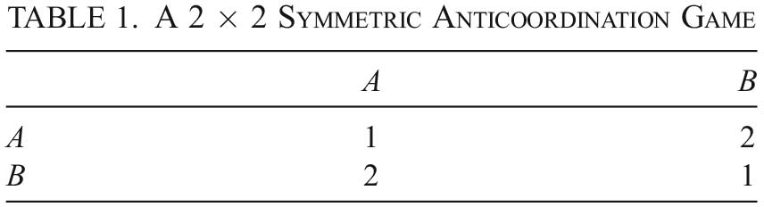
To understand our motivating puzzle, we can consider the simple anticoordination game given in table 1 and examine the predictions as to the evolutionary outcomes of its corresponding population game under each dynamics. For both dynamics, let us assume large populations, random pair-wise interactions, true breeding, the absence of mutation, and infinite-horizon play. Under the replicator dynamics, the prediction is that, from most all initial conditions, evolution will deliver the population to the polymorphic state $x=1/2$, where A-types and B-types coexist in equal proportions.Footnote ³ In contrast, for the same anticoordination game, the Moran process predicts that evolution will deliver the population, with equal probability, to one of the two monomorphic states $x=0$ or $x=1$, where the population is composed entirely of either A-types or B-types.Footnote ⁴ The evolutionary outcome that is a moral certainty in one model is an impossibility in the other.

Table 1.

A 2 × 2 Symmetric Anticoordination Game

Such a divergence in the predictions of the two dynamics leads naturally to the following questions: How are we deriving the predictions of each dynamics? And what is the cause of their divergence?Footnote ⁵

The standard explanation for divergence in such cases is that the dynamics differ in the time horizons of their predictions: the replicator dynamics approximates the short-to-medium-run behavior of evolution, while the Moran process can capture its long-run behavior (Taylor et al. Reference Taylor, Fudenberg, Sasaki and Nowak2004; Nowak Reference Nowak2006). The prediction of the replicator dynamics is polymorphism, and this is correct for the short-to-medium run. The prediction of the Moran process is monomorphism, and this is correct for the long run. Young (Reference Young1998, 47) states this clearly: “While [the replicator dynamics] may be a reasonable approximation of the short run (or even medium run) behavior of the process, however, it may be a very poor indicator of the long-run behavior of the process.”

The dynamics differ with respect to the time horizons of their predictions. This is true, but, in the case of interest, this is not the cause of the divergence in their predictions, and it is not the answer to our puzzle. The cause of the divergence lies in the standard technique employed to derive predictions from the Moran process, stochastic stability analysis, introduced to game theory by Foster and Young (Reference Foster and Young1990). Under conditions I will characterize, stochastic stability leads to the misprediction of homogeneity when long-run diversity is to be expected.

Why does this matter? In brief, because the technique of stochastic stability analysis is ubiquitous. Those having deployed stochastic stability in the analysis of the Moran process and related processes (e.g., the closely related Markov processes of Fermi and Wright-Fisher) include Young (Reference Young1993, Reference Young1998, Reference Young, Blume and Durlauf2006, Reference Young2015), Binmore, Samuelson, and Vaughan (Reference Binmore, Samuelson and Vaughan1995), Binmore and Samuelson (Reference Binmore and Samuelson1997), Fudenberg and Imhof (Reference Fudenberg and Imhof2004, Reference Fudenberg and Imhof2006), Nowak et al. (Reference Nowak, Sasaki, Taylor and Fudenberg2004), Taylor et al. (Reference Taylor, Fudenberg, Sasaki and Nowak2004), Fudenberg et al. (Reference Fudenberg, Nowak, Taylor and Imhof2006), Imhof and Nowak (Reference Imhof and Nowak2006), Nowak (Reference Nowak2006), Ohtsuki, Bordalo, and Nowak (Reference Ohtsuki, Bordalo and Nowak2007), Sandholm (Reference Sandholm2007, Reference Sandholm2009, Reference Sandholm2010, Reference Sandholm2012), and Traulsen and Hauert (Reference Traulsen, Hauert and Schuster2010). Evolutionary game theorists use stochastic stability analysis to explore and explain various phenomena in the domains of cultural and biological evolution, ranging from the diffusion of innovations to the emergence of conventions. Stochastic stability is a standard tool in both theoretical and applied work. Given this, understanding its limitations is important.

The structure of this article is as follows. In section 2, I introduce the replicator dynamics and Moran process models along with the concepts of asymptotic stability, replacement probabilities, and stochastic stability needed to understand our results. In section 3, I demonstrate the conditions under which stochastic stability will mispredict the long-run behavior of the Moran process, polymorphisms will persist, and the behavior of the replicator dynamics and Moran process will realign. In section 4, I discuss real-world applications in which one can expect my results will matter, and I suggest a methodological moral for evolutionary modeling. In section 5, I conclude.

2. The Dynamics

2.1. The Replicator Dynamics

The replicator dynamics is the “first and most important model of evolutionary game theory” (Cressman and Tao Reference Cressman and Tao2014, 10810). This is in part because it allows us to isolate the qualitative influence of selection on evolution, unperturbed by the complicating factors of mutation, drift, recombination, and so on. The leading idea behind the replicator dynamics is that types that are more fit than the population average grow in relative proportion, and types that are less fit than average shrink in proportion. This can be described by a system of differential equations:Footnote ⁶

${\dot{x}}_i=x_i\left[u\right(i,x)-u(x,x\left)\right]\text{\hspace{1em}for }i\in S,$

where S is the set of possible types, ${\dot{x}}_i$ denotes the rate of change of the population proportion of type i, x_i denotes the population proportion of type i, u(i, x) denotes the expected fitness for type i from interacting with the population, and u(x, x) denotes the population average fitness.

We derive predictions from the replicator dynamics by finding the asymptotically stable states of the dynamics for a given game and equating these with the plausible outcomes of evolution for that game.Footnote ⁷ A population state is asymptotically stable just in case it is both stable and attracting. Intuitively, a state is stable if states near it remain near it and attracting if states near it tend toward it. This gives us our prediction of the behavior of a process described by the replicator dynamics.

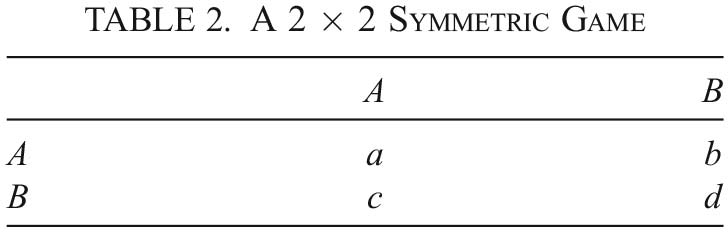
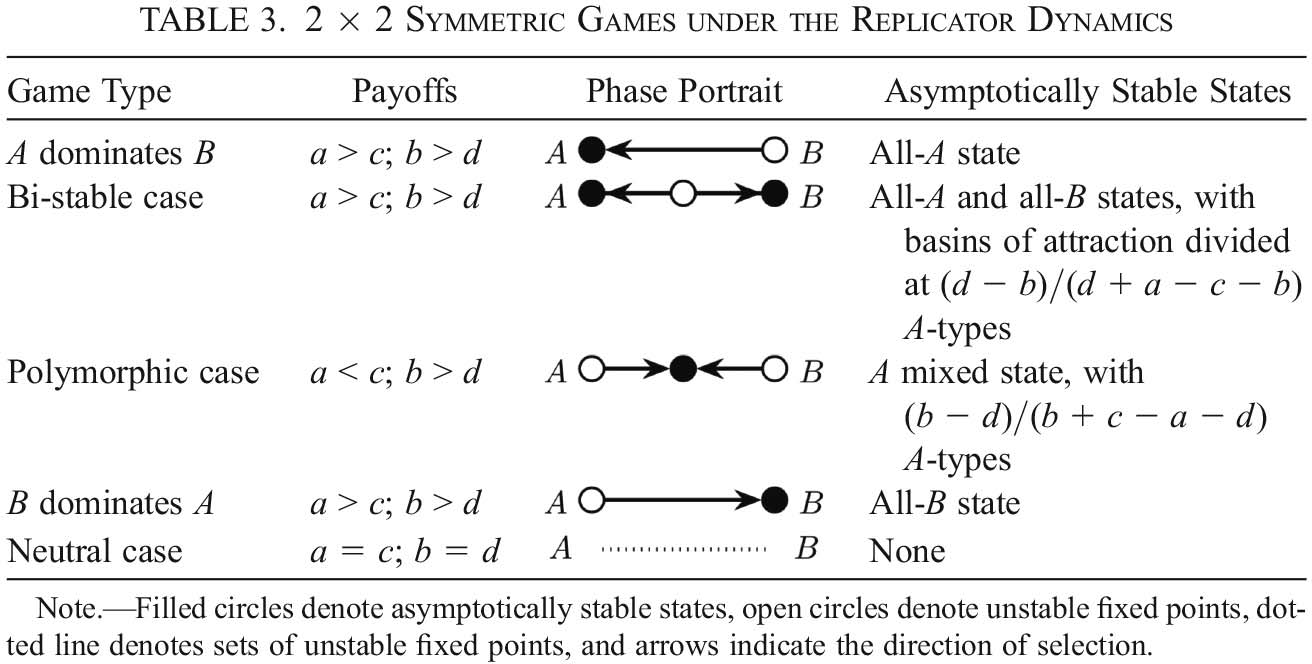
For the simple class of $2\times 2$ symmetric games (see table 2) under the replicator dynamics, five qualitatively distinct outcomes are possible. These can bee seen in table 3. Our puzzle concerns the class of anticoordination games, shown in the third row of the table and labeled the ‘polymorphic case’. This is where we find polymorphisms that are asymptotically stable under the replicator dynamics. Anticoordination games constitute an important class of interaction structures and have been used in explanations of ritualized animal conflict (Maynard Smith Reference Maynard Smith1974), sex ratios (Hamilton Reference Hamilton1967), and bargaining norms (Skyrms Reference Skyrms1996).

Table 2.

A 2 × 2 Symmetric Game

Table 3.

2 × 2 Symmetric Games under the Replicator Dynamics

Note. Filled circles denote asymptotically stable states, open circles denote unstable fixed points, dotted line denotes sets of unstable fixed points, and arrows indicate the direction of selection.

We derive the prediction of the replicator dynamics for anticoordination games (table 3, third row) as follows. We solve for the fixed points of the dynamics, where the rate of change in population proportions of each type is zero (i.e., ${\dot{x}}_1={\dot{x}}_2=0$). This yields three states: the two monomorphic states composed entirely of one type or the other and a polymorphic state (i.e., {0, $(b-d)/(b+c-a-d)$, 1}). We assess the stability of these states by examination of the eigenvalues of a Jacobian matrix for the dynamics, which reveals that only the mixed state is asymptotically stable. Given this, we know that a population starting at the polymorphism with proportion $(b-d)/(b+c-a-d)$ A-types will remain there and that, from most all initial conditions, the dynamics will converge to the polymorphism.Footnote ⁸

2.2. The Frequency-Dependent Moran Process

The Moran process is a birth-death process in which, for each time step, two individuals are chosen: one for reproduction and the other for elimination. The individual chosen for birth is determined, probabilistically, by the relative fitness of the types within the population, and the individual chosen for death is selected at random. So, if we consider a population of N individuals whose payoffs from interaction are described by table 2, then the fitnesses f_i , g_i of the types A, B can be described as functions of the number i of A-types,

$f_i=1-w+w\frac{a(i-1)+b(N-i)}{N-1}\text{\hspace{1em}and\hspace{1em}}{g}_i=1-w+w\frac{\mathrm{ci}+d(N-i-1)}{N-1}\text{,}$

where w denotes the intensity of selection, or the game’s contribution to the net fitness of the organism. Observe that $w=1$ implies that an individual’s fitness is entirely determined by her interactions in this game, and $w=0$ implies that the game makes no contribution to her fitness.

Individuals reproduce at a rate proportional to their fitness. The rate of reproduction then for A -types is if_i and for B-types is $(N-i)g_i$. Each period, one offspring is chosen at random to enter the population. So, the probability of adding an A-type offspring is ${\mathrm{if}}_i/[{\mathrm{if}}_i+(N-i\left)g_i\right]$, and the probability of adding a B-type offspring is $(N-i)g_i/[{\mathrm{if}}_i+(N-i\left)g_i\right]$. After reproduction, one individual is chosen at random to be removed from the population, so that with probability $i/N$ an A-type is removed, and with probability $(N-i)/N$ a B-type is removed. This makes it so that the population size remains constant.

Formally, we define the Moran process with population size N as a Markov process {$X_t^N$} over the finite state space $\chi =\{1,\dots ,N\}$ of possible population states, with transition probabilities between states given by

$P_{i,j}=\{\begin{array}{cc}\frac{N-i}{N}\frac{{\mathrm{if}}_i}{{\mathrm{if}}_i+(N-i)g_i},& \text{if }j=i+1\\ \frac{i}{N}\frac{(N-i)g_i}{{\mathrm{if}}_i+(N-i)g_i},& \text{if }j=i-1\\ 1-P_{i,i+1}-P_{i,i-1},& \text{if }j=i\\ 0,& \text{otherwise,}\end{array}$

which composes a tridiagonal matrix. Note that $P_{0,0}=P_{N,N}=1$, so that the process has two absorbing states, $i=0$ and $i=N$, and that all other states are transient. An absorbing state is a state that, once visited by the process, is never escaped. A transient state then is one that will only be visited a finite number of times before the process arrives at some absorbing state. Note that, in the limit of time, with probability 1, the process will reach one or the other absorbing state.

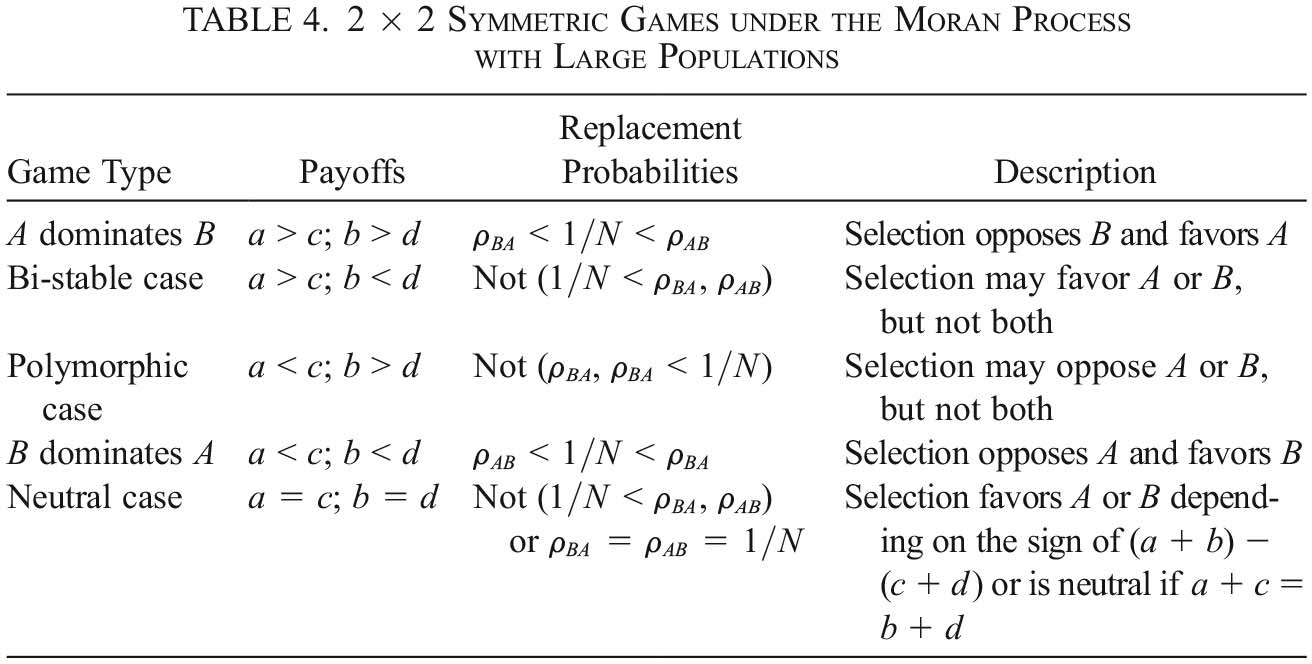
For the simple class of $2\times 2$ symmetric games under the Moran process, as with the replicator dynamics, we can examine five distinct cases (table 4) when the population size is large.Footnote ⁹ For each case, the outcomes are described in terms of the relative probability of arrival of the process at each of the absorbing states. In particular, we compare the probability of a single mutant coming to replace the incumbent type and take over the population. This yields the replacement probabilities ρ _AB and ρ _BA , where ρ _AB denotes the probability of a single A-type individual leading to the takeover of an otherwise B-type population, and ρ _BA denotes the probabilities of the inverse process.Footnote ¹⁰ The replacement probabilities of types are compared to those of a neutral mutant (where $a=b=c=d$), which will come to fixation with probability $1/N$. We say that selection favors a type if its replacement probability is greater than that of a neutral mutant and that selection opposes a type if its replacement probability is less than that of a neutral mutant.

Table 4.

2 × 2 Symmetric Games under the Moran Process with Large Populations

We derive the predictions of the Moran process for anticoordination games (table 4, third row) by calculating the replacement probabilities for each type. This yields three possibilities: ${\rho }_{\mathrm{BA}}<1/N<{\rho }_{\mathrm{AB}}$, ${\rho }_{\mathrm{AB}}<1/N<{\rho }_{\mathrm{BA}}$, or $1/N<{\rho }_{\mathrm{AB}}$, ρ _BA . That is, either selection favors one type replacing the other, or it favors both replacing one another.Footnote ¹¹ What we see is that, for anticoordination games, selection must favor at least one type in coming to dominate the population. In the absence of mutation, polymorphism is temporary, and the population inevitably attains homogeneity.

2.3. The Frequency-Dependent Moran Process with Mutation

With the introduction of mutation, the behavior of the Moran process changes qualitatively. Absorbing states disappear, and there is positive probability that the process will transit within a finite time from any given state to any other. Thus, in the limit of time, the process visits each state infinitely often. Since absorption will not occur, replacement probabilities are no longer appropriate, and a different method of analyzing the behavior of the process is needed. This method is to find the long-run distribution of time spent by the process over the possible population states.

Formally, we define the Moran process with population size N and mutation rate η as an ergodic process {$X_t^{N,\eta }$} over the finite state space $\chi =\{1,\dots ,N\}$, with transition probabilities given by

${\hat{P}}_{i,j}=\{\begin{array}{cc}(1-\eta )\frac{N-i}{N}\frac{{\mathrm{if}}_i}{{\mathrm{if}}_i+(N-i)g_i}+\eta \frac{N-i}{N}\frac{(N-i)g_i}{{\mathrm{if}}_i+(N-i)g_i},& \text{if }j=i+1\\ (1-\eta )\frac{i}{N}\frac{(N-i)g_i}{{\mathrm{if}}_i+(N-i)g_i}+\eta \frac{i}{N}\frac{{\mathrm{if}}_i}{{\mathrm{if}}_i+(N-i)g_i},& \text{if }j=i-1\\ 1-{\hat{P}}_{i,i+1}-{\hat{P}}_{i,i-1},& \text{if }j=i\\ 0,& \text{otherwise},\end{array}$

where ${\hat{P}}_{0,0}={\hat{P}}_{N,N}=1-\eta$.Footnote ¹² Note the mutation terms. What they capture is that, most of the time ($1-\eta$), selection behaves as normal, but in a minority of instances η, an offspring that was to be an A-type will become a B-type and vice versa.Footnote ¹³

Now, to understand the long-term behavior of the Moran process, we can compute its stationary distribution that captures the proportion of time spent at each population state. Formally, a probability distribution $\mu \in {ℝ}^{\chi }$ is a stationary distribution of the ergodic process {$X_t^{N,\eta }$} if

$\sum _{i\in \chi }{\mu }_i{P}_{i,j}=\mu ,\text{\hspace{1em}for all }j\in \chi \text{.}$

That is, a stationary distribution is a probability vector such that taking its product with the matrix of transition probabilities simply returns itself.

We know that such a distribution exists, since every ergodic process has a unique stationary distribution, and that it is history independent. That is, from any initial distribution over states, the distribution of time spent by the process over population states converges to that given by stationary distribution.

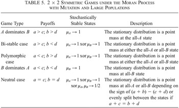
Typically, however, we do not derive predictions from the Moran process by finding its stationary distribution. This is because general analytic forms of the stationary distribution for the Moran process for complex games are not known and because the stationary distribution applies positive probability to every state, as opposed to yielding unique predictions (Harper and Fryer Reference Harper and Fryer2016).Footnote ¹⁴

Instead, the desire for analytic tractability and unique equilibrium prediction motivates the use of an alternative method: stochastically stability analysis. Stochastically stable states are just those that retain mass in the stationary distribution when we take the limit as mutation approaches 0.Footnote ¹⁵ Formally, a state $i\in \chi$ is stochastically stable if

$\underset{\eta \to 0}{\lim }{\mu }_i^{N,\eta }>0.$

We saw that, for the Moran process, in the absence of mutation, all and only monomorphic states were absorbing states. Now, with vanishing mutation, the stationary distribution collapses (typically) to a point mass on just one of these absorbing states. As mutation vanishes, the behavior of the ergodic process approaches that of the absorbing chain and so spends most of its time near one or another monomorphic state.

We derive the predictions of the Moran process with mutation for anticoordination games (table 5, third row) by finding that states retain positive mass in stationary distribution as mutation vanishes.Footnote ¹⁶ This yields two possibilities: ${\mu }_A\to 1$ or ${\mu }_B\to 1$.Footnote ¹⁷ That is, either the all-A or all-B state, but not both, can be stochastically stable. Once again, polymorphism cannot be selected.

Table 5.

2 × 2 Symmetric Games under the Moran Process with Mutation and Large Populations

3. The Long-Run Persistence of Diversity

Why can stochastically stable states not be polymorphisms? This is by construction: a stochastically stable state of an ergodic process will be an absorbing state of its corresponding absorbing chain. Stochastic stability is defined for an ergodic process and is determined by identifying the states that retain mass in the stationary distribution of the process as mutation vanishes. As mutation vanishes, the behavior of the ergodic process approaches that of the absorbing chain. Polymorphisms cannot be absorbing states and, thus, cannot be stochastically stable.

In most of the game types, the qualitative predictions of asymptotic stability for the replicator dynamics and the predictions of stochastic stability for the Moran process are in basic agreement (see tables 3–5). That is, in coordination games and dominating strategy games (rows 1, 2, 4), for large populations, the asymptotically stable state with the largest basin of attraction has the greatest replacement probability and is uniquely stochastically stable. Predictions differ in the polymorphic case (compare row 3 of tables 3–5) and the neutral case (compare row 5 of tables 3–5). The latter is to be expected, as the replicator dynamics explicitly abstracts away from the effects of drift. Disagreement about the polymorphic case is more puzzling. For an anticoordination game, polymorphism is uniquely asymptotically stable under the replicator dynamics, but only monomorphic states can be stochastically stable under the Moran process.

The standard explanation we have seen accounts for this divergence in predictions, by positing that the replicator dynamics fails to capture the long-run behavior of the Moran process. The Moran process will, due to stochasticity, eventually arrive at an absorbing state of the process, where it will spend most of its time, trapped by low mutation rates. The following excerpt from Sandholm (Reference Sandholm2009, 208) tells this story:

Young (Reference Young1998, 20) calls this the “punctuated equilibrium effect,” echoing that “when the stochastic shocks are small, the mode of this frequency distribution [the stationary distribution] will tend to be close to the stochastically stable [states] predicted by the theory.”

But this characterization turns out to be insufficient for the polymorphic case. How small must the mutation rate be? And what role do population size and intensity of selection play? In anticoordination games under the Moran process, the population may indeed spend the majority of its time at or near a polymorphic equilibrium, even in the long run. This occurs when there is small but nonvanishing mutation and sufficiently large population size and intensity of selection.

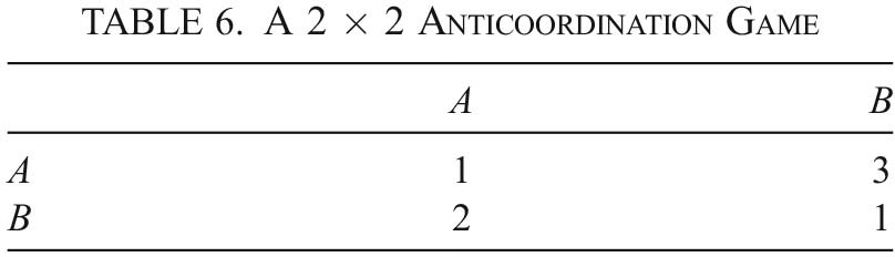
To illustrate the potential divergence of the actual and predicted behaviors of the Moran process, consider the anticoordination game given by table 6. We fix the following parameter settings: population size $N=100$, mutation rate $\eta =0.01$, and intensity of selection $w=0.2$. Now, consider the predictions of each of our stability concepts: the replacement probabilities are ${\rho }_{\mathrm{AB}}\approx 0.1644$ and ${\rho }_{\mathrm{BA}}\approx 0$, so selection favors A and opposes B; absorption into the all-A state is the most probable outcome of the process. Stochastic stability analysis yields that ${\mu }_A=1$, so all-A is the unique stochastically stable state; in the long run, the process will spend almost all of its time near the all-A state. Finally, asymptotic stability analysis yields the unique asymptotically stable state $x^{*}=2/3$; from all mixed initial conditions the population will converge to a polymorphism where $2/3$ of the population are A-types and $1/3$ are B-types.

Table 6.

A 2 × 2 Anticoordination Game

	A	B
A	1	3
B	2	1

To see whether these predictions hold up, I analytically derive the actual long-run behavior of the Moran process by calculating its stationary distribution, without vanishing mutation, but rather with fixed parameter values of mutation rate.Footnote ¹⁸ This stationary distribution is plotted in figure 1. Notice that the mode of the stationary distribution is at the state where there are 67 A-types in the 100-individual population. The process spends the most time precisely at the polymorphic state predicted by asymptotic stability under the replicator dynamics, not at the all-A state that is stochastically stable.

Figure 1.

Stationary distribution for the Moran process with population size $N=100$, mutation rate $\eta =0.01$, and intensity of selection $w=0.2$. Vertical line marks the mode of the distribution.

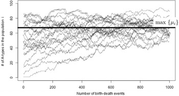
To get a feel for the medium-run behavior of the Moran process, we can simulate several dozen individual population trajectories, starting from random initial conditions and evolving over a thousand birth-death events. This is plotted in figure 2. Again, it is clear that asymptotic stability under the replicator dynamics gives us a more accurate prediction of the behavior of the Moran process.

Figure 2.

Plot of 35 population trajectories for the Moran process over 1,000 birth-death events. Horizontal bar corresponds to the peak of the stationary distribution.

What we see is stochastic stability mispredicting the actual behavior of the Moran process under particular conditions. But we want a more general characterization of when this will occur. To obtain this, we turn first to the case in which there is no selection $w=0$. Here, I use the detailed balance conditions of ergodic processes (Karlin and Taylor Reference Karlin and Taylor2012) to deduce when the mass of the stationary distribution will be increasing toward the center of the state space, that is, the conditions under which the peak of the stationary distribution will be at a polymorphic state. This is captured by the following lemma.

What I am calling the ‘strong mutation condition’ corresponds to when the expected number of mutants entering a population in $N+2$ birth-death events is greater than 1. Intuitively, here strong mutation gives us when either the population is sufficiently large such that the process rarely arrives at monomorphic states or the mutation rate is sufficiently high such that, when the population does arrive at monomorphic states, it does not spend too much time there.

Note that strong mutation is both necessary and sufficient for the stationary distribution to exhibit a polymorphic peak (fig. 3). That is, just when $\eta (N+2)>1$, the stationary distribution is concave and climbs gradually toward its peak near the middle point $(N+1)/2$ from either side of the state space (fig. 3a ). When $\eta (N+2)=1$, the stationary distribution is uniform (fig. 3b ). When $\eta (N+2)<1$, the stationary distribution is convex and climbs outward from its nadir near the middle point toward its peaks at the monomorphic states 0 and N (fig. 3c ).

Figure 3.

In the absence of selection pressures $w=0$, satisfaction of the strong mutation condition $\eta \left(N+1\right)>1$ determines the shape of the stationary distribution. a, $\eta \left(N+2\right)>1$; b, $\eta \left(N+2\right)=1$; c, $\eta \left(N+2\right)<1$.

We can use this insight as we turn to consider the case of nonzero intensity of selection $w>0$. Consider the dynamics of an anticoordination game characterized by the payoffs $a<c$ and $b>d$. It may be intuitive that, when the stationary distribution is already increasing in mass toward a polymorphic state, the addition of selection pressure toward an interior equilibrium will continue to produce an interior mode. This is the essential insight from which I will derive my main result.

Before doing so, however, there are two stipulations that need to be made. First, I follow Taylor et al. (Reference Taylor, Fudenberg, Sasaki and Nowak2004) in requiring that a coordination game, characterized by $a<c$ and $b>d$, further satisfy the condition that $b-d>(a-d)/N>a-c$ for finite populations. This is because, for finite populations, the qualitative dynamics of a game can be affected by the anticorrelation produced by individuals not interacting with themselves. Anticorrelation can alter the qualitative dynamics of the game. Indeed, in sufficiently small populations, each of our four game types can, in principle, be transformed into a different game.

To see why this is so, consider the case with a population composed of two individuals $N=2$. Here, the process has three possible population states: two A-types, two B-types, and one of each type. Since transition out of each monomorphic state occurs solely via mutation, only the state in which there is one of each type involves selection. In this state, only the difference of the values in the off-diagonal of the payoff matrix, $b-c$, matters. If $b-c>0$, then A dominates B. If $b-c<0$, then B dominates A. The game is no longer, qualitatively, an anticoordination game.

To correct for this, we require that payoffs further satisfy $b-d>(a-d)/N>a-c$, ensuring that the game retains the qualitative dynamics of anticoordination.Footnote ¹⁹ When N grows large, this condition is easily satisfied, and the qualitative dynamics are once again determined by the signs of the differences of the values of the column vectors, $a-c$ and $b-d$, just as with the replicator dynamics.

Second, I must also stipulate that mutation rates be reasonable: $\eta <1/2$. It should be clear why this is so. If it is more probable that birth events are produced by mutation than by selection, then the fitnesses of the types will be reversed, and we will once again be playing a different game—a coordination game, in fact.

With these two stipulations in hand, we can turn to a sufficient condition for the persistence of diversity of types under the Moran process.

What we have is that, when the strong mutation condition is satisfied, the peak of the stationary distribution is guaranteed to be between the midpoint of the state space and a critical point $i^{*}=\left[N\right(b-d)+d-a]/(b+c-a-d)$ that rapidly approaches the asymptotically stable state of the same game under the replicator dynamics $x^{*}=(b-d)/(b+c-a-d)$ as N grows large.Footnote ²⁰

What remains is for us to confirm that, as intensity of selection increases, the peak of the stationary distribution will move toward the critical point. We can answer this in the affirmative.

This is good. I note, however, that strong mutation provides sufficient, and not necessary, conditions for a polymorphic mode of the stationary distribution. An anticoordination game can fail to satisfy the strong mutation condition but have it so that a peak of its stationary distribution is at a polymorphic state. Strong mutation ensures that the stationary distribution increases monotonically toward some interior equilibrium and, thus, ensures that there are no other peaks at the monomorphic states. For anticoordination games in which $\eta (N+2)$ is slightly less than 1 but selection pressure is great with $a\ll c$ or $b\gg d$, the highest peak of the stationary distribution may still be a polymorphic state, with other smaller peaks at the monomorphic states.

In sum, when strong mutation obtains for an anticoordination game, we know—with certainty—that stochastic stability analysis will mispredict a monomorphic outcome when polymorphism is to be expected. But, when strong mutation does not obtain, there is still the possibility of misprediction.

To get an idea of the conditions under which games will exhibit polymorphic modes near the replicator dynamics prediction, we can examine the peak of the stationary distribution of a representative anticoordination game (table 6) for different values of N, η, and w.

In figure 4, the darkness of each point in a plot encodes the distance, in terms of population proportion, between the peak of the stationary distribution and the replicator dynamics prediction. In the plots, population sizes $N\in \{2,3,\dots ,100\}$ vary along the x-axes, mutation rates $\eta \in \{0,0.01,\dots ,0.5\}$ vary along the y-axes, and intensities of selection $w\in \{{10}^{\mathrm{-2}},{10}^{\mathrm{-1}},1\}$ vary between plots.

Figure 4.

Distances of the mode of the stationary distribution from the replicator dynamics prediction for different values of N, η, w. Curve corresponds to $\eta (N+2)=1$, above which the strong mutation condition is satisfied. a, $w={10}^{\mathrm{-2}}$; b, $w={10}^{\mathrm{-1}}$; c, $w=1$.

This accords with what we have learned so far and illustrates our results. Where strong mutation obtains (in the space above the curves), the peak of the stationary distribution is near the replicator dynamics prediction x*. When the intensity of selection is low, $w={10}^{\mathrm{-2}}$, the demarcation is quite precise. As intensity of selection increases, $w={10}^{\mathrm{-1}}$, a growing range of population sizes and mutation rates (just beneath the curve) will be compatible with an interior mode near x*. When intensity of selection is at its maximum, $w=1$, strong mutation will continue to provide a sufficient, but not necessary, condition for polymorphism.

4. Discussion

I have characterized conditions under which we can anticipate that the behavior of the Moran process will be mischaracterized by stochastic stability and when long-term diversity will persist. But should we expect these conditions to obtain in nature? If, indeed, the strong mutation condition were never to be satisfied, then we might comfortably rely on stochastic stability analysis without fear of it leading us astray. To see whether this is so, we can survey representative population sizes, mutation rates, and intensities of selection from relevant real-world evolving populations.

Considering the canonical case of E. coli bacteria, we have that the per-site mutation rates are typically of the order of 10⁻⁴ mutations per allele per replication (Tenaillon et al. Reference Tenaillon, Barrick, Ribeck, Deatherage, Blanchard, Dasgupta, Wu, Wielgoss, Cruveiller, Médigue, Schneider and Lenski2016). That is, an expected 1 out of 5,000 bacteria produced carry at least one mutation at a locus of interest. Typical bacterial populations, however, are of the order of 10⁶–10⁸. This yields a mutation strength of $\eta (N+2)\approx \mathrm{20,000}$. That is, there will be an average of 20,000 mutations per population per generation. This is deep into the territory of strong mutation. Moreover, the population sizes and mutations rates of many bacteria are comparable (Drake et al. Reference Drake, Charlesworth, Charlesworth and Crow1998). Bacterial populations, it seems, will exhibit population sizes and mutation rates that suggest their long-run evolutionary behavior will typically be at odds with the predictions of stochastic stability.

Humans, however, exhibit per-allele mutation rates ranging from 10⁻⁵ to 10⁻¹⁰ (Drake et al. Reference Drake, Charlesworth, Charlesworth and Crow1998). Throughout much of our evolutionary history, H. sapiens subsisted in hunter-gatherer groups averaging 50–150 individuals (Bowles and Gintis Reference Bowles and Gintis2011). Hence, human biological evolution will typically not satisfy strong mutation. The same will be true of many complex organisms, such as mammals (Kumar and Subramanian Reference Kumar and Subramanian2002).

However, in the case of cultural evolution, we expect mutation rates—or noise in the transmission of behavior via social learning and imitation—to be potentially much higher (Boyd and Richerson Reference Boyd and Richerson1985). Taking the example of humans, for a group of 100 individuals, an innovation or error rate in behavior transmission of just over 10% would satisfy strong mutation. Given that the Moran process is often used to model processes of cultural evolution, it will be important to know when an evolutionary process satisfies the strong mutation condition.

We should note that the relationship between strong mutation and persistent polymorphism is not guaranteed to hold in other game structures. We can expect the analysis will vary for extensive-form games, with more players and strategies, and with the introduction of social or spatial structure, and so on. But it is reasonable to imagine that qualitatively similar conditions may hold for other classes of games. The question as to the limits of the agreement of the dynamics for the case of strong mutation provides an interesting topic for further study.

5. Conclusion

The puzzle of the divergence between the predictions of the replicator dynamics and the Moran process finds its resolution in identifying a shortcoming of stochastic stability analysis. The cause of misprediction by stochastic stability is the assumption of vanishing mutation. Polymorphism, which cannot be stochastically stable, can still be the most probable long-run outcome of the Moran process.

I have shown that, under a range of values of population size, mutation rate, and intensity of selection, the Moran process leads to polymorphisms that characterize the long-run behavior of the process. My results show that anticoordination games, and games containing anticoordination subgames, can exhibit this behavior for a broad range of conditions. For the $2\times 2$ anticoordination games considered here, ‘strong mutation’ provides a sufficient condition for misprediction by stochastic stability analysis of the long-run behavior of the Moran process. Moreover, in the presence of strong mutation, the Moran process will typically spend most of its time near the specific polymorphic state that is asymptotically stable under replicator dynamics.

We have also seen that strong mutation will be satisfied by a range of real-world evolutionary processes. This is particularly true when population sizes are large, such as with bacterial colonies, and when mutation or noise rates are high, as is typical in the transmission of behavior in models of cultural evolution. In such cases, we can anticipate that the behavior of the Moran process will be mischaracterized by stochastic stability and will realign with the predictions of the replicator dynamics.

The upshots of our analysis are that we can characterize the conditions under which an evolutionary process described by the Moran process (1) will sustain long-run diversity, (2) realign with the predictions of the replicator dynamics, and (3) should not be analyzed using stochastic stability. Our moral is that, when we anticipate attracting polymorphic equilibriums—that is, when a population interaction structure is characterized by anticoordination—stochastic stability may be an unreliable predictor of even the long-term behavior of evolution. In such cases, analysis should proceed by computing the stationary distribution explicitly using representative values of population size, mutation rate, and intensity of selection. When such an approach is not feasible, simulation methods may suffice. In normal science, we can keep our best analytic tools, shortcomings and all, but we must also learn when not to employ them.