





1. Introduction
Patagonia is a hotspot of ice loss in the Andes, accounting for over 80% of regional glacier mass loss (Braun and others, Reference Braun2019; Dussaillant and others, Reference Dussaillant2019). This loss is concentrated in the Southern (SPI) and Northern Patagonian Icefields (NPI), dominated by large calving outlet glaciers (Minowa and others, Reference Minowa, Schaefer, Sugiyama, Sakakibara and Skvarca2021). In these glaciers, frontal ablation encompassing iceberg calving and subaqueous melt drives highly nonlinear glacier responses to climatic forcing and can partially decouple ice dynamics from climate (e.g. Pfeffer, Reference Pfeffer2007; Choi and others, Reference Choi, Morlighem, Wood and Bondzio2018). Outside these icefields, frontal ablation remains unexplored.
Northern Patagonia (35°–45° S) is characterized by warmer and less humid conditions, with winter-dominated precipitation (PP), unlike the year-round PP in Southern Patagonian Andes (45°–53° S) (Garreaud and others, Reference Garreaud, Lopez, Minvielle and Rojas2013). Glaciers in Northern Patagonia develop smaller and shallower proglacial lakes, which are often unstable and prone to sudden drainage events known as glacial lake outburst floods (GLOFs) (Carrivick and Tweed, Reference Carrivick and Tweed2016). The area of these lakes increased by ∼50% between 1986 and 2016 (Wilson and others, Reference Wilson2018). In this region, frontal ablation may be more strongly modulated by local factors such as valley geometry (e.g. Watson and others, Reference Watson, Kargel, Shugar, Haritashya, Schiassi and Furfaro2020), seasonal ice cover and transient hydrological and thermal perturbations (Mallalieu and others, Reference Mallalieu, Carrivick, Quincey and Smith2020), requiring high-resolution observations to quantify.
The fluxgate method is the standard approach to estimate frontal ablation. It calculates ice discharge through a cross-section located upstream from the glacier front to avoid regions already replaced by water (e.g. McNabb and others, Reference McNabb, Hock and Huss2015; Minowa and others, Reference Minowa, Schaefer, Sugiyama, Sakakibara and Skvarca2021; Kochtitzky and others, Reference Kochtitzky2022; Caldwell and others, Reference Caldwell2025). While this approach accounts for spatial variations in ice thickness and surface velocity across the fluxgate, the cross-section may be located hundreds of meters to several kilometers upstream from the terminus. Thus, it does not fully capture spatial variability in velocity and thickness along the calving front itself. It also requires correcting for surface mass balance (SMB) over the down-glacier area, adding a potential source of uncertainty.
Here, we build on the approach of Johnson and Floricioiu (Reference Johnson and Floricioiu2019) and Johnson and others (Reference Johnson, Han, Floricioiu and Bässler2016) to estimate frontal ablation using a multiple fluxgate method. Subdividing the terminus into several fluxgates captures the coexistence of advances, stagnation and retreats along the ice front. By computing frontal ablation close to the calving front, the contribution of SMB is reduced and remains within the method’s uncertainty.
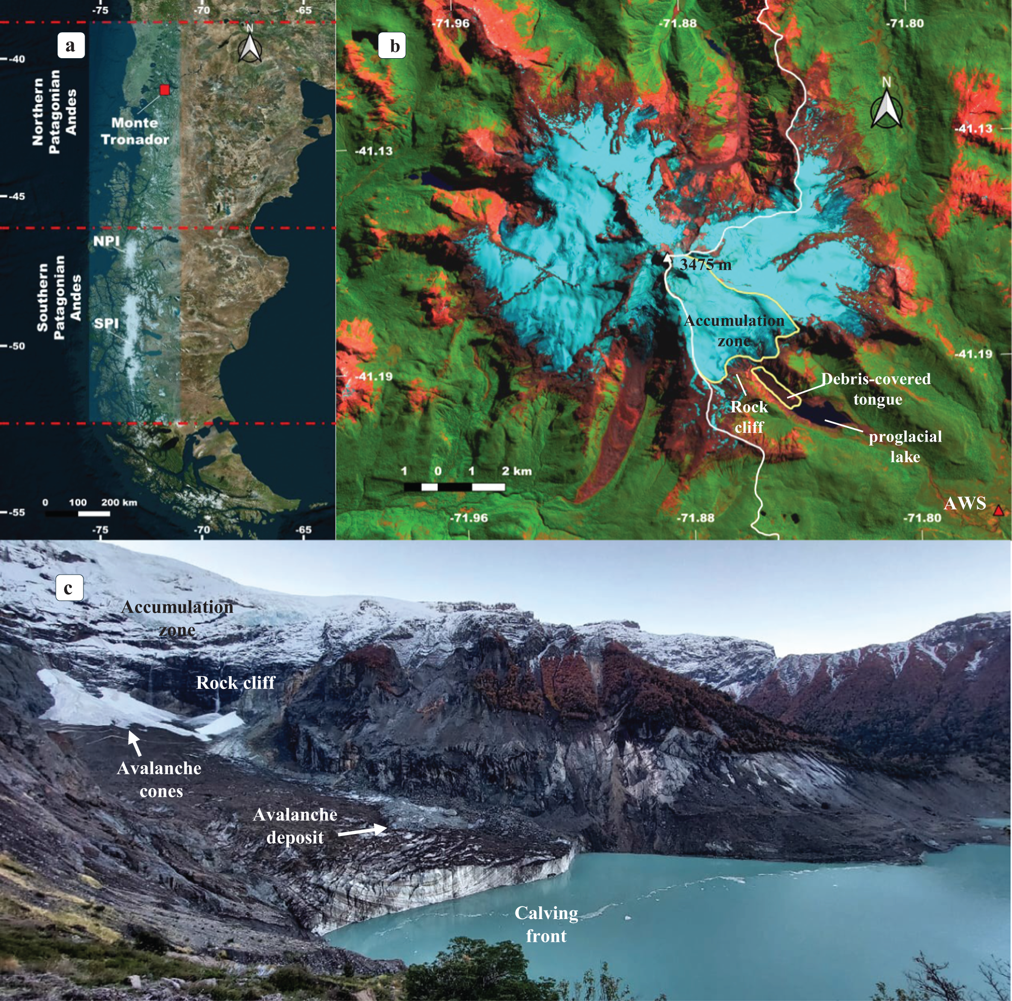
We present a novel application of this framework to Manso Glacier in Monte Tronador, Northern Patagonia (Fig. 1a), estimating frontal ablation at subseasonal (40–90 days) and annual scales for 2017–24 and 2013–23, respectively. We then assess the relationship between frontal ablation rate and environmental variables. This work provides the first estimate of frontal ablation in Patagonia outside the two main icefields.
(a) Monte Tronador and Patagonian Icefields location (background: ESRI Terrain image). (b) Sentinel-2 false color image from 29 February 2024 of Monte Tronador (SWIR-NIR-red bands). Manso Glacier is outlined in pale yellow, and the international limit in white. (c) Photo of Manso Glacier tongue from the southern margin, April 2024.

Figure 1 Long description
A) Map showing Monte Tronador's location in Northern Patagonia Andes, with NPI and SPI marked. The map includes latitude and longitude lines, with Monte Tronador highlighted. B) Sentinel-2 false color image of Monte Tronador, displaying SWIR-NIR-red bands. Features include the accumulation zone, rock cliff, debris-covered tongue, and proglacial lake. The international limit is outlined in white, and Manso Glacier is marked in pale yellow. Coordinates and elevation of 3475 meters are noted. C) Photo of Manso Glacier's southern margin, showing the accumulation zone, rock cliff, avalanche cones, avalanche deposit, and calving front. The glacier is adjacent to a lake, with visible snow and ice formations.
2. Study area: Manso Glacier
Manso Glacier (9.1 km2 in 2022) is the largest and the only calving glacier of Monte Tronador (3475 m.a.s.l.; 41.15° S, 71.88° W), an extinct Pleistocene stratovolcano straddling the Argentina–Chile border (Fig. 1b). This valley glacier is one of the most iconic tourist attractions of Nahuel Huapi National Park. The accumulation zone is located between 3100 and 2000 m and ends in a ∼400 m-high cliff between 1900 and 1500 m. Below the cliff, the ablation zone forms a regenerated debris-covered tongue, 1.7 km long and 400 m wide in 2023, nourished by frequent avalanches (Fig. 1c). Ice thickness at the tongue can reach 240 m (Zorzut and others, Reference Zorzut, Ruiz, Rivera, Pitte, Villalba and Medrzycka2020).
The glacier has shown a delayed response to the trend of warming air temperature ( $T_{air}^\circ $) and decreasing PP in Northern Patagonia (Bown and Rivera, Reference Bown and Rivera2007; Masiokas and others, Reference Masiokas, Luckman, Villalba, Ripalta and Rabassa2010), with the ice front in contact with Little Ice Age moraines until 2000, when the proglacial lake started to grow rapidly.
Manso proglacial lake shows the largest proglacial lake expansion recorded in the Southern Andes between 2000 and 2016 (Wilson and others, Reference Wilson2018). The lake expanded from 0.18 km2 in 2000 to 0.66 km2 in 2009 (∼0.05 km2 a−1), after which growth slowed, reaching 0.93 km2 by 2024 (∼0.02 km2 a−1).
In 2009, continued glacier retreat and lake growth triggered a GLOF due to the failure of an ice-cored moraine, amplified by intense rainfall (Worni and others, Reference Worni, Stoffel, Huggel, Volz, Casteller and Luckman2012). After the GLOF, the glacier terminus collapsed, and the lake resumed its expansion. The modern lake volume is twice the pre-GLOF volume, posing a significant risk to residents.
3. Data and methods
Our method computes frontal ablation as an ice volume and requires data of surface velocity, glacier extent, initial ice thickness, thickness change rates and flowlines as input. We first describe these datasets and then present the method, its uncertainty analysis and parameter settings. Finally, we introduce the additional datasets and methods used for the complementary analyses performed in this study.
3.1. Input data
3.1.1. Velocity
We derived surface velocity and flow direction grids using the Glacier Image Velocimeter (GIV) feature-tracking algorithm (Van Wyk De Vries and Wickert, Reference Van Wyk De Vries and Wickert2021) applied to Landsat-7 and Landsat-8 Top of Atmosphere (TOA) and Sentinel-2 L1C images (Table 1). Previous applications of GIV have relied exclusively on Sentinel-2 imagery (e.g. Van Wyk De Vries and others, Reference Van Wyk De Vries, Carchipulla-Morales, Wickert and Minaya2022; Troilo and others, Reference Troilo, Dematteis, Zucca, Funk and Giordan2024).
Optical imagery input for the GIV feature tracking algorithm.

Table 1 Long description
The table content is not included, so the subject measured and the row and column labels cannot be identified. No numeric values, categories, units, or time periods are available to read out. Because the cells are missing, no key data points, comparisons, or trends can be described.
The GIV algorithm yields monthly velocities and summary statistics (mean and median velocities) computed from all input images in the folder. Each folder spans a full hydrologic year (1 April–31 March in the Southern Hemisphere), so the resulting averages correspond to annual velocities.
Post-processing of velocity grids included resampling, directional filtering, interpolation and smoothing. The aspect grid (original pixel size 4 m) derived from the 2012 Pléiades digital elevation model (DEM; Ruiz and others, Reference Ruiz, Berthier, Viale, Pitte and Masiokas2017) was resampled to the velocity grid resolution (four times coarser than the input optical imagery) to reduce the influence of small-scale surface roughness and DEM noise and combined with the velocity fields. Pixels where flow direction deviated by more than 60° from terrain aspect were removed from both the flow direction and surface velocity grids (Ruiz and others, Reference Ruiz, Berthier, Masiokas, Pitte and Villalba2015). Remaining gaps within the glacier extent were filled using spline interpolation, and a 3 × 3 low-pass filter was applied to obtain smooth surface velocity fields.
Since 2013, surface velocity at the Manso Glacier tongue has been monitored twice a year using two ablation stakes surveyed with static Global Navigation Satellite System (GNSS) measurements, providing high-accuracy point velocities and SMB data. Feature-tracking parameters (signal-to-noise ratio [SNR], peak ratio and filters) were calibrated by comparing surface velocity magnitude and flow direction with GNSS observations. As velocity maps are scarce in winter due to limited optical imagery, validation relied on independent summer GNSS measurements. Comparisons with monthly feature-tracking velocity grids show small biases (−0.005 to −0.034 m d−1), low dispersion (SD 0.023–0.050 m d−1) and relative errors below ∼10%, relative to typical stake velocities of ∼0.4 m d−1, averaged over consecutive measurements per stake (Supplementary Fig. S1).
3.1.2. Ice thickness
We used the ice thickness modeled for 2012 from Zorzut and others (Reference Zorzut, Ruiz, Rivera, Pitte, Villalba and Medrzycka2020) as the initial thickness. This thickness was derived through an inversion based on the parallel flow approximation, combining surface velocity and elevation data from high-resolution Pléiades imagery with ground-penetrating radar (GPR) measurements. The GPR dataset comprises 23.8 km of airborne surveys across nine glaciers of Monte Tronador and 3.2 km of ground-based surveys over the debris-covered tongue of Manso Glacier (Supplementary Fig. S2a), with uncertainties of ±4 and ±17 m, respectively, based on vertical resolution (half the radar wavelength). These data were used to calibrate and validate the model, which has a spatial resolution of 16 m and yields a root-mean-square error (RMSE) of ∼31 m for the optimal smoothing scale.
3.1.3. Thickness change rate
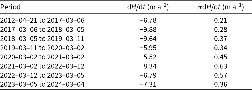
A first Pléiades acquisition of Manso Glacier was made on 21 April 2012, and since March 2017, stereoscopic pairs have been acquired each year at the end of summer (March). The stereoscopic images were processed using the Ames Stereo Pipeline photogrammetry software (Beyer and others, Reference Beyer, Alexandrov and McMichael2018), using the semi-global matching algorithm and the parameter set from Deschamps-Berger and others (Reference Deschamps-Berger2020) to generate DEMs with a ground sampling distance of 4 m. The 21 April 2012 DEM was then chosen as the reference DEM. All other DEMs were co-registered to this reference following Nuth and Kääb (Reference Nuth and Kääb2011), after excluding glaciers and slopes greater than 40°. In addition, a bias correction was applied to account for any tilt and mitigate the jitter. This was performed by fitting to the residuals off glaciers a fifth-order polynomial in the across-track satellite direction and a spline fit along track (Berthier and others, Reference Berthier2024). This procedure yielded a series of co-registered DEMs for 2012 and 2017–24. Rates of ice thickness changes were calculated by differentiating consecutive DEMs (Berthier and others, Reference Berthier2023) (Supplementary Fig. S2b). For each grid (spatial resolution: 4 m), a median thickness change rate dH/dt derived near the calving front is applied uniformly across the terminus (Table 2).
Rates of ice thickness change (dH/dt) near the calving front for different periods, derived from Pléiades DEM differencing.

Table 2 Long description
Ice thickness change rates near the calving front are intended to be listed for multiple time periods, with a central value and an uncertainty for each period. No rows, columns, labels, units, or numeric entries are present in the provided table content. Because the table body is missing, no period to period comparisons or trends can be described.
Note: Values represent the median of the near-terminus area in each grid, and uncertainties correspond to the NMAD of elevation differences over stable areas.
3.1.4. Glacier extent masks
Glacier extent masks were produced for every image used as input to the feature-tracking algorithm by rasterizing manually digitized outlines (Table 1).
3.1.5. Flowlines
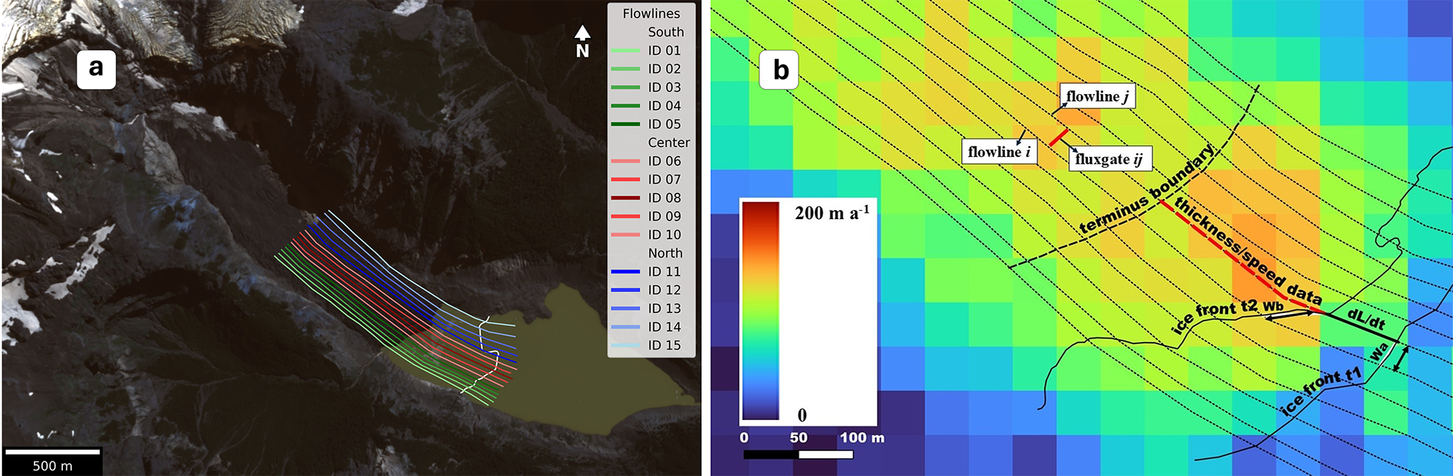
We manually delineated 15 flowlines along the glacier tongue and converted them into multipoint vectors with 3 m vertex spacing. Flowlines were outlined following flow-direction vectors derived from the feature-tracking algorithm (Supplementary Fig. S1a). A comparison with flow vectors from multiple years showed no appreciable offset, indicating that these flowlines remained stable throughout the study period. Each flowline was assigned a unique ID. The two outermost flowlines are located slightly inside the glacier margins to avoid outliers and missing velocity or thickness values, while still capturing the near-marginal flux (Fig. 2a). The number of flowlines was chosen to balance precision and computational cost. With 15 flowlines, the mean spacing is 20–25 m. Given the resolution of the velocity data (60 m for Landsat-derived and 40 m for Sentinel-derived grids), adding more flowlines would provide little additional information while substantially increasing computational cost.
(a) Flowlines used to compute frontal ablation at Manso Glacier. Flowlines are colored by sector with variable tones: green for the southern, red for the central and blue for the northern sector. Background: Pléiades image from 2 March 2020 (© CNES 2012, Airbus DS). Calving front in 2013 outlined in white. (b) Schematic of the multiple fluxgate method. Two flowlines i and j (dotted) follow the ice flow. The fluxgate ij (solid red) is a virtual cross section laterally bounded by these flowlines. Its width w is the average distance between flowlines at the initial (wa) and final (wb) front positions (solid black lines at t 1 and t 2). The dashed red line indicates the segment used to sample ice velocity UT and thickness H (median values). The front displacement rate dL/dt is derived from the front positions. Background: 2017 annual velocity grid (GIV algorithm).

Figure 2 Long description
A) The image shows Manso Glacier with flowlines colored by sector: green for the southern, red for the central, and blue for the northern sector. Fifteen flowlines are labeled from ID 01 to ID 15. A scale bar indicates 500 meters. B) The schematic illustrates the multiple fluxgate method with flowlines i and j following the ice flow. The fluxgate ij is a virtual cross section bounded by these flowlines. The width is the average distance between flowlines at initial and final front positions. The dashed red line indicates the segment used to sample ice velocity and thickness. The terminus boundary and ice front positions are marked. A color gradient represents velocity data from 0 to 200 meters per year, with a scale bar showing 0, 50, and 100 meters. The background features a velocity grid with labeled elements such as thickness/speed data and ice front positions.
3.2. Frontal ablation calculation
Our method begins by computing, for each flowline, the frontal ablation rate ȧ [m a−1 or m d−1] and the ice thickness H [m]. Both variables are derived along the flowline direction.
For each flowline, we track the position of the glacier front between two glacier masks to compute the ice front displacement rate dL/dt. dL is the change in ice front position along the flowline over the temporal interval dt, determined by the dates of both glacier masks.
Frontal ablation rate ȧ is defined as the difference between the depth-averaged ice velocity at the glacier terminus, UT, and dL/dt:
 \begin{equation}\dot a = {U_{\text{T}}} - \frac{{{\text{d}}L}}{{{\text{d}}t}}{\text{ }}\end{equation}
Here, U T is extracted by sampling the velocity field along the flowline and computing the median value over the segment extending from the most retreated front position to a fixed distance upstream to avoid areas where water has replaced ice. This distance was set following a sensitivity analysis to balance proximity to the front with data quality (see Section 3.4.1).
Ice thickness H is obtained as the median of the thickness field sampled along the same flowline segment. Thickness is derived from an initial reference field H 0 (2012) and updated pixelwise using thickness-change rates (dH/dt)n derived from Pléiades surface elevation data. Each (dH/dt)n corresponds to a time interval [tn, tn +1] defined by the acquisition dates of the DEMs used in the differencing. Ice thickness at any target date t is then given by
 \begin{equation}H\left( t \right) = {H_0} + {\sum}_n {(\text{d}H/\text{d}t)_n}\,{\Delta }{t_n}\end{equation}
where Δtn is the fraction of the interval [tn, tn +1] that overlaps with the analysis interval dt.
Two adjacent flowlines i and j define a virtual fluxgate ij, representing a cross-section perpendicular to ice flow (Fig. 2b). The fluxgate width w is computed as the average of the lateral distance between front positions in both flowlines at the start (wa) and end (wb) of the time interval. Accordingly, the fluxgate-averaged frontal ablation rate ȧᵢⱼ and ice thickness Hᵢⱼ are defined as the mean values of ȧ and H along flowlines i and j. For each fluxgate ij, the frontal ablation fa [m3 a−1 or m3 d−1] is computed as
 \begin{equation}f{a_{ij}} = {\dot a_{ij}}\,{H_{ij}}{w }\end{equation}
For n flowlines, the total frontal ablation FA [m3 a−1 or m3 d−1] is computed as the sum of the n − 1 fluxgates:
 \begin{equation}FA = \mathop \sum \limits_{ij = 1}^{n - 1} f{a_{ij}}{\text{ }}\end{equation}
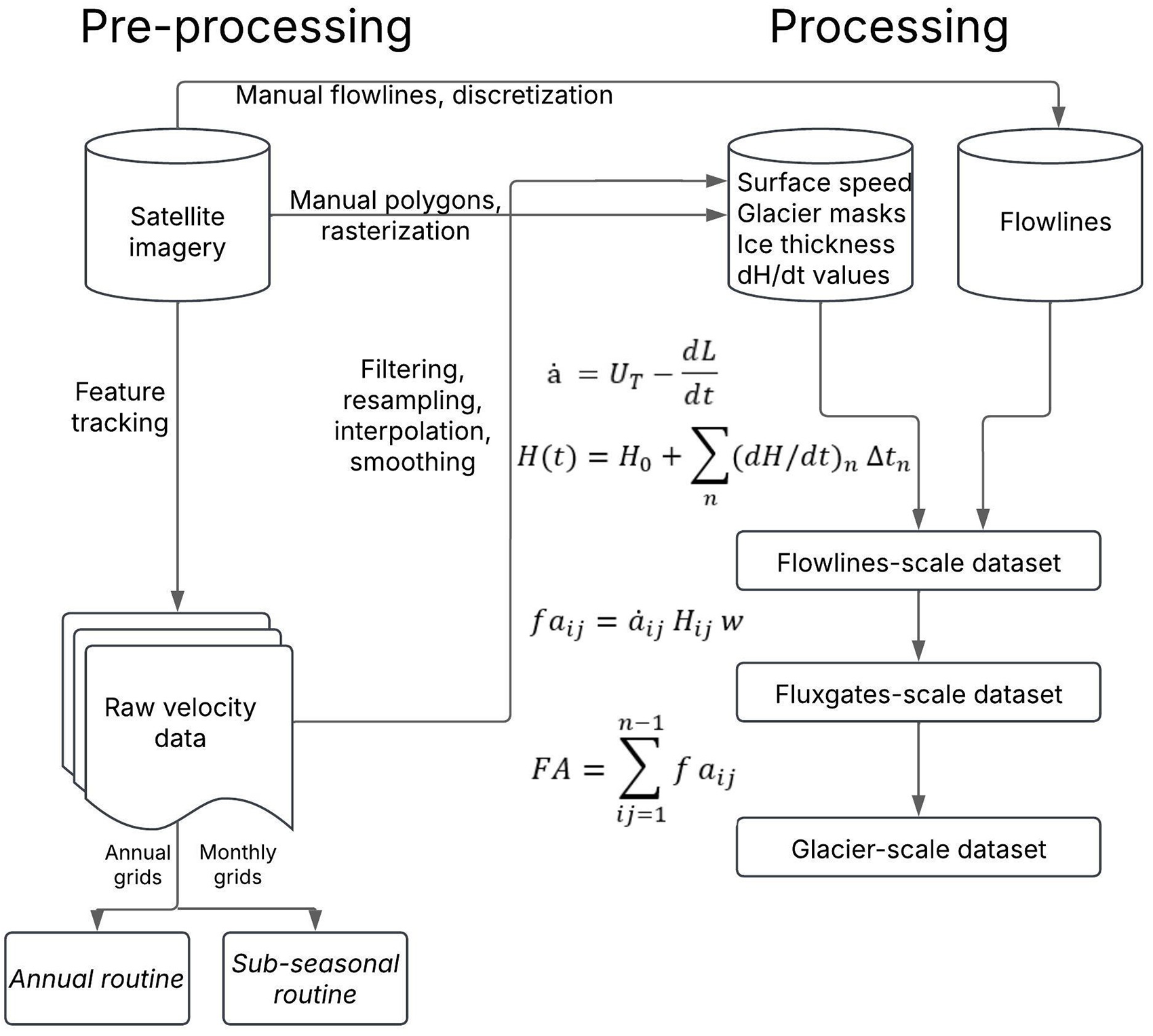
This workflow is implemented as a Python routine (Fig. 3) for the processing stage, encompassing input data handling and retrieval of frontal ablation time series and related variables. The resulting data are available along individual flowlines, fluxgates and for the entire glacier. Building upon this workflow and leveraging the above-calculated velocity grids at monthly and annual scales, we developed routines to estimate frontal ablation at subseasonal and annual scales. Median velocities are used due to their robustness to outliers.
Workflow to compute frontal ablation with the multiple fluxgate method.

Figure 3 Long description
Pre-processing and Processing headings appear at the top. Pre-processing section, left to right and top to bottom. Satellite imagery is shown as a database cylinder. From Satellite imagery, an arrow labeled, Manual flowlines, discretization, goes to Flowlines, shown as a database cylinder on the right side under Processing. From Satellite imagery, an arrow labeled, Manual polygons, rasterization, goes to a process box labeled, Surface speed, Glacier masks, Ice thickness, dH slash dt values. From Satellite imagery, a downward arrow labeled, Feature tracking, goes to Raw velocity data, shown as a stacked document symbol. Under Raw velocity data are two labels, Annual grids, and Monthly grids. From Annual grids, a downward arrow goes to Annual routine. From Monthly grids, a downward arrow goes to Sub-seasonal routine. A vertical line labeled, Filtering, resampling, interpolation, smoothing, connects from the Raw velocity data area toward the Processing section. Processing section, left to right and top to bottom. A process box labeled, Surface speed, Glacier masks, Ice thickness, dH slash dt values, receives the arrow from Manual polygons, rasterization. A separate database cylinder labeled, Flowlines, receives the arrow from Manual flowlines, discretization. Two downward arrows, one from the Surface speed, Glacier masks, Ice thickness, dH slash dt values box and one from the Flowlines cylinder, both point to a process box labeled, Flowlines-scale dataset. A downward arrow from Flowlines-scale dataset points to Fluxgates-scale dataset. A downward arrow from Fluxgates-scale dataset points to Glacier-scale dataset. Equations shown in the Processing section. a hat equals U subscript T minus dL over dt. H of t equals H subscript 0 plus summation over n of open parenthesis dH over dt close parenthesis subscript n times delta t subscript n. f a subscript i j equals a hat subscript i j times H subscript i j times w. FA equals summation from i j equals 1 to n minus 1 of f a subscript i j. No decision points or conditional branches are shown.
Subseasonal analysis intervals dt are defined by specifying a minimum and maximum duration (40–90 days in this study). All possible intervals within this range are generated from the available front positions, and only those containing velocity data are retained. For each interval, velocity is computed as a weighted average of the corresponding monthly grids, with weights proportional to the number of days each month contributes. Ice thickness is updated by integrating the (dH/dt)n values, with Δtn varying according to the overlap between each DEM-derived interval and dt.
Annual intervals dt correspond to the hydrologic year. For each interval, velocity and front positions closest to the start and end dates are used, and ice thickness is updated by integrating the corresponding (dH/dt)n values over the same interval.
3.3. Uncertainty analysis
We first calculated the uncertainties of UT, dL/dt, ȧ and H for each flowline and then propagated them to estimate the final uncertainty for the entire calving front.
For the ice velocity at the glacier terminus, we followed the conventional method to estimate σUT in the raw velocity grids, as the Normalized Median Absolute Deviation (NMAD) of the values of the pixels in motionless ice-free zones (Zheng and others, Reference Zheng2023). The uncertainty of the ice front displacement rate, σdL/dt, is determined by the pixel size of the satellite imagery (Landsat: 15 m; Sentinel: 10 m), as the ice-front positions were manually outlined from them. The error of the frontal ablation rate σȧ is then computed as
 \begin{equation}\begin{array}{*{20}{c}}
{\sigma _{\dot a}} = \sqrt{\sigma _{{U_T}}^2 + \sigma _{{\text{d}}L/{\text{d}}t}^2}
\end{array}\end{equation}
Ice thickness uncertainty arises from two sources: the initial thickness grid σH 0 and the thickness-change rates σ(dH/dt). We adopt the RMSE reported by Zorzut and others (Reference Zorzut, Ruiz, Rivera, Pitte, Villalba and Medrzycka2020) for σH 0 (31 m). For each thickness-change interval (dH/dt)n, the uncertainty σ(dH/dt)n is estimated as the NMAD of stable-terrain pixels (Table 2). Assuming independence, the propagated uncertainty at time t is
 \begin{equation}{\sigma _{H\left( t \right)}} = \sqrt{\sigma _{{H_0}}^2 +\mathop{\sum}\limits_{i}(\sigma _{\text{d}h/\text{d}t,n}^2 \Delta t_n^2)}\end{equation}
where Δtn is the portion of interval [tn, tn +1] contributing to H(t).
At the fluxgate level, we calculate uncertainties of ȧij, Hij and w. We consider that the errors from the neighboring flowlines i and j are spatially correlated by a coefficient ρ that can range between 0 (uncorrelated) and 1 (fully correlated). Conservatively, we assume ρ = 0.5:
 \begin{equation}{\sigma _{\dot a}}_{{ij}} = {\sigma _{{\dot a}}}_{i}\sqrt{\frac{{1 + \rho }}{2}} \end{equation}
 \begin{equation}{\sigma _{{H_{ij}}}} = {\sigma _{{H_i}}}\sqrt {\frac{{1 + \rho }}{2}} {\text{ }}\end{equation}
The uncertainty in the fluxgate width w arises from two sources: the geometric variability between the two neighboring flowlines and the positional uncertainty of the ice front imposed by the glacier-extent mask resolution. The geometric component is represented by the difference between the two width measurements wa and wb; we quantify it as
 \begin{equation}{\sigma _{geom}} = \frac{{\mid {w_a} - {w_b}\mid }}{2}{\text{ }}\end{equation}
The positional component reflects the uncertainty in the location of the calving front, which we approximate as half a pixel of the glacier-extent mask:
 \begin{equation}{\sigma _{pos}} = \frac{{{\text{mask pixel size}}}}{2}{\text{ }}\end{equation}
Assuming both sources are independent, the total uncertainty in σw is
 \begin{equation}{\sigma _w} = \sqrt {\sigma _{geom}^2 + \sigma _{pos}^2} {\text{ }}\end{equation}
Following the propagation rules, we compute the uncertainty of the frontal-ablation flux σfa [V/t] for a single fluxgate ij as
 \begin{equation}
{\sigma _{fa}} = fa\sqrt{{{\left({\frac{{\sigma _{{H_{ij}}}}}{{H_{ij}}}}\right)}^2}{{\left( {\frac{{\sigma {{{{\dot a}}}_{ij}}}}{\dot a_{ij}}}\right)}^2}{{\left( {\frac{{{\sigma _w}}}{w}} \right)}^2}}
\end{equation}
assuming that the individual error sources (ȧij, Hij and w) are statistically independent. Finally, we compute the error of the frontal-ablation rate σFA [V/t] for a given period as
 \begin{equation}{\sigma _{FA}} = \sqrt {\mathop \sum \limits_1^{n - 1} {{\left( {{\sigma _{fa}}} \right)}^2}} {\text{ }}\end{equation}
Uncertainties of individual flux gates are assumed to be independent for the purpose of first-order error propagation.
3.4. Parameter settings
3.4.1. Terminus upstream boundary
To compute frontal ablation as close as possible to the calving front while retaining reliable velocity and thickness data, we defined the near-terminus region and performed a sensitivity analysis on its upstream limit. We tested six distances from the terminus (30, 45, 60, 75, 99 and 120 m), over which velocity and thickness fields were averaged to compute annual frontal ablation. Frontal ablation proved highly insensitive to this parameter: analysis of variance revealed no significant differences among the series, and Tukey’s honestly significant difference test confirmed that all pairwise comparisons were nonsignificant. Variations remained below 5% across the entire tested range. Moreover, the uncertainty envelope of the 75 m series fully contains all other estimates (Supplementary Fig. S3). To ensure inclusion of two velocity pixels from the ice front, we adopt 75 m as the upper boundary of the near-terminus region.
3.4.2. Velocity scaling factor
The relationship between the surface velocity U S and the depth-averaged ice velocity at the glacier terminus U T is commonly expressed through a scaling factor γ, which reflects the combined contributions of internal deformation and basal sliding (Cuffey and Paterson, Reference Cuffey and Paterson2010):
 \begin{equation}{U_T} = \gamma \,{U_{\text{S}}}{\text{ }}\end{equation}
For mountain glaciers, typical values range between 0.8 (purely deformation-driven flow) and values approaching 1 under sliding-dominated, plug-flow conditions (e.g. McNabb and others, Reference McNabb, Hock and Huss2015; Minowa and others, Reference Minowa, Schaefer, Sugiyama, Sakakibara and Skvarca2021; Kochtitzky and others, Reference Kochtitzky2022).
For Monte Tronador, Zorzut and others (Reference Zorzut, Ruiz, Rivera, Pitte, Villalba and Medrzycka2020) estimated the basal-to-surface velocity ratio (UB/Us) through an iterative inversion constrained by GPR-derived ice thickness. In the debris-covered tongue of Manso Glacier, this ratio increases toward the terminus and reaches 0.997 at the calving front, indicating near plug-flow conditions. Under such conditions, the column-averaged velocity closely approaches the surface velocity, and (UB/Us) provides a direct constraint on γ. Accordingly, we adopt γ = 0.997 at the terminus.
3.4.3. Subseasonal interval duration
The duration of the intervals used to compute subseasonal frontal ablation depends on the availability of satellite imagery, its spatial resolution and the glacier’s frontal displacement rate. These factors define a trade-off between temporal resolution and the SNR of the resulting time series. The minimum interval length is critical: short intervals risk being at the limit of spatial resolution, where noise can mask the signal. Although the maximum interval length is not a strict constraint, we set a 90 day upper bound to preserve subseasonal variability. We evaluated the effect of shorter intervals by comparing frontal-ablation datasets computed with varying minimum durations. This inspection revealed that intervals shorter than 40 days led to an increasing number of flowlines exhibiting negative frontal ablation rates, which is physically impossible. Therefore, we defined 40 days as the minimum span.
3.5. Environmental data
To explore potential mechanisms driving variability in frontal ablation, we collected several environmental datasets, including  $T_{air}^\circ $, PP, lake surface temperature (LST) and proglacial lake level.
3.5.1.  $T_{air}^\circ $ and PP

We obtained daily  $T_{air}^\circ $ and PP records since 2014 from an Automatic Weather Station (AWS) installed 6.5 km down-valley (Fig. 1b). PP measurements correspond to rainfall only.
3.5.2. Lake surface temperature
LST was derived from the surface temperature product (ST_B10, 30 m resolution) of Landsat-8 and -9 Collection 2 Level 2, which provides atmospherically corrected land surface temperatures. Over water bodies, this product represents the skin temperature of the water surface (<500 μm) (Oesch and others, Reference Oesch, Jaquet, Hauser and Wunderle2005). After filtering out scenes affected by clouds or fog over the lake, 69 cloud-free images from 2014 to 2024 were retained.
To determine representative LST values, we compared the median temperature of pixels within three lake regions: the entire lake, a zone proximal to the calving front (within 180 m, updated annually) and a distal zone near the Manso River headwaters. Nonparametric tests (Friedman and paired Wilcoxon) indicate that the proximal zone is significantly colder, whereas the distal zone does not differ from the lake-wide average. As correlations with  $\dot a$ were nearly identical among regions, we adopt the median LST from the proximal zone, which is most physically relevant to ice–lake interactions.
Icebergs and seasonal lake ice were not explicitly masked; thus, LST may represent a conservative estimate of open-water surface temperature during periods of partial or complete ice cover. To minimize mixed-pixel effects, a 50 m internal buffer was applied to the lake mask prior to LST extraction.
3.5.3. Lake level
Proglacial lake-level measurements were obtained from the Sistema Nacional de Información Hídrica (Secretaría de Recursos Hídricos, 2025). Data are updated every 4 hours and have been available since September 2021, although some gaps exist.
3.6. Statistical analysis
To assess whether frontal dynamics differ significantly among glacier sectors, flowlines were grouped into southern (IDs 1–5), central (IDs 6–10) and northern (IDs 11–15) sectors. We calculated differences among sectors in UT, dL/dt and ȧ at both subseasonal and annual timescales. Overall differences among sectors were first assessed using the Kruskal–Wallis test. When significant, pairwise contrasts between sectors were evaluated using Mann–Whitney U tests. These nonparametric approaches do not assume normality nor homoscedasticity and are well suited for analyzing spatially heterogeneous datasets (Helsel and others, Reference Helsel, Hirsch, Ryberg, Archfield and Gilroy2020).
4. Results
4.1. Subseasonal frontal ablation 2017–24
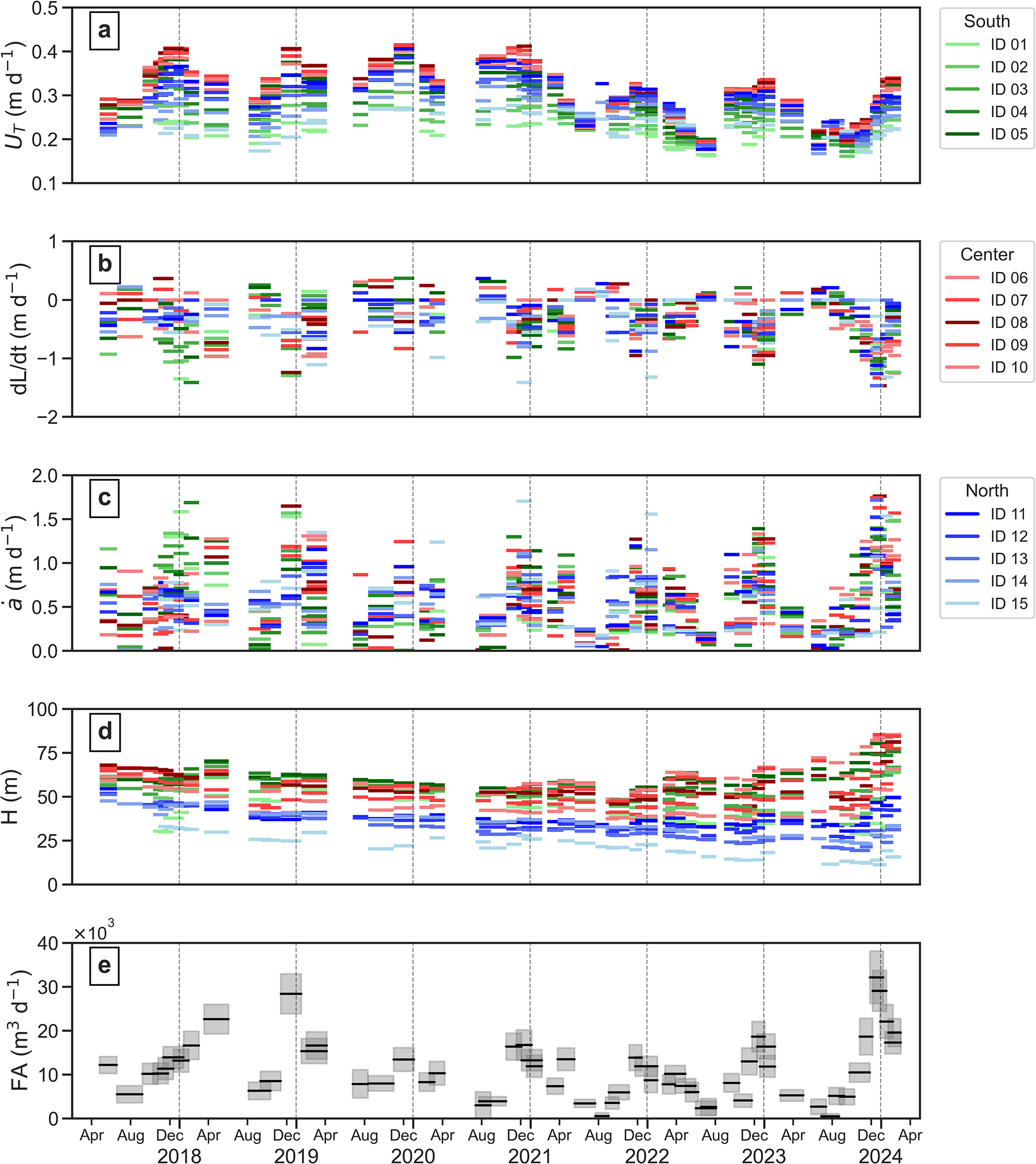
Given the availability of Sentinel-2 data on Patagonia from 2017 onward, we computed frontal ablation at the subseasonal scale between April 2017 and April 2024. Ice velocity at the glacier terminus UT (Fig. 4a) and ice front displacement rate dL/dt (Fig. 4b) exhibit clear seasonal cycles, with maxima in summer (December–February) and minima in winter (June–August). Frontal ablation rate ȧ follows the same pattern, with values near 0 m d−1 in winter and peaks in summer (Fig. 4c).
Subseasonal time series of ice velocity at the glacier terminus (a), ice front displacement rate (b), frontal ablation rate (c), ice thickness (d) and glacier-wide frontal ablation (e) between April 2017 and April 2024. Panels (a)–(d) show flowline-level variability, with southern flowlines in green tones, central in red and northern in blue, while panel (e) integrates these components at the glacier scale (shaded areas indicate uncertainty). Note the varying Y-axis scales in panels (a)–(c). Dashed gray lines separate years.

Figure 4 Long description
The time series plot labeled, a, of terminus velocity is shown in image A. The y-axis label is, U subscript T, with unit, meters day superscript minus 1. The y-axis ranges from 0.1 to 0.5 with ticks at 0.1, 0.2, 0.3, 0.4, and 0.5. The x-axis shows time with repeating month labels, Apr, Aug, Dec, and Apr, and year labels, 2018, 2020, 2022, and 2024. Vertical dashed lines separate year blocks. A legend lists South IDs, ID 01, ID 02, ID 03, ID 04, and ID 05. Data are shown as short horizontal segments at many dates. Values are mostly between about 0.2 and 0.4, with several clusters near 0.4 around multiple Dec positions and several clusters nearer 0.2 around multiple Aug positions. The time series plot labeled, b, of ice front displacement rate is shown in image B. The y-axis label is, dL slash dt, with unit, meters day superscript minus 1. The y-axis ranges from minus 2 to 1 with ticks at minus 2, minus 1, 0, and 1. The x-axis shows time with repeating month labels, Apr, Aug, Dec, and Apr, and year labels, 2018, 2020, 2022, and 2024, with vertical dashed year separators. A legend lists Center IDs, ID 06, ID 07, ID 08, ID 09, and ID 10. Data are short horizontal segments. Values are mostly between about minus 1.5 and 0.5, with many segments below 0 across the record and several clusters extending below minus 1 toward later dates. The time series plot labeled, c, of frontal ablation rate is shown in image C. The y-axis label is, a with overdot, with unit, meters day superscript minus 1. The y-axis ranges from 0.0 to 2.0 with ticks at 0.0, 0.5, 1.0, 1.5, and 2.0. The x-axis shows time with repeating month labels, Apr, Aug, Dec, and Apr, and year labels, 2018, 2020, 2022, and 2024, with vertical dashed year separators. A legend lists North IDs, ID 11, ID 12, ID 13, ID 14, and ID 15. Data span from near 0.0 up to near 2.0, with repeated clusters around 0.5 to 1.5 and several higher segments near 1.5 to 2.0 near the end of the record. The time series plot labeled, d, of ice thickness is shown in image D. The y-axis label is, H, with unit, meters. The y-axis ranges from 0 to 100 with ticks at 0, 25, 50, 75, and 100. The x-axis shows time with repeating month labels, Apr, Aug, Dec, and Apr, and year labels, 2018, 2020, 2022, and 2024, with vertical dashed year separators. Data are short horizontal segments. Values commonly fall between about 20 and 80, with many segments around 40 to 60 earlier in the record and a wider spread later, including segments near 70 to 80 near the end. The time series plot labeled, e, of frontal ablation is shown in image E. The y-axis label is, FA, with unit, meters superscript 3 day superscript minus 1, and a multiplier, times 10 superscript 3, is shown near the y-axis. The y-axis ranges from 0 to 40 with ticks at 0, 10, 20, 30, and 40. The x-axis shows time with repeating month labels, Apr, Aug, Dec, and Apr, and year labels, 2018, 2020, 2022, and 2024, with vertical dashed year separators. Data are shown as shaded rectangular boxes with a darker horizontal line inside each box. Values include boxes near about 5 to 15 early in the record, several boxes around 20 to 30 at various times, and a cluster near the end reaching into the 30 to 40 range.
Spatially, UT shows the most persistent spatial pattern, with the central sector consistently fastest across most of the record, followed by the northern and southern sectors. Kruskal–Wallis tests (p < 0.05) are significant in most of the 58 subseasonal intervals, with pairwise Mann–Whitney U tests indicating that the central sector frequently differs from the other two. In contrast, dL/dt exhibits higher spatial dispersion within each interval (average inter-flowline SD ∼0.35 vs 0.06 m d−1 for UT), and ȧ shows the highest temporal and spatial variability.
The locations of maximum ȧ shifted across the glacier front throughout the study period. Peaks occurred in the southern sector in summer 2017/18 (∼1.58 m d−1), in the southern and central sectors in 2018/19 (∼1.57 and ∼1.64 m d−1) and in the northern sector in late winter/spring 2021 (∼0.85 m d−1) and summer 2021/22 (∼1.56 m d−1). Additional peaks were observed in the central sector in late 2019 (∼1.24 m d−1) and most prominently in summer 2023/24 (∼1.76 m d−1, the absolute maximum recorded).
Temporal trends show deceleration after 2021, with seasonal maxima of UT decreasing from ∼0.40 to ∼0.33 m d−1 and seasonal minima from ∼0.20 to ∼0.17 m d−1. Maximum advance of dL/dt reaches ∼0.37 m d−1 and maximum retreat ∼1.45 m d−1.
Terminus thickness exhibits a marked spatial variability across the calving front, with generally thicker ice in the central and southern sectors and thinner ice toward the northern margin Fig. 4d).
Glacier-wide subseasonal frontal ablation shows a seasonal pattern consistent with ȧ (Fig. 4e), with absolute minima in winter 2022 (∼2600 m3 d−1) and peaks in fall 2018 (∼22 600 m3 d−1), summer 2018/19 (∼28 350 m3 d−1) and summer 2023/24 (∼32 100 m3 d−1). A sharp decline occurred in summer 2019/20 (∼13 200 m3 d−1), followed by relatively low values in summers 2020/21–2022/23 (∼16 300–16 700 m3 d−1).
4.2. Annual frontal ablation 2013–23
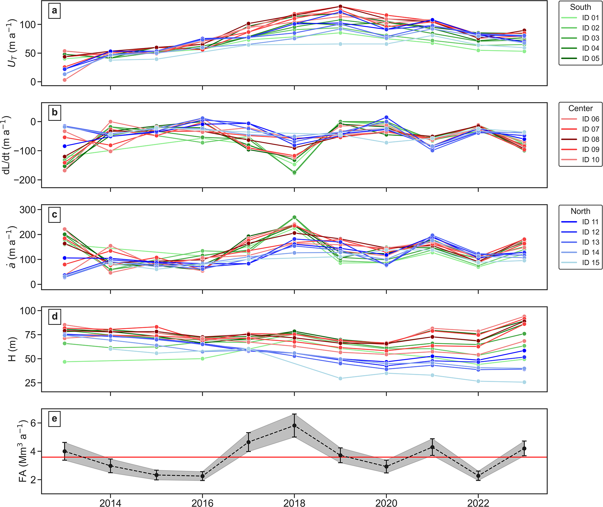
At the annual timescale, we extended the dataset to span a full decade (2013–23) by integrating Landsat- and Sentinel-derived data (Fig. 5). Frontal ablation rate resembles the pattern of ice front displacement rates, generally greater than ice velocities at the glacier terminus.
Annual time series at the flowline level of ice velocity at the glacier terminus (a), ice front displacement rate (b), frontal ablation rate (c) and ice thickness (d) between 2013 and 2023, with southern, central and northern flowlines shown in green, red and blue tones, respectively. Panel (e) shows annual frontal ablation. Shaded areas and error bars indicate uncertainty, and the red line represents the 2013–23 mean (∼3.6 Mm3 a−1).

Figure 5 Long description
The multi-line graph consists of five panels comparing ice dynamics from 2013 to 2023 across different flowlines. The x-axis represents years from 2013 to 2023. Panel A shows ice velocity, U subscript T, meter a superscript minus 1, with southern flowlines in green, central in red, and northern in blue. The lines generally increase over time, with notable peaks around 2018 and 2022. Panel B displays ice front displacement rate, dL over dt, meter a superscript minus 1, with similar flowline color coding. The lines fluctuate, with a significant dip around 2016. Panel C illustrates frontal ablation rate, a dot, meter a superscript minus 1, showing varied trends with peaks around 2018. Panel D presents ice thickness, H, meter, with consistent values across years, lacking specific group identification. Panel E shows frontal ablation, FA, Mm superscript 3 a superscript minus 1, with a dashed line indicating annual values, a shaded band for uncertainty, and a horizontal line representing the mean. The graph highlights differences in ice dynamics across regions, emphasizing variability and trends over the decade.
UT increased across most flowlines until 2019, particularly in the central sector (∼130 m a−1), and decreased thereafter, stabilizing around 2022 (Fig. 5a). dL/dt shows high variability until 2018, with maximum retreats in 2013 and 2018 restricted to southern and northern sectors, and advances in 2016 and 2020 concentrated in the northern sector (Fig. 5b). Absolute maximum retreat exceeds −220 m a−1 (2013), and maximum advances reach ∼15 m a−1.
Spatial patterns are evident among sectors. UT is consistently fastest in the central sector, with Kruskal–Wallis tests significant in 7 of 11 years. dL/dt and ȧ show larger interannual variation in sector dominance, with significant contrasts in 5–6 years.
Peaks of ȧ occur in the southern (2013: 198 m a−1, 2017: 245 m a−1), central (2016: 198 m a−1, 2018: 234 m a−1) and northern sector (2021: 197 m a−1) (Fig. 5c). Terminus thickness (Fig. 5d) shows a spatial pattern consistent with that observed in the subseasonal dataset.
From 2013 to 2023, frontal ablation on Manso Glacier averaged 3.6 ± 0.5 Mm3 a−1 (0.0033 ± 0.0005 Gt a−1 assuming an ice density of 917 kg/m3), with minima in 2015, 2016 and 2022 (2.3 ± 0.3 Mm3 a−1) and a peak in 2018 (5.8 ± 0.8 Mm3 a−1) (Fig. 5e). Over the decade, cumulative frontal ablation loss was 39.5 ± 1.8 Mm3 (0.036 ± 0.002 Gt).
4.3. Error budget of frontal ablation
Frontal ablation uncertainty is primarily controlled by ice thickness, followed by the frontal ablation rate ȧ and fluxgate width w (∼55%, ∼35% and ∼10%, respectively). On an annual scale, the average relative uncertainty is ∼15%, whereas at subseasonal scales it is higher, averaging ∼29%. The larger subseasonal uncertainty reflects the amplification of measurement errors over shorter periods and greater sensitivity to fluctuations in frontal displacement. This balance of contributions remains consistent across temporal scales, highlighting the dominant role of ice thickness.
4.4. Frontal ablation rate and environmental variables
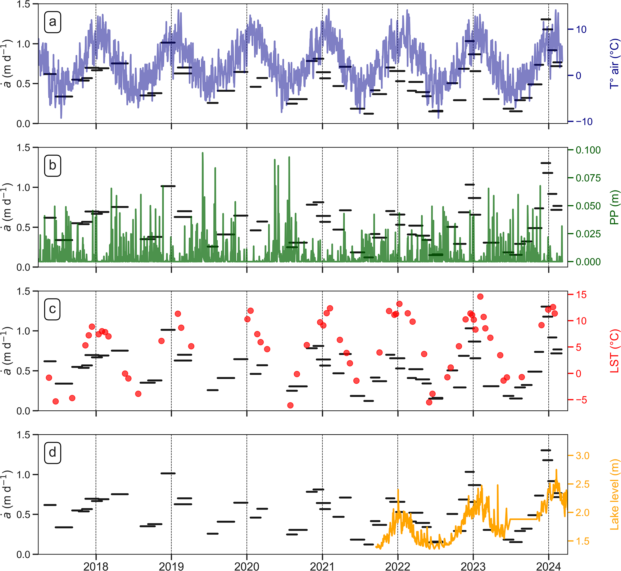
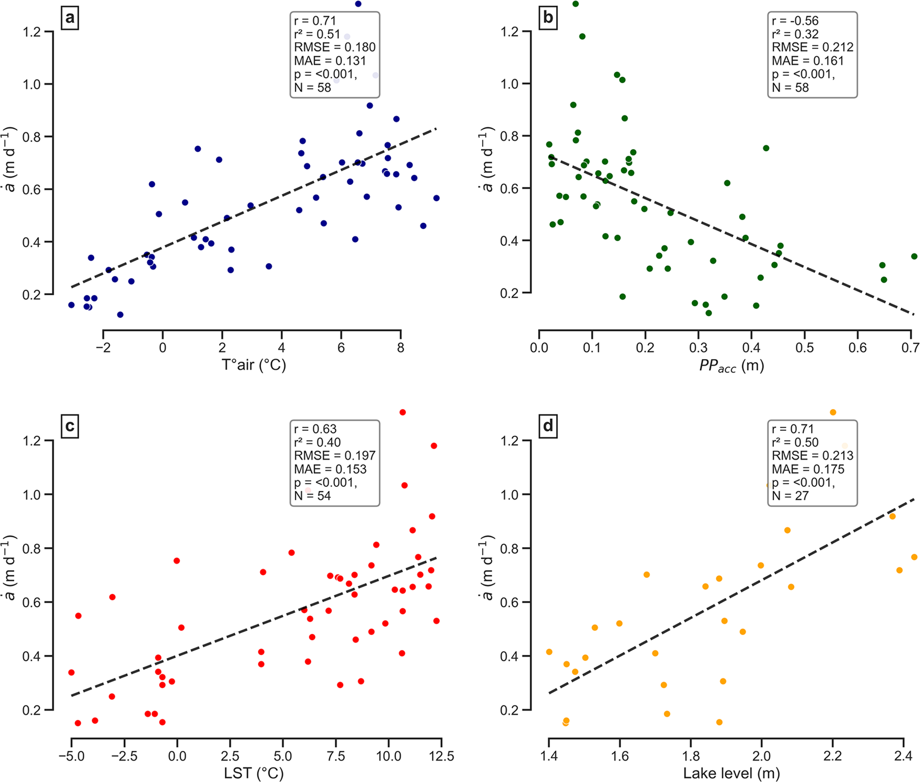
We analyzed the relationship between average ȧ at a subseasonal scale with  $T_{air}^\circ $, PP, LST and lake level (Fig. 6). For each interval in the subseasonal time series, we correlate the average ȧ across all flowlines with the averages of
 $T_{air}^\circ $, LST and lake level within the interval and with the cumulative precipitation (PPacc) in the interval. We used Pearson correlation and least squares regression to estimate linear trends.
Time series of subseasonal frontal ablation rate averaged across all flowlines in black lines and daily  $T_{air}^\circ $ in blue (a), PP in green (b), LST in red dots (c) and lake level in orange (d).

Figure 6 Long description
The graphs compare subseasonal frontal ablation rate, a dot left parenthesis m d superscript minus 1 right parenthesis, with different environmental variables from 2018 to 2024. The horizontal axis is shared across all graphs, representing years 2018 to 2024. The vertical axis for a dot left parenthesis m d superscript minus 1 right parenthesis ranges from 0.0 to 1.5 in all graphs. In graph A, the right vertical axis shows air temperature, T subscript air left parenthesis degree c right parenthesis, ranging from minus 10 to 10. A blue line indicates seasonal cycles in air temperature, with peaks and troughs corresponding to changes in a dot. Black horizontal dash markers represent average ablation rates over specific periods. Graph B displays precipitation, PP left parenthesis m right parenthesis, on the right vertical axis ranging from 0.000 to 0.100. Green spikes indicate episodic precipitation events, with notable high spikes around 2020 and 2022. Black horizontal dash markers show average ablation rates during these events. Graph C shows land surface temperature, LST left parenthesis degree c right parenthesis, on the right vertical axis ranging from minus 5 to 15. Red dots represent LST values, varying over time with higher values around 2021 and 2023. Black horizontal dash markers indicate average ablation rates. Graph D illustrates lake level left parenthesis m right parenthesis, on the right vertical axis with tick labels 1.5, 2.0, 2.5, 3.0. An orange line shows lake level changes, mainly rising after 2022, with peaks near 2024. Black horizontal dash markers denote average ablation rates. The graphs collectively show how changes in air temperature, precipitation, land surface temperature, and lake level relate to subseasonal frontal ablation rates, highlighting periods of higher ablation corresponding to environmental changes.
4.4.1.
$T_{air}^\circ $ and PP

 $T_{air}^\circ $ shows a clear annual cycle, with maxima in January–February exceeding 14°C and minima in June–July dropping below −9°C during the strongest cold spells (Fig. 6a). Seasonal means are ∼7.8°C in summer and ∼−1.9°C in winter. Spring exhibits rapid warming, whereas autumn cooling is more gradual. There is a positive correlation between ȧ and
 $T_{air}^\circ $ (r = 0.71, r 2 = 0.50, p < 0.001; Fig. 7a).
Pearson correlation between the averaged frontal ablation rate per each interval in the subseasonal time series and averaged  $T_{air}^\circ $ (a), PPacc (b), averaged LST (c) and lake level (d). Linear regressions are shown as dashed black lines.

Figure 7 Long description
Four scatter plots labeled a to d, each showing the relationship between frontal ablation rate and different variables. In plot a, the horizontal axis represents air temperature in degrees Celsius, ranging from negative 2 to 8. The vertical axis represents frontal ablation rate in meters per day, ranging from 0.2 to 1.2. The plot shows a positive correlation with a Pearson correlation coefficient of 0.71, indicating that higher temperatures are associated with increased ablation rates. Plot b shows the relationship between frontal ablation rate and accumulated precipitation in meters, ranging from 0.0 to 0.7 on the horizontal axis. The vertical axis remains the same as plot a. This plot shows a negative correlation with a Pearson correlation coefficient of minus 0.56, suggesting that higher precipitation is associated with lower ablation rates. Plot c illustrates the relationship between frontal ablation rate and land surface temperature in degrees Celsius, ranging from negative 5.0 to 12.5 on the horizontal axis. The vertical axis is consistent with previous plots. A positive correlation is observed with a Pearson correlation coefficient of 0.63, indicating that higher land surface temperatures correspond to increased ablation rates. Plot d shows the relationship between frontal ablation rate and lake level in meters, ranging from 1.4 to 2.4 on the horizontal axis. The vertical axis remains unchanged. This plot also shows a positive correlation with a Pearson correlation coefficient of 0.71, suggesting that higher lake levels are associated with increased ablation rates. Each plot includes a dashed regression line representing the linear relationship. The points are color-coded to differentiate the panels, with no additional meaning attributed to the colors. The plots do not show any notable clusters or outliers, and the distribution of points appears relatively uniform across each plot.
Daily PP shows a marked seasonal pattern (Fig. 6b). Winter is the wettest period, with mean daily values around 7.9 mm d−1, and a secondary peak occurs in November (late spring). January is the driest month (∼1–1.5 mm d−1). The series is characterized by many dry days interspersed by short, intense PP events: the maximum reaches 97.3 mm in a day. These events occur predominantly during the cold and transitional seasons, while summer remains comparatively dry. There is a negative correlation between ȧ and PPacc (r = −0.56, r 2 = 0.31, p < 0.001; Fig. 7b).
4.4.2. Lake surface temperature
LST closely follows the atmospheric seasonal cycle with distinct thermal regimes (Fig. 6c). Summer values typically reach ∼10.5°C, with peaks up to ∼14–15°C. In winter, LST frequently drops below −5°C and averages −2.8°C, reflecting partial or complete lake freezing as confirmed by winter satellite imagery. The spring transition marks a rapid shift from frozen to open-water conditions. There is a positive correlation between ȧ and LST (r = 0.63, r 2 = 0.40, p < 0.001; Fig. 7c).
4.4.3. Lake level
Lake level exhibits a strong seasonal signal driven by meltwater inputs, rising through spring and peaking in January–February, with minima around July (Fig. 6d). The annual amplitude ranges from 0.8 to 1 m. Short-lived peaks coincide with individual PP events. A linear trend analysis indicates a significant long-term rise of +0.11 m a−1 (p < 0.001). There is a positive correlation between ȧ and lake level (r = 0.71, r 2 = 0.50, p < 0.001; Fig. 7d).
5. Discussion
5.1. Calving front dynamics
Both subseasonal and annual resolutions reveal a sharp contrast between glacier dynamics and frontal ablation. Ice velocity at the glacier terminus UT maintains a stable spatial pattern largely controlled by valley geometry and ice thickness distribution, with limited temporal variability beyond the multi-year velocity-up until 2019 and subsequent deceleration. Conversely, frontal ablation rate ȧ shows strong spatial and temporal variability.
At the subseasonal scale, ȧ hotspots migrate rapidly and irregularly (Supplementary Fig. S4). Hotspots appear across all sectors under both warm and cold conditions, likely linked to localized processes such as evolving subglacial drainage or structural weakening. At the annual scale, ȧ hotspots alternate through the decade, shifting from southern to northern to central sectors. Similar migration of frontal ablation hotspots is observed in tidewater glacier settings (e.g. Wagner and others, Reference Wagner2019; Downs and others, Reference Downs, Brinkerhoff and Morlighem2023).
Overall, the calving front behaves as a stochastic system (Bassis, Reference Bassis2011; Benn and others, Reference Benn2026) where long-term geometry provides a background structure but does not determine the instantaneous location of frontal ablation hotspots. The multi-flowline approach allows us to track their shifting positions and capture the complexity across the calving front. This is particularly evident under local topographic and mechanical controls.
For instance, asymmetric retreat and flotation transitions following the loss of a basal pinning ridge are observed at Perito Moreno Glacier (Koch and others, Reference Koch2025), partially floating termini can persist alongside grounded margins at Mendenhall Glacier (Boyce and others, Reference Boyce, Motyka and Truffer2007) and decoupled retreat of main tongues after tributary disconnection occurs at Upsala Glacier (Lo Vecchio and others, Reference Lo Vecchio, Villalba, Falaschi, Ruiz, Vacaflor and Vargas2025). These examples show how local controls produce spatially heterogeneous frontal-ablation patterns that would remain obscured in single fluxgate estimates.
5.2. Controls of calving front position
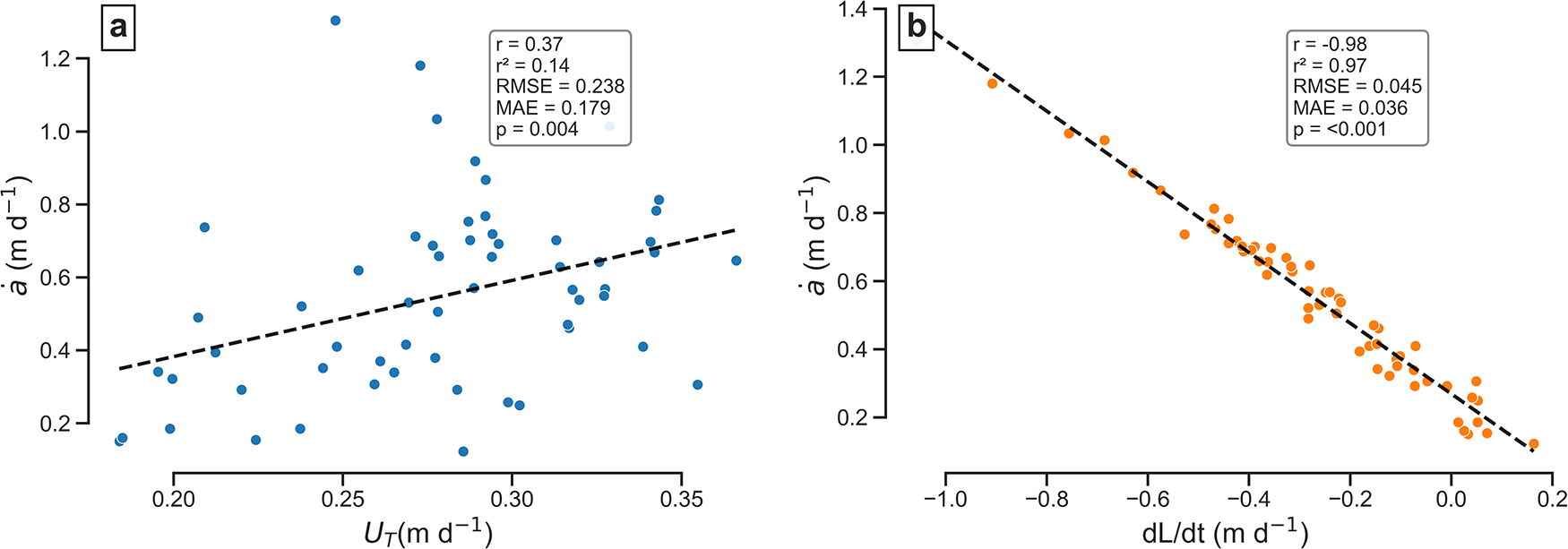
At the subseasonal scale, we correlated the average frontal ablation rate per interval with both UT and dL/dt. While no significant correlation was found between ȧ and UT (r = 0.38, r 2 = 0.14, p = 0.004; Fig. 8a), a strong negative correlation was observed between ȧ and dL/dt (r = −0.98, r 2 = 0.97, p < 0.001; Fig. 8b). Because frontal ablation rates are consistently at least two to three times greater than ice velocity at the glacier terminus, glacier front position appears to be controlled primarily by frontal ablation rather than by ice flow. A similar pattern was reported at Perito Moreno Glacier (SPI) by Minowa and others (Reference Minowa, Sugiyama, Sakakibara and Skvarca2017).
Pearson correlation between the averaged frontal ablation rate per interval in the subseasonal frontal ablation time series with averaged ice velocity at the glacier terminus (UT) (a) and averaged ice front displacement rate (dL/dt) (b). Linear regressions are shown as dashed black lines.

Figure 8 Long description
Scatter plot illustrating the relationship between UT and a dot a. The horizontal axis represents UT in meters per day, ranging from 0.20 to 0.35. The vertical axis represents a dot a in meters per day, ranging from 0.2 to 1.2. The plot shows a weak positive correlation, with points scattered and a dashed line indicating the trend. The text box provides correlation statistics: r equals 0.37, r superscript 2 equals 0.14, RMSE equals 0.238, MAE equals 0.179, p equals 0.004. Points are distributed without significant clustering or outliers. Scatter plot illustrating the relationship between dL over dt and a dot a. The horizontal axis represents dL over dt in meters per day, ranging from negative 1.0 to 0.2. The vertical axis represents a dot a in meters per day, ranging from 0.2 to 1.4. The plot shows a strong negative correlation, with points densely clustered along the dashed trend line, particularly around mid-range x values. The text box provides correlation statistics: r equals minus 0.98, r superscript 2 equals 0.97, RMSE equals 0.045, MAE equals 0.036, p equals less than 0.001. The orange points do not indicate categorical differences. Panel C is not present in the image.
5.3. Correlation of frontal ablation rate and environmental variables
5.3.1.
$T_{air}^\circ $ and PP

The strong correlation between ȧ and  $T_{air}^\circ $ (r = 0.71) is comparable to the value reported for Perito Moreno Glacier (r = 0.86, Minowa and others, Reference Minowa, Sugiyama, Sakakibara and Skvarca2017) and could be explained by enhanced surface melt during warmer periods, which increases subglacial water input and reduces basal friction, thereby accelerating ice flow at the terminus (e.g. Copland and others, Reference Copland, Sharp and Nienow2003; Bartholomaus and others, Reference Bartholomaus, Anderson and Anderson2008; Vincent and Moreau, Reference Vincent and Moreau2016).
The negative correlation with PPacc (r = −0.56) likely reflects the seasonal distribution of PP in Patagonia. Although PP is recorded as rainfall at the AWS, it likely falls predominantly as snow at the glacier tongue altitude during winter, when subglacial drainage is largely inactive (Hoffman and Price, Reference Hoffman and Price2014; Rada Giacaman and Schoof, Reference Rada Giacaman and Schoof2023).
At Manso Glacier, the maximum correlation between ȧ and  $T_{air}^\circ $ occurs with no detectable lag. This suggests that frontal ablation remains closely coupled to contemporary climatic forcing. Under the observed trend of increasing
 $T_{air}^\circ $ and decreasing PP in Northern Patagonia (Salazar and others, Reference Salazar, Thatcher, Goubanova, Bernal, Gutiérrez and Squeo2024), continued atmospheric warming would likely intensify frontal ablation through enhanced meltwater input to the subglacial drainage system. Further warming could also shift a larger fraction of winter PP from snow to rain, potentially increasing liquid input to the glacier bed.
Ice thickness increased along the entire calving front since 2023. A plausible interpretation is that frontal retreat has positioned the terminus within a bedrock depression where ice is thicker, potentially exposing the calving front to deeper water. If correct, this topographic setting could promote enhanced basal sliding, decreasing the sensitivity of frontal ablation to climatic forcing in the future.
5.3.2. Lake surface temperature
The moderate correlation between ȧ and LST (r = 0.63) indicates a secondary influence on subseasonal terminus dynamics, weaker than in the SPI. At Perito Moreno Glacier, Minowa and others (Reference Minowa, Sugiyama, Sakakibara and Skvarca2017) reported a much stronger correlation of frontal ablation with lake-water temperature (r = 0.95, depth < 2 m) attributed to enhanced subaqueous melt, with vertical profiles confirming the thermal structure of the lake. They also documented a ∼1 month lag between upper lake temperature and  $T_{air}^\circ $. Dye and others (Reference Dye, Bryant, Dodd, Falcini and Rippin2021) showed that Landsat-derived LST closely tracks these near-surface in situ temperatures (r = 0.93), supporting its use as a proxy for surface layer conditions.
Sugiyama and others (Reference Sugiyama and Minowa2016, Reference Sugiyama2021) showed that large proglacial lakes in SPI are typically stratified with a wind-mixed, relatively warm surface layer, overlying a colder, denser layer dominated by subglacial discharge. Subaqueous melt occurs primarily within this upper layer, while deeper cold water limits heat transfer to the terminus. Thus, LST likely reflects the thermal state of the surface layer that is most relevant for frontal melt variability.
At Manso Glacier, LST and  $T_{air}^\circ $ are strongly correlated, and the lake shows a shorter thermal response time, with cross-correlation indicating a ∼2 week lag (r = 0.92). This lag should be viewed cautiously because the sparse and irregular sampling of LST can introduce artifacts. The small area of Lago Manso (0.93 km2 in 2024) likely favors rapid adjustment of the surface layer to atmospheric forcing, with efficient mixing and less persistent stratification than in larger SPI lakes.
Given the available LST dataset, the relative contributions of lake thermal conditions and atmospheric forcing cannot be fully disentangled. Nevertheless, the observed correlations suggest that lake thermal conditions modulate subseasonal frontal ablation variability at Manso Glacier. Thermal structure and circulation of the lake remain unexplored; targeted field measurements such as vertical temperature profiles are needed to quantify subaqueous melt and better constrain the coupling between atmospheric forcing, lake dynamics and calving processes.
5.3.3. Lake level
The strong correlation between ȧ and lake level (r = 0.71) likely reflects seasonal hydrological input to the proglacial lake rather than direct mechanical control on calving. Higher lake levels are associated with increased meltwater availability and coincide with periods of enhanced frontal ablation.
Buoyancy-driven calving under the observed conditions is unlikely: following a height above buoyancy criterion (Van der Veen, Reference Van der Veen1996; Benn and others, Reference Benn, Warren and Mottram2007), flotation would require a freeboard of ∼6 m, whereas the actual freeboard at the terminus is on the order of ∼35 m. The total ice thickness at the glacier terminus is ∼65 m, and the lake depth close to the calving front is ∼30 m. Satellite imagery also shows no evidence of large basal detachment events or unusually large icebergs. These observations suggest that lake level primarily reflects glacial meltwater input.
5.4. The role of SMB
The influence of SMB on our method is minimized by computing frontal ablation from a near-terminus zone extending from the calving front up to 75 m upstream (Section 3.4.1). Ice traverses this distance in ∼250 days at the mean annual terminus velocity (∼110 m a−1), and the resulting near-terminus area (∼30 000 m2, ∼400 m average front width) strongly limits potential volume loss associated with SMB.
In situ SMB measurements from ablation stakes located ∼1 km upstream of the terminus (Section 3.1.1) indicate mean values of ∼12 m w.e. a−1 in recent years, representative of strong ablation conditions in the lower glacier. Although spatial variability is expected in this debris-covered terminus region, these values provide a reasonable upper bound for local SMB. Converting this rate to ice volume over the near-terminus area yields ∼0.39 Mm3 a−1, equivalent to ∼11% of the mean annual frontal ablation (3.6 ± 0.5 Mm3 a−1), and therefore within the ∼15% uncertainty of the annual estimates (Section 4.3).
Observed near-terminus ice thickness changes (dH/dt) average −7.5 m a−1, with a maximum of −9.88 m a−1 (2017–18, Table 2). The discrepancy between these values and the higher SMB rates (∼−13 m a−1) of ice implies a positive emergence velocity of ∼5–6 m a−1. According to mass continuity (Cuffey and Paterson, Reference Cuffey and Paterson2010), near-terminus SMB is therefore partially offset by vertical ice flux associated with flow divergence.
Even under extreme conditions where SMB could reach ∼15–16 m w.e. a−1 over the terminus, the resulting volume loss would still lie within the 15% uncertainty of the annual frontal ablation estimates. At subseasonal timescales, where uncertainty rises (∼30%), the relative contribution of SMB is smaller, as individual ice parcels traverse only a fraction of the near-terminus domain during short intervals.
5.5. Limitations of frontal ablation calculation
The temporal resolution of the multiple fluxgate method strongly depends on velocity data and glacier mask grids. Accurate velocities for a given period require a high SNR for the expected displacement. The SNR depends on both the cross-correlation and filtering method and the quality of the images, including spatial-temporal resolution, georeferencing and orthorectification (Heid and Kääb, Reference Heid and Kääb2012).
We used the GIV algorithm with the panchromatic band (B8) on Landsat-8 (spatial resolution: 15 m, temporal resolution: 16 days) and the near-infrared (NIR: B5) band on Sentinel-2 (spatial resolution: 10 m, temporal resolution: 5 days), as suggested for feature tracking by previous studies (e.g. Kääb and others, Reference Kääb, Winsvold, Altena, Nuth, Nagler and Wuite2016) (see Table 1 and Supplementary Fig. S5). Although GIV does not perform automatic co-registration, Landsat Collection 2 and Sentinel-2 L1C products distributed through Google Earth Engine are already orthorectified and internally co-registered by their providers (ESA, 2015; Crawford and others, Reference Crawford2023).
For Landsat-7 and -8 (2013–15), an average of 13–14 images per year were available, yielding reliable annual velocities. However, the coarser resolution and longer revisit time of Landsat prevented realistic monthly grids. Sentinel-2 (2016–24) provided an average of 29 images per year, allowing higher-quality annual velocity grids, and reliable monthly velocities were possible starting in 2017. Maximum coverage in this region was reached in March 2017, with the launch of Sentinel-2B (Troilo and others, Reference Troilo, Dematteis, Zucca, Funk and Giordan2024). Testing GIV with Landsat-7 TOA alone was not feasible due to image scarcity and Scan Line Corrector failure gaps (Storey and others, Reference Storey2005). In 2013, Landsat-7 and -8 TOA were used together to improve coverage.
Due to its small size and relatively slow ice flow, Manso Glacier exhibits surface displacements only slightly above the resolution of the velocity data: 60 m for Landsat-derived and 40 m for Sentinel-derived grids. This implies a relatively low SNR, and when two images are acquired close in time, feature displacements can be comparable to noise (Millan and others, Reference Millan2019). Winter conditions, with thick cloud cover and surface snow, further reduce the number of images available for correlation. We tested combining Landsat and Sentinel-2 scenes, but this approach was discarded because the sensors have different spatial resolutions and are not co-registered between each other, producing velocity grids with excessive noise compared to those derived from Sentinel-2 alone.
All velocity grids were visually inspected, which was essential for winter scenes where validation was not possible. Only grids showing coherent flow patterns, such as acceleration near the calving front, lower velocities at the margins and maximum ice velocity at the cliff wall, were retained.
Troilo and others (Reference Troilo, Dematteis, Zucca, Funk and Giordan2024) applied the GIV algorithm to Sentinel-2 images of valley glaciers in the Alps, obtaining reliable monthly grids for glaciers with velocities exceeding 40 m a−1. Given Manso Glacier’s average annual velocity of 90–100 m a−1, we are confident in using these monthly grids for subseasonal frontal ablation. Our grids had an average error of 12.6 m a−1, similar to the ∼11 m a−1 reported by these authors. However, measuring velocity outside the glacier may overestimate error due to movements of trees, hillside shifts and shadows (Nanni and others, Reference Nanni, Scherler, Ayoub, Millan, Herman and Avouac2023).
Estimating ice front displacement rates remains a major limitation for computing subseasonal frontal ablation, as it relies on image georeferencing and spatial resolution. Comparing Landsat-8 with Sentinel-2 optical images during manual digitization revealed differences in georeferencing accuracy. Unlike Landsat, which uses numerous ground control points (GCPs) and DEMs, Sentinel-2 employs an automated GCP identification approach (ESA, 2015), introducing slight misregistration errors. Georeferencing improved with the Global Reference Image dataset but still does not match Landsat (CE90 <6 m vs <3 m) (Rengarajan and others, Reference Rengarajan, Choate, Hasan and Denevan2024).
Another source of misregistration arises from using a static DEM for orthorectification, which does not account for temporal glacier surface changes. Although the availability of global DEMs has improved in recent years (e.g. TanDEM-X and Copernicus GLO-30), lateral offsets of up to ∼1 pixel remain common over glaciers because DEMs are often outdated relative to image acquisition and ongoing surface lowering persists. This effect increases with off-nadir distance (Kääb and others, Reference Kääb, Winsvold, Altena, Nuth, Nagler and Wuite2016). Earlier assessments highlighted the limitations of available DEMs in mountainous terrain (Paul and others, Reference Paul, Winsvold, Kääb, Nagler and Schwaizer2016). Residual offsets of ∼10 m on stable terrain, consistent with previous studies (Yan and others, Reference Yan, Roy, Li, Zhang and Huang2018), were included in our error estimates. Observed glacier displacements are well above this threshold, so misregistration does not affect the identified patterns.
Despite coarser resolution, Landsat images exhibit minimal geometric shifts between acquisitions, making them reliable for multitemporal mapping. Both Landsat and Sentinel-2 provide sufficient spatial resolution to capture glacier front displacement at annual and subseasonal scales. At shorter intervals, displacements can be comparable to pixel size, increasing mapping error and potentially overestimating displacement rates or producing negative frontal ablation rates. Winter transitions from retreat to advance further increase the likelihood of mapping errors.
6. Conclusion
We present a multiple fluxgate method to quantify frontal ablation at annual and subseasonal scales, capturing spatial and temporal variability along the calving front. This method accommodates complex tongue geometries, including pinning points, floating and grounded zones, and thickness gradients shaped by bedrock topography, providing a detailed depiction of calving glacier dynamics.
At Manso Glacier, ice velocity at the glacier terminus is consistently higher in the central sector, whereas frontal ablation rate is highly variable in space and time. Hotspots of ice loss migrate unpredictably along the front, reflecting the stochastic nature of calving processes. Subseasonal and annual analyses indicate that frontal ablation, rather than ice flow, primarily controls ice front position. Over the decade 2013–23, 39.5 ± 1.8 Mm3 (0.036 ± 0.002 Gt) of ice was lost by frontal ablation. Near-terminus surface melting is substantial but is partially offset by ice emergence and remains within the uncertainty of our frontal ablation estimates.
Environmental controls are consistent with seasonal forcing.  $T_{air}^\circ $ is the dominant driver, LST contributes to subseasonal variability, and PP plays a minor role, given its seasonal pattern opposite to frontal ablation. Lake level correlates with frontal ablation, likely reflecting seasonal meltwater inputs, while buoyancy effects are negligible. The thermal structure and circulation of the lake remain uncertain, requiring further investigation to quantify the contribution of subaqueous melt.
Supplementary material
The supplementary material for this article, containing five additional figures, can be found at https://doi.org/10.1017/jog.2026.10161.
Data availability statement
The datasets and code used in this study are available at https://github.com/lautaroclavero/Frontal_Ablation_Multiple_Fluxgate.
Acknowledgements
We acknowledge the Instituto Argentino de Nivología, Glaciología y Ciencias Ambientales (IANIGLA), the Consejo Nacional de Investigaciones Científicas y Técnicas (CONICET) and the ECOS-Sud program (Argentina–France scientific exchange) for supporting this research. The Administración de Parques Nacionales (APN) kindly provided permission and logistical assistance for our work at Monte Tronador within Nahuel Huapi National Park. We are especially grateful to Teresa Villafañe from Los Vuriloches camping for her attentive hospitality, even amidst the current budget cuts affecting scientific research. This study was conducted within the framework of the project La ablación frontal en la dinámica del glaciar Manso/Ventisquero Negro, led by L. Ruiz. E. Berthier acknowledges support from the French Space Agency (CNES). Pléiades images were obtained through the DINAMIS program, funded by CNES, CNRS, IGN, IRD, INRAE and CIRAD. Finally, L. Clavero thanks Dr Antoine Rabatel for his valuable comments.
Competing interests
The authors declare that they have no competing interests.





 Open access

