

1 Introduction
This paper compares the relative risks of defined benefit (DB) and defined contribution (DC) pension plans. Each of these plans comes with different types of uncertainty with respect to the retirement income they can provide. However, the level of retirement income variability from DB plans is often underestimated, because it is assumed that workers stay in the same job for their entire working lives. This paper estimates the impact of job changes on traditional DB pension plans and how changes in the labour market have affected their desirability. This offers a more complete account of the relative risks of different pension schemes. It is shown that as transitory wage variance and job separation rates have increased, DC schemes became the dominant pension plan for the employee.
A dramatic movement in pension holdings has raised concerns about the variability in retirement income that private pension accounts can provide. Between 1979 and 1998, in the United States, the number of workers with only a DC plan grew by more than 400%, while the number of workers with only a DB plan fell by 66%. A similar trend has occurred in the United Kingdoms' private pension market in the last ten years and is beginning to take hold in continental European countries as the viability of their generous state schemes diminishes. What are the consequences of people relying on the asset return of their personal accounts as opposed to receiving fixed annuities based on final or average salaries? Furthermore, why would employees accept or even demand such a thing, and is it in their best interests? According to the life-cycle hypothesis it seems that a DB plan is a better choice. It offers a certain replacement rate, facilitating consumption-smoothing by allowing asset risk to be averaged across cohorts. Will DC schemes with risky assets be able to provide the same retirement income security? If they do offer greater uncertainty, what can explain the movement from DB to DC pensions?
Under some circumstances, DC schemes may be welfare enhancing. In particular, when employees face job-turnover and wage shocks. The DB pension formula is a function of final or average wage and tenure at the firm. When the expected DB pension is estimated with these factors as random variables, the DC plan may be a more desirable source of retirement income. In short, while DC schemes face asset risk, DB schemes offer turnover and wage risk. When all of these factors are considered, it is not obvious which scheme offers more variable retirement income. To investigate how each source of risk is a factor, a life cycle model is estimated for a worker who chooses between a DC and a DB scheme. In the model, the worker faces four sources of uncertainty: wages, asset returns, life span, and job turnover. The amount of welfare each scheme provides is estimated using wage and turnover calibrations from PSID. It is found that as wages become more variable and the probability of job separation increases, the DC scheme becomes more desirable. The model is also estimated using expected wage paths and turnover rates for seven different industries. It is found that, industries that have experienced the largest welfare gains from having a DC plan are the same ones for which the shift to DC plans has been the most dramatic.
In the last 30 years, the labor market has seen an increase in the rate of job separation, making DC plans more desirable. An increase in separation rates means a worker can expect lower tenure in his job and will experience more jobs during his lifetime. The likelihood of holding more jobs for shorter amounts of time lowers the value of having a DB plan. If a worker changes jobs every few years, he will receive several small annuities when he retires that did not accumulate beyond their value when he left his job.Footnote 1 In the US, DB plansFootnote 2 do not continue to increase in value once the employee leaves the firm. In Europe and, in particular, the Netherlands, where hybrid plans are more common, this is not always the case. In contrast, if a worker has a DC plan, he can take his pension with him upon separation, and it will continue to accrue. Frequent job changes also expose the worker to more wage risk, which also decreases the desirability of DB plans.
This begs the question of which came first. Did having more mobile pension schemes encourage workers to leave their jobs (more mobile pensions increased turnover), or did pension plans change to complement a more mobile work force? Gustman and Steinmeier (1993) found, using 1983 SIPP data, that workers with DC pensions were not significantly more likely to change jobs than workers who had DB schemes. Andrietti and Hildebrand (Reference Andrietti and Hildebrand2001) did a similar study on SIPP data from 1984 to 1992 and reached the same conclusion. They did find that workers with pension plans were less likely to change jobs than workers with no plan. Gustman and Steinmeier concluded that it was not the type of plan that induced longer tenure, but the entire compensation package that jobs with pensions were more likely to offer.
Friedberg and Owyang (Reference Friedberg and Owyang2004) contend that it is not only costs, but the nature of technology shocks that has made firms want to offer DC plans. The changing nature of technology shocks has decreased the value of long-term employment and the potential value of DB plans. This gives an explanation as to why DC plans have become popular for both employees and employers. This paper differs from Friedberg and Owyang by simulating each scheme in a life-cycle model and allowing for stochastic wages instead of finding the expected value of a plan from a matching model. This provides a utility-based approach as an explanation for the shift to DC plans. It explores DC plans in terms of their welfare-enhancing properties. Further, it allows for the examination of the consequences of holding one plan over another in a changing work environment in terms of lifetime consumption and wealth accumulation. While the expected value of the pension is important, so are its properties in terms of risk and saving patterns.
Skinner and Samwick (Reference Skinner and Samwick2004) simulated the retirement income that a 401(k) plan and a traditional DB plan would provide. They found that 401(k) plans offered more retirement wealth than DB plans. This paper differs from theirs by allowing workers to have multiple job changes with job tenure as a random variable in the DB formula. This is more realistic, as the labor market experience of most workers is not lifetime employment. Poterba, Rauh, Venti, and Wise (Reference James, Joshua, Steven and David2006) also simulate and compare the expected wealth from a DC and DB plan at the time of retirement. They allow for job separation and use actual rather than simulated wage histories from the Health and Retirement Study. They also find that DC plans offer more wealth and dominate private DB plans.
This paper contributes to the literature in the following ways: It is a multi-period, utility-based approach to comparing DC and DB plans. It is the first to fully capture the relative risks of each plan by allowing job tenure, income, and asset returns to be random variables. It also examines trends in job turnover by extending PSID and finding an increase in separation rates during the 1990s. This paper quantifies how the increase in job separation and wage variance has impacted the market for pensions.
This paper proceeds as follows. Section 2 discusses the changes in the labor market that coincided with the change in pensions. Looking at aggregate turnover rates, it is not obvious that turnover has increased in the last 20 years. However, when controlling for age there seems to be an increase in turnover. Section 3 introduces the model. Contribution rates are chosen in such a way that a DC plan can be financed at an equal cost to a DB plan. Then a life-cycle model is constructed where the worker has a choice between a DC and DB scheme in the first period. The parameters used in solving the model are transitory and permanent wage shocks for job changers and stayers and separation rates estimated from the PSID. Section 4 lays out the results: the estimated compensating variation, the amount of initial income a worker would have to be given to be indifferent between a DC and DB scheme. It is found that, as wage shocks and separation rates increased, DC schemes became the more desirable plan. The model is estimated using calibrations for seven different industries, and it is found that the industries which faced the largest welfare gains from having a DC plan were also the ones for which the shift has been the most dramatic. Section 5 concludes.
2 Changes in the labor market
Despite the perception of a new era of limited job security, studies on whether or not employee turnover and or tenure has decreased varies with data set used, the population included, and the definition of separation.
Farber (Reference Farber1997) looked at the probability of being displaced over a three-year period in the mid-1990s using the Displaced Workers Supplement (DWS) to CPS. He found only a small change in the separation rate, though there are differences across sub-groups. He found separation rates increased more for males with a high school education. It is important to note that Farber defined a displaced worker as one who loses his job involuntarily. He does not include the population who quit their jobs, so it is not surprising that his rates are lower than those that included voluntary and involuntary separation. Farber (Reference Farber, Haltiwanger, Manser and Topel1995) also used CPS to look at tenure patterns from 1973 to 1993. He found that the distribution of employment duration has stayed relatively constant over this period. Women are more likely to be in long-term jobs, and men with lower levels of education have become less likely to hold long-term jobs. When Farber (Reference Farber2007) considered all forms of separation and extended the CPS to 2006, he saw that tenure for men had decreased for younger cohorts. He found over time that men became less likely to report ten or 20 years of tenure. This suggests that younger male cohorts have become less likely to settle into life-time jobs.
Fallick and Fleischman (Reference Fallick and Fleischman2004), using CPS from 1994 to 2000, found that employer-to-employer flows accounted for 40% of all separations and job starts. They also found that, contrary to conventional wisdom, employer-to-employer flows are not pro-cyclical. They found employer-to-employer flows fell from 1994 to 1996 and then slowly rose until 2000. Shimer (Reference Shimer2005) found the opposite using CPS from 1948 to 2004. Moving from one job to another is strongly pro-cyclical, and being separated from employment is acyclical. This has been the case particularly after 1985. The difference in their findings may be due to the different time span. Fallick and Fleischman only considered one part of a business cycle expansion, while Shimer's data included several entire business cycles.
Findings
PSID data are used to estimate turnover between 1980 and 2000. The estimation done here attempts to measure worker flows in and out of particular jobs during the 20-year period. To best measure this, the data used are restricted to only include people who are less likely to be influenced by non-job related factors. Respondents are only included if they consistently, for every year considered, describe themselves as either a man or non-married women. Married women are excluded, because their employment flows are likely to be influenced by factors such as their spouse's career or having children. To be included, the respondent must also consistently claim to not be self-employed, to be the head of household, between the ages of 20 and 62, and to make more than $5,000.Footnote 3 A job change is classified as anyone who answered less than the time elapsed from the last interviewFootnote 4 to the question, ‘How long have you been with your current employer?’, those whose tenure had decreased in between interviews, and those who are currently unemployed but had a job in the previous interview.
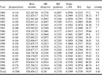
This classification does not differentiate between job-to-job transitions and separations from employment. From the point of view of the pension participant, the nature of how he left his job does not directly effect pension accrual. The longer a worker is at his job, the more valuable his DB plan may be. To agree to a voluntary employment change, a worker with longer tenure and more to lose by changing jobs may receive some extra compensation from his new employer. However, this becomes more likely for workers toward the end of their careers and only if the separation is voluntary. The summary statistics of the sample, by year, are given in Table 1. It seems that the weighted sample gets older, more educated, and sees an increase in real income.
Summary statistics from PSID

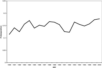
Aggregate employer separation rates for the entire population are given in Figure 1. Looking at the aggregate rates, it seems as if there is no clear trend. However, while aggregate separation rates may have stayed constant, individual rates may have changed. To distinguish individual effects, a series of different logit models are estimated to control for individual and cyclical characteristics.
Aggregate separation rates
Estimated from PSID

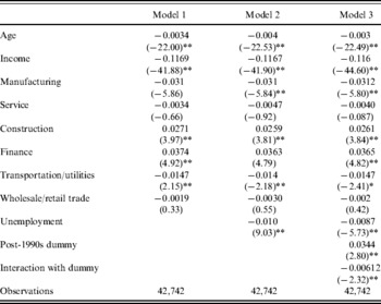
A logit is estimated for model 1 where the dependent variable is separation rates to control for age, income, and industry dummies.Footnote 5 The marginal effects are given in Table 2. Workers that are older and earn more are less likely to change jobs. This is similar to what Polsky (1999) and others have found. Workers in the public administrative and manufacturing industry are less likely to be job changers. Being a worker in the construction or finance industry makes job change relatively more likely.
Marginal effects

Notes: Absolute value of z statistics in parentheses * significant at 5%; ** significant at 1%.
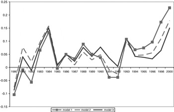
As the sample ages, an increase is seen in real income. Because these factors are inversely related to job changing, they will depress aggregate separation rates. To see what happens when these factors are controlled for, the residuals from model 1 have been obtained and plotted in Figure 2. The separation rates do not seem to follow any trend for the first 11 years, but, starting in the early nineties, the residuals begin to trend upward. This represents changes in turnover controlling for individual effects. It is suggestive that something changed to increase turnover, either a new, more mobile population has joined the sample or the same workers now face different labor market conditions.
Residuals from logit

To see to what extent labor market conditions are driven by the business cycle, model 2 includes the annual unemployment rate. The marginal effect on unemployment is negative and significant. This may seem surprising. However, this is because many of the job changes are employer-to-employer switches. Employer-to-employer separation is more likely in a tighter labor market. This is consistent with the findings of Shimer and labor matching models. The lower the unemployment rate, the more likely a worker is to find another job, and this increases the probability he will leave his current employer. Model 3 includes a dummy variable, which equals one if the year is greater than 1992 and unemployment interacted with this dummy. The 1990s indicator is positive and significant and raises the probability of separation by 3.4%. The negative sign and significance of the marginal effect of unemployment interacted with the 1990s dummy shows that the unemployment rate's effect on turnover was stronger in the 1990s when the labor market was tighter.
The residuals for models 2 and 3 are also included in Figure 2. The residuals for model 2 look a little flatter, but still have an upward trend. Model 3's residuals do not follow any trend. This is suggestive that the increase in turnover in the 1990s can be explained by a stronger cyclicality of job mobility in that period.
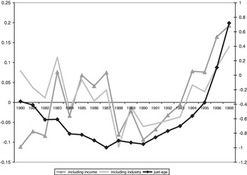
To see which of the individual effects can account for the increased turnover in the 1990s, the residuals for an estimation of just age; age and income; age, income, and industry; and these factors with the unemployment rate are plotted in Figure 3. The aging of the population is the reason why the residuals are increasing. The residuals for the estimation with only age are falling throughout the 1980s, but start increasing sharply in the 1990s. Adding other variables changes the level of the residuals, but the upward trend in the 1990s remains the same. This explains why the aggregate rates have no trend, despite an increase in turnover. The sample has aged, and older workers have become less likely to change jobs. When age is controlled for, there is an increase in turnover rates. The older workers depressed the aggregate trend in the 1990s by being relatively less mobile.
Sensitivity analysis of residuals

The results here suggest that mobility has increased. This finding, while new, is not completely at odds with the existing literature. Farber's 2007 paper, which uses more recent data, reaches a similar conclusion; when you consider turnover by cohort it seems to have increased. Also, the pro-cyclicality of turnover found here suggests that increase in turnover is due to job-to-job transitions, similar to Shimer's findings. Thus, the increase in mobility in the 1990s is most likely from job-to-job switches rather than worker displacement.
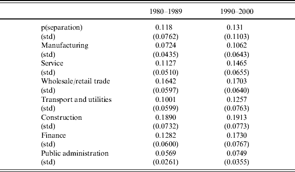
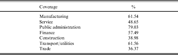
It has been found by Gustman and Steinmeier (1993) and Andrietti and Hildebrand (Reference Andrietti and Hildebrand2001) that jobs that offer pensions also have lower rates of turnover. One way to control for this is to consider individual industries with different turnover and coverage rates. Table 3 gives the predicted rates by industry for the 1980s and 1990s. Public administration, transport and utilities, and the manufacturing industry have the lowest rates of turnover, while construction has one of the highest rates, and each industry sees some increase in turnover. Table 4 gives the pension coverage rates by industry estimated from the 1998 SIPP pension module. Gustman and Steinmeier (1993) and Andrietti and Hildebrand (Reference Andrietti and Hildebrand2001) each found an inverse relationship between pension coverage and the level of turnover. The shift to DC plans has occurred in all industries, and each industry has also seen an increase in turnover.
Turnover rates estimated from PSID

Coverage by industry 1998

Source: SIPP 1998 pension module.
When individual factors are controlled for, there is an upward trend in turnover rates in the 1990s. Higher turnover will mean lower levels of job duration. Lower rates of tenure have significant consequences for the value of the DB pension. Not only does the number of years the worker was with the firm enter directly into the pension formula, but the accrual patterns of DB plans peak at the age of retirement. When a worker leaves a firm early, even if he is fully vested, the value of his pension will be small and frozenFootnote 6 at the value it was at the time of separation. In contrast, if a worker leaves his job and has a 401(k) plan, his pension can continue to accrue. A DC participant can potentially still amass a large amount of pension wealth, even if he experiences significant job turnover. If an employee faces a high probability of job separation throughout his career, the DC scheme may offer significantly higher retirement income.
The shift to DC plans began even before the change in the labor market. The introduction of the 401(k) spurred a large increase in participation in DC plans. By the time the labor market became more variable, DC plans were already quite popular. However, the increase in DC participation continued to increase into the late 1990s, when job separation became more variable. This was also the period in which workers employed by firms that previously had DB plans, as many firms in the manufacturing industry did, became more likely to only have a DC plan. A spike in job-turnover was apparent in the latter half of the 1990s. The findings of Farber suggest this continued to persist into the next decade. Only time will tell if this is permanent, but the shift that coincided with it toward more mobile DC plans suggests that it may be.
3 Life-cycle model
A life-cycle model is constructed for a worker who is offered a DC or DB pension scheme. In period 0, the employee chooses between the plans by taking the option with the larger expected utility. The choice of pension plan is irreversible. Even if a worker changes jobs, he continues to have either the DC or DB plan he chose in the first period. It is as if he finds a job with an identical compensation package. He is also not able to have more than one type of plan. McCarthy (Reference McCarthy2003) allowed workers to have each type of plan simultaneously and found workers prefer the DC plan earlier in their career and start to prefer the DB plan as they age. The purpose of this paper is to obtain a comparison of each plan. In particular, which plan exposes a worker to greater risk, ultimately provides greater levels of utility, and how it influences consumption and asset accumulation. Having the worker have one type of plan throughout his lifetime makes such comparison possible.
It is assumed that the firms offering the pension face no administrative costs; their contributions to the scheme are their only expense. The parameters of each scheme are set so that the expected present discounted value of contributions are equal. In such a case, if firms are risk neutral, they will be indifferent to offering either plan. Firms may be risk neutral, or at least significantly less risk averse than their employees. This may be the case when a firm has many employees and it can hedge the idiosyncratic risk of each employee across other workers. The firm will still face aggregate wage and asset risk, but the risk of individual workers will be averaged out.
The DB plan offers an annuity upon retirement, which is a function of years with the firm and final salary. It is assumed that the DB plan vests immediately.Footnote 7 If the employee leaves the firm after a few years, he still receives a pension, but it is worth less than if he stayed with the job and acquired more tenure. It is assumed that in his next job he starts a new DB plan. If the worker expects to be changing jobs every few years, he will have several DB pensions by the time he retires. Many firms have provisions so that accruals spike around retirement age. For tractability, such provisions are not included in this model, though long tenure at the firm is rewarded and increases with age.
Under the DC schemes, the firm contributes a fraction of the worker's salary to a retirement account each year the worker is employed.Footnote 8 The worker's retirement account follows him throughout his career. As the worker changes jobs, the DC scheme will continue to accrue and future employers will contribute to it.
As shown by Bodie, Marcus, and Merton (Reference Bodie, Marcus, Merton, Bodie, Shoven and Wise1988), even with long-term employment, a DB plan is not without risk. Retirement income in such schemes is a function of wages, so large wage variations cause large variations in retirement income. This model will go further by allowing for a longer time frame. This makes it possible to include transitory and permanent shocks to income. The impact of transitory shocks will have less of an effect on the welfare of the DC participant, because his retirement income is determined by contributions that are a fraction of his earnings each year. So the transitory shocks are effectively averaged out. Transitory shocks will have a larger impact on the DB participant's pension, because it is a function of just one year of wages. Transitory shocks will not be averaged out in this case. Transitory shocks will only penalize the DB plan if they are experienced in the last few years of employment. If they do occur, it can substantially lower the value of a DB plan. However, if these shocks became less likely later in the workers career, they may not pose as large a risk. Transitory income shocks tend to impact on workers whose jobs offer overtime or if compensation is performance based. Depending on the industry and occupation of the worker, the prevalence of these kinds of shocks may or may not vary with age. People employed in government, where DB plans are more prevalent, will experience less transitory shocks than workers in the service industry.
Permanent income shocks will affect the retirement income of each type of pension participant. Unlike transitory shocks, permanent shocks alter the level of income. The value of the DC scheme is a function of annual contributions that are a fraction of income, so permanent shocks cannot be averaged out as transitory shocks can. The final salary at the firm determines the DB pension, so the level of income also determines the DB pension. The fact that the worker faces CRRA utility and incomplete markets and is liquidity constrained means he will have a precautionary saving motive. The presence of this motive means that a positive variance in permanent income will make him want to hold more wealth (Zeldes, Reference Zeldes1984). Large permanent shocks are expected to decrease the welfare of the DB participant more, because a significant fraction of his wealth is the implicit wealth that he will receive in the form of his pension when he retires. This will fluctuate only with wages and tenure. All of the DC participants' wealth is in his stock of assets, which is determined by wages and asset returns. This means that as the worker faces larger permanent wage shocks, all else being equal, he will be more likely to prefer the DC scheme. The fact that the DC participant's retirement wealth varies with something besides his wages means he is in better position to take on more income risk. The extent to which the DC plan dominates the DB plan in the presence of permanent income shocks will vary depending on the portfolio held and how it covaries with wages. If asset returns vary negatively with permanent shocks, the DC participant will be even better diversified and the DC plan will dominate by an even larger degree.
Bodie, Marcus, and Merton (Reference Bodie, Marcus, Merton, Bodie, Shoven and Wise1988) found that asset return variability poses greater risk for a DC participant. The DB benefit is not a function of asset returns; shocks to assets do not directly influence the value of the DB plan. However, it is important to note that if there is an extreme and unexpected movement in asset prices, the probability of the employer defaulting on DB obligations increases. The degree to which longevity risk impacts each type of plan depends on if the participant annuitizes his DC plan. The DB plans are often paid as an annuity, protecting against longevity risk. If the DC participant does not annuitize his assets when he retires, he will have to ensure he does not outlive his assets.
Each type of worker in the model will face stochastic wages, assets, and tenure; but it is assumed that there is zero covariance between the assets and wages. It is assumed that, in each period, there is a positive probability of exogenous job separation. When the worker draws a job change, he will face a larger distribution of wages. An increase in job separation has an impact on the welfare of the DB participant through two channels. It increases the variability of the expected value of the DB plan, which is a function of tenure, and, every time he changes jobs, he exposes himself to larger wage variance. Job changes will also increase the wage variance of the DC participant, but, because of the nature of permanent and transitory shocks, the larger wage variance causes the DC plan to dominate.
Firms
The firms are large and risk neutral. Hustead (Reference Hustead, Olivia and Sylvester1998) found that large firms can finance DB or DC schemes at nearly identical administrative costs. Thus, it is assumed that the only costs the firms face are contributions to the plans. The firm completely finances the DB pension and contributes to the DC participant's pension account.
In a DB scheme, the employer pays the worker an annuity upon retirement and until his death that is a product of the generosity factor, α, and the employee's income during his last year of employment, y ten, and the number of years the worker has been at the firm, Ten

When the firm hires a worker at time, t, it contributes to a fund that will finance future benefit payments. When calculating the expected benefit stream, the firm estimates the expected number of years the worker is expected to be with the firm, his expected salary when he leaves, and how long the worker will be retired – assuming he survives to retirement. The present discounted value of benefits that will be paid each year after retirement, R, until death, T, is

D t is a state variable, in the manner of Hubbard, Skinner, and Zeldes (Reference Hubbard, Skinner and Zeldes1995); that is, 0 if the worker dies and 1 if he continues to be alive. r t is the asset returns in period t, which is the same asset market available to the worker. It is assumed that, once the worker dies, the firm does not pay any more benefits. It is assumed the worker is single, because most DB plans offer survivor benefits.
In the DC plan, the firm contributes a fixed fraction of the employee's income, ρt, into his retirement account when he begins work and in each period until the worker leaves the firm. The expected present discounted value of DC contributions is

where πpsep is the probability of job separation. Assuming the firm is risk neutral, it will be indifferent between offering the DC or the DB pension when:

The firms for a given α set ρt so that condition 1 applies. Condition 1 depends on the assumption that wages follow the same path with either plan. By assuming the wage path and probability of job separation under each plan is identical, condition 1 also assumes the probably of separation is completely exogenous to the model. This is consistent with the empirical evidence that having a DC plan instead of a DB does not increase the likelihood of job separation.
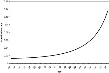
The contribution rate will increase with age. This is because the potential value of a DB plan increases throughout the worker's career as his expected wage and tenure are increasing. The result of this is that DC plans also reward tenure by offering higher contribution rates to long-term employees. The contribution rate by age is plotted in Figure 4. Firms often do offer more generous benefits to their employees with longer tenure. However, the non-discrimination provisions that exist in the US for 401(k) plans limit how much extra compensation can be given to certain employees through a firm-sponsored DC plan.
DC plan contribution rate

Workers with a defined contribution plan
The worker with a DC plan maximizes the following


where θ is the coefficient of relative risk aversion, T is the longest he can live, and R is the retirement date. Y t is period income, which faces two sources of uncertainty, permanent and transitory shocks. His stock of wealth is A t, which accrues at the risky rate r t. He consumes C t, out of his wealth and income Y t each period for t⩽R


for t>R

Transitory income shocks are εc and εnc for job changers and stayers respectively. The permanent component evolves as a random walk with a drift, where G t is the deterministic growth factor that is a function of education, occupation, and industry variables (specific to age t). Permanent income shocks are also state dependent: ηc for changers and ηnc for non-changers. Each period the worker faces a probability, πpsep, that he will become separated from his job and face the ηc and εtc income shocks.
The employer puts a fraction, ρt, of the worker's income into his savings each period the worker is employed with the firm. After the worker retires in period, R, he earns no income and consumes out of his stock of assets. A worker can invest his wealth in an asset that earns a risky rate of return, r t. He also faces longevity risk, represented by the state of whether or not he is alive, D t. If the participant does not annuitize his DC plan, he will face the possibility of outliving his assets. The DB plan is automatically paid as an annuity.
The worker's choice variables are having a DC or DB plan, which is made in period 0, and how much to consume in each period, C t. The state variables are wealth, income, job change, and if he is alive.
Defined contribution plan with an annuity
The DC model also has an annuity variation where the worker annuitizes all of his savings upon retirement. The insurance firms offering annuities are assumed to be risk neutral, face no administrative costs, face perfect markets, and offer fair insurance. The annuity will therefore be a function of the premium,Footnote 9 the probability of survival each year of retirement, and expected asset returns

The annuity-buying worker faces the exact same problem, except now after period R

The worker does not make a consumption choice after retirement. He simply annuitizes all of his wealth at the time of retirement and consumes all of his annuity in each period. This behavior is optimal under the assumption that the worker faces no shocks, other than death, after retirement. If the worker faced some other exogenous shocks, such as a large health care expenditure or the desire to enter a long-term care facility, then there would be some desire to hold wealth or insure against these shocks.
This purpose of the annuitized DC participant variation is to have a benchmark to make DC and DB results comparable. However, while the private annuity market offers DC participants the option to annuitize at least some of their pension, only 7.5% of all DC participants receive their retirement income in the form of an annuity (GAO, 2003). The incidence of annuitization is much higher when a DC plan offers it as an option. However, most DC plans at this time do not offer it, and retirees do not often buy private annuities from independent insurance companies. This is in spite of the fact that fair annuities have been found to be welfare enhancing, Yaari (Reference Yaari1965). This may be due to a number of factors: imperfections in the annuity market, the implicit annuitization of home-ownership, the availability of more liquid instruments, the desire to leave a bequest,Footnote 10 and the annuity from Social Security. All are speculated to reduce the demand for annuities. It is important to consider both versions of the model in comparison to the DB plan. While the annuity option is available, most people choose not to take it and face the longevity risks associated with an unannuitized DC plan.
Workers with a defined benefit plan
The DB participant faces a similar problem except for the nature of his pension


where for t>R


The worker consumes out of his annual income, which follows the same process as the DC participant's income, until retirement. He faces the same asset market as the DC participant, but his employer does not contribute to his savings. Instead, when the DB worker retires, he receives an annuity from each employer based on the number of years he was employed at that firm and his salary when he left that job.
The DB pension incorporates uncertain job tenure in two ways. Each time there is a separation, he faces not only a different wage profile, but starts a new pension plan. There is no distinction if he is separated from his job voluntarily or involuntarily. He will hold a total of f jobs in his lifetime, and job i lasts for ten i years. It is as if the worker becomes separated from his job and immediately finds another with an identical compensation package.
While the features of specific DB plans can vary quite a bit in each firm, this is a fairly typical DB pension according to the Bureau of Labor Statisitcs 2003 survey, ‘Employee benefits in medium and large private establishments’. Just as the 42% of plans offered by private firms, the worker's replacement rate is a fixed percentage per year of service. The worker receives this pension from each of the f jobs he has during his working years. Because the wage path is increasing, the longer a worker is in a job, the greater the value of his pension will be. While some firms (utility, government, some blue collar) have portability provisions that allow accrued wage credits to be transferred to a new job, most firms hold on to benefits until the worker retires. The benefit is frozen at its value at the time of separation, Foster (Reference Foster1994).
To compare the difference in welfare for each scheme, the compensating variation is calculated. Here it is the amount of initial income that would have to be given to the worker to make him indifferent to holding either scheme. If V DC* is the utility maximized level of welfare under each scheme, then the compensating variation, W, is

When W is greater than 0, the worker prefers a DC scheme, and, when it is negative, he prefers the DB plan.
Calibration
The coefficient of relative risk aversion is 3, and the discount rate is one over the mean return on assets. The model is estimated for 61 periods, in the first 39 of which the worker is employed. Retirement is imposed in period 40. It is as if the worker begins his career at age 25 and works until he reaches 65. According to Clark and McDermed (Reference Clark and McDermed1990), the generosity factor, α, actually varies across industries between 0.0094% and 0.024%. Here α is the most popular generosity factor per year of service from the Bureau of Labor Statistics 2003 survey, 0.015. At the beginning of each new job, the contribution rate of the DC plan, ρt, is set so that condition 1 holds. The mortality rates are taken from the Social Security Administration's cohort adjusted life tables, for the male cohort born in 1950. There are no shocks to expected mortality.
The composition of an investor's portfolio can vary across workers depending on education, wealth, and income. Skinner and Samwick (Reference Skinner and Samwick2004) found, looking at the Survey of Consumer Finances, that the share of 401(k) participants invested ‘mostly in stocks’ has steadily increased throughout the nineties. In 1995, 38.22% of respondent's 401(k)s were invested ‘mostly in stocks’, 41.23% were invested ‘split between stocks and bonds’, and 20.55% were invested ‘mostly in bonds’. In the benchmark version of the model, it is assumed that the portfolio is invested 60% in equity and 40% in debt. The return on assets is taken from an estimation by Feldstein and Ranguelova (Reference Feldstein and Ranguelova2001). They estimate a portfolio that is a 60:40 equity–debt mix from the S&P 500 and Salomon Brothers corporate bond index from 1945 to 1995. Assets are assumed to follow a log normal distribution with mean 5.5% and standard deviation of 12.5%. The model is also run for a worker who invests his entire portfolio in equities. He will face an average return of 7% and a standard deviation of 16.6%.
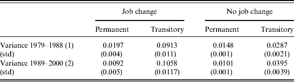
The predictable component of income growth is estimated from PSID using the same sample described in section 2. Wages are estimated as a function of years of education, industry, occupation variables, and age variables that are fitted to a cubic polynomial wage path. The variance is decomposed from the residual of estimated income using the same method as Carroll and Samwick (Reference Carroll and Samwick1997). The variance is estimated separately for workers who changed jobs any time in the period and for those who stayed at the same firm. Separating job changers and stayers is necessary because each job change can result, not only in a transitory shock, but in a permanent one that puts the worker on a different wage path, Topel and Ward (Reference Topel and Ward1992). Similar to Gottschalk and Moffit (Reference Gottschalk and Moffit1994) and Leonardi (Reference Gottschalk and Moffit2003), job changers are classified as anyone who changed jobs at least once during the period. When a worker is classified as a changer, the year in which he changed jobs is included as an indicator in the estimation of transitory and permanent effects. This captures what the permanent and transitory shocks were the year the worker changed jobs. The variance is estimated for two periods, period 1, 1979–1988, and period 2, 1989–2000. The variance for job changers and stayers for both periods is given in Table 5.
Wage variance calibrations estimated from PSID

The variability of transitory income has increased, while permanent income has decreased slightly. As found by Gottschalk and Moffit (Reference Gottschalk and Moffit1994) and Leonardi (Reference Gottschalk and Moffit2003), transitory income shocks are much larger for job changers; implying that most of the variability in transitory income is from job changes. Permanent income variance is also larger for job changers. The sample includes both voluntary and involuntary changes. Permanent wage shocks are more likely to be positive for the voluntary changers, but still pose an element of uncertainty. Transitory income variance may have increased slightly for job stayers because of a shift in the labor force toward more jobs where compensation is outcome based. For example, service industry jobs are more likely to base pay on commission.
The probability of job separation is also estimated from PSID. It is found by estimating the predicted turnover rates, using model 2's specification, for the given characteristics at the beginning of each period. Separation rates for the entire population and for the manufacturing, service, whole sale and retail trade, transport and utilities, construction, finance, and public administration industry are given in Table 3. The probability of job separation for the total population increased by about 2%. Not only has the probability of separation increased, but the standard error has increased as well. This is suggestive of even more uncertain job prospects. Separation rates increased the most in the manufacturing and finance industry. Industries with high turnover rates, construction and trade, experienced an increase, though the magnitude was not very large. Manufacturing has one of the lowest separation rates, but experienced about a 3.4% increase.
4 Results
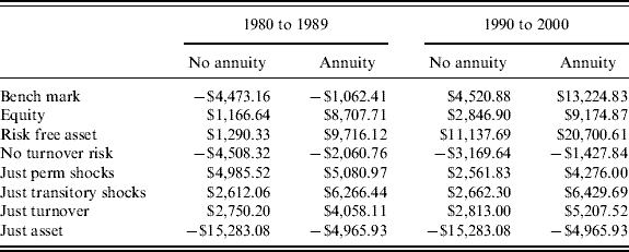
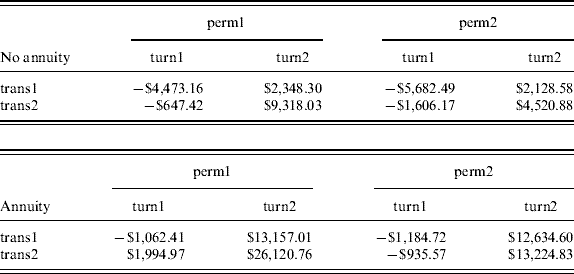
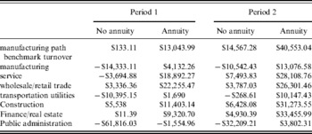
The model is solved for the level of utility each type of plan provides. If one plan offers lower welfare than another, the amount of money a participant would need to be given in the first period to be indifferent between the two options, the compensating variation, is calculated. The compensating variation is given for the first period, 1980–1988, and second period, 1989–2000 in Table 6. In the first period in the benchmark version of the model, the worker prefers the DB scheme to the DC. The DB participant would need to pay about $4,473Footnote 11 to be indifferent to a DC plan. When transitory wage and turnover variability increased in period 2, his preferences changed. The DB participant would need to be given about $4,520 to be indifferent to having a DC plan. The DC plan has become the dominant choice of pension plan.
Compensating variation

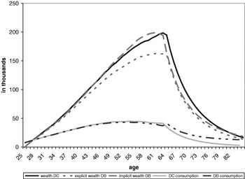
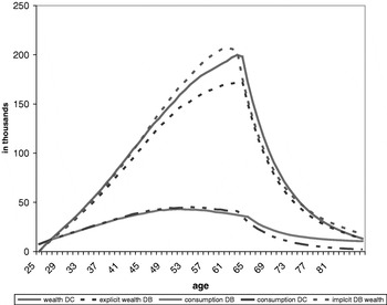
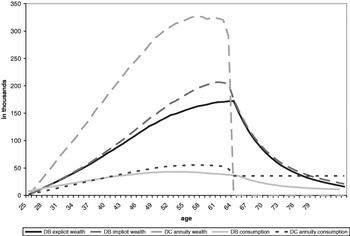
The simulated consumption and wealth paths for periods 1 and 2 are given in Figures 5 and 6. In each period, the DC participant has more explicit wealth and slightly higher consumption during his working years, and the DB plan provides more consumption during retirement. The DC participant has more explicit wealth, because he has a higher saving rate and the employer is directly contributing to the worker's assets. The accumulated DB pension is not included in wealth, because it is given as income after retirement. This is often the reason given why 401(k) participants are found to have more wealth than DB participants. In the simulated wealth paths here, implicit DB wealth includes the accumulated DB credits. Throughout most of his life, the DC participant's wealth is about equal to the DB participant's implicit wealth. In the first period during his middle age, he will have more implicit DB wealth, but, in the years just before retirement, his DC wealth increases and is higher than all DB wealth. In the second period under both regimes, he saves more, because he faces more variable wages. His implicit DB wealth is higher, starting at age 46 and through retirement, because he is more exposed to wage shocks than the DC participant. The precautionary motive will make him want to hold more wealth.
Average wealth path (period 1)

Average wealth and consumption path (period 2)

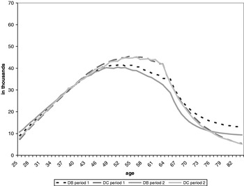
In Figure 7, the consumption paths under each scheme for both periods are plotted. Consumption is hump-shaped, because, in the beginning of the workers life, he has lower income and is liquidity constrained. His consumption declines after retirement, because the probability of dying increases. There is a slight kink in the consumption path at the time of retirement, because, after retirement, the worker is solving a different problem where he no longer faces wage and turnover shocks. The consumption path for the DC participant is slightly lower in period 2, because the worker faces greater wage risk. Consumption decreases for the DB participant in period 2 by a much larger degree. This is so for two reasons. The larger turnover rate lowers the expected value of the DB pension, so the worker will want to acquire more wealth to increase his post retirement income. Also, the worker has a precautionary motive, and the increase in turnover and wage variability will make the DB participant want to depress consumption in order to hold more assets. The DB holder is more sensitive to turnover and wage shocks, so the increase in these variables will not have as large an impact on the DC participant. He does not modify his consumption to the same degree.
Average consumption paths

First shown by Yaari (Reference Yaari1965) and estimated numerically by Brown (Reference Brown2001), full and fair annuitization is always welfare enhancing. The compensating variation is always larger for the DC plan with an annuity. The difference in welfare between the annuitized and unannuitized DC plan may be partially driven by the lack of social security in the model. Without an annuity, the worker's income goes to 0 after retirement. Including social security in the model is not expected to have a large impact on the welfare of the DC with annuity or DB participant. They are each already receiving some post retirement income, but it may increase the desirability of the unannuitized DC plan. Even with full annuitization under the DC plan, the worker prefers the DB plan in period 1, though by a smaller degree by just $1,062. In the second period, he now would need to be compensated $13,224. This is more than his initial income.
In Figure 8, the wealth and consumption paths for the DC participant who has an annuity is plotted. His consumption profile is flatter than the DB holders, and consumption is higher after retirement. The worker's consumption stream is also much flatter than it would be if he did not annuitize. This is because he now faces no uncertainty after retirement. It also is why annuities are welfare enhancing.
Average consumption and wealth path with an annuity

Sensitivity analysis
The change in preference in the benchmark model is driven by the fact that three of the parameters values have changed: the probability of job separation and transitory and permanent wage variance. Transitory income shocks have increased by nearly 20% for job changers and have almost doubled for job stayers. The probability of turnover increased by almost 2%. The increase in each of these factors has made the DB scheme less desirable. Permanent shocks have actually decreased which will work in the opposite direction, increasing DB welfare relative to DC. The magnitude of the decrease in permanent shocks is rather small. It increased by just 0.007 for changers and by 0.005 for stayers. The increases in turnover and transitory variance dominate the decrease in permanent shock, causing preferences to change in the second period.
Table 7 gives the compensating variations for all the permutations of each period's calibrations. The increase in turnover drives a large part of the result. When the worker faces period 2's wage shocks and period 1's turnover shocks, he will always revert to his period 1 choice, though the DC plan dominates by a smaller degree. When he faces period 2's turnover shocks and period 1's wage shocks, he will prefer the DC scheme. Again, this is because higher turnover increases the variability of the expected value of the DB plan relative to the DC plan and the worker faces more variable wages. These factors decrease the desirability of DB plans. When the worker faces only turnover risk, but no asset or wage risk, he will prefer the DC plan, though the difference between each period is much smaller because the extra wage uncertainty is not present.
Sensitivity analysis

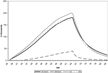
When the worker faces only wage and asset, but no turnover risk, he will always prefer the DB plan. This is because he faces a less variable income path and is guaranteed a replacement rate of 58.5%. The average wealth path for period 2's wage parameters and a zero probability of job separation is given in Figure 9. The DB participant now holds much less explicit wealth than the DC participant. He will still want to hold some wealth to protect him from wage shocks, but wealth is always at a much lower level than it was when he faced turnover risk. This is because the wage shocks he faces are now smaller, because he is not exposed to the job change wage distribution. He is also now guaranteed a 58.5% replacement rate upon retirement, so he does not have to accumulate as many assets to finance his retirement consumption. The DC participant also lowers his wealth holdings when he faces no turnover risk. This is because his wage variability has also decreased.
Average wealth path without turnover risk (period 2)

As transitory shocks increase, the DC scheme becomes more desirable. If period 1 transitory shocks are used in period 2, he will still prefer the DC plan, but by a smaller degree. The DC scheme becomes welfare enhancing relative to the DB plan as transitory variance increases. When the worker faces only transitory shocks, the DC plan dominates, and the magnitude of this increases with the size of the transitory shock. This is consistent with the findings of Bodie, Marcus, and Merton (Reference Bodie, Marcus, Merton, Bodie, Shoven and Wise1988), who show that, when faced with transitory wage shocks as the only source of risk, the worker will always prefer the DC plan. This is because transitory shocks are averaged across years in a DC scheme, but in a DB scheme the pension is based only on the final draw of income. The DB participant faces greater exposure to transitory wage risk.
Larger permanent income shocks increase the welfare gains of having a DC plan. When period 2's parameters are run with period 1's permanent shocks, the worker prefers the DC by a larger degree than he did with all period 2 parameters. This is because period 1's permanent wage shocks are a little bigger than period 2. This is because the DB participant is more vulnerable to permanent wage shocks than the DC participant. The DB holder's retirement wealth is a function primarily of his final wage, while the DC participant's retirement wealth is also a function of asset returns. When faced with permanent wage shocks, the DB worker will want to decrease consumption by a larger degree to account for this. With no other form of uncertainty but permanent shocks, the DC plan is more desirable.
When the worker's portfolio is invested entirely in equity, he is more likely to prefer the DC plan. While he faces larger asset variance, he also earns a higher expected return. The equity premium puzzle is present here, in that the worker prefers higher expected returns even with greater variance. The DC plan also becomes more desirable when the worker faces no asset risk but wage risk. This is the case to an even larger degree in period 2, when turnover and transitory shocks are larger. This is consistent with the findings of Bodie, Marcus, and Merton, who proved that, when faced with only wage risk, a DC scheme will always be the dominant choice. When the worker only faces asset risk and certain wage and tenure, he will prefer the DB plan, which is also consistent with the Bodie, Marcus, and Merton result.
By industry
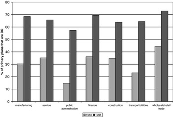
The degree of pension coverage varies across different industries. This can be seen in Table 4. However, the shift to DC plans has occurred within each industry. This can be seen in Figure 10. It shows the percentage of workers with a pension plan who claim a DC scheme as their primary plan in 1983 and 1998. DC participation has overtaken DB in all of the industries, though to varying degrees.
% of primary plans that are DC estimated from SIPP 1983 and 1998

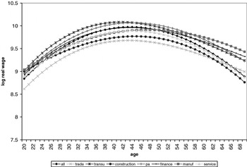
The change in preferences is driven by an increase in the probability of job separation and transitory wage variance. Another factor that drives the result is the shape of the predictable income path. The predicted wage paths for each industry are given in Figure 11. The trade, public administration, and manufacturing industries each face flatter wage paths, while construction's is steeper and lower than the other industries. The service and transportation/utilities each have wage paths that are slightly flatter.
Wage paths for industries estimated from PSID

To see how the wage path affects preferences, the benchmark parameters are run with the wage path of the manufacturing industry. This is one of the flattest of all the wage paths. When the model is run with the manufacturing wage path, the worker will always prefer the DC scheme. This is because the flatter wage path will lead to greater asset accumulation. The DC worker will experience the benefits of this more, because the firm is contributing a fraction of his wage to his wealth in each period. The implicit DB wealth will also be larger because the wage path is flatter, but, as wage shocks increase, the DC scheme becomes even more welfare enhancing. The worker has even more wealth to buffer him against wage shocks. Cocco and Lopes (Reference Cocco and Lopes2004) also found that a DB plan was more desirable for workers with steeper wage paths.
Table 8 also includes the compensating variation for the model run with the wage paths and turnover rates for seven different industries: manufacturing, service, public administration, finance, construction, wholesale/retail trade, and transport and utilities. Turnover rates in the manufacturing industry are quite a bit lower than the rate for the entire population, 7.2%, in period 1, and 10.6% in period 2. In this scenario, the DB plan now dominates the DC plan without an annuity in period 2. However, the annuitized DC plan is now always the welfare-enhancing choice. The desirability of the annuitized DC scheme may seem surprising, because the manufacturing industry has traditionally been associated with high levels of DB participation. However, this industry faced a large increase in turnover during the 1990s. That the annuitized DC plan now dominates may explain why DC participation has overtaken DB. In the manufacturing industry in 1983, about 70% of participants reported a DB plan and 30% reported a DC as their primary plan. This nearly reversed by 1998. The flatter profile and higher separation rates have made the DC plan even more desirable in the second period. This may explain why the service industry has also seen an increase in DC coverage. The model predicts that the service industry worker will now prefer the annuitized DC plan and prefer the unannuitized DC plan by a lesser degree in period 1. This could be one reason why the DC plan was relatively popular in the service industry in 1983 and so dominant in 1998. In period 2, the DC plan is even more welfare enhancing.
Compensating variation by industry

Public administration has one of the highest rates of coverage and lowest rates of turnover. It also has experienced one of the largest increases in DC coverage. The model predicts that the DB plan will be the most desirable in this industry, though, in period 2, the DC plan with an annuity becomes the dominant choice and the degree to which the DB plan dominates falls by more than 90%. Public administration's separation rate is still relatively lower than other industries, about 7.5%, but the increase in turnover has made an annuitized DC plan the dominant choice in period 2. Transport and utilities has seen one of the largest increases in DC coverage and also has a high rate of pension coverage. It has also seen more than a 2.5% increase in turnover. The model predicts that this increase in turnover has made the annuitized DC plan the dominant choice in period 2. The worker still prefers the DB plan to the unannuitized DC plan in period 2, though to a much smaller degree; his compensating variation is just 1.8% of initial income.
Industries with higher rates of turnover: construction, finance, and trade, are also the ones where the DC plan dominates by the greatest degree. Trade and construction have high rates of job separation, though turnover has not increased by very much, less than 1%. The model predicts the DC plan to dominate in both periods. It can be seen in Figure 10 that DC plans were already relatively popular in these industries in 1983, and, by 1998, the trade industry has the highest rate of DC coverage. The finance industry has seen one of the largest increases in turnover. In period 1, the participant is nearly indifferent to the DB plan and the unannuitized DC plan, and DC dominates in both cases in period 2. Finance has one of the highest rates of DC coverage in 1998, though the increase in DC coverage is smaller than it is in other industries. This is because DC plans were already relatively prevalent in the finance industry in 1983. The model predicts DC plans to be popular in high turnover industries in the 1980s. However, while DC plans were more popular than they were in other industries, DB participation was still larger. This is because, in the early 1980s, 401(k)s were still new, and it took some time for firms to adopt them. The model would predict that the high turnover industries would be the quickest to adopt them; these industries would now have the highest levels of DC coverage. This does seem to be the case in the construction, finance, and trade industries.
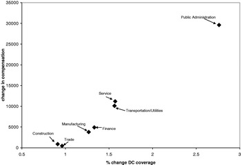
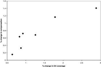
Figure 12 is a scatter plot of the change in compensating variation between period 1 and 2 on the y-axis and the percentage change in DC participation between 1983 and 1998 on the x-axis for the model without an annuity. The change in compensating variation across periods is positively correlated with the growth of DC participation across industries; there is a clear upward trend. Figure 13 is a scatter plot of the percentage change in compensation for an annuitized pension on the y-axis and the percentage increase in DC coverage on the x-axis. For the annuity holder there is also an upward trend. The positive correlation between changes in welfare and changes in DC coverage shows that the model's predictions are consistent with actual industry trends. DC coverage has increased in all industries, but the model predicts this has been the case to the largest degree in industries for which the DC plan offered the greatest increase in welfare.
Scatter plot of change in compensating variation and change in DC participation for by industry with out annuity

Scatter plot of change in compensating variation and change in DC participation for by industry with annuity

5 Conclusion
This paper measures the relative risks of DC and DB pension plans in a life-cycle model. There has been a remarkable increase in the number of individuals with private pension accounts for which they are responsible for investing and solely bearing the asset risk. This has raised concerns about the level and variability of retirement income that private accounts can provide. That DC plans can generate higher retirement income has been shown by Skinner and Samwick (Reference Skinner and Samwick2004). It has also been shown by Bodie, Marcus, and Merton (Reference Bodie, Marcus, Merton, Bodie, Shoven and Wise1988) and McCarthy (Reference McCarthy2003) that, with enough wage risk, DC plans can dominate DB plans. However, such estimates do not capture all the elements of risk in having a DB plan. Including only wage and asset risk underestimates the retirement income that DB plans provide. Because tenure is part of the DB plan function, and lifetime employment is often not guaranteed, it is necessary to treat tenure as a random variable and consider how it has evolved. It is found, when controlling for demographic changes and extending PSID to 2000, that job turnover rates have increased. When calibrations for job turnover and wage variance are estimated from the 1980s and 1990s and used in the life-cycle model, where the worker chooses between a DC and DB plan, the DC plan becomes the dominant choice in the latter period, 1989–2000.
The boom of the 1990s increased job mobility and wage variance. The increase in each of these factors, particularly turnover, has decreased the desirability of DB plans. The model predicts that younger cohorts are more likely to have a DC plan as their primary pension, which has been the case. The model predicts that industries with higher turnover rates will have experienced an increased prevalence of DC plans. This can also be seen in the data. DC coverage has increased in all industries, but generally this has been true to a greater extent in industries which experienced larger increases in turnover.
The model has some limitations. In particular, it does not include Social Security, which is expected to increase the relative desirability of the unannuitized DC plan. It also does not include the special tax treatment of DC contributions. Including taxes in the model may further increase the savings rates of DC participants. Also, while the worker can consume out of his 401(k) plan, there is some penalty for doing so. Including such a penalty may decrease the desirability of DC plans. The model can also be extended to allow workers to hold two types of plans at once.
A life-cycle model assumes that the workers fully understand their job and investment prospects as well as how the benefits are calculated. Particularly for DB plans, the benefit formula is often not transparent, and it has been shown by Gustman and Steinmeier (Reference Gustman and Steinmeier1999) that workers may not even be fully aware of the type of plan they have. The model could also be extended to include a bequest motive and survivor benefits.
The results suggest that cash balance plans have been under utilized. Cash balance plans allow a worker to, upon separation from his job, transfer his wage credits into a private account that can continue to accrue. Such a scheme incorporates some of the DB plan's desirable features, an annuity and replacement rate, without turnover risk. Many firms converted to cash balance plans in the late nineties, but such plans are extremely unpopular with older, more vocal workers who faced ungenerous grandfathering provisions. As long as higher rates of turnover and income variance can decrease the welfare of DB pension participants relative to DC, there is scope to design plans that can combine the welfare-improving properties of each of these schemes.