I. INTRODUCTION
In many engineering components made of various materials (including ceramics, metals, and glasses), residual stresses are introduced by thermal mismatch or mechanical/thermal processing during their manufacturing, welding/joining, and sintering operations. Reference Arsenault and Taya1,Reference Dong and Brust2 For example, heat from welding may cause localized expansion, which is taken up during welding by either the molten metal or the placement of parts being welded. When the finished weldment cools, some areas cool and contract more than others, leaving residual stresses. Another example occurs during semiconductor fabrication and microsystem fabrication when thin film materials with different thermal and crystalline properties are deposited sequentially under different process conditions. The stress variation through a stack of thin film materials can be very complex and can vary between compressive and tensile stresses from layer to layer.
Residual stress is that which remains in a body that is stationary and at equilibrium with its surroundings. It can be very detrimental to the performance of a material or the life of a component. Alternatively, beneficial residual stresses can be introduced deliberately. For instance, for a structural component undergoing an applied stress, the compressive residual stress enhances the resistance to crack propagation, whereas tensile residual stress reduces the resistance. For semiconductor devices, residual stresses may decrease their service life sharply, however, with the use of internal stresses, it is possible to considerably increase the mobility of charge carriers and thus the charge speed of the device can be increased markedly. Reference Golovin3 Residual stresses are more difficult to predict than the in-service stresses on which they superimpose. For this reason, it is important to have reliable methods for the measurement of these stresses and to understand the level of information they can provide.
The conventional methods for measuring residual stresses can be divided into two groups: mechanical stress-relaxation methods and physical-parameter analysis methods. Mechanical stress-relaxation methods, including hole-drilling and saw-cutting techniques, are generally used to measure residual stress quantitatively without any reference sample. However, the destructive nature of these methods limits the wide application of these techniques in industry. Whereas, physical-parameter analysis methods, including ultrasonic wave, Reference Hu, He and Chen4 magnetic Barkhausen noise, Reference Gauthier, Krause and Atherton5 x-ray, Reference Gou, Zhang, Xu, Sun and Yang6 and neutron diffraction, can measure residual stresses indirectly and nondestructively, and some methods have been partially used in industrial fields. However, one limitation of this group of methods is that it is difficult to separate intrinsic microstructural effects on the physical parameters from the effects of a residual stress, and hence the methods require the preparation of stress-free reference sample for comparison purpose. Additionally, the physical methods cannot be directly applied to amorphous/glass materials, such as a large-scale glass display panel and a shot-peening bulk metallic glass, which do not have a long-range ordered atomic structure.
Another technique for the measurement of residual stress is the instrumented indentation, it has rapidly emerged as a powerful tool for exploring mechanical behavior of a small volume in the past two decades. The instrumented indentation has been used to measure the mechanical properties of materials, such as the hardness, H, Reference Doerner and Nix7,Reference Oliver and Pharr8 elastic modulus, E, strain-hardening exponent, n, Reference Dao, Chollacoop, Van Vliet, Venkatesh and Suresh9,Reference Jang, Choi, Lee, Lee, Kwon, Gao and Kania10 yield strength, σY, Reference Field and Swain11,Reference Swain12 and small-scale mechanical behavior (e.g., indentation size effect Reference Bushby and Dunstan13,Reference Zhu, Bushby and Dunstan14 ). During indentation, a rigid indenter is penetrated normally into a homogeneous solid while the indentation load, F, and depth, h, are continuously recorded during one complete cycle of loading and unloading. Because the load–depth curves of indentation contain abundant information about material properties, indentation can be used to evaluate material properties. General observations reveal that tensile stress tends to stretch out the load–depth curves to smaller forces, while compressive stress compresses the curves to larger forces. Reference Suresh and Giannakopoulos15 Thus, indentation can also be used to evaluate the residual stress.
Several methodologies have been introduced to estimate residual stress using instrumented indentation. The earliest effort was to examine the relationship between hardness and residual stress using indentation techniques. The results suggested that hardness measurement may be used to characterize residual stress in materials. Reference Suresh and Giannakopoulos15,Reference Cheng and Cheng16 However, the alteration in hardness by the residual stress was less than 10% of its unstressed value, and the effects of compressive stress are often not as large as tensile stress. Reference Tsui, Oliver and Pharr17 More recently, many studies have been undertaken to develop new ways for measuring residual stress using instrumented indentation, because this nondestructive/mechanical technique can overcome the limitations of conventional methods including both the destructive/mechanical and nondestructive/physical methods. A number of useful reviews on instrumented indentation are available. Reference Fischer-Cripps18–Reference Oliver and Pharr21 Although applying instrumented indentation as a simple nondestructive/mechanical test for that purpose has clear advantages, there are some issues remaining unresolved.
The most important problem in the residual stress measurement is that the current indentation method cannot be applied to a material showing a strong dependence of the residual stress on its direction while the indenters basically give an average response of the surface residual stress. Note that residual stress states determined by current instrumented indentation techniques are mostly restricted to equi-biaxial or uniaxial stress. Reference Chen, Yan and Karlsson22 Although some models Reference Lee and Kwon23 provide general residual stress solutions, the stress ratio should be known independently. Some efforts have been made by Lee et al. Reference Lee, Takashima, Higo and Kwon24 to obtain the ratio of two principal stresses by measuring the pile-up height ratio, this approach is admirable, but the direct relation between residual stress and pile-up displacement is not given. More recently, some attempts have been made using an asymmetric Knoop indenter, Reference Kwon, Lee, Han, Lee, Lee, Choi and Kim25 but the method has not been fully established yet.
In this work, a novel method is put forward for solving the problems aforementioned during the measurement of residual stresses under the condition of both uniaxial and biaxial stress. Finite element simulation is adopted to study the development of pile-up during indentation with a rigid sphere under the condition of residual stress. It is found that the direction and amplitude of the maximum residual stress can be determined by measuring the maximum pile-up displacement around an indentation after unloading. The relation between the pile-up displacement after unloading and the biaxial surface residual stress is studied and obtained quantitatively.
II. GENERAL DESCRIPTION
For measuring material properties by load and depth sensing indentation methods, it is essential that the contact geometry is established precisely since analysis procedures used for determining properties like the hardness, H, and elastic modulus, E, rely heavily on an accurate measurement of the contact area. Reference Oliver and Pharr8 However, the measurement of the contact area from the load–depth data is not a straightforward process, as it depends on the pile-up or sink-in of material around the contact impression. Bolshakov and Pharr Reference Bolshakov and Pharr26 examined the significance of pile-up for rigid conical indenters and found that if pile-up is neglected, the true contact area can be underestimated by as much as 60%, leading to similar errors in calculated material properties. Thus, a complete understanding indentation of pile-up and sink-in is crucial to making accurate property measurements.
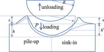
For spherical indenters, the pile-up and sink-in geometry may change significantly during indentation by virtue of the transition from purely elastic deformation at small depths to plastically dominated behavior at large depths. The contact geometry for spherical indentation is illustrated in Fig. 1, which shows a rigid sphere of radius R driven into a material by a force P to a penetration depth h. The right-hand side of the figure shows the behavior when material sinks-in and the left-hand side shows pile-up.
Spherical indentation contact geometry.

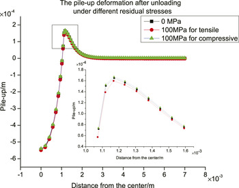
When the pressure on the indenter is removed, the contact impression will partially recover due to elastic processes. The indentation depth h will recover to h ′, the pile-up will increase, and the sink-in will convert to pile-up after unloading for some material. The permanent deformation was rarely considered in previous literature. And the pile-up displacements after unloading will change significantly with different residual stresses, as shown in Fig. 2. The load on an indenter is 1500N and the yield stress of a material is 400 MPa. Figure 2 describes indentation responses under three different conditions: 100 MPa compressive stress, unstressed, and 100 MPa tensile stress. The indentation depth is 539.92, 544.47, and 548.98 μm, respectively.
Pile-up after unloading under different residual stresses.

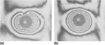
Underwood Reference Underwood27 introduced an optical-interference method to observe the permanent surface deformation around an indentation in steel. From his experimental results, it is observed that different residual stresses correspond to different pile-ups around an indentation after unloading under the condition of uniaxial residual stress. This implies that the direction and amplitude of residual stress are dependent on the deformation around an indentation after unloading. However, it is difficult to deduce the theoretical relationship between them because of the complexity. Hence, the finite element method is used here to study and establish such relationship.
III. INFLUENCE OF MATERIAL PARAMETERS
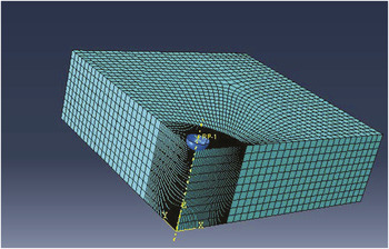
Simulation of the spherical indentation process was performed using the Abaqus® finite element software (Hibbitt, Karlsson & Sorensen, Inc., Rhode Island). As shown in Fig. 3, a 1/4 model for finite element mesh around an indentation was used. Figure 3 shows a sketch map of the element mesh, the indenter was modeled as a rigid sphere of radius R = 2.5 mm, and to make the results more accurate, the bulk specimen with a size of 30 mm × 30 mm ×10 mm was discretized into 3260,000 elements, the mesh was local refined around the indentation. Roller boundary conditions were applied at the bottom surface by enforcing no displacements in the z direction and free movement in the x and y directions. Symmetry boundary conditions were applied and a free boundary condition was applied on the other surface of the specimen except the region of the top surface contacting with the indenter. In most computations, a friction coefficient was used to describe the interface between the indenter and the specimen, the influences of friction were examined using: m = 0, 0.05, 0.1, and 0.15.
Finite element mesh around the indentation.

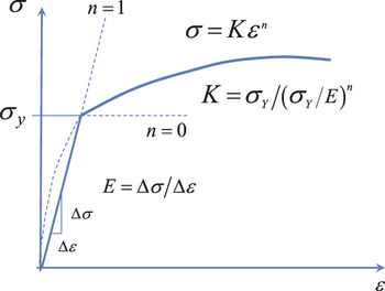
Figure 4 shows the assumed elastic–plastic constitutive law. Linear elastic behavior with Young's modulus E and Poisson's ratio μ = 0.3333 was assumed up to the yield stress σY. Thereafter, the behavior was modeled as elastic–plastic with power-law hardening of the normal form σ = Kε
n
. To assure continuity at the yield point, the strength coefficient, K, was related to other material parameters through
 $K = {{\sigma _{\rm{Y}} } \mathord{\left/ {\vphantom {{\sigma _{\rm{Y}} } {\left( {{{\sigma _{\rm{Y}} } \mathord{\left/ {\vphantom {{\sigma _{\rm{Y}} } E}} \right. \kern-\nulldelimiterspace} E}} \right)}}} \right. \kern-\nulldelimiterspace} {\left( {{{\sigma _{\rm{Y}} } \mathord{\left/ {\vphantom {{\sigma _{\rm{Y}} } E}} \right. \kern-\nulldelimiterspace} E}} \right)}}^n$
. A rate-independent model based on Mises flow theory with isotropic hardening was used in the computation.
The elastic–plastic constitutive law.

A. Influence of hardening exponent on pile-up
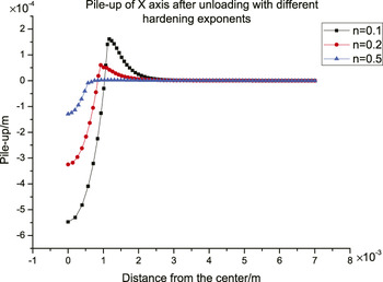
Assuming that the hardening exponent n varies from 0.1 to 0.5, which contain most of the materials, the load on the indenter is 1500N, and the residual tensile stress is 100 MPa, one can obtain the plots of the pile-up after unloading in x axis with different hardening exponents, as shown in Fig. 5. When the hardening exponent n is equal to 0.1, 0.2, and 0.5, the corresponding depth of indentation is 548.23, 325.43, and 129.16 μm, respectively.
Pile-up of x axis after unloading with different hardening exponents.

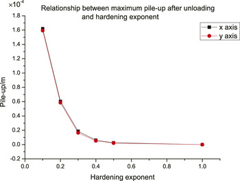
Taking the maximum pile-up data from the simulations, the relationship between the maximum pile-up and the hardening exponent can be obtained and is shown in Fig. 6. It can be seen from Figs. 5 and 6 that the maximum pile up after unloading around the indentation depends strongly on the hardening exponent and decreases with the increase of hardening exponent.
Relation between the maximum pile-up after unloading and hardening exponent.

B. Influence of E/σY
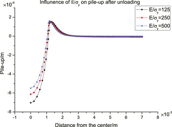
The evolution of pile-up during the indentation testing is strongly dependent on the relative amounts of elastic and plastic deformation that is characterized by the ratio of the elastic modulus to yield stress, E/σY. This parameter physically represents the reciprocal of the elastic strain at yielding which can be used as a measure of the amount of deformation accommodated elastically during indentation. In the limit of E/σY = 0, the contact is strictly elastic as predicted by Hertzian contact mechanics. At the other extreme, the limit E/σY = ∞ corresponds to rigid-plastic deformation, for which there is extensive pile-up of material around the hardness impression.
Assuming that the residual tensile stress in material is 100 MPa, the simulated responses with different material parameters E/σY are shown in Fig. 7. As the parameter E/σY increases, the maximum pile-up after unloading increases.
Influence of E/σY on pile-up after unloading (n = 0.1).

C. Influence of friction
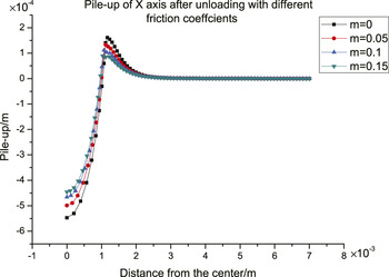
Assuming n = 0.1, the load on the indenter is 1500N, and the residual tensile stress is 100 MPa, the friction coefficient m is set to be 0, 0.05, 0.1, and 0.15, respectively, we obtain the relationship between the pile-up of x axis and the friction coefficient, as shown in Fig. 8.
Pile-ups of x axis after unloading with different friction coefficients.

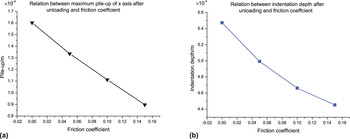
Taking the maximum pile-up from the data in Fig. 8, one can obtain the linear relation between the maximum pile-up and the friction coefficient, as shown in Fig. 9(a), and the maximum pile-up after unloading decreases with the increase of friction coefficient, so does the indentation depth in Fig. 9(b).
(a) Plot of maximum pile-up displacement of x axis after unloading versus friction coefficient and (b) plot of indentation depth after unloading versus friction coefficient.

IV. SIMULATION AND DISCUSSION
A. The relationship between uniaxial residual stress and the pile-up after unloading
Assuming that the residual stress is applied in the x direction of the specimen and change from tensile to compressive in the range of −350 to 350 MPa, in which “−” means compressive stress and “+” means tensile stress. The yield stress σY is 400 MPa. The out-of-plane displacements around the indentation after unloading can be calculated by the finite element simulation. To obtain meaningful pile-ups for estimating residual stress, an appropriate load should be applied on the indenter. For the material mentioned above, the load is set to be 1500N. In this case, the unstressed pile-up is 164.6 μm and can be easily recognized by an optical measurement system. To compare with Underwood's experimental results, the calculated out-of-plane displacements are shown in the forms of interference fringes.
If a laser microscope for measuring out-of-plane displacement is used as Underwood Reference Underwood27 did, the intensity of the interference fringes Reference He, Tay and Shang28 can be expressed as:
 $$I = A{\cos ^2}{\delta \over 2}\quad ,$$
where I is the intensity of the interference fringes, δ is the phase difference, and A is a constant.
If the observation direction and the laser illumination direction are the same, the relation between displacement and phase difference can be written as:
 $$d = {{\delta \lambda } \over {4\pi }}\quad ,$$
where d is the pile-up displacement and λ is the wave length of the laser.
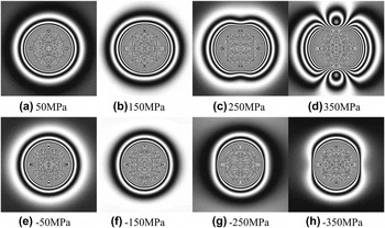
The interference patterns with simulation method for different residual stresses are shown in Fig. 10. The wave length is set to be λ = 0.6328 mm. Different wave lengths can lead to different densities of fringe patterns.
Simulated interference patterns of pile-up after unloading under different uniaxial residual stresses from −350 to 350 MPa. (a) 50 MPa, (b) 150 MPa, (c) 250 MPa, (d) 350 MPa, (e) −50 MPa, (f) −150 MPa, (g) −250 MPa and (h) −350 MPa.

The distribution of pile-up around the indentation, as shown in Fig. 10, is a two-lobed pattern as the applied tensile residual stress increased. This shape feature is quite similar to the experimental observation of Underwood, Reference Underwood27 as shown in Fig. 11.
Underwood's interference fringe photos of indentations (a) uniaxial tensile residual stress and (b) uniaxial compressive residual stress.

On further analysis of the fringe shape and the out-of-plane displacements obtained by simulation, we found that the direction of the tensile stress coincides with the prominent direction of arc, and the maximum pile-up along the radial direction appears in x axis, which is the tensile direction. On the contrary, the fringe shape of the pile-up around the indentation with compressive residual stress is nearly an ellipse, the minor axis coincides with the direction of the compressive stress. The maximum pile-up along the radial direction appears in y axis. Therefore, by using this method, the direction of the uniaxial residual tensile or compressive stress can be easily determined.
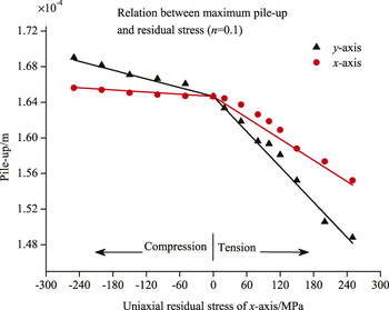
The curves of pile-up displacements along x and y axes after unloading versus residual stresses are shown in Fig. 12. The data imply a bilinear relation between the maximum pile-up and residual stress after unloading, for both x axis and y axes. For compressive residual stress, the maximum pile-up of y axis is larger than that of x axis. Contrarily, for tensile residual stress, the maximum pile-up of x axis is larger than that of y axis.
Relations between residual stress and maximum pile-up of x and y axes after unloading: uniaxial residual stress along x-axis.

A number of simulations with different parameters had been done to study the pile-up under different uniaxial residual stresses. After careful studies and analysis, the relationship between uniaxial residual stress and the maximum pile-up after unloading can be set as follows:
 $${{{s_x}} \over {{s_0}}} = - {C_{11}}{{{\sigma _{{\rm{res}}}}} \over {{\sigma _{\rm{Y}}}}} + 1\quad ,$$
where s x is the maximum pile-up along x axis, s 0 is the maximum pile-up without residual stress, σres is the uniaxial residual stress along x axis, and σY is the yield stress. Friction is not considered here. If the residual stress is compressive, C 11 = 0.009232, and if the residual stress is tensile, C 11 = 0.09168. The value of the uniaxial residual stress can be calculated from Eq. (3).
B. The relationship between biaxial residual stress and pile-up after unloading
Assuming that the residual stress of x axis is in tensile state and the value is 100 MPa, the residual stress of the y axis changes from tensile to compressive and varies from −250 to 250 MPa. The out-of-plane displacements around the indentation after unloading under the condition of biaxial residual stress can be calculated by the simulation and the corresponding full-field interference patterns can also be formed by using Eq. (2).
If the tensile stress along x axis is 100 MPa and the tensile stress along y axis is also 100 MPa, it is the equi-biaxial residual stress. The interference patterns are a series of circles. When the stress of y axis is larger than that of x axis, the interference patterns are a series of vertical ellipses and the maximum pile-up appears in y axis. However, when the stress of x axis is larger than that of y axis, the fringe patterns are a series of horizontal ellipses and the maximum pile-up appears in x axis. From the graphic features, the position of the biaxial residual stress can be easily recognized, but the orientation of the biaxial residual stress still need to be discussed. Generally, the maximum pile-up appears on the direction of the maximum residual stress component.
Similarly, assuming that the residual stress of x axis is compressive and the value is 100 MPa, the residual stress of the y axis changes from tensile to compressive. The similar corresponding full-field out-of-plane displacement interference patterns around the indentation can be obtained. The major axes of the series of ellipses are always corresponding to the directions of the maximum pile-up and the maximum residual stress components.
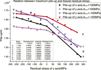
Pick out the maximum pile-up of both x and y axes from the simulation above, the relationship between the biaxial residual stress and the maximum pile-up along x and y axes can be obtained and is shown in Fig. 13. Linear fitting is used in the data processing. Slopes, intercepts, and their standard errors of the fits are also presented in Fig. 13.
Relations between maximum pile-up of x and y axes and residual stress after unloading: biaxial residual stress, along x-axis with a tensile stress of 100 MPa or compressive stress of 100 MPa, and along y-axis with stress changing from −250 to 250 MPa.

After a group of simulations with different parameters and different combinations of biaxial residual stress have been carried out, without consideration of friction, the formula of pile-up after unloading under the condition of biaxial residual stress can be concluded as:
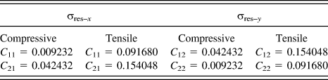
 $$\eqalign{ & {{{s_x}} \over {{s_0}}} = - {C_{11}}{{{\sigma _{{\rm{res}} - x}}} \over {{\sigma _{\rm{Y}}}}} - {C_{12}}{{{\sigma _{{\rm{res}} - y}}} \over {{\sigma _{\rm{Y}}}}} + 1 \cr & {{{s_y}} \over {{s_0}}} = - {C_{21}}{{{\sigma _{{\rm{res}} - x}}} \over {{\sigma _{\rm{Y}}}}} - {C_{22}}{{{\sigma _{{\rm{res}} - y}}} \over {{\sigma _{\rm{Y}}}}} + 1\quad , \cr}$$
where σres–x is the residual stress of x axis, σres–y is the residual stress of y axis, s x is the maximum pile-up of x axis, s y is the maximum pile-up of y axis, s 0 is the maximum pile-up without residual stress, and σY is the yield stress. According to the fitting curve, the constants C 11, C 12, C 21, and C 22 are as follows in Table I.
Constants from the fitting curves.

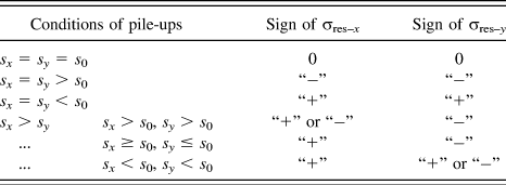
Before calculating biaxial residual stress by using Eq. (4), the full-field pile-up displacements after unloading should be measured firstly. Due to the symmetry, there are two maximum pile-up displacements. The direction of the connecting line of these two maximum pile-ups is the direction of the maximum residual stress component, and the vertical line of this connecting line corresponds to the minimum residual stress component. The coefficients C 11, C 12, C 21, and C 22 should be correctly selected according to the state of residual stress components. According to Eq. (4), we can determine most cases of residual stress components in the tensile or compression state with the help of different amplitude of pile-ups. The analyzed results are listed in Table II (“−” means compressive and “+” means tensile).
Signs of σres–x and σres–y determined by pile-ups.

Some signs of residual stress components are still in uncertainty for two cases of combination of pile-ups. However, the unique relationship between pile-ups after unloading and biaxial residual stress is helpful to settle this issue. Some values of residual stress components and pile-ups after unloading are shown in Table III calculated from Eq. (4). The four shadow regions in Table III are corresponding to the cases of discussed residual stresses. If the pile-ups in x and y axes are given, the signs of residual stress can be determined from Table III. Thus, the residual stress components will be accurately obtained from Eq. (4).
Relationship between the maximum pile-up and residual stress.

V. EXPERIMENTS AND ANALYSIS
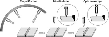
The specimen consisted of two blocks of steel (n = 0.1, σY = 400 MPa) with a size of 80 mm × 50 mm × 10 mm welded together before residual stress measurement, the welded specimen was polished to keep the surface smoothly. The surface residual stresses were firstly measured by the x-ray diffraction method before the indentation process. A Brinell indenter with a diameter of 2.5 mm was used to press on the selected point of the specimen and remained for 30 s. The welding zone is not the testing area in the method proposed here, the method is used to measure the residual stress of the base material after welding. After unloading, the information of remained permanent deformation can be measured to evaluate the surface residual stress from the above conclusion. The diagram of an experimental process is shown in Fig. 14.
Schematic diagram of experimental process.

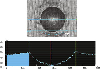
The parameter s 0 was measured by indentation experiment using the same material without residual stress before welding, s 0 = 164.6 μm. The pile-up morphology around the indentation can be obtained by a confocal microscopy system (VK-X200, made by Keyence, Osaka, Japan, resolution: 20 nm), and then the maximum pile-up can be determined (see Fig. 15). With the method proposed above, the corresponding residual stress can be obtained with Eq. (4) and Table III. The experimental results are in good agreement with those of x-ray tests, deviations of the out-of-plane displacement data result in the deviations of residual stress components, as listed in Table IV.
The pile-up morphology around an indentation.

Comparison of pile-up method and x-ray test.

From Eqs. (3)–(4), the variation of pile-up for a unit variation of stress is very small, especially for compressive residual stress. The sensitivity and accuracy of this method mainly depend on the resolution of the optical measuring system. The resolution of the confocal microscopy system used in the experiment is 20 nm. Assuming that the specimen is under uniaxial compressive residual stress, from the relationship between pile-up and residual stress, one can obtain
 $${{\Delta {s_x}} \over {{s_0}}} = - {C_{11}}{{\Delta {\sigma _{{\rm{res}}}}} \over {{\sigma _{\rm{Y}}}}}\quad ,$$
and C 11 = 0.009232. Take the steel mentioned above as an example, s 0 = 164.6 μm and σY = 400 MPa. According to Δs x = 20 nm, the sensitivity of the compressive residual stress determined by the method proposed here is 5.26 MPa. For uniaxial tensile stress, C 11 = 0.09168, the corresponding sensitivity value is 0.53 MPa. And for biaxial residual stress, the sensitivity value can also be determined when the directions of residual stress components are obtained by using Tables II and III. The method is effective and the sensitivity can satisfy the requirement of engineering and industry fields.
VI. CONCLUSION
In the present paper, a novel method for measuring residual stresses both in uniaxial and biaxial stress states is proposed. The relationship between the pile-up displacement around an indentation after unloading and the superficial residual stress in an object is firstly established with the help of finite element method. The direction of residual stress can be correctly determined by the unique relationship between pile-up after unloading and residual stress. The simulation fringe patterns are similar to the Underwood's experimental observation, and they are helpful to recognize the direction of residual stress. An experiment was set up to measure the pile-up displacement around the indentation and then the pile-up was transformed to the corresponding residual stress. The experimental results are in agreement with the numerical simulations and the x-ray test results. The method proposed here lays a strong foundation for measuring residual stress by pile-up displacements with instrument indentation in the near future.
ACKNOWLEDGMENTS
This work was financially supported by the NSFC (Nos. 11272131, 11472114), the Specialized Research Fund for the Doctoral Program of Higher Education of China (No. 20110142110039), and the Fundamental Research Funds for the Central Universities, HUST: No. 2013KXYQ008.