1 Introduction
There are many circumstances where fluids flow to the Earth’s surface from depth through regions of high permeability. This paper analyses the situation wherein compressible fluids discharge steadily through a permeable conduit from a pressurized reservoir. Examples include: magmatic volatiles being released from a magma chamber beneath an active volcano; discharges of geothermal fluids; and escape of natural gas and carbon dioxide (
 $\text{CO}_{2}$
) from natural or man-made sources. The volcanic case is relevant to understanding gas emissions at volcanoes, while the
 $\text{CO}_{2}$
case is of great concern to carbon capture and storage (CCS) where an uncontrolled gas escape would pose a significant hazard.
Flows of effectively incompressible fluids (such as magma and water) have been much studied. In steady state, the flow is driven by the pressure difference between that at depth and that at the surface and there is no difference between volume and mass conservation. Compressible flows are quite different; in particular the mass flux will be constant but the volume flux will vary strongly with pressure and hence depth. The relatively low pressure and density at the surface then indicate that the exit velocity is very much larger than that at depth. In fluid systems of geological interest, notably water and
 $\text{CO}_{2}$
, there may also be important changes in physical properties as the pressure changes from more liquid-like behaviour at high pressure to behaviour as a gas at low pressure below the supercritical point. There are also regions of two-phase flow for water, such as in geothermal systems (Woods & Fitzgerald Reference Woods and Fitzgerald1993; Pinder & Gray Reference Pinder and Grey2008).
Here we investigate the case of fluids at high temperature, which are strongly compressible at pressures in the upper crust. Our models are concerned with one-phase systems which are always at high enough temperature to avoid two-phase systems (water–vapour). Such situations will be considered in a later paper. A major, but not the only, motivation of the present study is degassing of volcanoes and flows of magmatic fluids during formation of metalliferous ore deposits. However, the theory developed, with some modifications, can be applied more widely.
The details are presented for a circular conduit of radius
 $a$
which may vary with the vertical coordinate
 $z$
. The results obtained can be taken over to flow in a two-dimensional permeable zone of width
 $W$
if the cross-sectional area
 $\unicode[STIX]{x03C0}a^{2}$
is replaced by
 $W$
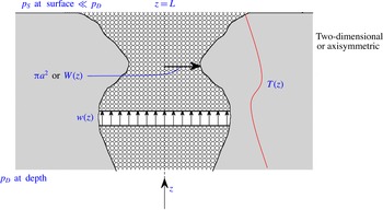
throughout (figure 1).
A sketch of the flow domain showing the vertical velocity,
 $w(z)$
, in a permeable medium bounded by an exterior solid with temperature
 $T(z)$
.

The time-independent vertical velocity
 $w$
in a porous medium is described by Darcy’s law (Bear Reference Bear1972; Phillips Reference Phillips1991; Woods Reference Woods2015) which is valid when the Reynolds number based on a representative pore size is less than approximately 10. For larger Reynolds numbers, inertial terms can be important and the flow is described by a nonlinear equation known as the Darcy–Forchheimer law (Bear Reference Bear1972; Dullien Reference Dullien1991). In our case, we consider here the locally low Reynolds number situation and write
 $$\begin{eqnarray}w=-(k/\unicode[STIX]{x1D707})\frac{\text{d}p}{\text{d}z},\end{eqnarray}$$
where
 $k$
, the permeability, and
 $\unicode[STIX]{x1D707}$
, the dynamic viscosity, may be considered constant or may vary with depth (and possibly in some cases with pressure,
 $p$
) and gravitational effects may be neglected due to the relatively low density of the gas – the flow is mainly driven by the pressure gradient, which is large compared to the gravitational contribution. In addition, we investigate effects due to change in conduit radius with depth. The initiation of the flow is at
 $z=0$
, at which point variables are designated by a subscript
 $D$
(for depth), and the vapour reaches the surface at
 $z=L$
, at which point variables are designated by a subscript
 $S$
(for surface). The analysis consists of finding an expression for the mass flux, which, while initially unknown in the calculation, is constant across each horizontal plane. This allows the determination of the governing differential equation for the pressure, which can be integrated to obey the conditions
 $$\begin{eqnarray}p=p_{D}\quad (z=0)\quad \text{and}\quad p=p_{S}\quad (z=L),\end{eqnarray}$$
and yields the necessary value of the mass flux
 $M$
and corresponding
 $w(z)$
. As indicated physically above,
 $w(L)\equiv w_{S}$
can be much larger than
 $w_{D}$
. We give some numerical values and graphical curves to illustrate this in § 3 after developing the general relationships in the next section.
Having evaluated the mass flux, we then determine the pressure field and finally an expression for the vertical velocity through the conduit. These relationships can then be used to determine various unknowns in real geological systems. For example, there are some measurements and estimates of mass flux at several volcanoes such as Montserrat in the Caribbean (Edmonds Reference Edmonds2008) and from models of magma chambers connected by conduits to volcanic craters (Christopher et al. Reference Christopher, Humphreys, Barclay, Genareau, de Angelis, Plail, Donovan, Wadge, Robertson and Voight2014). From these measurements and estimates and the theory developed here we can say more about variables such as permeability and conduit radius. We do so, in part, in § 4. Further analysis will be presented in a journal more devoted to the Earth sciences.
The ideas also have relevance to the sequestration of carbon dioxide, of great societal concern at the moment. Currently 37 billion tonnes of carbon dioxide are input annually into the atmosphere by mankind. This is believed to be gradually increasing the world-wide average global temperature at ground level, leading to increased droughts, flooding and deaths. One solution is to store the carbon dioxide at depth, at least until well past the fossil fuel era. Very roughly, some 10 million tonnes are being sequestered this way each year at the moment. One of the concerns is potential leakage of the carbon dioxide (Pritchard Reference Pritchard2007; Preuss Reference Preuss2008; Neufeld, Vella & Huppert Reference Neufeld, Vella and Huppert2009; Huppert & Neufeld Reference Huppert and Neufeld2014). If the leakage results in the supercritical carbon dioxide rising above its supercritical level some of the effects described in this paper could occur. Several natural events have shown that dense
 $\text{CO}_{2}$
discharges on the Earth’s surface can be highly hazardous (Kling et al.
Reference Kling, Clark, Compton, Devine, Evans, Humphrey, Lockwood and Tuttle1987).
2 Flow through a porous conduit
The constant mass flux
 $M$
across any horizontal surface is given by
 $$\begin{eqnarray}M=\unicode[STIX]{x03C0}a^{2}\unicode[STIX]{x1D70C}w,\end{eqnarray}$$
where
 $\unicode[STIX]{x1D70C}$
is the vapour density. Inserting (1.1) into (2.1), we see that
 $$\begin{eqnarray}M=-\unicode[STIX]{x03C0}a^{2}(k/\unicode[STIX]{x1D707})\unicode[STIX]{x1D70C}\frac{\text{d}p}{\text{d}z},\end{eqnarray}$$
which in steady state must be independent of
 $z$
.
2.1 Incompressible comparison
By way of contrast, consider, for this subsection only, that
 $\unicode[STIX]{x1D70C},k,\unicode[STIX]{x1D707}$
and
 $a$
are all constant (as for an incompressible liquid flowing in a conduit of constant radius). Then integration of (2.2) with (1.2) indicates that the pressure
 $p$
is given by the linear relationship
 $$\begin{eqnarray}p=p_{D}\left(1-\frac{\unicode[STIX]{x0394}p}{p_{D}}\cdot \frac{z}{L}\right)\approx p_{D}\left(1-\frac{z}{L}\right),\end{eqnarray}$$
where
 $\unicode[STIX]{x0394}p\equiv p_{D}-p_{S}$
and (2.3b
) is valid under the approximation that
 $$\begin{eqnarray}p_{D}\gg p_{S}.\end{eqnarray}$$
In this case, the vertical velocity
 $$\begin{eqnarray}w=-(k/\unicode[STIX]{x1D707})(\unicode[STIX]{x0394}p/L)\approx (k/\unicode[STIX]{x1D707})p_{D}/L\end{eqnarray}$$
and the constant mass flux
 $$\begin{eqnarray}M=\unicode[STIX]{x03C0}a^{2}(k/\unicode[STIX]{x1D707})\unicode[STIX]{x1D70C}\unicode[STIX]{x0394}p/L\approx \unicode[STIX]{x03C0}a^{2}(k/\unicode[STIX]{x1D707})\unicode[STIX]{x1D70C}p_{D}/L.\end{eqnarray}$$
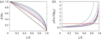
Non-dimensionalised graphs of
 $p/p_{D}$
and
 $\unicode[STIX]{x1D707}Lw/(kp_{D})$
are shown in figure 2.
(a) The non-dimensionalised pressure as a function of non-dimensionalised position along the conduit for: (i) an incompressible gas; (ii) a compressible gas with all quantities specifying it and the medium constant; (iii) a compressible gas satisfying (2.15) with
 $b=-1$
, 3 and 5; (iv) (2.16) with
 $c=-1$
and 1; and (v) an adiabatic rise with constant
 $h(z)$
in (2.21) for
 $\unicode[STIX]{x1D6FE}=5/3$
and
 $7/5$
. (b) The non-dimensionalised velocity as a function of non-dimensionalised position for the same parameter values as in (a).

2.2 Slow ascent; isothermal flow
If the ascent is sufficiently slow that the gas can thermally equilibrate to the surrounding temperature,
 $T(z)$
, which requires the ascent velocity to be much less than the speed of sound in the gas, the relationship between density and pressure is given by
 $$\begin{eqnarray}\unicode[STIX]{x1D70C}=\unicode[STIX]{x1D6FD}p/T,\end{eqnarray}$$
where
 $\unicode[STIX]{x1D6FD}$
is the molar mass divided by
 $R$
, the universal gas constant.
Inserting (2.7) into (2.2), assuming
 $a,k$
and
 $\unicode[STIX]{x1D707}$
are given functions of
 $z$
and integrating, we obtain the expression for the pressure
 $p$
, after use of (1.2a
) and rearrangement, of
 $$\begin{eqnarray}p=[p_{D}^{2}-2MF(z)]^{1/2},\end{eqnarray}$$
where, as a function of distance up the conduit,
 $$\begin{eqnarray}f(z)=\left(\frac{1}{\unicode[STIX]{x03C0}\unicode[STIX]{x1D6FD}}\right)\left(\frac{\unicode[STIX]{x1D707}T}{ka^{2}}\right)\quad \text{and}\quad F(z)=\int _{0}^{z}f(z^{\prime })\,\text{d}z^{\prime }.\end{eqnarray}$$
The functional form of
 $f(z)$
indicates how the possibly variable values of
 $k,\unicode[STIX]{x1D707},T$
and
 $a$
are reflected in the evaluation of the mass flux, vertical velocity and pressure distribution and that it is the combination
 $\unicode[STIX]{x1D707}T/ka^{2}$
that is important.
Using (1.2b ), we determine that
 $$\begin{eqnarray}M=\frac{1}{2F(L)}(p_{D}^{2}-p_{S}^{2})\approx \frac{p_{D}^{2}}{2F(L)}.\end{eqnarray}$$
It is thus the mean value of
 $\unicode[STIX]{x1D707}T/(ka^{2})$
that determines the resultant flux throughout the conduit and not the detailed distribution of any of these quantities. Inserting (2.10b
) into (2.8), we determine that
 $$\begin{eqnarray}\displaystyle p/p_{D} & {\approx} & \displaystyle [1-F(z)/F(L)]^{1/2}\end{eqnarray}$$
 $$\begin{eqnarray}\displaystyle & = & \displaystyle (1-z/L)^{1/2}\end{eqnarray}$$
if
 $f(z)$
is constant. A formula relating pressure to the square root of distance, similar to (2.12), was previously obtained by Mueller et al. (Reference Mueller, Melnik, Spider, Scheu and Dingwell2005), as their equation (2.8), to describe some high-pressure shock tube experiments with all parameters held constant. The relationship (2.12) is displayed in figure 2(a), which demonstrates graphically how different the result is from that for an incompressible liquid given by (2.3b
). The comparison between the pressure curves of figure 2(a) for the incompressible (liquid-like) and compressible (vapour-like) cases is due to the Darcy flow law expressed by (1.1). As compressible fluid rises, its vertical velocity increases (to conserve mass) and by (1.1) so must the pressure gradient. This indicates that, because the pressure is pinned to
 $p_{D}$
at
 $z=D$
and
 $p_{S}$
at
 $z=L$
, the only possible form for the pressure curve is the one shown, which is concave downwards. This must also be the situation for variable
 $f(z)$
, as demonstrated further below for some specific
 $f(z)$
.
Differentiating (2.8) and placing the result into (1.1), we find that
 $$\begin{eqnarray}\displaystyle w & {\approx} & \displaystyle \frac{kp_{D}}{2\unicode[STIX]{x1D707}}\frac{f(z)}{F(L)}\left(1-\left(1-\frac{p_{S}^{2}}{p_{D}^{2}}\right)\frac{F(z)}{F(L)}\right)^{-1/2}\end{eqnarray}$$
 $$\begin{eqnarray}\displaystyle & = & \displaystyle \frac{kp_{D}}{2\unicode[STIX]{x1D707}L}\left(1-\left(1-\frac{p_{S}^{2}}{p_{D}^{2}}\right)\frac{z}{L}\right)^{-1/2},\end{eqnarray}$$
where (2.14) follows from (2.13) if
 $f(z)$
is constant, as shown in figure 2(b). The velocity of the vapour becomes very large as the surface is approached because of the low pressure there.
In general circumstances, or in particular in the Earth, the four parameters
 $k,\unicode[STIX]{x1D707},T$
and
 $a$
could be individually constant or vary with depth. A linear representation of
 $a$
and
 $T$
with depth pertains to many geological situations, while as a generalisation
 $k$
varies exponentially in the Earth’s upper crust (Kuang & Jiao Reference Kuang and Jiao2014). All four parameters, especially
 $k$
, may also be functions of the pressure
 $p$
, as considered further below.
Suppose then, by way of illustration, the parameters in (2.9a
), and in particular the combination
 $\unicode[STIX]{x1D707}T/ka^{2}$
, vary with distance in such a way that there is a linear change in
 $f$
with distance. Then we can write
 $$\begin{eqnarray}f(z)=f_{D}(1+bz/L)\quad \text{and}\quad F(z)=f_{D}\left(z+{\textstyle \frac{1}{2}}bz^{2}/L\right)\end{eqnarray}$$
for some
 $b$
with
 $-1<b$
(because
 $f$
must be always positive).
Figure 2 includes corresponding curves for
 $p$
and
 $w$
for various values of
 $b$
. Note that if
 $b=-1$
(
 $f$
decreases, linearly, to zero at the surface), the results for the incompressible, constant radius case are retrieved. Thus if there is a linear decrease to zero in the quotient
 $\unicode[STIX]{x1D707}T/(ka^{2})$
, no matter how the individual parameters vary, the pressure field compensates to be linear and the density of the vapour remains constant.
Alternatively, if
 $$\begin{eqnarray}f(z)=f_{D}\text{e}^{-cz/L}\quad \text{then}~F(z)=L\frac{f_{D}}{c}(1-\text{e}^{-c/L}).\end{eqnarray}$$
Solution curves for various values of
 $c$
are also presented in figure 2. The differences for various values of
 $b$
and
 $c$
are topologically relatively small compared with the result for an incompressible gas.
As indicated above some of the parameters, particularly the permeability
 $k$
, could be functions of pressure, as well as possibly
 $z$
. The first-order nonlinear eigenvalue equations (2.2), (2.7) with boundary conditions (1.2) are still solvable analytically. Since, alternatively, an iterative scheme, with functions of pressure being written in terms of the previously obtained function of pressure in terms of
 $z$
, could be pursued, the overall result is that the shape of the pressure as a function of depth must be the same.
2.3 Rapid ascent; adiabatic flow
In the extreme case where the ascent is adiabatic because there is not sufficient time for there to be appreciable heat transfer from the gas to the surroundings, which will occur if the flow speed is not small compared to the speed of sound in the gas, the relationship between density and pressure is given by
 $$\begin{eqnarray}\unicode[STIX]{x1D70C}=Cp^{1/\unicode[STIX]{x1D6FE}},\end{eqnarray}$$
where
 $\unicode[STIX]{x1D6FE}$
is the ratio of the specific heat at constant pressure to that at constant volume (typically
 $5/3\approx 1.67$
for a monotonic gas and
 $7/5\approx 1.4$
for a diatomic gas) and
 $$\begin{eqnarray}C=\unicode[STIX]{x1D70C}_{D}/p_{D}^{1/\unicode[STIX]{x1D6FE}}=\unicode[STIX]{x1D6FD}p_{D}^{1-1/\unicode[STIX]{x1D6FE}}/T_{D}.\end{eqnarray}$$
Proceeding as before, on the assumption that Darcy’s flow law is still valid for such large velocities (Bear Reference Bear1972), we find that
 $$\begin{eqnarray}M=\unicode[STIX]{x03C0}a^{2}C^{1/\unicode[STIX]{x1D6FE}}\cdot p^{1/\unicode[STIX]{x1D6FE}}u=-\unicode[STIX]{x03C0}a^{2}C^{1/\unicode[STIX]{x1D6FE}}\left(\frac{k}{\unicode[STIX]{x1D707}}\right)p^{1/\unicode[STIX]{x1D6FE}}\frac{\text{d}p}{\text{d}z}.\end{eqnarray}$$
Thus
 $$\begin{eqnarray}\displaystyle p/p_{D} & {\approx} & \displaystyle [1-H(z)/H(L)]^{\unicode[STIX]{x1D6FE}/(1+\unicode[STIX]{x1D6FE})}\end{eqnarray}$$
 $$\begin{eqnarray}\displaystyle & = & \displaystyle (1-z/L)^{\unicode[STIX]{x1D6FE}/(1+\unicode[STIX]{x1D6FE})}\end{eqnarray}$$
if
 $h(z)$
is constant, as shown in figure 2(a), where
 $$\begin{eqnarray}h(z)=\frac{\unicode[STIX]{x1D707}}{\unicode[STIX]{x03C0}a^{2}kC}\quad \text{and}\quad H(z)=\int _{0}^{z}h(z^{\prime })\,\text{d}z^{\prime }\end{eqnarray}$$
and hence
 $$\begin{eqnarray}\displaystyle M & = & \displaystyle \left(\frac{\unicode[STIX]{x1D6FE}}{1+\unicode[STIX]{x1D6FE}}\right)\frac{1}{H(L)}\left(p_{D}^{1+1/\unicode[STIX]{x1D6FE}}-p_{S}^{1+1/\unicode[STIX]{x1D6FE}}\right)\end{eqnarray}$$
 $$\begin{eqnarray}\displaystyle & {\approx} & \displaystyle \left(\frac{\unicode[STIX]{x1D6FE}}{1+\unicode[STIX]{x1D6FE}}\right)\frac{1}{H(L)}p_{D}^{1+1/\unicode[STIX]{x1D6FE}}.\end{eqnarray}$$
Also
 $$\begin{eqnarray}\displaystyle w & {\approx} & \displaystyle \frac{\unicode[STIX]{x1D6FE}K}{(1+\unicode[STIX]{x1D6FE})\unicode[STIX]{x1D707}}p_{D}\frac{h(z)}{H(L)}\left[1-\left(1-\frac{p_{S}^{2}}{p_{D}^{2}}\right)\frac{H(z)}{H(L)}\right]\end{eqnarray}$$
 $$\begin{eqnarray}\displaystyle & = & \displaystyle \frac{\unicode[STIX]{x1D6FE}Kp_{D}}{(1+\unicode[STIX]{x1D6FE})\unicode[STIX]{x1D707}}\left[1-\left(1-\frac{p_{S}^{2}}{P_{D}^{2}}\right)\frac{z}{L}\right]^{-1/(1+\unicode[STIX]{x1D6FE})}\end{eqnarray}$$
if
 $h(z)$
is constant, which is shown in figure 2(b).
When the flow is slow the temperature taken by the gas in determined by the external temperature, cf. (2.9a ). When the expansion is adiabatic there is no cross-stream thermal transfer and the temperature is given, from (2.7), (2.17) and (2.23) by
 $$\begin{eqnarray}\displaystyle T & {\approx} & \displaystyle T_{D}\left[1-\left(1-\frac{p_{S}^{2}}{P_{D}^{2}}\right)H(z)/H(L)\right]\end{eqnarray}$$
 $$\begin{eqnarray}\displaystyle & = & \displaystyle T_{D}(1-z/L)^{(\unicode[STIX]{x1D6FE}-1)/(\unicode[STIX]{x1D6FE}+1)}\end{eqnarray}$$
if
 $h(z)$
is constant and
 $p_{S}\ll p_{D}$
.
Since for all our calculations, except the incompressible case (2.3), the pressure gradient is very large near
 $z=0$
, the pressure must be always larger for some range
 $0<z<z_{D}$
than any linear external pressure gradient with the same value,
 $p_{S}$
, at
 $z=0$
. This leads to a key issue in considering flows of a compressible fluid to the Earth’s surface, which is the contrast between the pressure in the vapour and the pressure in rocks surrounding the permeable pathway. In the case of impermeable, zero porosity surroundings the only relevant pressure contrast is between the fluid pressure and the lithostatic pressure (the pressure in the external rocks). The most straightforward case is when
 $p_{D}$
, the fluid pressure at the source
 $(z=0)$
equals the external lithostatic pressure, say
 $p_{L}$
, there. The case of
 $p_{D}$
greater than
 $p_{L}$
is geologically important, with overpressures limited by rock strength and the state of deviatoric stress. In some geological situations, in contrast,
 $p_{D}<p_{L}$
. In this case there will be underpressures at depth and overpressures at shallower levels with a crossover point.
Suppose, for simplicity and means of illustration, we consider the (isothermal, constant parameters) pressure given by (2.12) and compare it with an external linear pressure field, given by
 $$\begin{eqnarray}p_{e}=p_{L}-(p_{L}-p_{S})(z/L).\end{eqnarray}$$
Then
 $p>p_{e}$
for
 $z/L<1-(p_{D}/p_{L})^{2}=0.84$
if
 $p_{D}/p_{L}=0.4$
(and
 $p_{S}\ll p_{L}$
), as might be for a geological situation. The difference between the fluid and lithostatic pressure reaches a maximum at some intermediate depth which for our simple illustrative case occurs at
 $z/L=1-(1/4)(p_{D}/p_{L})^{2}=0.96$
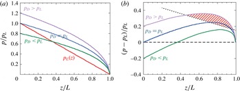
(figure 3). Since rock strength increases with depth we can also predict a zone of rock failure where the overpressure exceeds the strength (figure 3).
(a) Schematic plot of the typical variation of pressure with depth for the pressure in the conduit,
 $p_{D}$
, at
 $z=0$
: (1) equal to; (2) greater than; and (3) less than, the external, lithostatic pressure
 $p_{L}$
there. (b) The difference between internal and external pressures (fluid and lithostatic) for the three cases in (a). The overpressure reaches a maximum at intermediate depths in all cases. For
 $p_{0}\leqslant p_{L}$
the fluid is overpressured at all depths. If
 $p_{D}<p_{L}$
(as in a hydrostatic compressible fluid reservoir) the fluid is underpressured at depth but will become overpressured at shallower depths. The dashed line presents a possible variation of rock strength with depth and indicates the possibility of a fracture zone being developed when fluid pressure exceeds the strength of the surrounding rocks.

In geological environments a fast high permeability pathway will be embedded in lower permeability and typically lower porosity host rock. In this case the ambient fluid in the host rock may be at hydrostatic pressure, which is typically approximately 30–40 % of the lithostatic pressure. The high fluid pressures in the flow along the high permeability pathway can therefore greatly exceed the hydrostatic pressure and as a consequence the fluid will move laterally into the low permeability host rock. Alternatively, there may be a region at depth where the pressure in the fluid is less than that externally at the same depth. In the lower region, fluid from the external interstices will be sucked into the flow, as envisaged necessary for the new theory of porphyry copper formation (Blundy et al. Reference Blundy, Mavrogenes, Tattich, Sparks and Gilmer2015).
We now consider two different geological situations to illustrate some of the implications of these pressure differences.
3 Numerical values
The curves in figure 2 give some indication of some of the quantitative effects of compressibility. We now present two quantitative indications. First, we consider discharge of magmatic fluids released from the top of a magma chamber. Applications of this case pertain to both degassing of volcanoes and formation of porphyry copper deposits. A widely invoked scenario is a magma chamber at approximately 5 km depth releasing magmatic fluid that has a pressure equal to or slightly above lithostatic pressure, in which case tensile fractures need to form to provide the route to escape. Assuming, for the sake of this illustration, that all quantities are constant and given by:
 $k=10^{-14}~\text{m}^{2}$
;
 $\unicode[STIX]{x1D707}=2\times 10^{-5}~\text{Pa}~\text{s}$
;
 $p_{D}=10^{8}~\text{Pa}$
;
 $p_{S}=10^{5}~\text{Pa}$
;
 $a=100~\text{m}$
;
 $T=850\,^{\circ }\text{C}$
;
 $\unicode[STIX]{x1D6FD}=2.17\times 10^{-3}~\text{kg}~\text{K}~\text{Pa}^{-1}~\text{m}^{-3}$
; and
 $L=5\times 10^{3}~\text{m}$
, we find from (2.10b
) that
 $M=30~\text{kg}~\text{s}^{-1}\approx 2.6\times 10^{6}~\text{kg}~\text{day}^{-1}$
and from (2.14)
 $w_{S}=5\times 10^{-3}~\text{m}~\text{s}^{-1}$
and
 $w_{D}=5\times 10^{-6}~\text{m}~\text{s}^{-1}$
. This evaluated flux is within the range of measurements of gas flux from many volcanoes (Edmonds Reference Edmonds2008).
As a second numerical example, we consider the possible leak from a carbon dioxide (
 $\text{CO}_{2}$
) storage reservoir. So far no such leaks have been reported, but it is conceivable, and needs to be understood for safety purposes, what would happen if there was an accidental leak through the (supposed to be) containing cap rock (see Huppert & Neufeld (Reference Huppert and Neufeld2014) and references therein for further background). The
 $\text{CO}_{2}$
is compressed before storage beyond the supercritical point so it behaves like a liquid (with relatively small specific volume). A leak from the confining reservoir of the relatively light
 $\text{CO}_{2}$
could result in it rising through the overlying porous medium to be confined by another cap rock. The worst scenario is that it rises above the supercritical point and then, as a gas, rises all the way to the surface through a relatively permeable medium, such as a fault or fracture. For illustrative purposes, assume again that all quantities are constant and given by:
 $k=10^{-12}~\text{m}^{2}$
;
 $\unicode[STIX]{x1D707}=10^{-5}~\text{Pa}~\text{s}$
;
 $p_{D}=2\times 10^{7}~\text{Pa}$
;
 $p_{S}=10^{5}~\text{Pa}$
;
 $a=1~\text{m}$
;
 $T=50\,^{\circ }\text{C}$
;
 $\unicode[STIX]{x1D6FD}=2.17\times 10^{-3}~\text{kg}~\text{K}~\text{Pa}^{-1}~\text{m}^{-3}$
; and
 $L=10^{3}~\text{m}$
. Then from (2.10b
)
 $M=0.4~\text{kg}~\text{s}^{-1}\approx 3.7\times 10^{4}~\text{kg}~\text{day}^{-1}$
(very roughly 1 % of the current input rate at Sleipner,
 $w_{D}=10^{-3}~\text{m}~\text{s}^{-1}$
and
 $w_{S}=0.2~\text{m}~\text{s}^{-1}$
. If instead,
 $a$
is taken to be 100 m and all other parameter values kept the same,
 $M=4\times 10^{3}~\text{kg}~\text{s}^{-1}\approx 3.7\times 10^{7}~\text{kg}~\text{day}^{-1}$
(
 ${\sim}$
two orders of magnitude larger than the current input rate at Sleipner), while neither
 $w_{D}$
nor
 $w_{S}$
is altered.
4 Summary
We have analysed the steady motion of a compressible gas, flowing either isothermally or adiabatically through a porous conduit allowing for parameters to vary along the flow. The results indicate that whatever the form of
 $f(z)$
, as defined by (2.29), the pressure at any point within the flow exceeds that if the flow was incompressible. Because the mass (and not volume flux) is constant along the conduit, the gas velocity increases along the flow. Our model will find application to various areas of concern in the Earth sciences. These include: the release of volcanic volatiles into a conduit connecting a magma chamber to the volcano above it; the discharge of geothermal fluids within the Earth’s crust, which lead to many ore deposits, such as porphyry copper; and the accidental release of carbon dioxide from a CCS reservoir. We presented two numerical examples to give some feeling for the magnitude of the various effects. A characteristic of our general results in that either large overpressures or underpressures can develop between the ascending fluid and the confining rocks dependent on explicit parameter values. These over- or underpressures are a consequence of the nonlinear pressure gradient which can arise in compressible fluids, as described in part by Melnik & Sparks (Reference Melnik and Sparks1999).
Acknowledgements
We are grateful to J. Blundy, C. Jaupart, O. Melnik (who pointed out Mueller et al. Reference Mueller, Melnik, Spider, Scheu and Dingwell2005) and A. Rust for comments on an earlier version of this manuscript. The research was undertaken while H.E.H. held a Leverhulme Emeritus Fellowship, for which he is grateful. The research of R.S.J.S. is partially supported by the European Research Council in the VOLDIES project.