1. Introduction
Fluid–structure interaction (FSI) is fundamental to understanding blood flow in the cardiovascular system. Research in this area spans theoretical, experimental and computational approaches. Theoretical studies have provided analytical insights into pulsatile flow in elastic vessels (Womersley Reference Womersley1955a ; Papadakis Reference Papadakis2011; Flores Geronimo et al. Reference Flores Geronimo, Alastruey and Corvera2016; Wu & Zhu Reference Wu and Zhu2023). Experimental work (Gerrard Reference Gerrard1985; Bessems et al. Reference Bessems, Giannopapa, Rutten and van de Vosse2008; Stojadinović et al. Reference Stojadinović, Tenne, Zikich, Rajković, Milošević, Lazović and Žikić2015) has validated these models through direct measurements of wave characteristics. Computational studies (Sherwin et al. Reference Sherwin, Franke, Peiró and Parker2003; Reymond et al. Reference Reymond, Merenda, Perren, Rüfenacht and Stergiopulos2009; Ghigo, Fullana & Lagrée Reference Ghigo, Fullana and Lagrée2017; Krul & Bagchi Reference Krul and Bagchi2025) have used numerical techniques to simulate flow and wall interactions in complex geometries, offering detailed insights into the wave dynamics and energy transmission.
Theoretical studies often employ idealised models that simplify the vascular system by assuming axisymmetry and adopting the long-wave approximation. These analytical models are typically formulated and solved in the frequency domain, with time-domain responses efficiently reconstructed using the inverse Fourier transform. This approach enables rapid haemodynamic assessment without the need to numerically solve differential equations (Papadakis & Raspaud Reference Papadakis and Raspaud2019; Wu & Zhu Reference Wu and Zhu2023). The models can be broadly classified based on how their governing equations are derived. One class is derived by linearising the Navier–Stokes (N–S) equations in terms of primitive variables and coupling them with linear elastodynamic equations (Womersley Reference Womersley1955a ; Atabek & Lew Reference Atabek and Lew1966; Cox Reference Cox1968). The other is based on linearised, cross-sectionally averaged (one-dimensional) N–S equations coupled with a tube law (Alastruey et al. Reference Alastruey, Passerini, Formaggia and Peiró2012; Wiens & Etminan Reference Wiens and Etminan2021; Fancher & Katifori Reference Fancher and Katifori2022).
Analytical modelling of the effect of fluid viscosity can be challenging and heavily influenced by how the governing equations are formulated. In the first class of frequency-domain solutions, viscosity is naturally incorporated, as the radial velocity distribution is explicitly resolved. In contrast, the second class solves directly for flow rate, and viscous effects must be approximated a posteriori, typically by assuming a Womersley velocity profile or applying frequency-dependent friction models (Zielke Reference Zielke1968). The role of fluid viscosity in wave propagation has been the subject of extensive research. Womersley (Reference Womersley1955a ) demonstrated that fluid viscosity reduces the wave speed and attenuates wave transmission, with the degree of attenuation strongly dependent on frequency. Jones et al. (Reference Jones, Anliker and Chang1971) conducted a parametric analysis of wave propagation in viscous fluid-filled elastic tubes and identified two types of waves: fast waves and slow waves, each responding differently to viscous effects. The fast wave is primarily influenced by dispersion, while the slow wave experiences significant damping due to viscosity. Giusti & Mainardi (Reference Giusti and Mainardi2016) incorporated the frictional term from Womersley’s solution and employed a Laplace transform to show that uni-axial wave propagation in a fluid-filled elastic tube behaves analogously to wave propagation in a viscoelastic solid. Stojadinović et al. (Reference Stojadinović, Tenne, Zikich, Rajković, Milošević, Lazović and Žikić2015) conducted experiments measuring the pulse-wave velocity (PWV) in elastic tubes with varying fluid viscosity, confirming that PWV decreases as viscosity increases. Žikić & Žikić (Reference Žikić and Žikić2022) derived asymptotic expressions for wave speed in the limits of low and high fluid viscosity and validated their findings experimentally.
Solid viscosity, reflecting the viscoelastic properties of the arterial wall, can also play a key role in haemodynamics. In analytical models, wall viscosity is typically introduced by either extending elastodynamic equations to a viscoelastodynamic form using the Kelvin–Voigt or standard linear solid models (Chow & Apter Reference Chow and Apter1968), or by representing it as a phase angle in transmission line theory (Taylor Reference Taylor1966). Both dispersion and dissipation effects due to wall viscosity have been well documented. Womersley (Reference Womersley1957a ), expanding upon the work of Morgan & Kiely (Reference Morgan and Kiely1954), introduced wall viscosity by substituting the elastic constants (Young’s modulus and Poisson’s ratio) with complex-valued counterparts. Their approximation indicated that wall viscosity results in a slight increase in wave speed and a significant enhancement of attenuation. This was later supported experimentally by Taylor (Reference Taylor1959), who showed that arterial wall viscoelasticity can be characterised independently of blood properties. Demiray & Akgün (Reference Demiray and Akgün1997) derived a dispersion relation incorporating wall viscosity and proved that dispersion persists even in the inviscid fluid limit. Ma & Ng (Reference Ma and Ng2009) showed that wall viscosity rapidly damps the time-averaged motion of the tube using perturbation analysis. In computational work, Reymond et al. (Reference Reymond, Merenda, Perren, Rüfenacht and Stergiopulos2009) demonstrated through one-dimensional (1-D) simulations that the physiological wall viscosity contributes to haemodynamic behaviour at the same order as convective acceleration and wall friction. Abdessalem et al. (Reference Abdessalem, Abdessalem, Salah and Mansouri2010) and Khaled & Saber (Reference Khaled, Saber, Dössel and Schlegel2010) utilised the 1-D wave equation and Womersley’s wave speed to calculate the input impedance of a straight viscoelastic tube at different frequencies, concluding that the frequency-dependent oscillations in the input impedance spectrum are considerably reduced by increasing the fluid and wall viscosity.
While current theoretical studies have deepened our understanding of the role of fluid or solid viscosities in wave propagation, they are often limited by restrictive assumptions; notably, they assume the solution is reflection free and harmonic in both time and space. However, several critical physiological features that can lead to the violation of these assumptions remain unaddressed. First, the vessel geometry is assumed to be cylindrical in most previous works, while real vessels are tapered. This tapering induces continuous reflections throughout the domain, meaning the wave is no longer spatially harmonic and a simple dispersion equation cannot be derived (Mynard & Kondiboyina Reference Mynard and Kondiboyina2022). This issue was not addressed until the analytical solution proposed by Papadakis (Reference Papadakis2011). Second, previous models often assume uniform material properties, which fail to capture realistic wall motion and wave speed. Third, most prior work employs a semi-infinite domain without proper boundary conditions to model wave reflections, which are critical in physiological wave propagation. Gerrard (Reference Gerrard1985) showed experimentally that Womersley’s theory breaks down near the reflecting outlet. More recently, Roknujjaman et al. (Reference Roknujjaman, Kyotoh, Yohei and Yasuhisa2023) observed a significant increase in wave amplitude caused by reflections at the tube exit. The analytical integration of the above three features is first addressed in the recent work of Wu & Zhu (Reference Wu and Zhu2023), which examined the input impedance of inviscid flow in an elastic tapered tube and found that its characteristics are highly sensitive to boundary conditions and tapering. However, the viscous effects from both the fluid and the wall are omitted in the works of Papadakis (Reference Papadakis2011) and Wu & Zhu (Reference Wu and Zhu2023). It is unclear how these viscosities will affect the dispersion and dissipation of the pulse wave.
From the above discussion, it is evident that despite advances in theoretical modelling, most studies overlook reflections stemming from tapering and boundary conditions. Moreover, because no well-established analytical model exists for tapered configurations, it remains to be explored how the combined influence of fluid and solid viscosities affects wave propagation, dispersion and dissipation in tapered tubes. To overcome these limitations, we developed a semi-analytical FSI model that captures the interaction between a viscous fluid and a viscoelastic wall, while considering important factors such as tapering, spatially varying material properties and boundary conditions.
This paper is organised as follows: § 2 formulates the problem, including the governing equations for the fluid and wall, along with coupling conditions. Section 3 presents the semi-analytical solution procedure and validates it against three-dimensional (3-D) simulation results. Section 4 analyses the influence of viscosity on key aspects of wave propagation. Finally, § 5 concludes the study, outlining key findings, limitations and future directions.
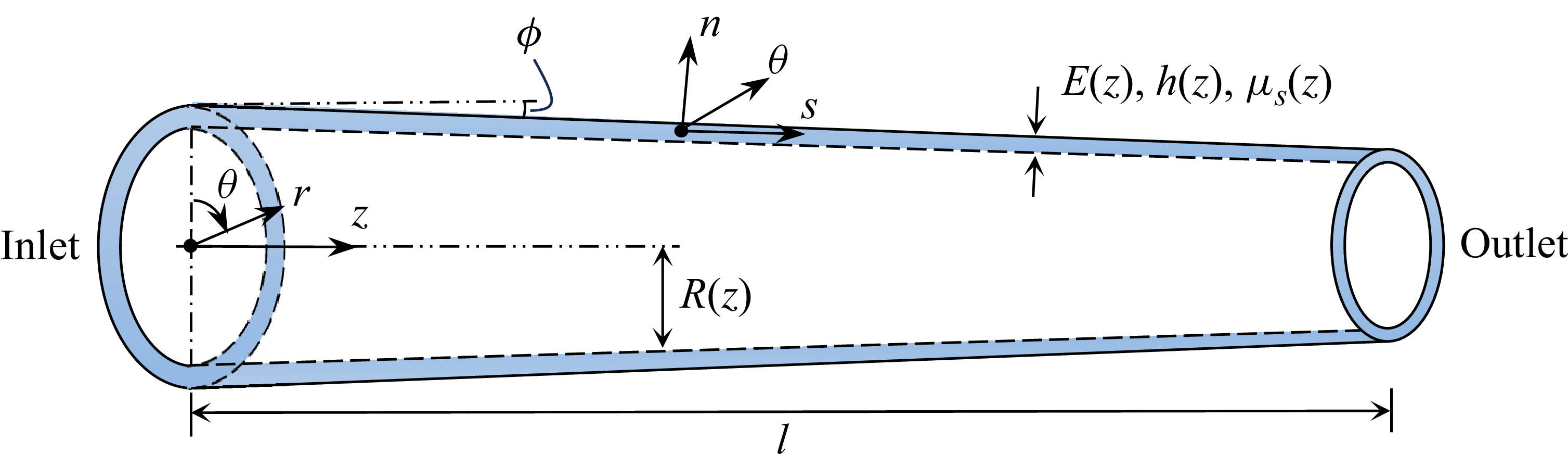
Schematic of a tapered viscoelastic tube filled with a viscous fluid, with wall properties that vary along the
 $z$
-direction. Here,
 $E$
is the elastic modulus,
 $h$
is the wall thickness, and
 $\mu_s$
is the solid viscosity.

2. Problem statement
In this section, we derive the governing equations and boundary conditions for the wave propagation of viscous fluid within tapered, viscoelastic tubes.
2.1. Configuration and kinematics
The blood vessel is modelled as an axisymmetric, linearly tapered tube, as illustrated in figure 1. The lumen radius varies along the axial coordinate
 $z$
and is described by the following equation:
 \begin{equation} R(z) = R_0 - bz, \end{equation}
where
 $R_0$
is the radius of the inlet,
 $b$
is the taper slope and
 $z \in [0,l]$
with
 $l$
being the tube length. The value of
 $b$
is small for arteries and typically does not exceed 0.026 (Segers & Verdonck Reference Segers and Verdonck2000). The vessel wall is modelled as a thin-walled, linear viscoelastic membrane undergoing small deformations. Under the small-strain assumption, the reference configuration is considered fixed, and thus the radius
 $R$
is treated as time-independent for the purpose of defining the fluid domain. While the domain boundary is non-moving, the wall undergoes infinitesimal displacements at
 $r=R$
, which are coupled to the fluid velocity. To facilitate the analysis, in addition to the global cylindrical coordinate system
 $(\boldsymbol{e}_r, \boldsymbol{e}_\theta , \boldsymbol{e}_z)$
, a local coordinate system
 $(\boldsymbol{e}_n, \boldsymbol{e}_\theta , \boldsymbol{e}_s)$
is introduced, where
 $\boldsymbol{e}_n$
and
 $\boldsymbol{e}_s$
denote the normal and tangential directions of the vessel wall, respectively. Both the local and global coordinate systems are illustrated in figure 1. The angle between the
 $z$
-direction and the
 $s$
-direction is denoted by
 $\phi$
, and the following relations are used to facilitate the transformation between the two coordinate systems:
 \begin{equation} \sin {\phi }=-\frac {{\textrm d} R}{{\textrm d} z} \Bigg/ \sqrt {\left ( \frac {{\textrm d} R}{{\textrm d} z} \right )^2 + 1 }=\frac {b}{\sqrt {b^2 + 1 }}, \quad \cos {\phi }=1/\sqrt {\left ( \frac {{\textrm d} R}{{\textrm d} z} \right )^2 + 1 }=\frac {1}{\sqrt {b^2 + 1 }}. \end{equation}
The radial and longitudinal displacements of the vessel wall in the global coordinate system are denoted by
 $u^w_r$
and
 $u^w_z$
, respectively, while
 $u^w_n$
and
 $u^w_s$
represent the wall displacements in the normal and tangential directions of the local coordinate system. We follow this convention and use the superscript
 $(\boldsymbol{\cdot })^w$
to denote wall-related quantities hereafter. Using (2.2), we have
 \begin{align} u^w_n &= \frac {1}{\sqrt {b^2+1}}u_r^w+\frac {b}{\sqrt {b^2+1}}u_z^w, \end{align}
 \begin{align} u^w_s &= -\frac {b}{\sqrt {b^2+1}}u_r^w+\frac {1}{\sqrt {b^2+1}}u_z^w. \\[10pt] \nonumber \end{align}
Experimental studies have shown that longitudinal movement of the vessel wall is negligible due to the strong bond between artery and perivascular tissues (Nichols, O’Rourke & Vlachopoulos Reference Nichols, O’Rourke and Vlachopoulos2011; Ferruzzi et al. Reference Ferruzzi, Di Achille, Tellides and Humphrey2018). To model this tethering effect, we follow the approach of Womersley (Reference Womersley1957b
) and Papadakis (Reference Papadakis2011), imposing a constraint on the wall in the tangential direction by setting
 $u^w_s = 0$
. Hence, (2.3) leads to
 \begin{align} u^w_n &= \sqrt {b^2+1}u_r^w, \end{align}
 \begin{align} u_z^w &= b u_r^w. \end{align}
At the fluid–structure interface, we enforce the no-slip condition through the following kinematic relationship:
 \begin{equation} v_r^w = v_r |_{r=R} = \frac {\partial u^w_r}{\partial t},\quad v_z^w = v_z |_{r=R} = \frac {\partial u^w_z}{\partial t}, \end{equation}
where
 $v_r$
and
 $v_z$
are the radial and axial fluid velocities, respectively.
2.2. Fluid–structure interaction
The equation governing the wall motion is given by (see Appendix A for detailed derivation)
 \begin{equation} \rho _s \frac {\partial ^2 u_n^w}{\partial t^2}=-\frac {\sigma _{\theta \theta }}{R\sqrt {1+b^2}}+F_n. \end{equation}
Here,
 $\rho _s$
,
 $F_n$
and
 $\sigma _{\theta \theta }$
denote the wall density, the normal component of the body force and the circumferential stress in the local coordinate system, respectively. We model the viscoelastic vessel wall using a linear Kelvin–Voigt material model (Alastruey et al. Reference Alastruey, Khir, Matthys, Segers, Sherwin, Verdonck, Parker and Peiró2011). The constitutive relation in the local coordinate system is given below, with the full derivation provided in Appendix A
 \begin{equation} \sigma _{\theta \theta } = \frac {1}{R\sqrt {1+b^2}\big(1-\nu ^2\big)} \left ( E u_n^w + \mu _s\frac {\partial u_n^w}{\partial t} \right ), \end{equation}
where
 $E$
is the elastic modulus,
 $\mu _s$
is the solid viscosity and
 $\nu$
is Poisson’s ratio. The material properties may vary along the axial direction and are treated as functions of
 $z$
. The wall deformation is driven by a body force
 $\boldsymbol{F}$
, which is defined as the surface traction exerted by the fluid on the wall divided by the wall thickness
 $h$
(Womersley Reference Womersley1955a
; Figueroa et al. Reference Figueroa, Vignon-Clementel, Jansen, Hughes and Taylor2006)
 \begin{equation} \boldsymbol{F} =\frac {-\boldsymbol{S} \boldsymbol{\cdot }\boldsymbol{e}_n}{h}. \end{equation}
Here,
 $\boldsymbol{S}$
is the Cauchy stress tensor of fluid. Based on the scale analysis in Appendix B, we have
 \begin{equation} S_{rr} \approx -p, \quad S_{zz} \approx -p, \quad S_{rz} \approx \mu _f\frac {\partial v_z}{\partial r}, \end{equation}
where
 $p$
is the fluid pressure, and
 $\mu _f$
is the dynamic viscosity of fluid. The normal component of the force acting on the wall is given by
 \begin{equation} F_n = \boldsymbol{F}\boldsymbol{\cdot }\boldsymbol{e}_n=\frac {1}{\big(1+b^2\big)h}\left ( -2bS_{rz} - S_{rr} - b^2S_{zz} \right ). \end{equation}
Substituting (2.4a ), (2.7), (2.9) and (2.10) into (2.6), we obtain the FSI relation incorporating fluid and solid viscosity
 \begin{align} p =\frac {1}{\sqrt {1+b^2}}\frac {Eh}{1-\nu ^2}\frac {u_r^w}{R^2} +\frac {1}{\sqrt {1+b^2}}\frac {\mu _s h}{1-\nu ^2}\frac {v_r^w}{R^2} + \nonumber \\ \frac {2b\mu _f}{1+b^2}\frac {\partial v_z}{\partial r}\bigg |_{r=R} +\rho _sh\sqrt {1+b^2}\frac {\partial v_r^w}{\partial t}. \end{align}
Equation (2.11) relates the fluid pressure and axial velocity to the wall’s radial displacement and velocity, serving as a complementary relation to close the FSI system. It reveals that tapering of the tube introduces an additional fluid viscous term, which vanishes when the tube is straight (
 $b = 0$
). Additionally, the last term in the equation represents the inertial contribution of the wall motion, which is negligible under the long-wave approximation (see Appendix B). When the tapering effect is neglected, (2.11) reduces to the classical 1-D viscoelastic tube law (Alastruey et al. Reference Alastruey, Khir, Matthys, Segers, Sherwin, Verdonck, Parker and Peiró2011)
 \begin{equation} p=\frac {Eh}{1-\nu ^2}\frac {u_r^w}{R^2}+\frac {\mu _s h}{1-\nu ^2}\frac {v_r^w}{R^2}. \end{equation}
2.3. Governing equations and boundary conditions
The blood in the modelled artery is treated as an incompressible Newtonian fluid governed by the axisymmetric N–S equations without body forces. To further simplify the system, the long-wave approximation is commonly employed, assuming that the characteristic axial length scale is much greater than the radial one, and that the wave speed is much larger than the axial flow velocity (Womersley Reference Womersley1957a ; Filonova et al. Reference Filonova, Arthurs, Vignon-Clementel and Figueroa2020). Under these assumptions, a scale analysis is conducted in Appendix B, showing that nonlinear terms and the radial variation of pressure can be neglected. Additionally, the inertial contribution of the wall motion is also negligible. Finally, we summarise the complete set of governing equations that describe wave propagation in a tapered tube with both fluid and solid viscosity as follows:
 \begin{align} \frac {1}{r}\frac {\partial (r v_r)}{\partial r} + \frac {\partial v_z}{\partial z} &= 0, \end{align}
 \begin{align} \frac {\partial v_z}{\partial t} + \frac {1}{\rho _f}\frac {\partial p}{\partial z}-\frac {\mu _f}{\rho _f}\left (\frac {\partial ^2 v_z}{\partial r^2}+\frac {1}{r}\frac {\partial v_z}{\partial r}\right ) &= 0, \end{align}
 \begin{align} p - \frac {1}{\sqrt {1+b^2}}\frac {Eh}{1-\nu ^2}\frac {u_r^w}{R^2} -\frac {1}{\sqrt {1+b^2}}\frac {\mu _s h}{1-\nu ^2}\frac {v_r^w}{R^2} - \frac {2b\mu _f}{1+b^2}\frac {\partial v_z}{\partial r}\bigg |_{r=R} &= 0. \end{align}
These equations are supplemented by the kinematic relation given in (2.5), which is not relisted here for brevity. In this study, the material property
 $Eh$
is modelled as a linear function of the radius,
 $Eh = \beta R$
, following Wu & Zhu (Reference Wu and Zhu2023), which is an efficient approximation of clinical measurements (Charlton et al. Reference Charlton, Mariscal Harana, Vennin, Li, Chowienczyk and Alastruey2019). The creep time of the vessel wall, defined as
 $\tau =\mu _s/E$
, is assumed to be constant.
Most analytical solutions of pulse wave, such as Womersley (Reference Womersley1957a ), describe flow in a semi-infinite, straight vessel without wave reflections. In contrast, the current model considers a finite-length, deformable vessel with appropriate boundary conditions that accurately capture wave propagation and reflection. At the inlet, pressure is typically specified. To model physiologically realistic wave reflections at the outlet, we apply a widely used resistor–capacitor–resistor (RCR) boundary condition (BC) to model the downstream vascular system (Westerhof, Lankhaar & Westerhof Reference Westerhof, Lankhaar and Westerhof2009; Wu & Zhu Reference Wu and Zhu2023). The following ordinary differential equation (ODE) governs the outlet boundary:
 \begin{eqnarray} \frac {\textrm{d} p_{l}}{\textrm{d} t} + \frac {p_{l}}{C R_{2}}=\frac {\left (R_{1}+R_{2}\right )}{C R_{2}} q_{l} + R_{1} \frac {\textrm{d} q_{l}}{\textrm{d} t}, \end{eqnarray}
where
 $R_1$
,
 $R_2$
and
 $C$
represent the proximal resistance, distal resistance and compliance of the downstream vasculature, respectively;
 $p_l$
and
 $q_l$
are the outlet pressure and flow rate, respectively. This RCR model allows for partial wave reflection, making it suitable for modelling realistic vascular dynamics. Unless otherwise noted, subscripts ‘0’ and ‘
 $l$
’ refer to quantities at the inlet and outlet, respectively.
3. Solution and verification
3.1. Semi-analytical solution
The FSI system outlined above is solved in the frequency domain. We represent the solution generally as
 \begin{equation} v_z=V_z(r,z)\text{e}^{\text{i}\omega t},\quad v_r=V_r(r,z)\text{e}^{\text{i}\omega t},\quad p=P(z)\text{e}^{\text{i}\omega t},\quad u_r^w=U_r^w(z)\text{e}^{\text{i}\omega t}. \end{equation}
Since
 $Eh$
will later be treated as a function of the local radius
 $R$
, and most of the subsequent analysis focuses on wall-related quantities, we introduce a change of variables from
 $z$
to
 $R$
using (2.1). The following relations are employed in the ensuing derivations:
 \begin{equation} \frac {\textrm{d}}{\textrm{d} z}=-b \frac {\textrm{d}}{\textrm{d} R} , \quad \frac {\textrm{d}^{2}}{\textrm{d} z^{2}}=b^{2} \frac {\textrm{d}^{2}}{\textrm{d} R^{2}}. \end{equation}
Equation (2.13b ) is transformed into a Bessel equation of order zero in the frequency domain
 \begin{equation} \frac {\partial ^2V_z}{\partial r^2}+\frac {1}{r}\frac {\partial V_z}{\partial r}-\frac {\text{i}\omega \rho _f}{\mu _f}V_z=-\frac {b}{\mu _f}\frac {\text{d}P}{\text{d}R}. \end{equation}
Solving the above equation and imposing the regularity condition at the centreline, we obtain
 \begin{equation} V_z(r,z) = \frac {b}{\text{i} \omega \rho _f }\frac {\textrm{d} P}{\textrm{d} R} + C_1(z)J_0(\varepsilon r), \end{equation}
where
 $\varepsilon =\text{i}^{{ {3}/{2}}}\sqrt { {\rho _f \omega }/{\mu _f}}$
,
 $J$
is the Bessel function of the first kind and
 $C_1$
is an undetermined coefficient. Integrating (2.13a
) and considering
 $V_r(0,z)=0$
, we have
 \begin{equation} V_r(r,z)=\frac {b^2}{\text{i} \omega \rho _f}\frac {\textrm{d}^2 P}{\textrm{d} R^2}\frac {r}{2}+\frac {\textrm{d}C_1(z)}{\textrm{d} R}\frac {bJ_1(\varepsilon r)}{\varepsilon }. \end{equation}
Combining the constraint relation (2.4b
) and kinematic condition (2.5), with (3.4) and (3.5), we obtain an ODE for
 $C_1(z)$
 \begin{equation} \frac {b^3}{\rho _f \omega ^2}\frac {\textrm{d}^2 P}{\textrm{d} R^2}\frac {R}{2}-\frac {b}{\rho _f \omega ^2}\frac {\textrm{d} P}{\textrm{d} R}+\frac {C_1}{\text{i}\omega }J_0(\varepsilon R)-\frac {b^2}{\text{i}\omega \varepsilon }\frac {\textrm{d} C_1}{\textrm{d} R}J_1(\varepsilon R) = 0. \end{equation}
The above ODE cannot be solved directly as it couples the pressure and velocity. Given that it is a direct translation of the boundary relation
 $V_z^w/V_r^w=b$
and
 $b \ll 1$
, a simplified form is reached by applying the leading-order approximation
 $V_z^w \approx 0$
, which leads to
 \begin{equation} C_1(z)=-\frac {1}{J_0(\varepsilon R)}\frac {b}{\text{i} \omega \rho _f } \frac {\textrm{d} P}{\textrm{d} R}. \end{equation}
Equation (3.4) becomes accordingly
 \begin{equation} V_z(r,z) = \frac {b}{\text{i} \omega \rho _f }\left [ 1-\frac {J_0(\varepsilon r)}{J_0(\varepsilon R)} \right ] \frac {\textrm{d} P}{\textrm{d} R} = -\frac {1}{\text{i} \omega \rho _f }\left [ 1-\frac {J_0(\varepsilon r)}{J_0(\varepsilon R)} \right ] \frac {\textrm{d} P}{\textrm{d} z}, \end{equation}
with the term
 $\varepsilon R = \text{i}^{{ {3}/{2}}}\sqrt {({ {\rho _f \omega }/{\mu _f}})} R = \text{i}^{{{3}/{2}}}Wo$
, where
 $Wo$
is the local Womersley number, relating to the axial position. Equation (3.8) indicates that the axial fluid velocity at the wall is zero, which is an effective approximation of the tangential constraint enforced on the slightly tapered tube. Note that the operator
 $b({\textrm{d}}/{\textrm{d} R})$
should be treated as a single entity here. With (3.2), (3.8) is formally identical to the well-known Womersley velocity profile, which applies to rigid straight tubes (Womersley Reference Womersley1955b
) as well as to flexible tubes with longitudinal tethering (Womersley Reference Womersley1957b
). However, the present formulation is physically distinct from the classical Womersley solution in that the effects of tapering are incorporated implicitly via the
 $z$
-dependence of the pressure gradient and local radius
 $R$
. Similarly, the wall viscoelasticity also affects the pressure gradient, which in turn alters the velocity profile. Papadakis (Reference Papadakis2011) proposed a similar velocity profile for a tapered tube; however, the pressure gradient is determined a priori from an inviscid system. In the present analysis, viscosity is inherent to the system, and the flow velocities are obtained by solving the viscous governing equations.
Now (3.5) becomes
 \begin{equation} V_r(r,z)=\frac {b^2}{\text{i} \omega \rho _f} \left [ \frac {\textrm{d}^2 P}{\textrm{d} R^2}\frac {r}{2}-\frac {\textrm{d}^2 P}{\textrm{d} R^2}\frac {J_1(\varepsilon r)}{\varepsilon J_0(\varepsilon R)}-\frac {\textrm{d} P}{\textrm{d} R}\frac {J_1(\varepsilon R)}{J^2_0(\varepsilon R)}J_1(\varepsilon r) \right ]. \end{equation}
Combining (2.5) and (3.9), we can express
 $U_r^w$
as
 \begin{equation} U_r^w(z)=\frac {b^2}{\omega ^2 \rho _f } \left [ -\frac {\textrm{d}^2 P}{\textrm{d} R^2}\frac {R}{2}+\frac {\textrm{d}^2 P}{\textrm{d} R^2}\frac {J_1(\varepsilon R)}{\varepsilon J_0(\varepsilon R)}+\frac {\textrm{d} P}{\textrm{d}R}\frac {J^2_1(\varepsilon R)}{J^2_0(\varepsilon R)} \right ]. \end{equation}
Using (3.8), we have
 \begin{equation} \frac {\partial V_z}{\partial r}\bigg |_{r=R}=\frac {\varepsilon b}{\text{i} \omega \rho _f} \frac {\textrm{d} P}{\textrm{d} R} \frac {J_1(\varepsilon R)}{J_0(\varepsilon R)}. \end{equation}
Finally, combining (2.13c ), (3.10) and (3.11), a pressure ODE is obtained
 \begin{align} P & + \left [\frac {2b^2}{1+b^2}\frac {H}{\varepsilon } -\frac {b^2}{\sqrt {1+b^2}}\frac {(Eh)^{\prime }}{1-\nu ^2}\frac {H^2}{\rho _f\omega ^2 R^2} \right ]\frac {\textrm{d} P}{\textrm{d} R} \nonumber \\ &\quad + \, \frac {b^2}{\sqrt {1+b^2}}\frac {(Eh)^{\prime }}{1-\nu ^2}\frac {1}{2\rho _f \omega ^2 R}\left (1-\frac {2H} {\varepsilon R} \right ) \frac {\textrm{d}^2 P}{\textrm{d} R^2} =0, \end{align}
with
 \begin{align} H=J_1(\varepsilon R)/J_0(\varepsilon R), \quad (Eh)^{\prime} =Eh(1+\text{i}\omega \tau ). \end{align}
This second-order ODE serves as the foundation for the FSI system, describing the propagation of pressure waves through a tapered, viscoelastic tube. Once (3.12) is solved numerically, the pressure, flow rate, wall displacement, velocity profile and wall shear stress (WSS) can all be obtained. Specifically, the flow rate, given by
 $q=Q(z)\text{e}^{\text{i}\omega t}$
, is calculated by integrating (3.8) on the cross-section

with

Since the degree of taper is small, the WSS, given by
 $\tau _w=\mathcal{T}_w(z)\text{e}^{\text{i}\omega t}$
, is approximated as
 \begin{equation} \mathcal{T}_w(z) \approx \mu _f\frac {\partial V_z}{\partial r} \bigg |_{r=R}=\frac {\mu _f \varepsilon b}{\text{i} \omega \rho _f} \frac {\textrm{d} P}{\textrm{d} R}H = -\mu _f\varepsilon C_1(z) J_1(\varepsilon R). \end{equation}
Both inlet and outlet BCs must be specified to solve (3.12). Different combinations of BCs can be adopted for different scenarios, as discussed in Wu & Zhu (Reference Wu and Zhu2024b
). In this study, we prescribe a pressure wave at the inlet and an RCR BC (2.14) at the outlet. In the frequency domain, the RCR BC is expressed as
 $P_l=Z_l Q_l$
, where
 $Q_l$
is the complex outlet flow rate, and
 $Z_l$
represents the specific vascular impedance of the RCR BC
 \begin{equation} Z_l = \frac {R_1 + R_2 + \text{i}\omega R_1 R_2 C}{1 + \text{i}\omega C R_2}. \end{equation}
More broadly, vascular impedance
 $Z = P/Q$
is a measure of complex resistance to oscillatory flow, characterising the downstream vascular load (Westerhof et al. Reference Westerhof, Stergiopulos, Noble and Westerhof2018). It is a critical parameter for determining wave reflections; reflections are minimised when
 $Z$
matches the characteristic impedance
 , where
 $c$
represents the local wave speed. In terms of numerical implementation, the inlet is treated as a Dirichlet BC since the pressure is prescribed and enforced directly. At the outlet, (3.14) leads to
 $Q_l=P_l/Z_l=G{\textrm{d} P}/{\textrm{d} R}$
, which is essentially a Robin BC relating the pressure to its first-order derivative.
In practice, we find that (3.12) provides a reasonably accurate pressure solution. If desired, this pressure can be substituted back into (3.6) to easily compute a more reliable value of
 $C_1$
. This, in turn, leads to improved predictions of the velocity profile and WSS, owing to a more accurate representation of wall motion.
To summarise, the solution procedure for the semi-analytical model is as follows.
-
(i) Specify the geometric parameters, material parameters and BC parameters.
-
(ii) Solve (3.12) with pressure and impedance BCs to obtain the pressure distribution.
-
(iii) Solve (3.6) for
 $C_1$
using the inlet BC estimated by (3.7).
-
(iv) Substitute
$C_1$
into (3.4) and (3.5) to determine the velocity components.


All results presented in this study are obtained using the above procedure.
3.2. Analytical solution for asymptotic cases
Although a general closed-form solution for (3.12) is not available, its asymptotic behaviour can be explored through the key parameter
 $Wo$
, which depends on frequency and fluid viscosity. This section derives analytical solutions for special cases to support later discussions.
3.2.1. The case
$Wo \rightarrow \infty$

This scenario corresponds to very small
 $\mu _f$
or high
 $\omega$
. We only consider small
 $\mu _f$
in this study, as very high
 $\omega$
would undermine the long-wave approximation. It can be shown that (Morgan & Kiely Reference Morgan and Kiely1954) when
 $Wo \rightarrow \infty$
or, equivalently,
 $|\varepsilon R| \rightarrow \infty$
 \begin{equation} H \approx \frac {2\varepsilon R}{1-2\varepsilon R \text{i}} \rightarrow \textrm{i}, \quad \frac {2H}{\varepsilon R}\approx \frac {4}{1-2\varepsilon R \text{i}}\rightarrow 0. \end{equation}
As a result, (3.12) simplifies to
 \begin{equation} P+\frac {b^2}{\sqrt {1+b^2}}\frac {(Eh)^{\prime }}{1-\nu ^2}\frac {1}{\rho _f\omega ^2 R^2}\frac {\textrm{d} P}{\textrm{d} R}+\frac {b^2}{\sqrt {1+b^2}}\frac {(Eh)^{\prime }}{1-\nu ^2}\frac {1}{2\rho _f \omega ^2 R}\frac {\textrm{d}^2 P}{\textrm{d} R^2}=0. \end{equation}
If we further consider
 $\nu =0.5$
and
 $\tau =0$
, the above equation reduces to the same pressure ODE derived from cross-sectionally averaged 1-D equations without any viscosity, as presented in Wu & Zhu (Reference Wu and Zhu2023).
Assuming
 $Eh = \beta R$
and a constant
 $\tau$
, we can now solve (3.19) to obtain
 \begin{align} P &= R^{-\frac {1}{2}} \big[c_1 J_{1/2}(\zeta R)+c_2 Y_{1/2}(\zeta R)\big], \end{align}
 \begin{align} Q &= -G R^{-\frac {1}{2}} \zeta \big[c_1 J_{3/2}(\zeta R)+c_2 Y_{3/2}(\zeta R)\big], \end{align}
where
 $c_1$
and
 $c_2$
are undetermined constants,
 $Y$
is the Bessel function of the second kind and
 \begin{align} \zeta =\left ( \frac {\sqrt {1+b^2}}{b^2} \frac {1-\nu ^2}{k_\nu }2\rho _f\omega ^2\right )^{\frac {1}{2}},\quad k_{\nu }=\beta \left (1+\text{i}\omega \tau \right ). \end{align}
After imposing pressure at the inlet and impedance at the outlet, we have
 \begin{align} F\!=\! -\frac {Z_lG_l \zeta Y_{3/2}(\zeta R_l)+Y_{1/2}(\zeta R_l)}{Z_lG_l \zeta J_{3/2}(\zeta R_l)+J_{1/2}(\zeta R_l)},\!\quad\! c_1\!=\!Fc_2,\!\quad\! c_2=\frac {P_0}{R_0^{-\frac {1}{2}} \big[FJ_{1/2}(\zeta R_0)+Y_{1/2}(\zeta R_0) \big]}. \end{align}
3.2.2. The case
$Wo \rightarrow 0$

This limit corresponds to either very large
 $\mu _f$
or low
 $\omega$
. As extremely high fluid viscosity is unphysiological in haemodynamics, we focus on the low-frequency limit. The long-wave approximation becomes more accurate as
 $\omega$
decreases. It can be shown that (Morgan & Kiely Reference Morgan and Kiely1954) as
 $Wo \rightarrow 0$
or, equivalently,
 $|\varepsilon R | \rightarrow 0$
 \begin{equation} H \approx \dfrac {\varepsilon R}{2}\dfrac {1-\dfrac {(\varepsilon R)^2}{8}}{1-\dfrac {(\varepsilon R)^2}{4}} \rightarrow 0, \quad \dfrac {2H}{\varepsilon R}\approx \dfrac {1-\dfrac {(\varepsilon R)^2}{8}}{1-\dfrac {(\varepsilon R)^2}{4}} \rightarrow 1. \end{equation}
For extremely low
 $\omega$
, the effect of wall viscosity becomes negligible and
 $(Eh)^{\prime} \approx Eh$
. Furthermore, it can be shown that
 \begin{equation} \left (1-\frac {2H}{\varepsilon R}\right ) \Bigg/ \omega ^2 \approx \frac {\text{i}R^2\rho _f}{8\mu _f\omega } ,\quad \frac {H^2}{\omega ^2} \approx -\frac {\text{i}R^2\rho _f}{4\mu _f\omega }. \end{equation}
As a result, (3.12) is reduced to
 \begin{equation} P+\frac {b^2}{\sqrt {1+b^2}}\frac {Eh}{1-\nu ^2}\frac {\text{i}}{4\mu _f\omega }\frac {\textrm{d} P}{\textrm{d} R}+\frac {b^2}{\sqrt {1+b^2}}\frac {Eh}{1-\nu ^2}\frac {\text{i}R}{16\mu _f\omega }\frac {\textrm{d}^2 P}{\textrm{d} R^2}=0. \end{equation}
Assuming
 $Eh = \beta R$
, we can solve for the pressure and flow rate as follows:
 \begin{equation} P=c_1R^{g_1}+c_2R^{g_2},\quad Q=G \big (g_1c_1R^{g_1-1}+g_2c_2R^{g_2-1} \big ), \end{equation}
where
 \begin{align} g_1=\frac {-3-\sqrt {9-4g_3}}{2},\quad g_2=\frac {-3+\sqrt {9-4g_3}}{2},\quad g_3=\frac {16\mu _f\omega (1-\nu ^2)\sqrt {1+b^2}}{\text{i}\beta b^2}. \end{align}
Employing the pressure inlet BC and the impedance outlet BC, we have
 \begin{align} F=\frac {Z_lG_lg_2R_l^{g_2-1}-R_l^{g_2}}{-Z_lG_lg_1R_l^{g_1-1}+R_l^{g_1}},\quad c_1=Fc_2,\quad c_2=\frac {P_0}{FR_0^{g_1}+R_0^{g_2}}. \end{align}
3.3. Verification of the semi-analytical solution
As ODE (3.12) cannot be solved analytically, we employ a fourth-order finite difference scheme to solve it numerically for each frequency component. To maintain accuracy, derivatives near the boundaries are handled using fourth-order one-sided schemes, while the fourth-order central difference scheme is employed for internal grid points. This semi-analytical solution is validated by comparison with a 3-D FSI simulation using the coupled momentum method (CMM) (Figueroa et al. Reference Figueroa, Vignon-Clementel, Jansen, Hughes and Taylor2006), which is implemented in the open-source software svFSI (Zhu et al. Reference Zhu, Vedula, Parker, Wilson, Shadden and Marsden2022). The CMM, initially formulated for purely elastic vessels and verified against Womersley’s theory (Filonova et al. Reference Filonova, Arthurs, Vignon-Clementel and Figueroa2020), was extended to incorporate viscoelastic effects (Wu & Zhu Reference Wu and Zhu2024a ). This extension adopts a linear viscoelastic membrane formulation under the small-strain assumption to model the vessel wall.
The numerical case presented in Xiao, Alastruey & Figueroa (Reference Xiao, Alastruey and Figueroa2014) is adapted here to model viscous blood flow in a tapered, viscoelastic vessel with downstream wave reflection. The blood is assumed to be Newtonian, with a density of
 $1.06\,\textrm{g cm}^{-3}$
, and a dynamic viscosity of
 $\mu _{f0}=0.04\,\textrm{dyn}\,\textrm{cm}^{-2}\,\textrm{s}$
. The inlet radius, outlet radius and length of the vessel are 0.4, 0.2 and 12.6 cm, respectively. The vessel wall is modelled as a linear viscoelastic membrane with a density of
 $1.0\,\textrm{g cm}^{-3}$
and Poisson’s ratio of 0.5. A pressure wave,
 , is prescribed at the inlet. The RCR BC is applied at the outlet, with parameters
 ,
 and
 $ C = 1.7529\times 10^{-5}\,\textrm{cm}^5\,\textrm{dyn}^{-1}$
. These parameters are adopted to simulate the physiological pressure wave (Xiao et al. Reference Xiao, Alastruey and Figueroa2014). The distributed elastic property of the wall follows Wu & Zhu (Reference Wu and Zhu2023), expressed as
 . For wall viscosity, Rhee & Cho (Reference Rhee and Cho2021) reported a wide range of
 $\tau$
values, from 0.0024 to 0.208 s. In this study, we adopt a representative constant value of
 $\tau _0 = 0.01$
s. The selected parameters are confirmed to satisfy the long-wave approximation as long as the frequency is below 200 Hz, as demonstrated in Appendix B.
The semi-analytical results show excellent agreement with the 3-D numerical simulation, as plotted in figures 2 and 3. The axial velocity profile evolves over time and shows good agreement between the two approaches at various time instants. When compared over a full cycle (figure 3), the relative errors of the peak values are
 $0.13\,\%$
for pressure,
 $0.33\,\%$
for flow rate,
 $0.57\,\%$
for pressure power and
 $3.48\,\%$
for WSS. The excellent agreement in WSS further confirms the accuracy of the semi-analytical solution, as WSS is highly sensitive to wall motion. Small axial wall velocities can substantially impact velocity gradients at the wall, thereby influencing the computed WSS.
Comparison of radial velocity profiles at different time instants between the semi-analytical and 3-D simulation results at
 $z=l/2$
.

Furthermore, we compare the semi-analytical results for
 $\mu _f = \mu _{f0}$
at
 $10^{-3}$
Hz with the asymptotic analytical solution (3.26). The maximum relative difference across pressure, flow rate and WSS is less than 0.01 %, affirming the consistency between the semi-analytical and asymptotic solutions in the low-frequency limit.
Comparison between the semi-analytical and 3-D simulation results at
 $z = l/2$
: (a) flow rate; (b) pressure; (c) pressure power, calculated as
 $\dot {e} = pq$
; (d) WSS.

4. Theoretical analysis of viscous effect
In this section, the semi-analytical solution is employed to investigate viscous dispersion and dissipation effects in pulse-wave propagation. The numerical example in § 3.3 serves as the baseline case.
Time-domain comparison of semi-analytical pulse-wave solutions at the tube midpoint (
 $z = l/2$
) under four viscous scenarios: (a) flow rate; (b) pressure; (c) WSS.

4.1. General wave characteristics
To evaluate the effects of fluid and solid viscosity on pulse-wave propagation, we compare four semi-analytical solutions at
 $z = l/2$
as shown in figures 4 and 5. The baseline case (
 $\tau = \tau _0, \mu _f = \mu _{f0}$
) is used as a reference, against which we assess the impact of removing either or both sources of viscosity.
Figure 4 illustrates that both fluid and solid viscosities have an observable impact on the amplitude and phase of the pulse wave. Compared with the baseline case, the removal of solid viscosity leads to
 $12.64\,\%$
increase in peak pressure and around 7.6 ms earlier arrival of peak flow rate, indicating weakened wave damping and increased wave speed. This is consistent with the experimental evidence from Elliott et al. (Reference Elliott, Guo, Veldtman and Tan2020). In contrast, eliminating fluid viscosity has a milder effect on pressure and flow rate compared with solid viscosity, especially regarding the phase shift. The noticeable phase difference between the flow rate and pressure presented here has been noted both theoretically (Womersley Reference Womersley1957b
) and numerically (Krul & Bagchi Reference Krul and Bagchi2025) in a viscous FSI system.
Frequency-domain comparison of semi-analytical pulse-wave solutions at the tube midpoint (
 $z = l/2$
) under four viscous scenarios: (a) flow rate; (b) pressure; (c) WSS.

By fixing the amplitude of the inlet pressure wave and varying the frequency, we analyse the system’s frequency response, as illustrated in figure 5. At low frequencies (
 ${\lt } 4$
Hz), the influence of viscosity on pressure and flow rate is quite limited. However, as the frequency increases, the response curves begin to diverge based on whether solid viscosity is included. When solid viscosity is absent, pressure and flow magnitudes remain elevated and display oscillatory behaviour as a function of frequency. This phenomenon is a result of frequency-dependent impedance, as detailed in Wu & Zhu (Reference Wu and Zhu2023). In contrast, when solid viscosity is included, the magnitudes of pressure and flow drop rapidly with frequency, indicating that solid viscosity is the dominant source of dissipation at higher frequencies.
Since the radial profile of axial velocity, and hence WSS, can only be taken into consideration when fluid viscosity is present, WSS is plotted for just two cases in both figures. As shown in figure 5(c), in the absence of solid viscosity, WSS increases steadily with frequency. This is because high-frequency oscillations confine viscous effects to a thin boundary layer (Bessems et al. Reference Bessems, Rutten and Van De Vosse2007), which steepens the velocity gradient and thus increases WSS. With solid viscosity, the WSS magnitude begins to decline along with the flow rate above 15 Hz, indicating that wall viscosity is critical for damping high-frequency shear information.
4.2. Wave speed and transmission
Following Papadakis (Reference Papadakis2011) and Wu & Zhu (Reference Wu and Zhu2023), the first and last terms in (3.12) form the 1-D wave equation in the frequency domain, and a complex wave speed is obtained
 \begin{equation} c=\sqrt {\frac {1+\tau \omega \text{i}}{\sqrt {1+b^2}\left ( 1-\nu ^2 \right )}\left (1-\frac {2H}{\varepsilon R}\right )}\,c_o, \end{equation}
where
 \begin{align} c_o=\sqrt {\frac {Eh}{2\rho _f R}} \end{align}
is the well-known Moens–Korteweg equation for an inviscid pulse wave in straight tubes. If the effects of taper and wall viscosity are excluded, (4.1) reduces to the wave speed under longitudinal constraint as given in Womersley (Reference Womersley1957b
), and depends solely on the Womersley number
 $Wo$
. Since the vessel radius varies in this study,
 $Wo$
is defined locally and changes along the axial direction. Here,
 $c$
is complex and can be written as
 $ c_o / c = X + \text{i}Y$
. Following Womersley (Reference Womersley1955a
), the wave speed
 $ c_r$
and the transmission coefficient
 $ D$
are defined as

Specifically, the wave amplitude is approximately attenuated by a factor of
 $D$
after propagating one wavelength. For
 $Wo \rightarrow \infty$
(corresponding to small
 $\mu _f$
), we obtain the following using the asymptotic relations in (3.18):
 \begin{equation} \frac {1}{X}\rightarrow \frac {1}{\sqrt {\sqrt {1+b^2}\big ( 1-\nu ^2 \big )}} \sqrt {\frac {2\big(1+\tau ^2\omega ^2\big)}{1+\sqrt {1+\tau ^2\omega ^2}}},\qquad \frac {Y}{X} \rightarrow - \frac {\tau \omega }{1+\sqrt {1+\tau ^2\omega ^2}}. \end{equation}
For
 $Wo \rightarrow 0$
(corresponding to low
 $\omega$
), we have
 \begin{equation} \frac {1}{X}\rightarrow \frac {1}{\sqrt {\sqrt {1+b^2} \big( 1-\nu ^2 \big)}} \frac {Wo}{2},\qquad \frac {Y}{X} \rightarrow - 1. \end{equation}
Plot of (a) wave speed
 $c_r$
and (b) wave transmission coefficient
 $D$
as functions of frequency, evaluated at
 $z = l/2$
.

Figure 6 shows how wave speed and the transmission coefficient vary with frequency. In the baseline case, the wave speed
 $c_r$
increases rapidly from zero to around
 $c_o$
between 0 and 1 Hz, after which it grows at a lower rate. In contrast, the transmission coefficient
 $D$
rises sharply at first, peaks near 2.4 Hz and then gradually decreases. Turning off either fluid viscosity or wall viscosity individually results in distinct changes in wave behaviour. When only wall viscosity is removed (
 $\tau = 0$
), the wave speed
 $c_r$
and transmission coefficient
 $D$
closely follow the baseline trend at low frequencies. From (4.5), we have
 $c_r=0$
and
 at
 $\omega =0$
. However, as frequency increases,
 $c_r$
gradually approaches a constant value, and
 $D$
shows a tendency to converge to an asymptotic limit. Under the premise of large
 $\omega$
, setting
 $\tau = 0$
in (4.4) yields the limits
 $c_r/c_o \rightarrow 1/\sqrt {\sqrt {1+b^2} (1 - \nu ^2 )} \approx 1.155$
and
 $D \rightarrow 1$
.
On the other hand, when only fluid viscosity is removed (
 $\mu _f = 0$
), the wave transmission remains similar to the baseline behaviour at high frequencies. From (4.4), we can obtain that
 $c_r/c_o \rightarrow \sqrt {2}\tau \omega /\sqrt {\sqrt {1+b^2} (1 - \nu ^2 )}$
and
 as
 $\omega$
approaches very large values. On the contrary, in the low-frequency range, the wave speed
 $c_r$
begins around 1.155
 $c_o$
, and the transmission coefficient starts at 1.0 when
 $\omega = 0$
, which can also be obtained from (4.4). This indicates the absence of viscous damping at zero frequency.
To further illustrate the effects of different types of viscosity, we independently double the values of
 $\tau$
and
 $\mu _f$
from the baseline case. Increasing
 $\tau$
leads to higher wave speed and greater damping across a broad frequency range. In contrast, increasing
 $\mu _f$
primarily enhances wave damping at lower frequencies, with minimal impact on wave speed. Overall, the results indicate that wall viscosity is the more dominant factor in influencing wave speed and damping when both fluid and solid viscosities are present. This is particularly true at high frequencies, where the effect of fluid viscosity is relatively insignificant. These findings are consistent with both the observations in § 4.1 and the analytical work of Chow & Apter (Reference Chow and Apter1968).
4.3. Pressure power
Because systemic circulation is driven primarily by left-ventricular pressure, it is essential to quantify pressure power when studying viscous effects. Pressure power is defined as
 $\dot {e}(z,t) = p(z,t)q(z,t)$
(Westerhof et al. Reference Westerhof, Stergiopulos, Noble and Westerhof2019), where
 $p$
and
 $q$
denote the time-domain pressure and flow rate, respectively. It represents the rate of pressure energy transfer across a vessel’s cross-section. Using Parseval’s theorem for periodic signals, the time-averaged pressure power can be determined
 \begin{equation} \bar {\dot {e}}(z)=\frac {1}{T} \int _{0}^{T} pq\text{d}t=\sum _{n=-\infty }^{\infty } P_nQ_n^*=P_0Q_0+\sum _{n=1}^{\infty } \left ( P_nQ_n^*+P_n^*Q_n \right ), \end{equation}
where
 $P_n$
and
 $Q_n$
are Fourier coefficients of
 $p$
and
 $q$
, and
 $(\boldsymbol{\cdot })^*$
denotes the conjugate. Naturally, we can define the time-averaged pressure power for each non-zero frequency
 \begin{equation} \bar {\dot {E}}(z,\omega )= PQ^*+P^*Q. \end{equation}
We plot the distribution of time-averaged pressure power along the axis in figure 7. In the absence of viscosity, pressure power is constant during wave propagation, as expected. Both fluid and wall viscosity can dissipate the wave energy, causing continuous decay from the inlet to the outlet. Comparing figures 7(a) and 7(b), the dissipation rate is related to the frequency. Figure 8 presents the pressure power evaluated at the inlet as a function of frequency. The pressure power curve of the inviscid case is similar to that of Papadakis (Reference Papadakis2011). It is clear that solid viscosity plays a more significant role here than fluid viscosity. Compared with the inviscid case, solid viscosity enhances energy transfer below 12 Hz but leads to a significant decrease in pressure power at high frequencies. The influence of fluid viscosity is less pronounced, and its inclusion results in only a moderate reduction at high frequencies. The limited role of fluid viscosity is also demonstrated by the fact that its removal from the baseline case causes only a slight increase in pressure power at around 12 Hz.
Time-averaged pressure power as a function of axial distance: (a)  Hz; (b)
 Hz.

Time-averaged pressure power at the inlet (
 $z = 0$
) as a function of frequency, plotted over two frequency ranges.

Recalling that
 $P=ZQ$
, (4.7) can be rewritten as
 \begin{equation} \bar {\dot {E}}(z,\omega )=\frac {P^2}{Z^*} + \frac {P^2}{Z} = \frac {2P^2{\textrm{Re}}(Z)}{ZZ^*}. \end{equation}
In the current setting, pressure BC is prescribed at the inlet, making the pressure power strongly dependent on the overall impedance
 $Z$
. Our previous study showed that outlet impedance plays a key role in determining the total impedance (Wu & Zhu Reference Wu and Zhu2023). Accurately accounting for outlet impedance, and thus wave reflection, is therefore essential for capturing energy transmission in the arterial system.
5. Conclusion
In this study, we develop a novel semi-analytical model to investigate the combined effects of fluid viscosity, wall viscoelasticity, tapering and boundary reflections on pulse-wave propagation in deformable vessels. The model, grounded in a linearised FSI framework under the long-wave approximation, efficiently resolves the frequency-domain dynamics via a pressure ODE and reconstructs time-domain solutions through inverse Fourier transform. Validation against 3-D FSI simulations confirms high accuracy across key haemodynamic quantities, including pressure, flow rate, velocity profiles and WSS, with relative errors below 3.5 %.
Theoretical analyses reveal that fluid and solid viscosities have distinct and complex influences on wave characteristics. Around the fundamental frequency of the cardiac system (
 $\sim$
1 Hz), the effects of both viscosities on key flow quantities (such as the amplitudes of pressure, flow rate and pressure power) are very weak. At high frequencies (
 $\gt$
10 Hz), however, solid viscosity dominates the wave dynamics, significantly increasing the wave speed and decreasing the amplitude of key flow quantities. In contrast, fluid viscosity has a moderate attenuating effect on these same quantities and a minimal effect on wave speed. Crucially, wall viscosity serves as a protective mechanism, preventing the substantial amplification of WSS that would otherwise occur at high frequencies.
These findings provide guidance for future modelling efforts by indicating when the inclusion of fluid and solid viscosity is necessary. In most cardiac-related studies, the dominant frequency is around 1 Hz, with energetic components up to approximately 10 Hz (Wu & Zhu Reference Wu and Zhu2024b ). In this range, the overall effect of both types of viscosity is not of paramount importance. In contrast, the viscous effect becomes critical when investigating the underlying physics of diagnostic techniques. For general ultrasound techniques such as guided wave elastography (Couade et al. Reference Couade, Pernot, Prada, Messas, Emmerich, Bruneval, Criton, Fink and Tanter2010; Guo et al. Reference Guo, Wang, Chang and Lee2018) applied to the vascular system, understanding both wave speed and damping is critical to correctly estimating the material properties of the vessel wall. By explicitly incorporating both fluid and solid viscosity, our study provides a more comprehensive theoretical model to describe this dispersive wave propagation.
This study has several limitations that present opportunities for future work. The vessel wall is currently modelled as a Kelvin–Voigt material, but more comprehensive models, such as the standard linear solid (Bertaglia, Caleffi & Valiani Reference Bertaglia, Caleffi and Valiani2020) or generalised Maxwell models (Forsell & Gasser Reference Forsell and Gasser2011), could provide a more accurate description of the viscoelastic behaviour of arterial walls. Furthermore, our framework does not account for initial stress or stretch. Previous studies have found that these factors greatly affect wave speed and propagation (Atabek & Lew Reference Atabek and Lew1966; Kuiken Reference Kuiken1984). Owing to the linear viscoelasticity assumption, the initial stress can be introduced as an independent variable, and its influence may be identified analytically. Finally, the model is limited to a single tube, whereas a network system is essential for understanding wave propagation and mechanical responses within the arterial system (Taylor Reference Taylor1966; Fancher & Katifori Reference Fancher and Katifori2022). We may construct an analytical solution for such a network by decomposing it into individual vessel segments and assembling the solutions for each segment by enforcing mass conservation and momentum balance at each junction. Momentum conservation is typically modelled by incorporating localised pressure losses (Matthys et al. Reference Matthys, Alastruey, Peiró, Khir, Segers, Verdonck, Parker and Sherwin2007) or by assuming pressure continuity (Wu & Zhu Reference Wu and Zhu2023) at the bifurcations. For pathological cases such as stenosis and aneurysms that violate the linear taper assumption, we may follow Papadakis & Raspaud (Reference Papadakis and Raspaud2019) to approximate the curved vessel wall with consecutive linearly tapered segments, and the theoretical model presented in the work can be applied readily.
Funding
This work is supported by the National Natural Science Foundation of China (grant nos 12272009, 12293001) and the Beijing Municipal Science and Technology Commission (grant no. Z251100000725008). C.Z. also received financial support from Fundamental Research Funds for the Central Universities, Peking University Third Hospital (grant no. BMU2025XY028).
Declaration of interests
The authors report no conflicts of interest.
Appendix A. Momentum equation and constitutive relation of the vessel wall
To facilitate the analysis, we recast the momentum equation and constitutive relation of the tube wall in a local orthogonal coordinate system
 $(\boldsymbol{e}_n,\boldsymbol{e}_\theta , \boldsymbol{e}_s)$
as shown in figure 1. Using (2.2), the mapping between the local coordinate and Cartesian coordinate is
 \begin{align} x &= \left ( n \cos \phi - s \sin \phi \right )\cos \theta , \\[-12pt] \nonumber \end{align}
 \begin{align} y &= \left ( n \cos \phi - s \sin \phi \right )\sin \theta , \\[-12pt] \nonumber \end{align}
 \begin{align} z &= n \sin \phi + s \cos \phi . \\[10pt] \nonumber \end{align}
Accordingly, we calculate the Lam
 ${\acute{\textrm e}}$
coefficients of the local coordinate system
 \begin{equation} \hbar _n=1, \qquad \hbar _\theta =\left ( n \cos \phi - s \sin \phi \right )=r, \qquad \hbar _s=1. \end{equation}
Here,
 $r$
is the local radius of the tube wall defined in the cylindrical coordinate system.
Following previous studies (Alastruey et al. Reference Alastruey, Khir, Matthys, Segers, Sherwin, Verdonck, Parker and Peiró2011; Wu & Zhu Reference Wu and Zhu2024a ), we only need to focus on the radial momentum equation, which is transformed to the local coordinate system as (Ciarlet Reference Ciarlet2005)
 \begin{equation} \rho _s \frac {\partial ^2 u_n}{\partial t^2} = \frac {\partial \sigma _{nn}}{\partial n} + \frac {1}{r} \frac {\partial \sigma _{n\theta }}{\partial \theta } + \frac {\partial \sigma _{ns}}{\partial s} + \frac {(\sigma _{nn} - \sigma _{\theta \theta }) \cos \phi - \sigma _{ns} \sin \phi }{r} + F_n. \end{equation}
Following the assumption of axisymmetry and thin-walled structure, the shear stresses are negligible, and the radial stress
 $\sigma _{nn}$
is much smaller than the hoop stress
 $\sigma _{\theta \theta }$
(Humphrey & O’Rourke Reference Humphrey and O’Rourke2015). As a result, the above equation is simplified to
 \begin{equation} \rho _s \frac {\partial ^2 u_n}{\partial t^2} = - \frac {\sigma _{\theta \theta } \cos \phi }{r} + F_n. \end{equation}
Also, we have
 $r\approx R$
due to the thin-walled assumption. Considering that the wall is tethered along the
 $s$
-direction, the wall motion is described solely by displacement
 $u_n^w$
, which is governed by the following equation:
 \begin{equation} \rho _s \frac {\partial ^2 u_n^w}{\partial t^2}=-\frac {\sigma _{\theta \theta }}{R\sqrt {1+b^2}}+F_n. \end{equation}
The complete form of the constitutive relationship of a Kelvin–Voigt material is given by
 \begin{equation} \boldsymbol{\sigma }=\varLambda \textrm{Tr}(\boldsymbol{\epsilon }) \boldsymbol{I} + 2 \varPsi \boldsymbol{\epsilon } + \mu _s \frac {\partial \boldsymbol{\epsilon }}{\partial t}, \end{equation}
where
 $\boldsymbol{\epsilon }=({1}/{2})(\boldsymbol{\nabla }\boldsymbol{u}+(\boldsymbol{\nabla }\boldsymbol{u})^{\rm T})$
is the infinitesimal strain tensor, and
 $\textrm{Tr}(\boldsymbol{\epsilon })$
is the trace of
 $\boldsymbol{\epsilon }$
. Here,
 $\varLambda$
and
 $\varPsi$
are the Lam
 ${\acute{\textrm e}}$
parameters. We assume the vessel is under the plane stress condition in the local coordinate system, leading to
 \begin{equation} \sigma _{\theta \theta } = \frac {E}{1-\nu ^2} \epsilon _{\theta \theta } + \frac {\mu _s}{1-\nu ^2}\frac {\partial \epsilon _{\theta \theta }}{\partial t}. \end{equation}
Here,
 $\epsilon _{ss}$
is excluded due to the wall tethering along the
 $s$
-direction. Equation (A7) is widely used in 1-D modelling of complex arterial networks and has been shown to be in great agreement with 3-D FSI simulations (Alastruey et al. Reference Alastruey, Khir, Matthys, Segers, Sherwin, Verdonck, Parker and Peiró2011; Wu & Zhu Reference Wu and Zhu2024a
). It is important to note that
 $\epsilon _{\theta \theta }$
in (A7) is calculated in the local coordinate system. Utilising the Lam
 ${\acute{\textrm e}}$
coefficients in (A2), we have (Ciarlet Reference Ciarlet2005)
 \begin{eqnarray} \epsilon _{\theta \theta }&=\frac {\partial u_\theta }{\hbar _\theta \partial \theta }+\frac {u_n}{\hbar _n\hbar _\theta }\frac {\partial \hbar _\theta }{\partial n}+\frac {u_s}{\hbar _\theta \hbar _s}\frac {\partial \hbar _\theta }{\partial s} =\frac {u_n\cos \phi }{r}. \end{eqnarray}
In arriving at the last equation, we have used the axisymmetry and tethering assumptions. As a result, (A7) becomes
 \begin{equation} \sigma _{\theta \theta } = \frac {1}{R\sqrt {1+b^2}\big(1-\nu ^2\big)} \left( E u_n^w + \mu _s\frac {\partial u_n^w}{\partial t} \right). \end{equation}
Appendix B. Scale analysis of the N–S equations
The blood is considered an incompressible Newtonian fluid governed by the axisymmetric N–S equations in the cylindrical coordinate system. We introduce the following scaling rules (Barnard et al. Reference Barnard, Hunt, Timlake and Varley1966; Filonova et al. Reference Filonova, Arthurs, Vignon-Clementel and Figueroa2020):
 \begin{equation} r = Rr^{\prime},\quad z = \lambda z^{\prime},\quad t = \mathcal{T}t^{\prime},\quad v_r = {V} v_r^{\prime}, \quad v_z = W v_z^{\prime},\quad p = \mu _f W \lambda /R^2 p^{\prime}, \end{equation}
where
 $(\boldsymbol{\cdot })'$
denotes the non-dimensional quantities, and the orders of magnitude of them are
 $\mathcal{O}(1)$
. Here,
 $\lambda$
is the wavelength, and
 $\mathcal{T}$
is the wave period; thus,
 $c = \lambda / \mathcal{T}$
represents the wave speed. Also,
 $V$
and
 $W$
are the characteristic velocities in the radial and axial directions, respectively. The pressure scale is chosen based on Poiseuille’s law, as the axial pressure gradient serves as the primary driving force of the flow. Accordingly, the N–S equations can be expressed in the following non-dimensional form:
 \begin{align} \frac {1}{r'} \frac {\partial \left (r' v^{\prime}_r \right )}{\partial r'}+\frac {\partial v^{\prime}_{z}}{\partial z'} &= 0, \end{align}
 \begin{align} \frac {\partial v^{\prime}_{r}}{\partial t'}+\gamma \left ( v^{\prime}_{r} \frac {\partial v^{\prime}_{r}}{\partial r'}+v^{\prime}_{z} \frac {\partial v^{\prime}_{r}}{\partial z'} \right ) &= \frac {1}{{Re} \delta } \left \{-\frac {1}{\delta ^2}\frac {\partial p'}{\partial r'}+\frac {\partial }{\partial r'}\left [\frac {1}{r'} \frac {\partial }{\partial r'}\left (r' v^{\prime}_{r}\right )\right ]+\delta ^2 \frac {\partial ^{2} v^{\prime}_{r}}{\partial z^{\prime 2}} \right \}, \end{align}
 \begin{align} \frac {\partial v^{\prime}_{z}}{\partial t'}+ \gamma \left ( v^{\prime}_{r} \frac {\partial v^{\prime}_{z}}{\partial r}+v^{\prime}_{z} \frac {\partial v^{\prime}_{z}}{\partial z'} \right ) &= \frac {1}{{Re} \delta } \left [-\frac {\partial p'}{\partial z'} +\frac {1}{r'} \frac {\partial }{\partial r'}\left (r' \frac {\partial v^{\prime}_{z}}{\partial r'}\right )+ \delta ^2 \frac {\partial ^{2} v^{\prime}_{z}}{\partial z^{\prime 2}} \right ], \\[10pt] \nonumber \end{align}
where
 $\delta =R/\lambda$
,
 $\gamma =W/c$
and
 ${Re}=\rho _fcR/\mu _f$
is the Reynolds number in terms of the wave speed. Moreover, from (B2a
), we also have
 $\delta \sim {V}/W$
. A long-wave assumption is employed: the characteristic axial length scale is much larger than the radial one, and the wave speed is much larger than the axial flow velocity (Womersley Reference Womersley1957a
; Filonova et al. Reference Filonova, Arthurs, Vignon-Clementel and Figueroa2020). As a result, we have
 \begin{equation} \delta \ll 1,\quad \gamma \ll 1. \end{equation}
Under these conditions, (B2) can be significantly simplified, yielding the linearised N–S equations. We then express the resulting formulas in their dimensional form
 \begin{align} \frac {1}{r}\frac {\partial (r v_r)}{\partial r} + \frac {\partial v_z}{\partial z}=0, \end{align}
 \begin{align} \frac {\partial p}{\partial r} = 0, \end{align}
 \begin{align} \frac {\partial v_z}{\partial t} + \frac {1}{\rho _f}\frac {\partial p}{\partial z}-\frac {\mu _f}{\rho _f}\left [\frac {\partial ^2 v_z}{\partial r^2}+\frac {1}{r}\frac {\partial v_z}{\partial r}\right ]=0. \end{align}
Alternative scale analyses leading to the same set of equations can be found in Filonova et al. (Reference Filonova, Arthurs, Vignon-Clementel and Figueroa2020) and Pande, Wang & Christov (Reference Pande, Wang and Christov2023). Using the same scaling arguments, we obtain the following estimates for the fluid Cauchy stress tensor:
 \begin{align} S^{\prime}_{rr} & = -p' + 2\delta ^2 \frac {\partial v^{\prime}_r}{\partial r'} \approx -p', \end{align}
 \begin{align} S'_{zz} & = -p' + 2\delta ^2 \frac {\partial v'_z}{\partial z'} \approx -p', \end{align}
 \begin{align} S'_{rz} & = \frac {\partial v'_z}{\partial r'} + \delta ^2\frac {\partial v^{\prime}_r}{\partial z'} \approx \frac {\partial v'_z}{\partial r'}. \end{align}
The scaling also yields the following relations for wall motion:
 \begin{equation} u_r^w = {V} \mathcal{T} (u_r^w)', \quad v_r^w = {V}(v_r^w)'. \end{equation}
Substituting these into (2.11) gives
 \begin{align} p' =\frac {1}{\sqrt {1+b^2}}\frac {Eh}{1-\nu ^2}\frac {\delta \gamma }{\mu _f W}(u_r^w)' +\frac {1}{\sqrt {1+b^2}}\frac {\mu _s}{\mu _f(1-\nu ^2)}\kappa \delta ^2(v_r^w)' \nonumber \\ +\, \frac {2b\delta }{1+b^2}\frac {\partial v'_z}{\partial r'} \bigg |_{r'=1} + \sqrt {1+b^2}\frac {\rho _s}{\rho _f}\kappa {Re}\delta ^3\frac {\partial (v_r^w)'}{\partial t'}, \end{align}
where
 $\kappa =h/R\ll 1$
. This expression shows that the inertial contribution from the wall motion (the last term) is negligible. Although the viscous terms are of smaller order than the dominant elastic term, they are retained to explicitly capture the system’s frequency-dependent response and complete viscous behaviour.
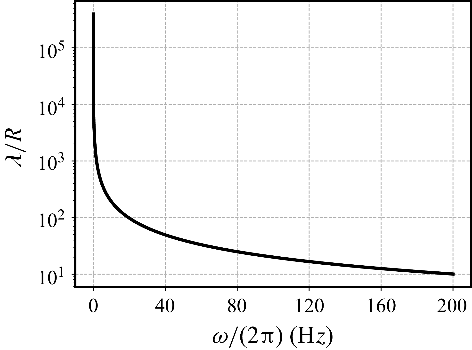
Wavelength
 $ \lambda$
normalised by the local radius at
 $z=l/2$
versus frequency
 $ \omega$
. Parameters from the baseline case are used except
 $\tau =0$
.

Since the wavelength is related to the angular frequency by  , the wave frequency must remain sufficiently low to satisfy the long-wave assumption. To assess the validity of this approximation, the wavelength is plotted as a function of frequency in figure 9, using the parameters introduced in § 4. As expected,
 $\lambda$
decreases monotonically with increasing
 $\omega$
. Notably, even at 200 Hz, the wavelength remains roughly 10 times greater than the local radius, confirming that the long-wave assumption holds at least up to this frequency.