


1. Introduction
Understanding phase transitions is a central task in discrete probability and statistical physics. One of the most basic questions about a phase transition is whether it is continuous or first-order. That is, when a quantity undergoes a phase transition, does it vary continuously as a parameter is varied, or does it take a discontinuous jump at criticality? This question is often difficult. For example, the phase transition for the probability that the origin belongs to an infinite component in bond percolation on the lattice is thought to be continuous, but it remains unproven in dimensions
 $3,\ldots,10$
[Reference Fitzner and van der Hofstad10, Reference Hara and Slade13].
This paper investigates phase transitions on Galton–Watson trees for events satisfying certain recursive properties. This setting is inspired by two examples. Let
 $\mathcal{T}_1$
be the set of infinite rooted trees and let
 $\mathcal{T}_2$
be the set of trees containing an infinite binary tree starting from the root. Let
 $T_\lambda$
be a Galton–Watson tree with child distribution
 $\textrm{Poi}(\lambda)$
. The event
 $\{T_\lambda\in\mathcal{T}_1\}$
has probability 0 for
 $\lambda<1$
. It undergoes a continuous phase transition at
 $\lambda=1$
, with its probability rising from 0 as
 $\lambda$
increases above 1. On the other hand, the event
 $\{T_\lambda\in\mathcal{T}_2\}$
has probability 0 for
 $\lambda<\lambda_{\textrm{crit}}\approx 3.35$
. Its probability jumps to approximately 0.535 at
 $\lambda=\lambda_{\textrm{crit}}$
and increases continuously after that. See [Reference Johnson, Podder and Skerman14, Example 5.5] for a detailed treatment of this example; see [Reference Pittel, Spencer and Wormald18] for this example in the context of random graphs; and see [Reference Dekking6] for an earlier analysis of
 $\mathcal{T}_2$
and proof that the phase transition is discontinuous for a different family of child distributions.
The sets
 $\mathcal{T}_1$
and
 $\mathcal{T}_2$
both satisfy recursive properties. A tree is in
 $\mathcal{T}_1$
if and only if the root has at least one child that initiates a tree in
 $\mathcal{T}_1$
. Similarly, a tree is in
 $\mathcal{T}_2$
if and only if the root has at least two children that initiate trees in
 $\mathcal{T}_2$
. Why does
 $\mathcal{T}_1$
have a continuous phase transition while
 $\mathcal{T}_2$
does not? The goal of this paper is to answer this question, and more generally to explain the connection between the recursive property that an event satisfies and the phase transition that the event undergoes. It will take some work to state our results, but let us start with an informal account.
First, the event
 $\mathcal{T}_2$
will never have a continuous phase transition under any family of child distributions. For this event, we say that the threshold function
 $h(\ell)$
is identically 2, meaning that regardless of the count
 $\ell$
of children of the root of the tree, the event
 $\mathcal{T}_2$
holds if and only if at least two of the children initiate a tree in
 $\mathcal{T}_2$
. For
 $\mathcal{T}_1$
, the associated threshold function is identically 1. (We will define threshold functions more formally in Section 1.2.) Theorems 1.2 and 1.5 give a criterion for whether a continuous phase transition occurs at a child distribution
 $\chi$
given the threshold function h of the event. In particular, a continuous phase transition can occur at a child distribution
 $\chi$
only if
 \begin{align*} \sum_{\text{$\ell\colon h(\ell)=1$}}\chi(\ell)\ell=1.\end{align*}
This is satisfied for
 $\mathcal{T}_1$
whenever the child distribution has mean 1, but it is never satisfied for
 $\mathcal{T}_2$
.
The criterion given by Theorems 1.2 and 1.5 for when continuous phase transitions occur is one of the two main results of the paper, although it is not particularly difficult to show using results from [Reference Johnson, Podder and Skerman14]. The bulk of the work in this paper is to prove the other main result, Theorem 1.8, which runs in the opposite direction as our examples so far. Suppose we start with a recursive property, without any example of a set of trees satisfying the property. Proposition 1.1 and Theorems 1.2 and 1.5 work together to prove that there exists some set of trees satisfying the recursive property, and that at a certain Galton–Watson measure the probability of this set of trees undergoes a continuous phase transition. But these results do not describe this set of trees. Theorem 1.8 characterises this set in many circumstances.
To state our results, we must establish what exactly we mean when we say a set of trees satisfies a recursive property. A more general version of this framework is given in [Reference Johnson, Podder and Skerman14]. Our terminology here is consistent with this more general version, though we will only introduce what we need here.
1.1. General notation
For a probability distribution
 $\chi$
on the non-negative integers, we will abbreviate quantities like
 $\chi(\{n\})$
to
 $\chi(n)$
. We use
 $\textrm{GW}_{{\chi}}$
to denote the Galton–Watson measure with child distribution
 $\chi$
on the space of rooted trees. Let
 $n_t(v)$
denote the number of children of a vertex v in a rooted tree t. We refer to the subtrees originated by the children of the root of a tree as its root-child subtrees. We abuse notation slightly and use expressions like
 $\textrm{Bin}(n,p)$
and
 $\textrm{Poi}(\mu)$
to denote both a distribution and a random variable with that distribution, in statements like
 $\mathbb{P}[\textrm{Bin}(n,p)=k] = \binom{n}{k}p^k(1-p)^{n-k}$
. For a random variable N on the non-negative integers,
 $\textrm{Bin}(N,p)$
denotes a random variable whose law is the mixture of binomial distributions governed by the law of N (i.e.
 $\mathbb{P}[\textrm{Bin}(N,p)=k]=\sum_{n=0}^{\infty}\mathbb{P}[N=n]\mathbb{P}[\textrm{Bin}(n,p)=k]$
). We denote the falling factorial
 $n(n-1)\cdots (n-k+1)$
by the notation
 $(n)_k$
. Let
 $\mathbb{N}=\{0,1,2,\ldots\}$
.
1.2. Encoding recursive properties
As we hinted earlier, we will describe recursive properties by giving a threshold function h. For a tree whose root has
 $\ell\geq 0$
children, we think of
 $h(\ell)$
as the minimum number of its root-child subtrees with a given property to force the tree itself to have that property. If an event is consistent with the recursive property encoded by h, we call it an interpretation of h. To formalise this, for a rooted tree t let
 $\ell(t)$
denote the number of children of the root of t. For a set of trees
 $\mathcal{T}$
, let
 $c(t,\mathcal{T})$
denote the number of root-child subtrees of t that are elements of
 $\mathcal{T}$
. For a given child distribution
 $\chi$
and threshold function h, we say that a
 $\textrm{GW}_{{\chi}}$
-measurable set of trees
 $\mathcal{T}$
is an interpretation of
 $(\chi,h)$
if
 \begin{align} t\in\mathcal{T} \iff c(t,\mathcal{T})\geq h\bigl(\ell(t)\bigr) \qquad {\rm{for\,G}}{{\rm{W}}_\chi }{\rm{ - a}}.{\rm{e}}.\;{\rm{rooted\,tree\,}}t.\end{align}
For example, the set
 $\mathcal{T}_1$
of infinite trees is an interpretation of
 $(\chi,h)$
where
 $h(\ell)\equiv 1$
and the set
 $\mathcal{T}_2$
of trees containing an infinite binary tree starting from the root is an interpretation of
 $(\chi,h)$
where
 $h(\ell)\equiv 2$
. In both of these cases, (1) holds for all trees t, not just for
 $\textrm{GW}_{{\chi}}$
-a.e. tree t, which renders
 $\chi$
irrelevant. In such cases we will often call our event an interpretation of h, omitting reference to the child distribution. (Excluding negligible sets in the definition is required for some of the results in [Reference Johnson, Podder and Skerman14].)
For context, let us describe how these recursive properties fit into the broader class considered in [Reference Johnson, Podder and Skerman14]. Suppose that the root of t has
 $\ell$
children, and that
 $n_1$
originate trees with some property while
 $n_0$
of them do not. Suppose that the counts
 $n_0$
and
 $n_1$
determine whether t itself has the property, and let the map
 $A\colon\mathbb{N}^2\to\{0,1\}$
specify this, with
 $A(n_0,n_1)=1$
when t has the the property and
 $A(n_0,n_1)=0$
when it does not. In [Reference Johnson, Podder and Skerman14], this map A is called a tree automaton, and an event consistent with the recursive property described by the automaton is called an interpretation of it. Recursive properties defined by a threshold function h correspond to automata of the form
 $A(n_0,n_1)=\textbf{1}\{n_1\geq h(n_0+n_1)\}$
, which in [Reference Johnson, Podder and Skerman14] are called monotone automata. We restrict ourselves to such automata because we have stronger results for them, primarily because the Margulis–Russo lemma provides a powerful tool for their analysis (see [Reference Johnson, Podder and Skerman14, Section 5.1]).
The tree automata described above are called two-state, in that each tree has one of two possible states (having the property or not having the property) and the state of a tree is determined by the states of its root-child subtrees. In [Reference Johnson, Podder and Skerman14], automata are considered with more than two states, which again increases the complexity of the theory.
In this paper, we will often impose the additional condition that
 $h(\ell)$
is (nonstrictly) increasing in
 $\ell$
. This is also a form of monotonicity for the recursive property; it amounts to declaring that if a tree t has the property, then it still has it after attaching an additional subtree to the root.
1.3. Fixed points
As we will soon see, the probability of an interpretation under the Galton–Watson measure satisfies a fixed-point equation determined by the threshold function and child distribution. The classical example is the probability that a Galton–Watson survives (i.e. probability of the set
 $\mathcal{T}_1$
discussed in Section 1.2). Taking
 $T_\lambda\sim\textrm{GW}_{{\textrm{Poi}(\lambda)}}$
, let
 $x= \mathbb{P}[T_\lambda\in\mathcal{T}_1]$
. Since
 $T_\lambda\in\mathcal{T}_1$
if and only if at least one of the root-child subtrees of
 $T_\lambda$
is in
 $\mathcal{T}_1$
, and each of the
 $\textrm{Poi}(\lambda)$
root-child subtrees has probability x of being in
 $\mathcal{T}_1$
,
 \begin{align} x = \mathbb{P}[\textrm{Poi}(\lambda x)\geq 1] = 1 - e^{-\lambda x}\end{align}
by Poisson thinning. This equation has two solutions when
 $\lambda>1$
, and in this case x turns out to be the larger of the two (the smaller is 0).
To give the fixed-point equation in a general case, we define the automaton distribution map
 $\Psi(x)$
for a given child distribution
 $\chi$
and threshold function h. (The terminology automaton distribution map comes from a generalisation in [Reference Johnson, Podder and Skerman14] that maps distributions to distributions.) With
 $L\sim\chi$
, we define
 \begin{align} \Psi(x) = \mathbb{P}[ \textrm{Bin}(L,x) \geq h(L) ] = \sum_{\ell=0}^{\infty}\chi(\ell)\mathbb{P}\bigl[\textrm{Bin}(\ell,x)\geq h(\ell)\bigr].\end{align}
In words,
 $\Psi(x)$
is the probability that at least h(L) out of L root-child subtrees of a Galton–Watson tree have some property that holds for each of them with probability x.
Observe that the right-hand side of (2) is the automaton distribution map for
 $\chi=\textrm{Poi}(\lambda)$
and
 $h(\ell)\equiv 1$
. Thus (2) is the statement that the probability of the interpretation
 $\mathcal{T}_1$
under
 $\textrm{GW}_{{\chi}}$
is a fixed point of the automaton distribution map. In fact, it holds in general that for any child distribution
 $\chi$
and threshold function h, the probability of an interpretation
 $\mathcal{T}$
of
 $(\chi,h)$
is a fixed point of its automaton distribution map: Let
 $T\sim\textrm{GW}_{{\chi}}$
and let
 $x=\mathbb{P}[T\in\mathcal{T}]$
. Conditional on the number of children of the root of T, each root-child subtree in T lies in
 $\mathcal{T}$
independently with probability x, since the root-child subtrees are themselves independently sampled from
 $\textrm{GW}_{{\chi}}$
. Because
 $\mathcal{T}$
is an interpretation of A, the tree’s membership in
 $\mathcal{T}$
is determined from its root-child subtrees’ membership in
 $\mathcal{T}$
according to h. Thus
 $\Psi(x)=\mathbb{P}[T\in\mathcal{T}]=x$
.
We are interested in circumstances in which the automaton distribution maps have 0 as a fixed point, since we are investigating phase transitions emerging from 0. Thus we typically require the threshold function h to satisfy
 $h(\ell)\geq 1$
for all
 $\ell\geq 0$
. (Strictly speaking, to make 0 a fixed point we only need
 $h(\ell)\geq 1$
for
 $\ell$
in the support of the child distribution, but the value of
 $h(\ell)$
for
 $\ell$
outside of this support is irrelevant anyhow.)
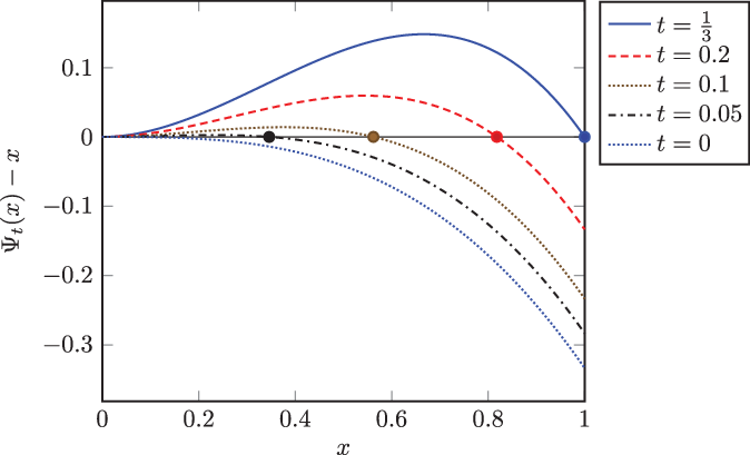
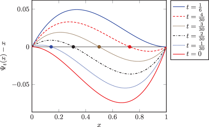
Let
 $\chi_t$
be the probability measure placing the vector of probabilities
 $\bigl(\frac13-t,\,0,\,\frac12,\,\frac16+t\bigr)$
on values
 $0,\,1,\,2,\,3$
. Let
 $h(0)=h(1)=h(2)=1$
and
 $h(3)=2$
. The graphs above depict
 $\Psi_t(x)$
, the automaton distribution map of
 $(\chi_t,h)$
. The recursive tree system
 $(\chi_t,h)$
is critical at
 $t=0$
in the sense of Definition 1.4. As t increases, a single interpretable fixed point emerges and increases to 1 as t rises to
 $1/3$
.

1.4. Results
Fix a threshold function h, and let
 $\Psi_{\chi}$
be the automaton distribution map for
 $(\chi,h)$
. Our aim is to understand the circumstances in which
 $\chi$
is critical, in the sense that there is an event satisfying the recursive property encoded by h whose probability emerges from 0 as
 $\chi$
is perturbed (we will make this definition precise in Definition 1.4). Since an event satisfying the recursive property has probability given by a fixed point of
 $\Psi_\chi$
, a new fixed point must emerge from 0 as
 $\chi$
is perturbed. Based on the idea that
 $\Psi_\chi$
changes continuously in
 $\chi$
, intuition suggests that
 $\Psi'_\chi(0)=1$
is necessary in order to have a fixed point emerge from 0 as
 $\chi$
is varied (see Figure 1 for an example of a fixed point emerging). This thought is on the right track, but it raises some questions:
-
a. Suppose that
 $\chi$
can be perturbed so that a fixed point of
$\Psi_\chi$
emerges from 0. Is it always the case that this fixed point has an interpretation? That is, is there an event satisfying the recursive property whose probability is given by the fixed point (and which therefore has a phase transition)?
-
b. Can we characterise the critical child measures
$\chi$
in a more direct way than stating properties of
$\Psi_\chi$
? -
c. Suppose that
$\Psi_\chi$
has a fixed point emerging from 0 as
$\chi$
is perturbed, and we can determine that indeed
$\chi$
is critical, i.e. that there exists an interpretation associated with this fixed point undergoing a phase transition. Can we state what the interpretation is in any satisfying way?


Before we address these questions and present our results, let us recall and define some notation. For a given child distribution
 $\chi$
, we will be posing questions about the interpretations of
 $(\chi,h)$
, as defined in Section 1.2. We call
 $(\chi,h)$
a recursive tree system, and we take as part of the definition that
 $h(\ell)\geq 1$
for all
 $\ell\geq 0$
. As we explained in Section 1.3, any interpretation of
 $(\chi,h)$
has
 $\textrm{GW}_{{\chi}}$
-measure satisfying the fixed-point equation
 $\Psi(x)=x$
, where
 $\Psi$
is the automaton distribution map of
 $(\chi,h)$
. If
 $\mathcal{T}$
is an interpretation of
 $(\chi,h)$
with
 $\textrm{GW}_{{\chi}}(\mathcal{T})=x_0$
, then we say that
 $\mathcal{T}$
is the interpretation associated with the fixed point
 $x_0$
(we write the interpretation rather than an interpretation because we show in Proposition 1.1 that a given fixed point can have at most one interpretation). We refer to the fixed points of
 $\Psi$
as the fixed points of
 $(\chi,h)$
. For a system
 $(\chi,h)$
, we define its kth tier as the set of values
 $\ell\geq 1$
in the support of
 $\chi$
with
 $h(\ell)=k$
. That is, tier k for
 $(\chi,h)$
is defined as
 \begin{align} \textrm{tier}(k)=\textrm{tier}_{\chi,h}(k)=\bigl\{ \ell\geq 1\colon \text{$h(\ell)=k$ and $\chi(\ell)>0$} \bigr\}.\end{align}
Question a is resolved by the following criterion for when a fixed point of
 $(\chi,h)$
admits an interpretation:
Proposition 1.1. Let
 $\chi$
have finite expectation and more than one point of support, let
 $\Psi$
be the automaton distribution map of the recursive tree system
 $(\chi,h)$
, and let
 $0<x_0<1$
be a fixed point of
 $(\chi,h)$
. There exists an interpretation of
 $(\chi,h)$
associated with
 $x_0$
if and only if
 $\Psi'(x_0)\leq 1$
. When an interpretation of
 $x_0$
exists, it is unique up to
 $\textrm{GW}_{{\chi}}$
-negligible sets.
We give a proof in Section 2, though it just amounts to tying together results from [Reference Johnson, Podder and Skerman14]. Proposition 1.1 does not address the case of
 $x_0=0$
or
 $x_0=1$
because such fixed points have trivial interpretations associated with them, namely the empty set in the case of 0 and the set of all rooted trees in the case of 1.
To address question b, we give a formula for the derivatives of
 $\Psi$
at zero in terms of
 $\chi$
. The notation
 $(\ell)_m$
in (5) and (6) denotes the falling factorial
 $\ell(\ell-1)\cdots (\ell-m+1)$
.
Theorem 1.2. Let
 $\chi$
be a child distribution with finite mth moment, and let
 $\Psi$
be the automaton distribution map of the recursive tree system
 $(\chi,h)$
. Then for
 $m\geq 1$
,
 \begin{align} \Psi^{(m)}(0) &= \sum_{\ell=m}^{\infty}(-1)^{m+h(\ell)}\binom{m-1}{h(\ell)-1}\chi(\ell)(\ell)_m,\end{align}
 \begin{align} &= \sum_{j=1}^m (-1)^{m+j}\binom{m-1}{j-1}\sum_{\ell\in\textrm{tier}(j)} \chi(\ell)(\ell)_m. \end{align}
We highlight the
 $m=1,2$
cases of this theorem:
 \begin{align} \Psi'(0) &= \sum_{\ell\in\textrm{tier}(1)} \chi(\ell)\ell,\end{align}
 \begin{align} \Psi''(0) &= \sum_{\ell\in\textrm{tier}(2)} \chi(\ell)\ell(\ell-1) -\sum_{\ell\in\textrm{tier}(1)} \chi(\ell)\ell(\ell-1) .\end{align}
It follows from Theorem 1.2 that the value of
 $\Psi^{(m)}(0)$
depends only on the mass that
 $\chi$
places on the first m tiers. We state this formally since we will often use it:
Corollary 1.3. Assume that
 $\chi$
and
 $\widetilde\chi$
have finite mth moments. Let
 $\Psi$
and
 $\widetilde\Psi$
be the automaton distribution maps of the recursive tree systems
 $(\chi,h)$
and
 $(\widetilde\chi,h)$
, respectively. If
 $\chi(\ell)=\widetilde\chi(\ell)$
whenever
 $h(\ell)\leq m$
, then
 $\Psi^{(m)}(0)=\widetilde\Psi^{(m)}(0)$
.
Now, we can relate conditions on the derivatives of
 $\Psi$
at 0 back to the child distribution. With this in mind, we will state our criteria for where continuous phase transitions occur. Let
 ${\Pi_{\infty}}$
denote the space of probability measures on the non-negative integers with all moments finite. On
 ${\Pi_{\infty}}$
, for any
 $n\geq 0$
we can define a metric
 \begin{align*} d_n(\chi_1,\chi_2) &= \sum_{k=1 }^{\infty} k^n\left\lvert{\chi_1(k)-\chi_2(k)}\right\rvert.\end{align*}
We topologise
 ${\Pi_{\infty}}$
by declaring that
 $\chi_n\to\chi$
if
 $d_n(\chi_n,\chi)\to 0$
for all
 $n\geq 0$
. We work in this space to avoid pathologies; see Remark 1.7 for more details.
Definition 1.4. For a recursive tree system
 $(\chi,h)$
with
 $\chi\in{\Pi_{\infty}}$
, we say that
 $(\chi, h)$
is critical if for any
 $\epsilon>0$
, all neighbourhoods of
 $\chi$
in
 ${\Pi_{\infty}}$
contain a measure
 $\pi$
such that there is an interpretation
 $\mathcal{T}$
of
 $(\pi,h)$
satisfying
 $0<\textrm{GW}_{{\pi}}(\mathcal{T})<\epsilon$
. Equivalently,
 $(\chi,h)$
is critical if there exists a sequence
 $\chi_n\in{\Pi_{\infty}}$
converging to
 $\chi$
such that
 $(\chi_n,h)$
has an interpretation
 $\mathcal{T}_n$
with
 $\textrm{GW}_{{\chi_n}}(\mathcal{T}_n)\searrow 0$
.
Theorem 1.5 Let
 $\chi\in{\Pi_{\infty}}$
have more than one point of support. The recursive tree system
 $(\chi,h)$
with automaton distribution map
 $\Psi$
is critical if and only if
 $\Psi'(0)=1$
and
 $\Psi''(0)\leq 0$
.
Remark 1.6. One might object that to correctly capture the idea of a phase transition, we should insist on a single interpretation
 $\mathcal{T}$
satisfying
 $\textrm{GW}_{{\chi_n}}(\mathcal{T})\searrow 0$
, rather than a sequence of interpretations
 $\mathcal{T}_n$
with
 $\textrm{GW}_{{\chi_n}}(\mathcal{T}_n)\searrow 0$
. For example, suppose
 $h(\ell)\equiv 1$
,
 $\chi=\textrm{Poi}(1)$
, and
 $\chi_n=\textrm{Poi}(1+1/n)$
. Then for the set of infinite trees
 $\mathcal{T}_1$
, we have
 $\textrm{GW}_{{\chi_n}}(\mathcal{T}_1)\searrow 0$
. In fact, this more stringent requirement is equivalent to our original one, as we now show. First, we claim that for different child distributions
 $\chi$
and
 $\chi'$
, the measures
 $\textrm{GW}_{{\chi}}$
and
 $\textrm{GW}_{{\chi'}}$
restricted to infinite trees are mutually singular. To see this, observe that for
 $\textrm{GW}_{{\chi}}$
-a.e. infinite tree t, the empirical distribution of the numbers of children of the vertices at level n of the tree converges to
 $\chi$
. Hence the supports of
 $\textrm{GW}_{{\chi}}$
and
 $\textrm{GW}_{{\chi'}}$
on infinite trees are disjoint.
Next, any interpretation contains only infinite trees by our requirement that
 $h(\ell)\geq 1$
. To see this, let
 $\mathcal{T}$
be an interpretation, and observe that a single-vertex tree is not a member of
 $\mathcal{T}$
since 0 of its 0 root-child vertices are in
 $\mathcal{T}$
, and
 $h(0)\geq 1$
. Then since single-vertex trees are not members of
 $\mathcal{T}$
, no height-1 tree can be in
 $\mathcal{T}$
, and hence no height-2 tree can be in
 $\mathcal{T}$
, and so on.
Thus, if we have a sequence of interpretations
 $\mathcal{T}_n$
of
 $(\chi_n,h)$
satisfying
 $\textrm{GW}_{{\chi_n}}(\mathcal{T}_n)\searrow 0$
, we can stitch them together into a single interpretation
 $\mathcal{T}$
defined to be equal to
 $\mathcal{T}_n$
on the support of
 $\textrm{GW}_{{\chi_n}}$
. However, we will see in Theorem 1.8 that for a large class of phase transitions, we can define a single interpretation
 $\mathcal{T}$
in a more satisfying way so that
 $\textrm{GW}_{{\chi_n}}(\mathcal{T})\searrow 0$
.
Remark 1.7 The details of the topology on
 ${\Pi_{\infty}}$
are not particularly important to this paper, but let us define it in more detail and explain what goes wrong with a looser sense of convergence. To make it so that
 $\chi_n\to\chi$
if and only if
 $d_n(\chi_n,\chi)\to 0$
for all
 $n\geq 0$
, consider the product space
 $\prod_{n=0}^{\infty}{\Pi_{\infty}}$
where the nth copy of
 ${\Pi_{\infty}}$
is taken as the metric space
 $({\Pi_{\infty}},d_n)$
. Now consider the map
 $\iota\colon {\Pi_{\infty}}\to\prod_{n=0}^{\infty}{\Pi_{\infty}}$
given by
 $\iota(\chi)=(\chi,\chi,\ldots)$
. We assign
 ${\Pi_{\infty}}$
the topology induced by
 $\iota$
, i.e. the one formed by pullbacks of open sets in the product space.
Problems arise if we use a coarser topology on
 ${\Pi_{\infty}}$
. For example, suppose we use the metric
 $d_0$
, which in this space metrises the topology of convergence in law. Now, for the threshold function
 $h(\ell)\equiv 1$
, even the measure
 $\delta_0$
is critical. Indeed, define
 \begin{align*} \chi_n=(1-2/n)\delta_0 + (2/n)\delta_n. \end{align*}
Then
 $d_0(\chi_n,\chi)\to 0$
and
 $\textrm{GW}_{{\chi_n}}(\mathcal{T}_1)\searrow 0$
, where
 $\mathcal{T}_1$
is the set of infinite rooted trees.
Finally, we address question c and try to describe the event undergoing the continuous phase transition. Our result, Theorem 1.8, characterises the interpretation associated with the smallest non-zero fixed point when its automaton distribution map
 $\Psi(x)$
satisfies
 $\Psi(x)>x$
on some interval
 $(0,\epsilon)$
for
 $\epsilon>0$
. This means that the result describes the event undergoing a phase transition so long as the graph of the automaton distribution map rises above the line
 $y=x$
as the phase transition occurs. This occurs in the phase transitions illustrated in Figures 1 and 2, but not in the phase transition shown in Figure 3. We also mention that Theorem 1.8 requires
 $h(\ell)$
to be increasing.
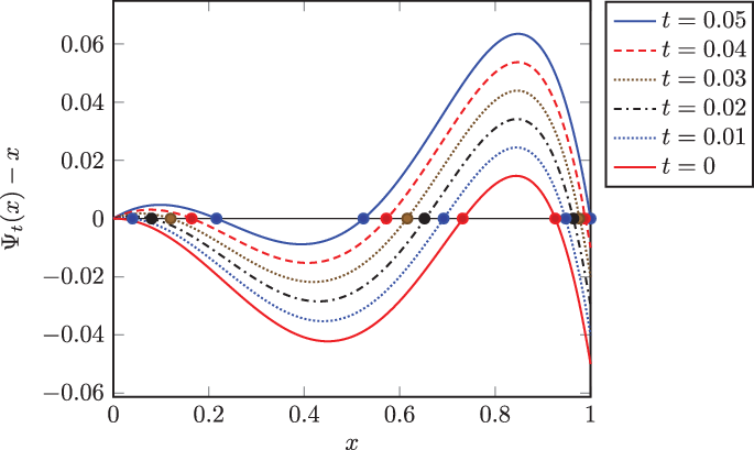
Graphs of
 $\Psi_t(x)-x$
, where
 $\Psi_t$
is the automaton distribution map of
 $(\chi_t,h)$
with
 $\chi_t = \bigl(\frac{1}{20} - t\bigr)\delta_0 + \bigl(\frac12+t\bigr)\delta_2 + \frac{9}{20}\delta_5$
, and
 $h(0)=h(2)=1$
and
 $h(5)=4$
. The system
 $(\chi_t,h)$
is critical at
 $t=0$
in the sense of Definition 1.4, and we can see a fixed point emerging from 0 as t increases. Because
 $\Psi_t(x)\geq x$
in a neighbourhood of 0 for
 $t>0$
, the interpretation associated with this fixed point is described in Theorem 1.8. See Example 1.8 for more details.

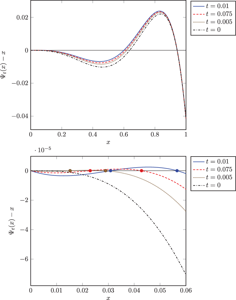
Graphs of
 $\Psi_t(x)-x$
illustrating a continuous phase transition not satisfying the conditions of Theorem 1.8. Here
 $\Psi_t$
is the automaton distribution map for
 $(\chi_t,h)$
where
 $\chi_t = \frac{1}{24}\delta_0 + \bigl(\frac12 - 3t^2\bigr)\delta_2 + \bigl(\frac16 + t\bigr)\delta_3 + \bigl(\frac{7}{24}+3t^2-t\bigr)\delta_6$
, and
 $h(0)=h(2)=1$
,
 $h(3)=2$
, and
 $h(6)=5$
. The top plot is our standard view of
 $\Psi_t(x)-x$
as in Figures 1 and 2. In the bottom plot, we zoom in around
 $x=0$
and see that two fixed points emerge from zero as t increases. By Proposition 1.1, the first fixed point for each system has no interpretation but the second one does. But we cannot apply Theorem 1.8 to characterise this interpretation. See Section 5 for further discussion.

The characterisation of the interpretation depends on the behaviour of the automaton distribution map near 0. We define some terminology about this now. For
 $m\geq 1$
, we say that the recursive tree system
 $(\chi,h)$
is m-concordant if the first m derivatives of
 $\Psi$
at 0 match those of the function x. That is,
 $(\chi,h)$
is m-concordant if
 $\Psi'(0)=1$
and
 $\Psi^{(k)}(0)=0$
for
 $2\leq k\leq m$
. For
 $m\geq 2$
, we say that
 $(\chi,h)$
is m-subcordant (resp. m-supercordant) if it is
 $(m-1)$
-concordant and
 $\Psi^{(m)}(0)<0$
(resp.
 $\Psi^{(m)}(0)>0$
). We say that
 $(\chi,h)$
is 1-concordant, 1-subcordant, or 1-supercordant if
 $\Psi'(0)=1$
,
 $\Psi'(0)<1$
, or
 $\Psi'(0)>1$
, respectively. When h is clear from context, we will abuse notation and refer to
 $\chi$
itself as being m-concordant, m-subcordant, or m-supercordant. Note that assuming smoothness of
 $\Psi$
(which holds for
 $\chi\in{\Pi_{\infty}}$
by Lemma 2.3), if
 $\Psi(x)> x$
holds on some interval
 $(0,\epsilon)$
, then
 $(\chi,h)$
is m-supercordant for some
 $m\geq 1$
.
Finally, we define the notion of an admissible subtree. We say that a subtree s of a rooted tree t is admissible with respect to a threshold function h if s contains the root of t and
 $n_s(v)\geq h(n_t(v))$
for all vertices
 $v\in s$
. We can think of an admissible subtree as a sort of witness to an interpretation. For example, consider
 $h(\ell)\equiv 1$
, the threshold function encoding a property that holds for a tree if and only if it holds for at least one of the tree’s root-child subtrees. As we mentioned earlier, this recursive tree system has two fixed points when
 $\chi$
has mean greater than 1, and the interpretation of the non-zero fixed point is survival of the Galton–Watson tree. A subtree S of the Galton–Watson tree T is admissible if and only if S has no leaves (i.e.
 $n_S(v)\geq 1$
for all
 $v\in S$
). An admissible subtree thus serves as a witness to the Galton–Watson tree being infinite. Indeed, the event of T being infinite could equally well be described as T having an admissible subtree (see Proposition 1.9 for a generalisation).
Theorem 1.8 Let
 $\chi\in{\Pi_{\infty}}$
have more than one point of support. Consider the recursive tree system
 $(\chi,h)$
with automaton distribution map
 $\Psi$
, and assume that
 $h(\ell)$
is increasing in
 $\ell$
. Suppose that
 $(\chi,h)$
is m-supercordant, and let
 $x_0$
be the smallest non-zero fixed point of
 $\Psi$
. Then
 $x_0$
is interpretable, and its associated interpretation is the event that
 $T\sim\textrm{GW}_{{\chi}}$
contains an admissible subtree S in which all but finitely many vertices v satisfy
 $n_S(v)\leq m$
.
Though it falls outside this narrative of understanding phase transitions, we mention that in all cases, the highest fixed point of a recursive tree system has a similar characterisation:
Proposition 1.9 Let
 $\chi\in{\Pi_{\infty}}$
have more than one point of support. Consider the recursive tree system
 $(\chi,h)$
with automaton distribution map
 $\Psi$
. Let
 $x_1$
be the largest fixed point of
 $\Psi$
. Then
 $x_1$
is interpretable, and its associated interpretation is the event that
 $T\sim\textrm{GW}_{{\chi}}$
contains an admissible subtree.
We close the section with an example of a family of systems
 $(\chi_t,h)$
undergoing a continuous phase transition, as shown in Figure 2.
Example 1.10 Define
 $\chi_t$
and h by
 \begin{align*} \chi_t(\ell)=\begin{cases} 1/20 - t & \text{for $\ell=0$,}\\[4pt]
1/2 + t & \text{for $\ell=2$,}\\[4pt]
9/20 & \text{for $\ell=5$,}\\ \end{cases}\qquad\qquad \text{and} \qquad\qquad h(\ell)=\begin{cases} 1 & \text{for $\ell=0$,}\\[4pt]
1 & \text{for $\ell=2$,}\\[4pt]
4 & \text{for $\ell=5$,} \end{cases} \end{align*}
and let
 $\Psi_t$
be the automaton distribution map of the recursive tree system
 $(\chi_t,h)$
. By Theorem 1.2,
 \begin{align*} \Psi'_t(0) &= 2\chi_t(2) = 1 + 2t,\\[4pt] \Psi''_t(0) &= -2\chi_t(2) = -1-2t. \end{align*}
The system
 $(\chi_0,h)$
is critical by Theorem 1.5, since
 $\Psi'_0(0)=1$
and
 $\Psi''_0(0)=-1$
. For
 $t>0$
, the system is 1-supercordant (i.e.
 $\Psi'_t(0)>1$
).
In Figure 2, we show the graphs of
 $\Psi_t(x)-x$
, so that fixed points of
 $\Psi_t$
appear as roots. At
 $t=0$
, the system has two non-zero fixed points, at
 $x\approx 0.73$
and
 $x\approx 0.93$
. As t grows, a fixed point
 $x_0(t)$
emerges from 0. We have
 $\Psi'_t(x_0(t))<1$
, evident from the graph of
 $\Psi_t(x)-x$
where
 $x_0$
is a down-crossing root. By Proposition 1.1, the fixed point
 $x_0(t)$
is interpretable. By Theorem1.8, the interpretation of
 $(\chi_t,h)$
associated with
 $x_0(t)$
is the event
 $\mathcal{T}_0$
that
 $T\sim\textrm{GW}_{{\chi}}$
has an admissible subtree S in which all but finitely many vertices
 $v\in S$
satisfy
 $n_S(v)\leq 1$
. Since
 $h(\ell)>0$
for all
 $\ell\geq 0$
, an admissible subtree has no leaves, and thus all but finitely many vertices have
 $n_S(v)=1$
.
Recall that
 $S\subseteq T$
is admissible if it contains the root of T and for each v in S, we have
 $n_S(v)\geq h(n_T(v))$
. In this case, if a vertex v has 5 children in T, it can only be in S if at least 4 of those children are also in S; if v has 2 children in T, it can only be in S if at least one of those children is in S; and if it has no children in T, it cannot be in S. Thus on the event
 $\mathcal{T}_0$
, the tree T contains an admissible subtree where all but finitely many vertices have 2 children in T.
We can see directly that
 $\textrm{GW}_{{\chi_0}}(\mathcal{T}_0)=0$
by observing that the subtree of
 $T\sim\textrm{GW}_{{\chi_0}}$
consisting only of the vertices with 2 or fewer children forms a critical Galton–Watson tree (its child distribution is
 $\frac12\delta_0+\frac12\delta_2$
). Thus it has no chance of being infinite. Consequently, for any vertex v in T, there is no chance that T(v) contains an admissible subtree consisting of only vertices with 2 children in T.
Viewing the graph in Figure 2, we observe that
 $\Psi_t$
has derivative greater than 1 at its middle fixed point, which means that it has no interpretation by Proposition 1.1. The largest fixed point has the interpretation that
 $T\sim\textrm{GW}_{{\chi_t}}$
contains an admissible subtree, by Proposition 1.9.
1.5. Related work
A finite random structure like a random graph will not typically experience a true phase transition. The analogous concept in this area is a sharp threshold for some property, meaning that the property holds with probability that transitions from 0 to 1 in a parameter window that tends to 0 as the system grows. The motivating phase transitions of this paper—the continuous phase transition for survival and the first-order transition for existence of a binary subtree in a Galton–Watson tree—have analogues for Erdös–Rényi random graphs in this sense: the existence of giant component [Reference Alon and Spencer2, Chapter 11], and the existence of a 3-core [Reference Pittel, Spencer and Wormald18, Reference Riordan19]. The first of these examples is essentially a continuous phase transition while the second is essentially first-order. For example, when one reaches the threshold for a 3-core to exist, it immediately makes up a positive linear fraction of the graph’s vertices. These examples have been studied extensively, though not in the sort of general framework considered in this paper.
As for more general studies of phase transitions and sharp thresholds, in finite systems, there is a line of inquiry centred on giving conditions for a property to have a sharp threshold [Reference Friedgut and Kalai8, Reference Friedgut9, Reference Łuczak and Spencer15, Reference Shelah and Spencer21]. Many of these results use the theory of Boolean functions and the Margulis–Russo formula (see [Reference Garban and Steif11] for background), also used in this paper for the proof of Proposition 1.1 via [Reference Johnson, Podder and Skerman14]. These results on sharp thresholds for finite random structures have been applied in impressive ways to prove results on phase transitions for infinite systems [Reference Bollobás and Riordan4, Reference Duminil-Copin5]. There is also considerable nonrigorous literature by physicists on distinguishing between continuous and first-order phase transitions (see, e.g [Reference Boccaletti, Almendral, Guan, Leyva, Liu, Sendia-Nadal, Wang and Zou3, Reference Encinas, Harunari, de Oliveira and Fiore7]).
For Galton–Watson trees specifically, Podder and Spencer investigate probabilities of events that can be described in first-order logic (no connection to first-order phase transitions) in [Reference Podder and Spencer16, Reference Podder and Spencer17]. These events have the same sort of recursive description as the events considered here, generally with more than two states. But their fundamental result [Reference Podder and Spencer17, Theorem 1.2] is that these events never undergo phase transitions at all. In [Reference Holroyd and Martin12], Holroyd and Martin consider various two-player games whose moves are modelled by directed steps on a Galton–Watson tree. They investigate events of a player winning the game in various senses, which have a similar recursive nature as the events considered here, and they give results about the continuity or discontinuity of phase transitions for these events [Reference Holroyd and Martin12, Theorem 5].
1.6. Sketches of proofs
The proofs of Theorems 1.2 and 1.5 are fairly straightforward. For Theorem 1.2, we express
 $\Psi(x)$
as a sum of polynomials and carry out combinatorial calculations to compute their derivatives. Proving Theorem 1.5 is just a matter of Taylor approximation of
 $\Psi(x)$
near
 $x=0$
combined with Proposition 1.1, our interpretability criterion from [Reference Johnson, Podder and Skerman14]. Section 2 is devoted to these two proofs.
The proof of Theorem 1.8 is more involved. Given an m-supercordant
 $(\chi,h)$
with smallest non-zero fixed point
 $x_0$
, we truncate
 $\chi$
to form a new child distribution
 $\bar\chi$
, setting
 $\bar\chi(\ell)=0$
for
 $\ell$
in tiers
 $m+1$
and above. From Theorem 1.2, we know that the system
 $(\bar\chi,h)$
remains m-supercordant. The hard part of the proof is to show that
 $(\bar\chi,h)$
has only a single non-zero fixed point. We carry this out by decomposing
 $\bar\chi$
as a mixture of what we call primitive m-critical measures that have nice combinatorial properties. From Proposition 1.9, we know that the single non-zero fixed point of
 $(\bar\chi,h)$
is associated with the interpretation that
 ${\overline{T}}\sim\textrm{GW}_{{\bar\chi}}$
contains an admissible subtree. Embedding
 ${\overline{T}}$
into
 $T\sim\textrm{GW}_{{\chi}}$
, we can view this event as T containing an admissible subtree made up only of vertices with
 $\ell$
children where
 $h(\ell)\leq m$
. This event is not an interpretation of h—it does not satisfy the recursive property described by h—but it is a subevent of the correct interpretation for
 $x_0$
, which we are able to exploit to prove Theorem 1.8.
2. Analytic properties of the fixed-point equation
We start with the proof of Proposition 1.1. This proof belongs more in [Reference Johnson, Podder and Skerman14] than here, but we give it so that it is spelled out somewhere.
Proof of Proposition 1.1. The proof is just a matter of tying together some more general results from [Reference Johnson, Podder and Skerman14]. The fixed point
 $x_0$
has an interpretation if and only if the associated pivot tree is subcritical or critical [Reference Johnson, Podder and Skerman14, Theorem 1.7]. (See [Reference Johnson, Podder and Skerman14] for the meaning of pivot tree.) This pivot tree is subcritical or critical if and only if
 $\Psi'(x_0)\leq 1$
[Reference Johnson, Podder and Skerman14, Lemma 5.3].

Remark 2.1 The proof of [Reference Johnson, Podder and Skerman14, Lemma 5.3] contains a step of computing
 $\Psi'(x)$
by interchanging the order of a derivative and an expectation. This step is not justified in the proof, but it is easily shown to hold if
 $\chi$
has finite expectation, one of our assumptions for Proposition 1.1.
Now we start our work towards the proofs of Theorems 1.2 and 1.5. We define the polynomials
 \begin{align} B^{=}_{n,k}(x) &= \binom{n}{k}x^k(1-x)^{n-k},\end{align}
 \begin{align} B^{\geq}_{n,k}(x) &= \sum_{j=k}^nB^{=}_{n,k}(x).\end{align}
For
 $x\in[0,1]$
, we have
 $B^{=}_{n,k}(x) = \mathbb{P}[\textrm{Bin}(n,x)=k]$
and
 $B^{\geq}_{n,k}(x)=\mathbb{P}[\textrm{Bin}(n,x)\geq k]$
. Note that we take
 $\binom{0}{0}=1$
and
 $\binom{n}{k}=0$
if
 $k>n$
or
 $k<0$
. Using this notation and assuming
 $h(\ell)\geq 1$
, we have
 $\Psi(x) = \sum_{\ell=1}\chi(\ell)B^{\geq}_{{\ell},{h(\ell)}}(x)$
. Thus we can understand the derivatives of
 $\Psi$
by working out the derivatives of
 $B^{\geq}_{n,k}(x)$
, which we do now.
Proposition 2.2 For
 $m\geq 1$
,
 \begin{align} \frac{d^{m}}{dx^{m}}B^{\geq}_{n,k}(x) &= (n)_m\sum_{j=1}^{m} (-1)^{j+m}\binom{m-1}{j-1}B^{=}_{{n-m},{k-j}}(x). \end{align}
Proof. By direct calculation,
 \begin{align} \frac{d}{dx}B^{=}_{{n},{k}}(x) &= n\bigl( B^{=}_{{n-1},{k-1}}(x) - B^{=}_{{n-1},k}(x) \bigr). \end{align}
Hence
 \begin{align*} \frac{d}{dx}B^{\geq}_{n,k}(x) &= n\sum_{j=k}^n\bigl(B^{=}_{{n-1},{j-1}}(x) - B^{=}_{{n-1},j}(x)\bigr), \end{align*}
and this sum telescopes to yield
 $nB^{=}_{{n-1},{k-1}}(x)$
, establishing the
 $m=1$
case.
Now assume the result for m and we prove it for
 $m+1$
. Differentiating the right-hand side of (11) using (12) gives
 \begin{align*} \frac{d^{m+1}}{dx^{m+1}}B^{\geq}_{n,k}(x) &= (n)_m\sum_{j=1}^m(-1)^{j+m}\binom{m-1}{j-1}(n-m) \bigl(B^{=}_{{n-m-1},{k-j-1}}(x) - B^{=}_{{n-m-1},{k-j}}(x)\bigr)\\ &= (n)_{m+1}\Biggl(\sum_{j=2}^{m+1}(-1)^{j+m+1}\binom{m-1}{j-2} B^{=}_{{n-m-1},{k-j}}(x) \\&\qquad\qquad\qquad\qquad- \sum_{j=1}^m(-1)^{j+m}\binom{m-1}{j-1}B^{=}_{{n-m-1},{k-j}}(x)\Biggr)\\ &= (n)_{m+1}\sum_{j=1}^{m+1}(-1)^{j+m+1}\binom{m}{j-1}B^{=}_{{n-m-1},{k-j}}(x), \end{align*}
using the identity
 $\binom{n}{k-1}+\binom{n}{k} = \binom{n+1}{k}$
in the last line.
Lemma 2.3 Let
 $\Psi$
be the automaton distribution map for a system
 $(\chi,h)$
. Let
 $\chi_n$
be the truncation of
 $\chi$
to n, i.e. the probability measure satisfying
 $\chi_n(\ell)=\chi(\ell)$
for
 $\ell\in\{1,\ldots,n\}$
and
 $\chi_n(0) = \chi\{0,n+1,n+2,\ldots\}$
. Let
 $\Psi_n$
be the automaton distribution map for
 $(\chi_n,h)$
. If
 $\chi$
has finite mth moment, then
 $\Psi^{(m)}$
exists and is the uniform limit of
 $\Psi_n^{(m)}$
on [0, 1] as
 $n\to\infty$
.
Proof. We have
 $\Psi_n(x)=\sum_{\ell=1}^n\chi(\ell)B^{\geq}_{{\ell},{h(\ell)}}(x)$
and
 $\Psi(x)=\lim_{n\to\infty}\Psi_n(x)$
. It suffices to show that
 $\Psi_n^{(k)}$
converges uniformly on [0, 1] to some limit as
 $n\to\infty$
for
 $0\leq k\leq m$
[Reference Rudin20, Theorem 7.17]. For
 $k\geq 1$
, we apply (11) and bound
 $B^{=}_{{n},k}(x)$
by 1 to obtain
 \begin{align*} \left\lvert{\frac{d^k}{dx^k}B^{\geq}_{{\ell},{h(\ell)}}(x)}\right\rvert &\leq (\ell)_k \sum_{j=1}^k\binom{k-1}{j-1}=(\ell)_k2^{k-1}\leq \ell^k2^k. \end{align*}
The same statement for
 $k=0$
, that
 $\lvert{B^{\geq}_{{\ell},{h(\ell)}}(x)}\rvert\leq 1$
, also holds. Hence for all
 $0\leq k\leq m$
,
 \begin{align*} \left\lvert{\sum_{\ell=n+1}^{\infty}\chi(\ell)\frac{d^k}{dx^k}B^{\geq}_{{\ell},{h(\ell)}}(x)}\right\rvert &\leq 2^{k}\sum_{\ell=n+1}^{\infty}\chi(\ell)\ell^k, \end{align*}
which vanishes as
 $n\to\infty$
by our assumption that
 $\chi$
has finite mth moment. This demonstrates that
 $\Psi_n^{(k)}$
converges uniformly as
 $n\to\infty$
, completing the proof.
Proof of Theorem 1.2. Let
 $\chi_n$
be the truncation of
 $\chi$
to n and let
 $\Psi_n$
be the automaton distribution map of
 $(\chi_n,h)$
, as in the previous lemma. Applying Proposition 2.2 to each summand of
 $\Psi_n(x)=\sum_{\ell=1}^n\chi(\ell)B^{\geq}_{{\ell},{h(\ell)}}(x)$
gives
 \begin{align*} \Psi_n^{(m)}(x) &= \sum_{\ell=1}^n \chi(\ell)(\ell)_m\sum_{j=1}^m(-1)^{j+m}\binom{m-1}{j-1}B^{=}_{{\ell-m},{h(\ell)-j}}(x). \end{align*}
Observing that
 $B^{=}_{n,k}(0)=\textbf{1}\{\text{n} \geq 0\ \text{and}\ k = 0\}$
, we obtain
 \begin{align*} \Psi_n^{(m)}(0) &= \sum_{\ell=1}^n \chi(\ell)(\ell)_m(-1)^{h(\ell)+m}\binom{m-1}{h(\ell)-1}. \end{align*}
Applying Lemma 2.3, we take
 $n\to\infty$
to prove (5). Equation (6) follows by grouping together the terms with
 $h(\ell)=j$
.
Note that this theorem can fail without the moment assumption:
Example 2.4 Let
 $\chi(\ell) = 1/\ell(\ell-1)$
for
 $k\geq 2$
, a measure whose expectation is infinite. Let
 $h(\ell)\equiv 2$
. Observe that
 \begin{align*} \mathbb{P}\bigl[ \textrm{Bin}(\ell,x) \leq 1 \bigr] = (1-x)^\ell + \ell (1-x)^{\ell-1}x &= (1-x)^\ell + \ell (1-x)^{\ell-1}\bigl( 1-(1-x)\bigr)\\ &= \ell(1-x)^{\ell-1}-(\ell-1)(1-x)^\ell. \end{align*}
Now, let
 $L\sim\chi$
and compute
 \begin{align*} \Psi(x) = \mathbb{P}\bigl[ \textrm{Bin}(L,x)\geq h(\ell) \bigr] &= 1 - \mathbb{P}\bigl[ \textrm{Bin}(L,x)\leq 1 \bigr] \\ &= 1 - \sum_{\ell=2}^{\infty}\chi(\ell)\mathbb{P}\bigl[ \textrm{Bin}(\ell,x)\leq 1 \bigr]\\ &= 1 - \sum_{\ell=2}^{\infty}\Bigl( (\ell-1)(1-x)^{\ell-1} - \ell(1-x)^\ell \Bigr). \end{align*}
The sum in the last line telescopes and is equal to
 $1-x$
for
 $x\in[0,1]$
, yielding
 $\Psi(x)=x$
. But this means that
 $\Psi'(0)=1$
even though Theorem 1.2 would give
 $\Psi'(0)=0$
.
We revisit this recursive tree system in Example 3.4 and show how we arrived at it.
Lemma 2.5 For any
 $m\geq 1$
, the function
 $\chi\mapsto \Psi^{(m)}(0)$
is continuous on
 ${\Pi_{\infty}}$
.
Proof. Suppose
 $\chi_n\to\chi$
in
 ${\Pi_{\infty}}$
and let
 $\Psi_n$
denote the automaton distribution map of
 $\chi_n$
. We need to show that
 $\Psi_n^{(m)}(0)\to \Psi^{(m)}(0)$
. We have
 \begin{align*} \left\lvert{\sum_{\ell\in\textrm{tier}(j)} \chi_n(\ell)(\ell)_m - \sum_{\ell\in\textrm{tier}(j)} \chi(\ell)(\ell)_m} \right\rvert &\leq \sum_{\ell=1}^{\infty}\left\lvert{\chi_n(\ell)-\chi(\ell)}\right\rvert\ell^m, \end{align*}
which vanishes as
 $n\to\infty$
by definition of convergence in
 ${\Pi_{\infty}}$
. Hence, by (6) from Theorem 1.2, we have
 $\Psi_n^{(m)}(0)\to \Psi^{(m)}(0)$
.
Proof of Theorem 1.5. First, suppose that
 $\Psi'(0)=1$
and
 $\Psi''(0)< 0$
. We need to show that for any
 $\epsilon$
, there exist child distributions arbitrarily close to
 $\chi$
in
 ${\Pi_{\infty}}$
with an interpretable fixed point in
 $(0,\epsilon)$
. To show this, we perturb
 $\chi$
slightly to push its automaton distribution map up, creating a new fixed point very close to 0. We accomplish this by transferring some small amount of mass to tier 1, which will cause
 $\Psi'(0)$
to increase, as in the phase transition shown in Figure 2.
We will choose k from tier 1 and take j to be either 0 or some element of a different tier, and then transfer mass from j to k. First, we must justify that we can find j and k. From (7) and
 $\Psi'(0)=1$
, we know that tier 1 is non-empty. Choose k arbitrarily from it. If
 $\chi(0)>0$
, take
 $j=0$
. If
 $\chi(0)=0$
, then
 $\chi$
has expectation strictly greater than 1. By (7), tier 1 does not contain all the mass of
 $\chi$
, and therefore some other tier is non-empty; choose j from it.
Now, for
 $t>0$
, define
 $\chi_t$
by starting with
 $\chi$
and then shifting mass t from j to k. Let
 $\Psi_t$
be the automaton distribution map of
 $\chi_t$
. Fix
 $\epsilon>0$
. Since
 $\chi_t\to\chi$
in
 ${\Pi_{\infty}}$
, we just need to show that for sufficiently small t, the map
 $\Psi_t$
has an interpretable fixed point in
 $(0,\epsilon)$
. By Theorem 1.2,
 \begin{align}\Psi'_t(0) &= \Psi'(0)+ kt=1+kt, \end{align}
and
 \begin{align} \Psi''_t(0) &< \Psi''(0)<0. \end{align}
By (13), we have
 $\Psi_t(x)>x$
for sufficiently small
 $x>0$
. Choosing t to be small enough relative to
 $\Psi''(0)$
and applying Taylor approximation, we can force
 $\Psi_t(x)<x$
for some
 $x<\epsilon$
, implying the existence of a fixed point
 $x_0$
with
 $\Psi'_t(x_0)<1$
, which is hence interpretable by Proposition 1.1.
Now, suppose
 $\Psi'(0)=1$
and
 $\Psi''(0)=0$
. Again we must show the existence of child distributions arbitrarily close to
 $\chi$
with an interpretable fixed point in
 $(0,\epsilon)$
. We take the same approach as above, perturbing
 $\chi$
to increase
 $\Psi'(0)$
and decrease
 $\Psi''(0)$
, but we must be careful about the rates of increase and decrease. Choose k from tier 1 as before. From
 $\Psi''(0)=0$
and (8), we know that
 $\chi$
assigns positive mass to tier 2; choose j from it. Now define
 \begin{align*} \chi_t(\ell) = \begin{cases} \chi(\ell) + t^2 & \text{if $\ell=k$,}\\[4pt]
\chi(\ell) - t & \text{if $\ell=j$,}\\[4pt]
\chi(0) + t - t^2 & \text{if $\ell=0$,}\\[4pt]
\chi(\ell) & \text{otherwise,} \end{cases} \end{align*}
for small values of t, and let
 $\Psi_t$
be the automaton distribution map of
 $\chi_t$
. By (7) and (8),
 \begin{align*} \Psi'_t(0) &= \Psi'(0)+t^2k = 1 + t^2 k,\\ \Psi''_t(0) &= \Psi''(0)-t j(j-1) -t^2k(k-1)=-t j(j-1) -t^2k(k-1). \end{align*}
Thus
 $\Psi_t(x)>x$
immediately to the right of 0, and Taylor approximation again shows that when t is sufficiently small
 $\Psi_t(x)<x$
for some
 $x<\epsilon$
. This proves the existence of a fixed point
 $x_0\in(0,\epsilon)$
with
 $\Psi'_t(x_0)<1$
.
Now we consider the converse. Suppose
 $\Psi'(0)\neq 1$
. By Lemma 2.5, we can choose a neighbourhood
 $U\subseteq{\Pi_{\infty}}$
around
 $\chi$
so that for all
 $\pi\in U$
, the automaton distribution map of
 $(\pi,h)$
has first derivative at 0 uniformly bounded away from 1 and second derivative at zero uniformly bounded. By Taylor approximation, all these maps have no fixed points on
 $(0,\epsilon)$
for some small
 $\epsilon>0$
, demonstrating that
 $\chi$
is not critical.
Last, suppose
 $\Psi'(0)=1$
and
 $\Psi''(0)>0$
. By Lemma 2.5, we can choose a neighbourhood
 $U\subseteq{\Pi_{\infty}}$
around
 $\chi$
such that all automaton distribution maps
 $\Psi_\pi$
of
 $(\pi,h)$
for
 $\pi\in U$
have second derivative at zero uniformly bounded above 0 and third derivative uniformly bounded. Hence for some
 $\epsilon>0$
, each map
 $\Psi_\pi$
is strictly convex on
 $[0,\epsilon]$
. The function
 $\Psi_\pi(x) - x$
is also strictly convex and hence has at most two roots on
 $[0,\epsilon]$
. One of them is at 0. By convexity, any other root of
 $\Psi_\pi(x)-x$
on
 $[0,\epsilon]$
must occur with the graph crossing the x-axis from below to above as x increases. Thus
 $\Psi_\pi$
has derivative greater than 1 at this fixed point, and by Proposition 1.1 it has no interpretation. Since no systems
 $(\pi,h)$
for
 $\pi\in U$
have an interpretable fixed point in
 $(0,\epsilon)$
, the measure
 $\chi$
is not critical.
3. Truncations
Let the maximum threshold of
 $(\chi, h)$
be the maximum value of
 $h(\ell)$
over all
 $\ell$
satisfying
 $\chi(\ell)>0$
. Define the m-truncation of
 $\chi$
as the child distribution
 $\bar\chi$
where for
 $\ell\geq 1$
,
 \begin{align*} \bar\chi(\ell) &= \begin{cases} \chi(\ell) & \text{if $h(\ell)\leq m$},\\[4pt]
0 & \text{if $h(\ell)>m$}, \end{cases}\end{align*}
with
 $\bar\chi(0)$
set to make
 $\bar\chi$
a probability measure. In other words,
 $\bar\chi$
is obtained from
 $\chi$
by lopping off tiers
 $m+1$
and higher, shifting their weight to 0. Recall from Corollary 1.3 that the automaton distribution maps of
 $(\chi,h)$
and
 $(\bar\chi,h)$
match to m derivatives at 0. Thus
 $(\bar\chi,h)$
is a system of maximum threshold m or less whose automaton distribution map approximates that of
 $(\chi,h)$
near 0.
The point of this section is to prove the following result, which is a major step in proving Theorem 1.8:
Proposition 3.1 Let
 $\chi\in{\Pi_{\infty}}$
and let
 $h(\ell)$
be increasing. Suppose that
 $(\chi, h)$
is m-supercordant. Then its m-truncation has a unique non-zero fixed point.
The key to this proposition is a thorough understanding of m-concordant recursive tree systems of maximum threshold m, which we call m-critical. If
 $(\chi,h)$
has at most one element in each tier, we call it primitive. We will work extensively with primitive m-critical recursive tree systems. An example of such a system is
 \begin{align*} \chi(\ell)&=\begin{cases} 2/5 & \text{for $\ell=0$,}\\[4pt]
1/2 & \text{for $\ell=2$,}\\[4pt]
1/20 & \text{for $\ell=5$},\\[4pt]
1/20 & \text{for $\ell=6$,} \end{cases}, & h(\ell)&=\begin{cases} 1 & \text{for $\ell=0$,}\\ 1 & \text{for $\ell=2$,}\\ 2 & \text{for $\ell=5$},\\ 3 & \text{for $\ell=6$.} \end{cases}\end{align*}
We can check using Theorem 1.2 that this system is 3-concordant (i.e. it has
 $\Psi'(0)=1$
and
 $\Psi''(0)=\Psi^{(3)}(0)=0$
). It is 3-critical because it is 3-concordant and has maximum threshold 3, and it is primitive because tiers 1, 2, and 3 each have one element (recall that the tiers exclude 0 by definition).
These recursive tree systems have many good properties. In Proposition 3.8, we show that m-critical systems decompose into mixtures (i.e. convex combinations) of primitive m-critical systems. And for the primitive m-critical systems
 $(\chi,h)$
, the automaton distribution map has a useful connection with a martingale
 $(X_n)_{n\geq 1}$
we describe now.
First, we define a time-inhomogenous Markov chain
 $(R_n)_{n\geq 1}$
as follows. Let
 $R_1=1$
. Then, conditional on
 $R_n$
, let
 \begin{align} R_{n+1} &=\begin{cases} R_n & \text{with probability $\frac{n+1-R_n}{n+1}$,}\\[4pt] R_n+1 & \text{with probability $\frac{R_n}{n+1}$.} \end{cases}\end{align}
There is an alternative construction of
 $(R_n)_{n\geq 1}$
that yields some insight. Start with the permutation
 $\sigma_1$
of length 1. At each step, form
 $\sigma_{n+1}$
from
 $\sigma_n$
by viewing
 $\sigma_n$
in one-line notation and inserting the digit
 $n+1$
uniformly at random into the
 $n+1$
possible locations. For example, if
 $\sigma_3=213$
, then
 $\sigma_4$
is equally likely to be each of 4213, 2413, 2143, and 2134. Then let
 $R_n=\sigma_n^{-1}(1)$
, the location of 1 in the one-line notation of
 $\sigma_n$
. When we insert
 $n+1$
into
 $\sigma_n$
to form
 $\sigma_{n+1}$
, it has probability
 $(n+1-R_n)/(n+1)$
of landing to the right of 1 and probability
 $R_n/(n+1)$
of landing to the left of 1, matching the dynamics given in (15). We note one consequence of this perspective:
Lemma 3.2 The random variable
 $R_n$
is uniformly distributed over
 $\{1,\ldots,n\}$
.
Proof. First, we argue by induction that
 $\sigma_n$
is a uniformly random permutation of length n, with
 $n=1$
as the trivial base case. To extend the induction, let
 $\tau$
be an arbitrary permutation of length n and let
 $\tau'$
be the permutation of of length
 $n-1$
obtained by deleting n from the one-line notation form of
 $\tau$
. Then
 $\sigma_n$
can be equal to
 $\tau$
only if
 $\sigma_{n-1}=\tau'$
, and we compute
 \begin{align*} \mathbb{P}[\sigma_n=\tau] = \mathbb{P}[\sigma_{n-1}=\tau']\,\mathbb{P}[\sigma_n=\tau\mid\sigma_{n-1}=\tau'] = \frac{1}{(n-1)!}\cdot\frac{1}{n}=\frac{1}{n!} \end{align*}
by the inductive hypothesis and definition of
 $\sigma_n$
.
To complete the proof, observe that
 $R_n\overset{d}{=}\sigma_n^{-1}(1)$
and is hence uniform over
 $\{1,\ldots,n\}$
.
Finally, we give the sequence
 $(X_n)_{n\geq 1}$
and show that it is a martingale. We define it in terms of
 $R_n$
and the polynomials
 $B^{\geq}_{n,k}(x)$
defined in (10).
Lemma 3.3 Fix
 $x\in[0,1]$
and define
 \begin{align*} X_n&=B^{\geq}_{{n},{R_n}}(x). \end{align*}
Then
 $(X_n)_{n\geq 1}$
is a martingale adapted to the filtration
 $\mathscr{F}_n=\sigma(R_1,\ldots,R_n)$
.
Proof. First, we claim that
 \begin{align} B^{\geq}_{n,k}(x) = B^{\geq}_{{n+1},{k+1}}(x) + \frac{n+1-k}{n+1}B^{=}_{{n+1},k}(x). \end{align}
To see this, consider
 $n+1$
independent trials with success probability x. Then eliminate one at random and consider the event that there are at least k successes in the remaining n trials. The left-hand side of (16) is the probability of this event, which occurs if either (a) there were
 $k+1$
or more successes in the original set of trials, or (b) there were exactly k successes but the trial removed was a failure. Then (a) occurs with probability
 $B^{\geq}_{{n+1},{k+1}}(x)$
and (b) with probability
 $\frac{n+1-k}{n+1}B^{=}_{{n+1},k}(x)$
, proving (16).
Now, we compute
 \begin{align*} \mathbb{E} [X_{n+1}\mid \mathscr{F}_n] &= \mathbb{E}\Biggl[ \sum_{k=R_{n+1}}^{n+1} B^{=}_{{n+1},k}(x) \ \Bigg\vert\ \mathscr{F}_n \Biggr]\\ &= \frac{n+1-R_n}{n+1} \sum_{k=R_n}^{n+1}B^{=}_{{n+1},k}(x) + \frac{R_n}{n+1} \sum_{k=R_n+1}^{n+1}B^{=}_{{n+1},k}(x)\\ &= B^{\geq}_{{n+1},{R_n+1}}(x) + \biggl(\frac{n+1-R_n}{n+1}\biggr) B^{=}_{{n+1},{R_n}}(x) = B^{\geq}_{{n},{R_n}}(x), \end{align*}
applying (16) in the last line. Hence
 $\mathbb{E}[X_{n+1}\mid\mathscr{F}_n] = X_n$
, confirming that the sequence is a martingale.
We will make use of this martingale by applying the optional stopping theorem to assert that
 $x=X_1=\mathbb{E} X_T$
for various stopping times T. This expectation has the form
 \begin{align*} \mathbb{E} X_T = \sum_{n=1}^{\infty}\mathbb{P}[T=n]\,\mathbb{P}[\textrm{Bin}(n,x)\geq R_n\mid T=n].\end{align*}
For a recursive tree system
 $(\chi,h)$
where
 $\chi(n)=\mathbb{P}[T=n]$
, if T is chosen so that
 $R_n=h(n)$
when
 $T=n$
, this expression is nearly the same as
 $\Psi(x)$
. The following example is off track for the section, but it illustrates how to use this idea.
Example 3.4 (Example 2.4 revisited) In Example 2.4, we showed that the system
 $(\chi,h)$
with
 $\chi(n)=1/n(n-1)$
for
 $n\geq 2$
and
 $h(n)\equiv 2$
has automaton distribution map
 $\Psi(x)=x$
by an explicit calculation. Now we give a new proof that demonstrates how we arrived at the example. Let T be the first time the chain
 $R_n$
jumps from 1 to 2; that is,
 $T=\min\{n\colon R_n=2\}$
. By the chain’s dynamics, for
 $n\geq 2$
 \begin{align*} \mathbb{P}[T\geq n] &= \mathbb{P}[R_{n-1}=1] = \prod_{k=2}^{n-1}\frac{k-1}{k}= \frac{1}{n-1},\end{align*}
and
 \begin{align*}\mathbb{P}[T=n\mid T\geq n] &= \mathbb{P}[R_n=2\mid R_{n-1}=1] = \frac1n. \end{align*}
Putting these together, we have
 $\mathbb{P}[T=n] = 1/n(n-1)$
for
 $n\geq 2$
. Also observe that
 $T<\infty$
with probability 1, since
 $\mathbb{P}[T\geq n]\to 0$
as
 $n\to\infty$
.
Now, we set
 $\chi(n)=\mathbb{P}[T=n]$
and
 $h(n)\equiv 2$
. Since
 $\left\lvert{X_n}\right\rvert\leq 1$
, the optional stopping theorem applies and yields
 \begin{align*} x = \mathbb{E} X_T = \sum_{n=2}^{\infty}\mathbb{P}[T=n]\,\mathbb{P}\bigl[\textrm{Bin}(n,x)\geq R_n\mid T=n\bigr] = \sum_{n=2}^{\infty}\chi(n)\mathbb{P}\bigl[ \textrm{Bin}(n,x)\geq 2 \bigr] = \Psi(x). \end{align*}
The next result uses the optional stopping theorem in the same way to compute primitive m-critical systems with a given set of support. Recall that primitive means that each tier has at most one element, i.e. the values
 $h(\ell)$
are distinct for all
 $\ell\geq 1$
in the support of the child distribution.
Lemma 3.5 For any sequence of integers
 $1\leq\ell_1<\cdots<\ell_m$
, there is a unique probability measure
 $\chi$
supported within
 $\{0,\ell_1,\ldots,\ell_m\}$
so that the system
 $(\chi,h)$
with
 $h(\ell_k)=k$
is m-concordant. We denote this measure
 $\chi$
by the notation
 $\textrm{crit}(\ell_1,\ldots,\ell_m)$
. For this system
 $(\chi,h)$
with automaton distribution map
 $\Psi$
:
-
a.
$\chi$
satisfies
If
\begin{align*} \chi(\ell_1) &= \frac{1}{\ell_1},\\ \chi(\ell_k) &= \frac{1}{(\ell_k)_k}\sum_{j=1}^{k-1}(-1)^{k+j+1}\binom{k-1}{j-1}\chi(\ell_j)(\ell_j)_k, \qquad \text{for $2\leq k\leq m$.} \end{align*}
$\ell_1=1$
, then
$\chi=\delta_1$
and
$\Psi(x)=x$
. If
$\ell_1\geq 2$
, then the following properties hold as well:
-
b.
$\chi$
places positive mass on each of
$\{0,\ell_1,\ldots,\ell_m\}$
; in particular,
$(\chi,h)$
has maximum threshold m and is therefore m-critical; -
c.
$\bigl(x-\Psi(x)\bigr)/\chi(0)$
is a convex combination of the polynomials
\begin{align*} B^{\geq}_{{\ell_m},r}(x),\quad r\in\{m+1,\ldots,\ell_m\}; \end{align*}
-
d.
$(\chi,h)$
is
$(m+1)$
-subcordant.


Proof. Fix a sequence
 $1\leq\ell_1<\cdots<\ell_m$
and let
 $h(\ell_k)=k$
. We will first prove that if there exists m-concordant
 $\chi$
supported on
 $\{0,\ell_1,\ldots,\ell_m\}$
, then a. holds. This shows that such a
 $\chi$
is unique, if it exists, since we can apply a. inductively to determine
 $\chi(\ell_1),\ldots,\chi(\ell_m)$
. (Note that it is not obvious a priori that the values of
 $\chi(\ell_k)$
given by these formulas are positive numbers or that their sum is 1 or smaller, which is why we cannot construct
 $\chi$
by this formula.) After this, we will prove existence of
 $\chi$
, and last we show b.–d.
To prove a. under the assumption of existence of
 $\chi$
, we simply apply Theorem 1.2. In the
 $k=1$
case we use (7), yielding
 $1=\Psi'(0)=\chi(\ell_1)\ell_1$
and proving that
 $\chi(\ell_1)=1/\ell_1$
. Similarly, for
 $2\leq k\leq m$
, we have
 $0=\Psi^{(k)}(0)$
and we apply (6) to deduce the rest of a.
Now, we show that
 $\chi$
exists. Consider the chain
 $(R_n)_{n\geq 1}$
defined previously, and let
 \begin{align*} T = \min\{\ell_k\colon R_{\ell_k}=k\}, \end{align*}
with
 $T=\infty$
if
 $R_{\ell_k}\neq k$
for
 $k=1,\ldots,n$
. The random variable T is a stopping time for the filtration
 $(\mathscr{F}_n)_{n\geq 1}$
defined in Lemma 3.3. To get a feeling for T, consider the perspective of
 $R_n$
as the location of 1 in the one-line notation of a growing random permutation
 $\sigma_n$
, as described before Lemma 3.2. The idea for T is that we only consider stopping at times
 $\ell_1,\ell_2,\ldots$
, and that we stop at the first time
 $\ell_k$
where 1 is in position k in
 $\sigma_{\ell_k}$
.
We define
 $\chi$
be setting
 $\chi(\ell_k) = \mathbb{P}[T=\ell_k]$
for
 $k=1,\ldots,m$
and setting
 $\chi(0)=\mathbb{P}[T=\infty]$
. Clearly this is a probability measure supported within
 $\{0,\ell_1,\ldots,\ell_m\}$
. We now compute
 \begin{align*} \Psi(x) &= \sum_{\ell=1}^\infty \chi(\ell)B^{\geq}_{{\ell},{h(\ell)}}(x) = \sum_{k=1}^m \mathbb{P}[T=\ell_k]B^{\geq}_{{\ell_k},k}(x). \end{align*}
As in Example 3.4, this closely resembles
 $\mathbb{E} X_T$
for the martingale
 $(X_n)_{n\geq 1}$
defined in Lemma 3.3, since
 $B^{\geq}_{{\ell_k},k}(x)=X_T$
when
 $T=\ell_k$
. Indeed, by the optional stopping theorem,
 \begin{align*} x = X_1 = \mathbb{E} X_{T\wedge \ell_m} &= \sum_{k=1}^m\mathbb{P}[T=\ell_k]\mathbb{E}[X_T\mid T=\ell_k] + \mathbb{P}[T=\infty]\mathbb{E}[X_{\ell_m}\mid T=\infty]\\ &= \Psi(x) +\chi(0)\sum_{r=1}^{\ell_m}\mathbb{P}[R_{\ell_m}=r\mid T=\infty]B^{\geq}_{{\ell_m},r}(x). \end{align*}
We claim that if
 $T=\infty$
, then
 $R_{\ell_m}\geq m+1$
. Indeed, if
 $T>\ell_1$
, then
 $R_{\ell_1}\neq 1$
, and hence
 $R_{\ell_1}\geq 2$
. Since
 $(R_n)_{n\geq 1}$
is increasing, we then have
 $R_{\ell_2}\geq 2$
. If
 $T>\ell_2$
, then
 $R_{\ell_2}\neq 2$
, and hence
 $R_{\ell_2}\geq 3$
. Continuing in this way, if
 $T>\ell_j$
then
 $R_{\ell_j}\geq j+1$
. In particular, if
 $T=\infty$
, then
 $R_{\ell_m}\geq m+1$
, proving the claim. Hence
 $\mathbb{P}[R_{\ell_m}=r\mid T=\infty]=0$
for
 $r\leq m$
, yielding
 \begin{align} \Psi(x) = x - \chi(0)\sum_{r=m+1}^{\ell_m}\mathbb{P}[R_{\ell_m}=r\mid T=\infty]B^{\geq}_{{\ell_m},r}(x). \end{align}
Now we can confirm that the system
 $(\chi,h)$
we have constructed is m-concordant. Since the polynomials
 $B^{\geq}_{{\ell_m},r}(x)$
for
 $r\geq m+1$
are divisible by
 $x^{m+1}$
, we rewrite (17) as
 \begin{align*} \Psi(x) = x - \chi(0)x^{m+1} F(x), \end{align*}
where F(x) is a polynomial. Since
 \begin{align*} \frac{d^k}{dx^k}\biggr|_{x=0} \bigl(x^{m+1}F(x)\bigr) = 0 \end{align*}
for
 $k=1,\ldots,m$
, we see that
 $\Psi'(0) = 1$
and
 $\Psi^{(k)}(0) = 0$
for
 $2\leq k\leq m$
. Thus we have shown existence of
 $\chi$
so that
 $(\chi,h)$
is an m-critical system with support
 $\{0,\ell_1,\ldots,\ell_m\}$
. We have already shown that that there can be at most one probability measure with this property. Henceforth we denote the measure
 $\chi$
we have constructed by
 $\textrm{crit}(\ell_1,\ldots,\ell_m)$
.
When
 $\ell_1=1$
, we have
 $T=1$
a.s., which makes
 $\chi=\delta_1$
and
 $\Psi(x)=x$
. From now on we assume
 $\ell_1\geq 2$
. To prove b., we must show
 $\textrm{crit}(\ell_1,\ldots,\ell_m)$
assigns strictly positive mass to each of
 $0,\,\ell_1\ldots,\,\ell_m$
. We just need to show that the events
 $\{T=\ell_k\}$
for
 $k=1,\ldots,m$
and the event
 $\{T=\infty\}$
have positive probability. We claim that
 $T=\ell_k$
occurs if
 $R_1,\,R_2,\,\ldots,\,R_{\ell_k}$
is the sequence
 \begin{align*} 1,\,2,\ldots,\,k,\,k,\ldots,\,k. \end{align*}
Indeed, for
 $j<k$
either
 $R_{\ell_j}= \ell_j$
or
 $R_{\ell_j}=k$
. Since
 $\ell_1>1$
, we have
 $\ell_j>j$
, and hence we stop only when we reach
 $\ell_k$
, proving the claim. Similarly, and
 $T=\infty$
occurs if
 $R_1,\ldots,R_{\ell_m}$
is
 \begin{align*} 1,\,2,\ldots,\, m+1,\,m+1,\ldots,\,m+1. \end{align*}
By the dynamics of the chain
 $(R_n)$
, it has positive probability of taking on these sequences.
Property c. follows directly from (17) together with
 $\chi(0)>0$
from b. It remains to prove d. by showing that
 $\Psi^{(m+1)}(0)<0$
. From c. we have
 $\Psi(x)\leq x$
. If
 $\Psi^{(m+1)}(0)>0$
, then by Taylor approximation we would have
 $\Psi(x)> x$
for sufficiently small x, a contradiction. Hence
 $\Psi^{(m+1)}(0)\leq 0$
. To rule out
 $\Psi^{(m+1)}(0)=0$
, we make use of uniqueness. Choose any
 $\ell_{m+1}>\ell_m$
and extend h by setting
 $h(\ell_{m+1})=m+1$
. If
 $\Psi^{(m+1)}(0)=0$
, then
 $(\chi,h)$
is
 $(m+1)$
-concordant and supported within
 $\{0,\ell_1,\ldots,\ell_{m+1}\}$
. But by what we have already proven, the unique measure with these properties places positive weight on
 $\ell_{m+1}$
, a contradiction since
 $\chi(\ell_{m+1})=0$
. Hence
 $\Psi^{(m+1)}(0)<0$
, completing the proof.
Remark 3.6 Lemma 3.5 has a combinatorial interpretation. Let
 $\mathfrak{S}_n$
denote the set of permutations of
 $\{1,\ldots,n\}$
. Fix
 $1<\ell_1<\cdots<\ell_m$
, and for
 $\pi\in\mathfrak{S}_m$
consider the sequence of permutations
 $\pi_1,\ldots,\pi_m=\pi$
where
 $\pi_k\in\mathfrak{S}_{\ell_k}$
is obtained from
 $\pi$
by deleting values larger than
 $\ell_k$
from the one-line notation of
 $\pi$
. For example, if
 $(\ell_1,\ell_2,\ell_3)=(3,4,6)$
and
 $\pi=621435$
, then
 \begin{align*} (\pi_1,\pi_2,\pi_3)=(213,\,2143,\,621435). \end{align*}
Now, let
 $A_k$
consist of all
 $\pi\in\mathfrak{S}_m$
such that
 $\pi_k^{-1}(1)=k$
but
 $\pi_j^{-1}(1)\neq j$
for
 $j<k$
. In other words,
 $A_k$
is made up of the permutations
 $\pi$
in which 1 is in position j in
 $\pi_j$
for the first time when
 $j=k$
. For example, in the example above,
 $621435\in A_2$
, because 1 is not in position 1 in
 $\pi_1$
but is in position 2 in
 $\pi_2$
.
Counting the number of permutations in
 $A_k$
corresponds to computing
 $\mathbb{P}[T=k]$
in the proof of Lemma 3.5 Thus, for
 $\chi=\textrm{crit}(\ell_1,\ldots,\ell_m)$
, we have
 $\left\lvert{A_k}\right\rvert=\ell_m!\chi(k)$
. Lemma 3.5a then yields:
 \begin{align*} \left\lvert{A_1}\right\rvert &= \frac{\ell_m!}{\ell_1},\\ \left\lvert{A_k}\right\rvert &= \frac{1}{(\ell_k)_k}\sum_{j=1}^{k-1}(-1)^{k+j+1}\binom{k-1}{j-1}\left\lvert{A_j}\right\rvert(\ell_j)_k, \qquad \text{for $2\leq k\leq m$.} \end{align*}
In this form, the formula suggests an explanation via the inclusion–exclusion principle, though we could not come up with one.
Lemma 3.5 gives us an excellent understanding of primitive m-critical systems. We will extend our knowledge to the nonprimitive m-critical systems in Proposition 3.8. First we need a technical lemma.
Lemma 3.7 Let
 $(\chi,h)$
and
 $(\bar\chi,h)$
both be m-concordant with maximum threshold m or less. Assume that
 $\chi$
has finite support, that
 $h(\ell)$
is increasing, that
 $h(\ell)\leq\ell$
for
 $\ell\geq 1$
, and that
 $\textrm{tier}_{\chi,h}(k)$
is non-empty for each
 $k\in\{1,\ldots,m\}$
. Suppose that for all
 $k\in\{1,\ldots,m\}$
, the vector
 $(\bar\chi(p))_{p\in\textrm{tier}(k)}$
is a scalar multiple of
 $(\chi(p))_{p\in\text{tier}(k)}$
. Then
 $\chi=\bar\chi$
.
Proof. Let
 $\Psi$
and
 $\bar\Psi$
be the automaton distribution maps of
 $(\chi,h)$
and
 $(\bar\chi,h)$
, respectively. Let
 $\alpha_k$
be the scalar satisfying
 $(\bar\chi(p))_{p\in\textrm{tier}(k)}=\alpha_k(\chi(p))_{p\in\textrm{tier}(k)}$
. We will show that
 $\alpha_k=1$
for all
 $k\in\{1,\ldots,m\}$
by induction on k. The idea is that m-concordancy together with
 $\alpha_1=\cdots=\alpha_{k-1}=1$
together with Theorem 1.2 implies that
 $\alpha_k=1$
.
For the
 $k=1$
case, we see from (7) that
 $\bar\Psi'(0)=\alpha_1\Psi'(0)$
. Since
 $\chi$
and
 $\bar\chi$
are m-concordant, we have
 $\Psi'(0)=\bar\Psi'(0)=1$
, showing that
 $\alpha_1=1$
. Next, assume
 $\alpha_1=\cdots=\alpha_{k-1}=1$
, and we show that
 $\alpha_{k}=1$
. By m-concordancy of
 $\chi$
and
 $\bar\chi$
, the inductive hypothesis, and (6),
 \begin{align*} 0 = \Psi^{(k)}(0) = \sum_{\ell\in\textrm{tier}(k)}\chi(\ell)(\ell)_k + \sum_{j=1}^{k-1}(-1)^{k+j}\binom{k-1}{j-1}\sum_{\ell\in\textrm{tier}(j)}\chi(\ell)(\ell)_k,\end{align*}
and
 \begin{align*}0 = \bar\Psi^{(k)}(0) = \alpha_k\sum_{\ell\in\textrm{tier}(k)}\chi(\ell)(\ell)_k + \sum_{j=1}^{k-1}(-1)^{k+j}\binom{k-1}{j-1}\sum_{\ell\in\textrm{tier}(j)}\chi(\ell)(\ell)_k. \end{align*}
By our assumption that
 $\textrm{tier}(k)$
is non-empty and that
 $h(\ell)\leq \ell$
, the term
 $\sum_{\ell\in\textrm{tier}(k)}\chi(\ell)(\ell)_k$
is non-zero. It follows that
 $\alpha_k=1$
.
Proposition 3.8. Let
 $(\chi,h)$
be m-concordant with maximum threshold m or less. Assume that
 $\chi$
has finite support, that
 $h(\ell)$
is increasing, and that
 $h(\ell)\leq\ell$
for
 $\ell\geq 1$
. Then
-
a.
$\chi$
is a convex combination of measures
$\textrm{crit}(\ell_1,\ldots,\ell_m)$
where each
$\ell_k$
is in tier k of
$(\chi,h)$
; -
b. if
$\chi\neq\delta_1$
, then
$(\chi,h)$
has maximum threshold exactly m and is hence m-critical.


Proof. For each
 $k\in\{1,\ldots,m\}$
and
 $\ell\in\textrm{tier}(k)$
, define
 \begin{align} a_\ell = \frac{\chi(\ell)(\ell)_k}{\sum_{i\in\textrm{tier}(k)}\chi(i)(i)_k}. \end{align}
Note that the denominator in this expression is non-zero: the sum includes
 $\chi(\ell)(\ell)_k$
, and
 $\chi(\ell)>0$
for
 $\ell\in\textrm{tier}(k)$
by definition of
 $\textrm{tier}(k)$
, and
 $\ell\geq k$
by our assumption that
 $h(\ell)\leq\ell$
. Now, we define
 \begin{align} \widetilde\chi=\sum_{\ell_1\in\textrm{tier}(1)}\cdots\sum_{\ell_m\in\textrm{tier}(m)}a_{\ell_1}\cdots a_{\ell_m}\textrm{crit}(\ell_1,\ldots,\ell_m). \end{align}
If tiers
 $1,\ldots,m$
are non-empty, then this sum is a convex combination, since
 $\sum_{\ell_k\in\textrm{tier}(k)} a_{\ell_k}=1$
and hence
 \begin{align*} \sum_{\ell_1\in\textrm{tier}(1)}\cdots\sum_{\ell_m\in\textrm{tier}(m)}a_{\ell_1}\cdots a_{\ell_m} &=\Biggl( \sum_{\ell_1\in\textrm{tier}(1)} a_{\ell_1}\Biggr)\cdots\Biggl( \sum_{\ell_m\in\textrm{tier}(m)} a_{\ell_m}\Biggr)=1. \end{align*}
As a convex combination of m-concordant measures,
 $\widetilde\chi$
itself is m-concordant. Indeed, its automaton distribution map
 $\widetilde\Psi$
satisfies
 $\widetilde\Psi'(0)=1$
and
 $\widetilde\Psi^{(k)}(0)=0$
for
 $2\leq k\leq m$
since it is then a convex combination of functions satisfying the same derivative condition. In fact, we will eventually show that
 $\chi=\widetilde\chi$
and that the assumption of non-empty tiers is automatically satisfied under the assumptions of this proposition. See Example 3.9 to see this decomposition in practice.
We first argue that
 $\chi=\widetilde\chi$
under the assumption that tiers
 $1,\ldots, m$
of
 $(\chi,h)$
are non-empty. With the aim of applying Lemma 3.7, we will show that the vector
 $(\widetilde\chi(p))_{p\in\textrm{tier}(k)}$
is a scalar multiple of
 $(\chi(p))_{p\in\textrm{tier}(k)}$
for each
 $k=1,\ldots,m$
. To prove this, we define
 \begin{align*} b_1 = \frac{1}{\sum_{i\in\textrm{tier}(1)}\chi(i)i},\end{align*}
and
 \begin{align*} b_k(x_1,\ldots,x_{k-1}) = \frac{1}{\sum_{i\in\textrm{tier}(k)}\chi(i)(i)_k}\sum_{j=1}^{k-1}(-1)^{k+j+1}\binom{k-1}{j-1}\chi(x_j)(x_j)_k, \end{align*}
for
 $k\geq 2$
. The denominators on the right-hand side of these equations are non-zero by our assumption of non-empty tiers and that
 $h(\ell)\leq \ell$
. Now, fix an arbitrary
 $k\in\{1,\ldots,m\}$
. For any
 $\ell_k\in\textrm{tier}(k)$
, we have
 \begin{align*} a_{\ell_k}\textrm{crit}(\ell_1,\ldots,\ell_m)\{\ell_k\} &= \chi(\ell_k)b_k(\ell_1,\ldots,\ell_{k-1}) \end{align*}
by Lemma 3.5a, using the notation
 $\textrm{crit}(\ell_1,\ldots,\ell_m)\{i\}$
to denote the mass placed on the value i by the measure
 $\textrm{crit}(\ell_1,\ldots,\ell_m)$
. Now, let
 $p\in\textrm{tier}(k)$
. Since
 $\textrm{crit}(\ell_1,\ldots,\ell_m)$
is supported on
 $\{\ell_1,\ldots,\ell_m\}$
, the following holds for any
 $\ell_1,\ldots,\ell_{k-1},\ell_{k+1},\ldots,\ell_m$
with
 $\ell_i\in\textrm{tier}(i)$
:
 \begin{align*} \sum_{\ell_k\in\textrm{tier}(k)} a_{\ell_1}\cdots &a_{\ell_m}\textrm{crit}(\ell_1,\ldots,\ell_m)\{p\}\\ &= a_{\ell_1}\cdots a_{\ell_{k-1}}a_p a_{\ell_{k+1}}\cdots a_{\ell_m}\textrm{crit}(\ell_1,\ldots,\ell_{k-1},p,\ell_{k+1},\ldots,\ell_m)\{p\}\\ &= a_{\ell_{k-1}}a_{\ell_{k+1}}\cdots a_{\ell_m} \chi(p)b_k(\ell_1,\ldots,\ell_{k-1}). \end{align*}
Now we use this to compute
 \begin{align*} \widetilde\chi(p) &= \sum_{\ell_1\in\textrm{tier}(1)}\cdots\sum_{\ell_m\in\textrm{tier}(m)}a_{\ell_1}\cdots a_{\ell_m}\textrm{crit}(\ell_1,\ldots,\ell_m)\{p\}\\ &= \chi(p)\overbrace{\sum_{\ell_1\in\textrm{tier}(1)}\cdots\sum_{\ell_m\in\textrm{tier}(m)}}^{\text{kth sum omitted}} a_{\ell_1}\cdots a_{\ell_{k-1}}a_{\ell_{k+1}}\cdots a_{\ell_m}b_k(\ell_1,\ldots,\ell_{k-1}). \end{align*}
Thus, for each
 $p\in\textrm{tier}(k)$
, we have shown that
 $\widetilde\chi(p)$
is equal to
 $\chi(p)$
scaled by a factor not depending on p. This completes the proof that
 $(\widetilde\chi(p))_{p\in\textrm{tier}(k)}$
is a scalar multiple of
 $(\chi(p))_{p\in\textrm{tier}(k)}$
for each
 $k=1,\ldots,m$
.
As we noted earlier,
 $\widetilde\chi$
is m-concordant. Lemma 3.7 applies and shows that
 $\chi=\widetilde\chi$
. Thus part a. of the proposition is proven under the extra assumption of non-empty tiers.
Finally, we show that this assumption holds whenever
 $\chi\neq\delta_1$
. This proves b., and it proves a when
 $\chi\neq\delta_1$
. This will complete the proof, since a. is trivial when
 $\chi=\delta_1$
since
 $\chi=\textrm{crit}(1)$
. Thus, we suppose that
 $(\chi,h)$
satisfies all the conditions of the proposition and has an empty tier. Let k be the smallest value so that tier k is empty. From (7) and
 $\Psi'(0)=1$
, we have
 $k\geq 2$
. Let
 $\bar\chi$
be the k-truncation of
 $\chi$
, which is equal to the
 $(k-1)$
-truncation since tier k is empty. Now
 $(\bar\chi,h)$
is
 $(k-1)$
-concordant with maximum threshold
 $k-1$
, and
 $h(\ell)$
is still increasing, and
 $\bar\chi$
has finite support. Also tiers
 $1,\ldots,\,k-1$
are all non-empty in
 $\bar\chi$
. Thus all conditions of this proposition are satisfied with m as
 $k-1$
as well as the non-empty tiers assumption, and therefore
 $\bar\chi$
decomposes into a convex combination of measures
 $\textrm{crit}(\ell_1,\ldots,\ell_{k-1})$
with
 $\ell_i\in\textrm{tier}(i)$
.
By definition of the k-truncation, the measures
 $\chi$
and
 $\bar\chi$
place the same weight on all values in tiers
 $1,\ldots,k$
. By Corollary 1.3, this implies that
 $\bar\Psi^{(k)}(0)=\Psi^{(k)}(0)$
. And since
 $\chi$
is m-concordant, we have
 $\Psi^{(k)}(0)=0$
and can conclude that
 $\bar\Psi^{(k)}(0)=0$
as well.
Now, consider the decomposition of
 $\bar\chi$
into a convex combination of measures of the form
 $\textrm{crit}(\ell_1,\ldots,\ell_{k-1})$
. Let
 $\Psi_{\ell_1,\ldots,\ell_{k-1}}$
denote the automaton distribution maps of these measures, and note that
 $\bar\Psi$
is a convex combination of these maps. By Lemma 3.5d, each measure
 $\textrm{crit}(\ell_1,\ldots,\ell_{k-1})$
is either k-subcordant or is equal to
 $\delta_1$
. In the first case,
 $\Psi_{\ell_1,\ldots,\ell_{k-1}}^{(k)}(0)<0$
, and in the second
 $\Psi_{\ell_1,\ldots,\ell_{k-1}}^{(k)}(0)=0$
. Since
 $\bar\Psi^{(k)}(0)=0$
, we have
 $\textrm{crit}(\ell_1,\ldots,\ell_{k-1})=\delta_1$
for all measures in the decomposition of
 $\bar\chi$
, and therefore
 $\bar\chi=\delta_1$
. But if the k-truncation of
 $\chi$
is
 $\delta_1$
, then
 $\chi$
itself is equal to
 $\delta_1$
. Hence
 $\chi=\delta_1$
if any of tiers
 $1,\ldots,m$
are empty.
Here is an example of the decomposition of a critical system into primitive ones. We find it helpful for understanding both Lemma 3.5 and Proposition 3.8.
Example 3.9 Let
 \begin{align*} \chi(\ell)=\begin{cases} 64/135 & \text{for $\ell=0$,}\\[4pt] 1/3 & \text{for $\ell=2$,}\\[4pt] 1/9 & \text{for $\ell=3$},\\[4pt] 1/27 & \text{for $\ell=4$,}\\[4pt] 2/45 & \text{for $\ell=5$,} \end{cases}\qquad\qquad \text{and} \qquad\qquad h(\ell)=\begin{cases} 1 & \text{for $\ell=0$,}\\[4pt] 1 & \text{for $\ell=2$,}\\[4pt] 1 & \text{for $\ell=3$,}\\[4pt] 2 & \text{for $\ell=4$},\\[4pt] 2 & \text{for $\ell=5$.} \end{cases}\end{align*}
We claim that
 $(\chi,h)$
is 2-critical. Indeed, it has maximum threshold 2, and by (7) and (8), the automaton distribution map
 $\Psi$
satisfies
 \begin{align*} \Psi'(0) &= \chi(2)(2) + \chi(3)(3) = 1,\\[4pt] \Psi''(0) &= \chi(4)(4)(3) + \chi(5)(5)(4) - \chi(2)(2)(1) - \chi(3)(3)(2) = 0.\end{align*}
By Proposition 3.8, we can express
 $\chi$
as a mixture of the measures
 $\textrm{crit}(2,4)$
,
 $\textrm{crit}(2,5)$
,
 $\textrm{crit}(3,4)$
, and
 $\textrm{crit}(3,5)$
. First, we compute these measures, which can be done most easily using Lemma 3.5a:
 \begin{align*} \textrm{crit}(2,4)\{\ell\} &= \begin{cases} 5/12 & \text{for $\ell=0$,}\\[4pt] 1/2 & \text{for $\ell=2$,}\\[4pt] 1/12 & \text{for $\ell=4$,} \end{cases} & \textrm{crit}(3,4)\{\ell\} &= \begin{cases} 1/2 & \text{for $\ell=0$,}\\[4pt] 1/3 & \text{for $\ell=3$,}\\[4pt] 1/6 & \text{for $\ell=4$,} \end{cases}\\[4pt] \textrm{crit}(2,5)\{\ell\} &= \begin{cases} 9/20 & \text{for $\ell=0$,}\\ 1/2 & \text{for $\ell=2$,}\\ 1/20 & \text{for $\ell=5$,} \end{cases} & \textrm{crit}(3,5)\{\ell\} &= \begin{cases} 17/30 & \text{for $\ell=0$,}\\ 1/3 & \text{for $\ell=3$,}\\ 1/10 & \text{for $\ell=5$.} \end{cases}\end{align*}
We can find a decomposition of
 $\chi$
using the technique from the proof of Proposition 3.8. We apply (18) to compute
 \begin{align*} a_2 &= \frac{\chi(2)(2)}{\chi(2)(2) + \chi(3)(3)} = \frac23,& a_4 &= \frac{\chi(4)(4)(3)}{\chi(4)(4)(3) + \chi(5)(5)(4)}=\frac13,\\[4pt]
a_3 &= \frac{\chi(3)(3)}{\chi(2)(2) + \chi(3)(3)} = \frac13, & a_5 &=\frac{\chi(5)(5)(4)}{\chi(4)(4)(3) + \chi(5)(5)(4)}=\frac23.\end{align*}
Now (19) gives
 \begin{align*} \chi &= a_2a_4\textrm{crit}(2,4) + a_2a_5\textrm{crit}(2,5) + a_3a_4\textrm{crit}(3,4) + a_3a_5\textrm{crit}(3,5)\\[4pt]
&= (2/9)\textrm{crit}(2,4) + (4/9)\textrm{crit}(2,5) + (1/9)\textrm{crit}(3,4) + (2/9)\textrm{crit}(3,5).\end{align*}
It follows from Lemma 3.5 and Proposition 3.8 that m-critical systems have no non-zero fixed points. We show this together with some other simple consequences of these lemmas:
Proposition 3.10 Suppose that
 $(\chi,h)$
is m-critical and that
 $\chi\neq\delta_1$
. Assume that
 $\chi$
has finite support,
 $h(\ell)$
is increasing, and that
 $h(\ell)\leq\ell$
for
 $\ell\geq 1$
. Then the system’s automaton distribution map
 $\Psi$
satisfies
 $\Psi(x)<x$
for
 $x\in(0,1]$
, and
 $\bigl(x-\Psi(x)\bigr)/\chi(0)$
is a convex combination of polynomials
 $B^{\geq}_{{\ell},r}(x)$
for
 $\ell\in\textrm{tier}(m)$
and
 $r\geq m+1$
.
Proof. The statement about
 $\bigl(x-\Psi(x)\bigr)/\chi(0)$
is a direct consequence of Lemma 3.5 and Proposition 3.8: We use Proposition 3.8 to decompose
 $\chi$
as
 \begin{align*} \chi=\sum_{\ell_1,\ldots,\ell_m} a_{\ell_1,\ldots,\ell_m}\textrm{crit}(\ell_1,\ldots,\ell_m), \end{align*}
where the sum ranges over all
 $\ell_k\in\textrm{tier}(k)$
for
 $k=1,\ldots,m$
and the coefficients
 $a_{\ell_1,\ldots,\ell_m}$
are non-negative and sum to 1. Let
 $\Psi_{\ell_1,\ldots,\ell_m}$
denote the automaton distribution map for
 $\textrm{crit}(\ell_1,\ldots,\ell_m)$
, and observe that the automaton distribution map
 $\Psi$
of
 $(\chi,h)$
also decomposes as
 \begin{align*} \Psi(x) = \sum_{\ell_1,\ldots,\ell_m} a_{\ell_1,\ldots,\ell_m}\Psi_{\ell_1,\ldots,\ell_m}(x). \end{align*}
When
 $\ell_1\geq 2$
, the expression
 $x-\Psi_{\ell_1,\ldots,\ell_m}(x)$
is a linear combination of the polynomials
 \begin{align*} B^{\geq}_{{\ell_m},r}(x),\quad r\in\{m+1,\ldots,\ell_m\} \end{align*}
with non-negative coefficients summing to
 $\textrm{crit}(\ell_1,\ldots,\ell_m)\{0\}$
by Lemma 3.5c. In fact, this holds when
 $\ell_1=1$
as well, since then
 $x-\Psi_{\ell_1,\ldots,\ell_m}(x)=0$
and
 $\textrm{crit}(\ell_1,\ldots,\ell_m)\{0\}=0$
. Hence,
 \begin{align*} x - \Psi(x) = x - \sum_{\ell_1,\ldots,\ell_m} a_{\ell_1,\ldots,\ell_m}\Psi_{\ell_1,\ldots,\ell_m}(x) = \sum_{\ell_1,\ldots,\ell_m} a_{\ell_1,\ldots,\ell_m}\bigl(x-\Psi_{\ell_1,\ldots,\ell_m}(x)\bigr) \end{align*}
is a linear combination of polynomials
 $B^{\geq}_{{\ell_m},r}(x)$
for
 $\ell_m\in\textrm{tier}(m)$
and
 $m+1\leq r\leq \ell_m$
, with non-negative coefficients summing to
 \begin{align} \sum_{\ell_1,\ldots,\ell_m} a_{\ell_1,\ldots,\ell_m}\textrm{crit}(\ell_1,\ldots,\ell_m)\{0\}=\chi(0). \end{align}
Finally, we show that
 $\Psi(x)<x$
for
 $x\in(0,1]$
. Since
 $x-\Psi(x)$
is a linear combination with non-negative coefficients of polynomials
 $B^{\geq}_{{\ell_m},r}(x)$
that are non-negative on [0,Reference Auffinger and Cable1], we have
 $\Psi(x)\leq x$
for
 $x\in[0,1]$
. Since these polynomials are strictly positive for
 $x\in(0,1]$
, the statement holds so long any of them are included in the decomposition of
 $x-\Psi(x)$
. Since each summand on the left-hand side of (20) is non-zero whenever
 $\ell_1\geq 2$
by Lemma 3.5b, this is true unless
 $a_{\ell_1,\ldots,\ell_m}=0$
for all
 $\ell_1\geq 2$
. But since
 $\textrm{crit}(\ell_1,\ldots,\ell_m)=\delta_1$
if
 $\ell_1=1$
, this would imply that
 $\chi=\delta_1$
.
The following is a trivial but useful observation:
Lemma 3.11 For any
 $x\in(0,1]$
and positive integer r satisfying
 $h(r)\leq r$
, the system
 $(\chi,h)$
has x as a fixed point if and only if
 \begin{align} \chi(r) = \frac{x - \sum_{\ell\neq r}\chi(\ell)B^{\geq}_{{\ell},{h(\ell)}}(x)}{B^{\geq}_{{r},{h(r)}}(x)}. \end{align}
Proof. Since
 $B^{\geq}_{{r},{h(r)}}(x)=\mathbb{P}[\textrm{Bin}(r,x)\geq h(r)]$
is positive by our assumption that
 $x>0$
and
 $h(r)\leq r$
, equation (21) is equivalent to
 \begin{align*} \chi(r)\mathbb{P}[\textrm{Bin}(r,x)\geq h(r)] + \sum_{\ell\neq r}\chi(\ell)\mathbb{P}[\textrm{Bin}(\ell,x)\geq h(\ell)] = x. \end{align*}
That is, equation (21) is equivalent to the statement
 $\Psi(x)=x$
.
Suppose that
 $(\chi,h)$
has maximum support n and is m-critical, and that
 $h(\ell)$
is increasing and satisfies
 $h(\ell)\leq\ell$
for
 $\ell\geq 1$
. By Proposition 3.10, this system has no fixed points other than 0. Now suppose that
 $r\geq n+1$
and
 $h(r)=m+1$
, and that we wish to modify
 $\chi$
by shifting mass from 0 onto r to create a given fixed point. (There is no obvious reason we would want to do this, but it turns out to be a key step in the proof of Proposition 3.1.) The previous lemma suggests that we can do so by setting
 $\chi(r)$
to make (21) hold. But this might not be possible, since (21) may demand that
 $\chi(r)$
be too small (i.e. negative) or too large (i.e. greater than
 $\chi(0)$
). The following result combines with Lemma 3.11 to show that neither of these occurs.
Lemma 3.12 Suppose that
 $(\chi,h)$
is m-critical and
 $\chi\neq\delta_1$
. Assume that
 $\chi$
is supported on
 $\{0,\ldots,n\}$
, that
 $h(\ell)$
is increasing, and that
 $h(\ell)\leq \ell$
for all
 $\ell\geq 1$
. Fix some integer
 $r\geq n+1$
and suppose that
 $h(r)=m+1$
. Define
 $\varphi(x)$
for
 $x\in(0,1]$
by
 \begin{align} \varphi(x) = \frac{x - \sum_{\ell=1}^{n}\chi(\ell)B^{\geq}_{{\ell},{h(\ell)}}(x)}{B^{\geq}_{{r},{m+1}}(x)}. \end{align}
Then
 $\varphi(x)\in(0,\chi(0)]$
, and
 $\varphi(x)$
is strictly increasing.
Proof. Let
 $\Psi$
be the automaton distribution map of
 $(\chi,h)$
, and note that the numerator on the right-hand side of (22) is equal to
 $x-\Psi(x)$
. By Proposition 3.10, this quantity is strictly positive, proving that
 $\varphi(x)>0$
. Proposition 3.10 also lets us express
 $x-\Psi(x)$
as a linear combination of polynomials
 $B^{\geq}_{{\ell},j}(x)$
for
 $\ell<r$
and
 $j\geq m+1$
, with non-negative coefficients. Lemma 3.13 to follow shows that
 $B^{\geq}_{{\ell},j}(x)/B^{\geq}_{{r},m+1}(x)$
is strictly increasing for all
 $\ell<r$
and
 $j\geq m+1$
, proving that
 $\varphi$
is strictly increasing. Finally, direct evaluation shows that
 $\varphi(1)=1-\sum_{\ell=1}^n\chi(\ell)=\chi(0)$
, and since
 $\varphi$
is increasing we have
 $\varphi(x)\leq\chi(0)$
for
 $x\in(0,1]$
.
Lemma 3.13 Let
 $1\leq j\leq p$
and
 $1\leq k\leq r$
. If
 $p< r$
and
 $j\geq k$
, or if
 $p\leq r$
and
 $j > k$
, then
 \begin{align} \frac{B^{\geq}_{p,j}(x)}{B^{\geq}_{r,k}(x)} \end{align}
is strictly increasing in x for
 $x\in(0,1]$
.
Proof. First we consider the case where
 $j=k$
and
 $r=p+1$
. The event
 $\{\textrm{Bin}(p+1,x)\geq j\}$
occurs if the first p coin flips yield at least j successes, or if they yield exactly
 $j-1$
successes and the final coin flip is a success. Hence
 \begin{align*} \mathbb{P}[\textrm{Bin}(p+1,x)\geq j]=\mathbb{P}[\textrm{Bin}(p,x)\geq j] + x\mathbb{P}[\textrm{Bin}(p,x)=j-1], \end{align*}
giving us
 \begin{align*} \frac{\mathbb{P}[\textrm{Bin}(p,x)\geq j]}{\mathbb{P}[\textrm{Bin}(p+1,x)\geq j]} &= 1 - \frac{x\mathbb{P}[\textrm{Bin}(p,x)=j-1]}{\mathbb{P}[\textrm{Bin}(p+1,x)\geq j]}\\[5pt]
&= 1 - \frac{\binom{p}{j-1}x^{j}(1-x)^{p-j+1}}{\sum_{n=j}^{p+1}\binom{p+1}{n}x^n(1-x)^{p-n+1}}\\[5pt]
&= 1 - \frac{\binom{p}{j-1}}{\sum_{n=j}^{p+1}\binom{p+1}{n}x^{n-j}(1-x)^{j-n}}. \end{align*}
The expression
 $x^{n-j}(1-x)^{j-n}$
is increasing in x for
 $n\geq j$
and strictly increasing for
 $n>j$
. Since
 $j\leq p$
, the sum contains at least one strictly increasing term. Hence this expression is strictly increasing.
Next, consider the case where
 $j = k+1$
and
 $p=r$
. Here, we have
 \begin{align*} \frac{\mathbb{P}[\textrm{Bin}(p,x)\geq k+1]}{\mathbb{P}[\textrm{Bin}(p,x)\geq k]} &= \frac{\mathbb{P}[\textrm{Bin}(p,x)\geq k]-\mathbb{P}[\textrm{Bin}(p,x)=k]}{\mathbb{P}[\textrm{Bin}(p,x)\geq k]} = 1 - \frac{\mathbb{P}[\textrm{Bin}(p,x)=k]}{\mathbb{P}[\textrm{Bin}(p,x)\geq k]}. \end{align*}
Hence it suffices to show that
 $\mathbb{P}[\textrm{Bin}(p,x)\geq k] / \mathbb{P}[\textrm{Bin}(p,x)=k]$
is strictly increasing. We express this quantity as
 \begin{align*} \frac{\mathbb{P}[\textrm{Bin}(p,x)\geq k]}{ \mathbb{P}[\textrm{Bin}(p,x)=k]} &= \frac{\sum_{n=k}^p\binom{p}{n}x^n(1-x)^{p-n}}{\binom{p}{k}x^k(1-x)^{p-k}} = \sum_{n=k}^p \frac{\binom{p}{n}}{\binom{p}{k}} x^{n-k}(1-x)^{k-n}. \end{align*}
As in the previous case, the expression
 $x^{n-k}(1-x)^{n-k}$
is increasing in x for
 $n\geq k$
and is strictly increasing for
 $n>k$
, and at least one of the strictly increasing terms appears.
Finally, the general case follows from the two special cases by expressing (23) as a product of quotients considered in the special cases. For example,
 \begin{align*} \frac{B^{\geq}_{5,3}(x)}{B^{\geq}_{7,2}(x)} &= \frac{B^{\geq}_{5,3}(x)}{B^{\geq}_{6,3}(x)}\frac{B^{\geq}_{6,3}(x)}{B^{\geq}_{7,3}(x)}\frac{B^{\geq}_{7,3}(x)}{B^{\geq}_{7,2}(x)}, \end{align*}
and is hence the product of strictly increasing functions.
Proof of Proposition 3.1. Let
 $(\chi,h)$
be the m-truncation of an m-supercordant system, and let
 $\Psi$
be its automaton distribution map. We must show that
 $\Psi$
has a single fixed point on (0,1]. We observe that
 $(\chi,h)$
is m-supercordant itself, since by Theorem 1.2 the first m derivatives of
 $\Psi$
at 0 are equal to those of the automaton distribution map of the original m-supercordant system (see Corollary 1.3).
If
 $h(\ell)\leq\ell$
does not hold for all
 $\ell\geq 1$
, define a new system
 $(\widetilde\chi,\widetilde{h})$
where for
 $\ell\geq 1$
,
 \begin{align*} \widetilde\chi(\ell) &= \begin{cases} \chi(\ell) & \text{if $h(\ell)\leq \ell$,}\\[5pt]
0 & \text{if $h(\ell)>\ell$,} \end{cases},& \widetilde{h}(\ell) &= \begin{cases} h(\ell) & \text{if $h(\ell)\leq \ell$,}\\[5pt] \ell & \text{if $h(\ell)>\ell$,} \end{cases} \end{align*}
with
 $\widetilde\chi(0)$
set to make
 $\widetilde\chi$
a probability measure. Note that
 $\widetilde{h}(\ell)$
is still increasing. Since
 $B^{\geq}_{{\ell},{h(\ell)}}(x)=0$
when
 $h(\ell)>\ell$
, the systems
 $(\chi,h)$
and
 $(\widetilde\chi,\widetilde{h})$
have identical automaton distribution maps, and we can work with
 $(\widetilde\chi,\widetilde{h})$
in place of
 $(\chi,h)$
. Thus we will assume without loss of generality that
 $h(\ell)\leq\ell$
for all
 $\ell\geq 1$
.
We first give a proof for the case that tier m of
 $(\chi,h)$
consists of a single value r. Since the system is supercordant, by Taylor approximation we have
 $\Psi(x)>x$
for
 $x\in(0,\epsilon)$
for some sufficiently small
 $\epsilon>0$
. Since
 $\Psi(1)\leq 1$
, the graph of
 $\Psi$
eventually dips down below or onto the line
 $y=x$
, and hence
 $\Psi$
has some non-zero fixed point. Now we show it has at most one. Let
 $\bar\chi$
be the
 $(m-1)$
-truncation of
 $\chi$
. The system
 $(\bar\chi,h)$
is
 $(m-1)$
-concordant by Corollary 1.3. Its maximum threshold is
 $m-1$
or less by definition of truncation. By Proposition 3.8b, it is
 $(m-1)$
-critical. Define a map
 $\varphi\colon(0,1]\to\mathbb{R}$
by
 \begin{align} \varphi(x) &= \frac{x - \sum_{\ell=1}^{r-1}\chi(\ell)B^{\geq}_{{\ell},{h(\ell)}}(x)}{B^{\geq}_{r,m}(x)} = \frac{x - \sum_{\ell=1}^{r-1}\bar\chi(\ell)B^{\geq}_{{\ell},{h(\ell)}}(x)}{B^{\geq}_{r,m}(x)}. \end{align}
By Lemma 3.11, the non-zero fixed points of
 $(\chi,h)$
make up the set
 $\varphi^{-1}\bigl(\chi(r)\bigr)$
. By Lemma 3.12 applied to
 $(\bar\chi,h)$
, the function
 $\varphi(x)$
is strictly increasing. Thus
 $\varphi^{-1}\bigl(\chi(r)\bigr)$
contains no more than one point, and
 $(\chi,h)$
has at most one non-zero fixed point. This shows that
 $(\chi,h)$
has exactly one non-zero fixed point
 $x_0$
, with
 $\Psi(x)>x$
for
 $x\in(0,x_0)$
and
 $\Psi(x)<x$
for
 $x\in(x_0,1]$
.
To extend the proof to the case where tier m contains more than one value, again assume that
 $(\chi,h)$
has maximum threshold m and is m-supercordant. As before, by Taylor approximation
 $\Psi(x)$
has at least one fixed point on (0,1]. Since the fixed points form a closed subset of (0,1], there is a largest fixed point; call it
 $x_0$
. Let r be the smallest value in tier m of
 $(\chi,h)$
. Our strategy now will be to construct a new system
 $(\widetilde\chi,h)$
where all of tier m is concentrated on r. By the special case of the proposition we have already proven, this system has a unique non-zero fixed point. Then we will compare this system’s automaton distribution map to
 $\Psi$
and show that
 $\Psi$
must also have a unique fixed point (see Figure 4).
Let
 $\chi$
place vector of probabilities
 $\bigl(\frac{1}{10},0,\frac12,\frac15,\frac15\bigr)$
on values 0, 1, 2, 3, 4, and let
 $h(0)=h(2)=1$
and
 $h(3)=h(4)=2$
. The system
 $(\chi,h)$
is 2-supercordant; its automaton distribution map can be computed to be
 $\Psi(x)=x + \frac{13}{10}x^2 -2x^3 + \frac35 x^4$
, with fixed point
 $x_0=(10-\sqrt{22})/6\approx 0.885$
. The system
 $(\widetilde\chi,h)$
with the same fixed point but only a single value in tier 2 is found by computing
 $p=\varphi(x_0)\approx 0.406$
, where
 $\varphi$
is given in (24), and then letting
 $\widetilde\chi$
place vector of probabilities
 $\bigl(\frac{1}{2}-p,0,\frac12,p,0\bigr)$
on 0, 1, 2, 3, 4. The automaton distribution map
 $\widetilde{\Psi}$
of
 $(\widetilde\chi,h)$
is shown above together with
 $\Psi$
.

To carry this out, first let
 $\bar\chi$
be the
 $(m-1)$
-truncation of
 $\chi$
and define
 $\varphi$
by (24) again. Let
 $p=\varphi(x_0)$
. Now we define a new probability measure
 $\widetilde\chi$
supported on
 $\{0,\ldots,r\}$
by
 \begin{align*} \widetilde\chi(\ell) &= \begin{cases} \bar\chi(\ell) & \text{if $1\leq\ell\leq r-1$,}\\[5pt]
\bar\chi(0)-p & \text{if $\ell=0$,}\\[5pt]
p & \text{if $\ell=r$.} \end{cases} \end{align*}
Note that this is a valid probability measure since
 $p\in(0,\bar\chi(0)]$
by Lemma 3.12 applied to
 $(\bar\chi,h)$
. Now we consider the system
 $(\widetilde\chi,h)$
. By Lemma 3.11, it has
 $x_0$
as a fixed point. By the special case of this proposition we have already proven, the system
 $(\widetilde\chi,h)$
has no other non-zero fixed points besides
 $x_0$
, and
 $\widetilde\Psi(x)>x$
for
 $0<x<x_0$
, where
 $\widetilde\Psi$
is the automaton distribution map of
 $(\widetilde\chi,h)$
.
We claim that
 $\Psi(x)\geq \widetilde\Psi(x)$
for
 $0<x<x_0$
. Indeed, comparing the two functions, we have
 \begin{align*} \Psi(x) - \widetilde\Psi(x) = \sum_{\ell=r}^{\infty}\chi(\ell)B^{\geq}_{{\ell},m}(x) - pB^{\geq}_{r,m}(x). \end{align*}
Hence
 \begin{align*} \frac{\Psi(x) - \widetilde\Psi(x)}{B^{\geq}_{r,m}(x)} &= \chi(r) + \sum_{\ell=r+1}^{\infty}\chi(\ell)\frac{B^{\geq}_{{\ell},m}(x)}{B^{\geq}_{r,m}(x)} - p. \end{align*}
By Lemma 3.13, this expression is strictly decreasing in x. It equals 0 at
 $x=x_0$
since
 $\Psi(x)=\widetilde\Psi(x_0)=x_0$
, and hence it is positive when
 $0<x<x_0$
, establishing the claim.
Since
 $\Psi(x)\geq\widetilde\Psi(x)$
for
 $0<x<x_0$
, and we have already shown that
 $\widetilde\Psi(x)>x$
for
 $0<x<x_0$
, the function
 $\Psi$
has no non-zero fixed points smaller than
 $x_0$
. Since
 $x_0$
was taken to be the largest fixed point of
 $\Psi$
, it is the only one.
4. Proofs of main theorems
Recall the notation
 $n_t(v)$
for the number of children of v in a rooted tree t and the definition that S is an admissible subtree of a rooted tree T if S contains the root of T and
 $n_S(v)\geq h(n_T(v))$
for all vertices v in S. Also recall that t(v) denotes the subtree of t consisting of v and all its descendants.
Proof of Proposition 1.9. Let
 \begin{align*} \mathcal{T}_1=\{\text{T contains an admissible subtree}\}. \end{align*}
The largest fixed point
 $x_1$
of
 $(\chi,h)$
always has a corresponding interpretation [Reference Johnson, Podder and Skerman14, Proposition 5.6]. To prove that
 $\mathcal{T}_1$
is this interpretation, we first establish that
 $\mathcal{T}_1$
is an interpretation (i.e. it behaves consistently with the threshold function h). Then, we show that for any interpretation
 $\mathcal{T}$
, there exists an admissible subtree on the event
 $\mathcal{T}$
, and hence
 $\mathcal{T}_1$
must have the largest probability of any interpretation.
To show that
 $\mathcal{T}_1$
is an interpretation, we must show the following: Let t be a tree with root
 $\rho$
that has
 $\ell$
children. Then we have
 $t\in\mathcal{T}_1$
if and only if
 $t(v)\in\mathcal{T}_1$
for at least
 $h(\ell)$
children v of
 $\rho$
. To prove this, first observe that if s is an admissible subtree of t containing a vertex v, then s(v) is an admissible subtree of t(v). Now, suppose
 $t\in\mathcal{T}_1$
. It thus contains an admissible subtree s. For each child
 $v\in s$
of
 $\rho$
, we have
 $t(v)\in\mathcal{T}_1$
since s(v) is an admissible subtree of t(v). And since s is admissible,
 $n_s(\rho)\geq h(\ell)$
. Conversely, suppose there are at least
 $h(\ell)$
children v of
 $\rho$
such that
 $t(v)\in\mathcal{T}_1$
. Each subtree t(v) contains an admissible subtree. The concatenation of all of them together with
 $\rho$
is then admissible. This completes the proof that
 $\mathcal{T}_1$
is an interpretation.
Now, let
 $\mathcal{T}$
be an arbitrary interpretation of
 $(\chi,h)$
, and we argue that on the event
 $\mathcal{T}$
there exists an admissible subtree S of T. To form S when
 $\mathcal{T}$
occurs, let it include
 $\rho$
. Then let it contain all children
 $v_1$
of
 $\rho$
for which
 $T(v_1)\in\mathcal{T}$
, and then let it contain all children
 $v_2$
of these children for which
 $T(v_2)\in\mathcal{T}$
, and so on. Since a tree t with root
 $\rho$
is in
 $\mathcal{T}$
if and only if at least
 $h(n_t(\rho))$
of its root-child subtrees are in
 $\mathcal{T}$
, the tree S is admissible.
To complete the proof, observe that
 $\textrm{GW}_{{\chi}}(\mathcal{T}_1)$
is a fixed point of
 $(\chi,h)$
since
 $\mathcal{T}_1$
is an interpretation. For any interpretation
 $\mathcal{T}_1$
, we have
 $\textrm{GW}_{{\chi}}(\mathcal{T})\leq\textrm{GW}_{{\chi}}(\mathcal{T}_1)$
, since
 $\mathcal{T}\subseteq\mathcal{T}_1$
. Thus
 $\mathcal{T}_1$
must correspond to the largest interpretable fixed point, which is
 $x_1$
.
Next, we show that any admissible subtree contains a minimal admissible subtree within it. This is akin to showing that a tree in which all vertices have at least two children contains a subtree in which all vertices have exactly two children.
Lemma 4.1 Let s be an admissible subtree of t with respect to the threshold function h. Then there exists a subtree
 $s'\subseteq s$
that is also an admissible subtree of t for which
 $n_{s'}(v) = h(n_t(v))$
for all
 $v\in s'$
.
Proof. We construct s’ one level at a time. We start by including the root of t in it. Now, suppose we have constructed it to level n. Consider a level n vertex v in
 $s'$
. By admissibility it has at least
 $h(n_t(v))$
children in s. Arbitrarily choose exactly
 $h(n_t(v))$
of them to include in
 $s'$
. Proceeding like this for all of the level n vertices in
 $s'$
and then continuing on to successive levels produces
 $s'\subseteq s$
that is an admissible subtree of t.
Proof of Theorem 1.8. Let r be the highest value in tier m of
 $(\chi,h)$
. Let
 $\mathcal{T}_0$
be the event described in the statement of this theorem, that T contains an admissible subtree S in which all but finitely many vertices v satisfy
 $n_S(v)\leq m$
. First, we show that
 $\mathcal{T}_0$
is an interpretation. The argument is mostly the same as for
 $\mathcal{T}_1$
being an interpretation in the proof of Proposition 1.9. Let t be a tree with root
 $\rho$
that has
 $\ell$
children. First, suppose that
 $t(v)\in\mathcal{T}_0$
holds for at least
 $h(\ell)$
of the children v of
 $\rho$
. For each such vertex v, the root-child subtree t(v) thus contains an admissible subtree s(v) for which all but finitely many vertices
 $u\in s(v)$
satisfy
 $n_{s(v)}(u)\leq m$
. Combining each subtree s(v) together with
 $\rho$
yields an admissible subtree of t for which all but finitely many vertices have m or fewer children, showing that
 $t\in\mathcal{T}_0$
. Conversely, suppose that
 $t\in\mathcal{T}_0$
, and let s be an admissible subtree of t for which all but finitely many vertices
 $v\in s$
satisfy
 $n_s(v)\leq m$
. In general, for any admissible subtree s of t and
 $v\in s$
, the tree s(v) is an admissible subtree of t(v). And if all but finitely many vertices in s have m or fewer children, then the same is true for any subtree s(v). Thus for any child v of
 $\rho$
in s, we have
 $t(v)\in\mathcal{T}_0$
. By admissibility of s, we have
 $n_s(\rho)\geq h(\ell)$
. Hence
 $t(v)\in\mathcal{T}_0$
for at least
 $h(\ell)$
children v of
 $\rho$
. This completes the proof that
 $\mathcal{T}_0$
is an interpretation and its probability is therefore one of the fixed points of
 $\Psi$
.
Now we must determine which fixed point is associated with
 $\mathcal{T}_0$
. Since
 $(\chi,h)$
is m-supercordant, by Taylor approximation we have
 $\Psi(x)>x$
for
 $x\in(0,\epsilon)$
for a sufficiently small
 $\epsilon$
. We cannot have
 $\Psi(x)>x$
for all
 $x\in(0,1]$
since
 $\Psi(1)\leq 1$
. Hence
 $\Psi$
has a smallest non-zero fixed point
 $x_0$
. Our goal now is to show that
 $\textrm{GW}_{{\chi}}(\mathcal{T}_0)=x_0$
.
Let
 $\bar\chi$
be the m-truncation of
 $\chi$
, and consider the system
 $(\bar\chi,h)$
. Its automaton distribution map
 $\bar\Psi$
has a unique non-zero fixed point
 $\bar x_0$
by Proposition 3.1. Directly from the definition of the automaton distribution map, we have
 $\bar\Psi(x)\leq\Psi(x)$
. Also
 $(\bar\chi,h)$
remains m-supercordant by Corollary 1.3, and hence the graph of
 $\bar\Psi$
is above the line
 $y=x$
near 0. These last two facts prove that
 $\bar x_0\leq x_0$
. Let
 ${\overline{T}}\sim\textrm{GW}_{{\bar\chi}}$
. Since
 $\bar x_0$
is the only non-zero fixed point of
 $\bar\Psi$
, by Proposition 1.9 the interpretation
 $\overline{\mathcal{T}}$
of
 $(\bar\chi,h)$
associated with
 $\bar x_0$
is that
 ${\overline{T}}$
contains an admissible subtree.
Couple
 ${\overline{T}}$
with T by defining
 ${\overline{T}}$
as the connected component of the root in the subgraph of T consisting of the root together with each vertex whose parent v satisfies
 $n_T(v)\leq r$
. We claim that under this coupling,
 $\overline{\mathcal{T}}$
holds if and only if T contains an admissible subtree S made up entirely of vertices v satisfying
 $n_S(v)\leq m$
. To prove this, first observe that under this coupling, we have
 $n_{{\overline{T}}}(v)=n_T(v)\textbf{1}\{n_T(v)\leq r\}$
for
 $v\in{\overline{T}}$
. If
 ${\overline{S}}$
is an admissible subtree of
 ${\overline{T}}$
, then it has no leaves by the positivity of h; hence
 $n_{{\overline{T}}}(v)\geq n_{{\overline{S}}}(v)\geq 1$
for
 $v\in{\overline{S}}$
. Therefore
 $n_{\overline{T}}(v)=n_T(v)$
for all
 $v\in {\overline{S}}$
. This proves that
 ${\overline{S}}$
is an admissible subtree not just of
 ${\overline{T}}$
but also of T. For every vertex
 $v\in {\overline{S}}$
besides the root, the parent u of v satisfies
 $n_{\overline{T}}(v)=n_T(v)\leq r$
. Since
 ${\overline{S}}$
has no leaves, every vertex in
 ${\overline{S}}$
is the parent of some other vertex, and hence
 $n_T(v)\leq r$
for all
 $v\in{\overline{S}}$
. This proves that if
 $\overline{\mathcal{T}}$
holds, then T contains an admissible subtree
 ${\overline{S}}$
made up entirely of vertices v satisfying
 $n_T(v)\leq r$
. By Lemma 4.1, there exists a subtree
 $S'\subset{\overline{S}}$
that is also an admissible subtree of T and which satisfies
 $n_{S'}(v)=h(n_T(v))$
for all
 $v\in S'$
. Since
 $n_T(v)\leq r$
and
 $h(r)=m$
, we have
 $n_{S'}(v)\leq m$
for all
 $v\in S'$
.
Conversely, suppose T contains an admissible subtree S made up entirely of vertices v satisfying
 $n_S(v)\leq m$
. By admissibility, all
 $v\in S$
also satisfy
 $n_S(v)\geq h(n_T(v))$
. Hence
 $h(n_T(v))\leq m$
, proving that
 $n_T(v)\leq r$
. Thus S is a subtree of
 ${\overline{T}}$
. We then have
 $n_{\overline{T}}(v)=n_T(v)$
for all
 $v\in S$
, showing that S is an admissible subtree of
 ${\overline{T}}$
and proving that
 $\overline{\mathcal{T}}$
holds. This proves that
 $\overline{\mathcal{T}}$
holds if and only if T contains an admissible subtree made up entirely of vertices v satisfying
 $n_T(v)\leq r$
. It is worth emphasising that
 $\overline{\mathcal{T}}$
is not an interpretation of
 $(\chi,h)$
: with L the number of children of the root of T, we might have
 $T(v)\in\overline{\mathcal{T}}$
for at least h(L) children v of the root but have
 $T\notin\overline{\mathcal{T}}$
because
 $L>r$
.
Now let
 $\overline{\mathcal{T}}_n$
denote the event that T contains an admissible subtree that from level n onward contains only vertices v satisfying
 $n_T(v)\leq r$
. We have
 \begin{align} \overline{\mathcal{T}}_0 \subseteq \overline{\mathcal{T}}_1\subseteq\overline{\mathcal{T}}_2\subseteq\cdots,\qquad \text{and}\qquad\bigcup_{n=0}^{\infty}\overline{\mathcal{T}}_n = \mathcal{T}_0. \end{align}
We claim that
 \begin{align*} \textrm{GW}_{{\chi}}\bigl(\overline{\mathcal{T}}_n\bigr) = \overbrace{\Psi\circ\cdots\circ\Psi}^{\text{n times}}(\bar{x}_0). \end{align*}
To see this, recall that
 $\bar x_0=\textrm{GW}_{{\bar\chi}}(\overline{\mathcal{T}})$
. Since
 $\overline{\mathcal{T}}$
occurs if and only if
 $\overline{\mathcal{T}}_0$
occurs under the coupling of
 ${\overline{T}}$
and T, we have
 $\textrm{GW}_{{\chi}}(\overline{\mathcal{T}}_0)=\textrm{GW}_{{\bar\chi}}(\overline{\mathcal{T}})=\bar x_0$
. Thus
 $\Psi(\bar x_0)$
is the probability that the root of T has at least h(L) children whose descendent subtrees satisfy event
 $\overline{\mathcal{T}}_0$
, where L is the number of children of the root. This event is exactly
 $\overline{\mathcal{T}}_1$
. Continuing in this way, the n-fold iteration of
 $\Psi$
applied to
 $\bar x_0$
is the probability of
 $\overline{\mathcal{T}}_n$
.
From (25), we can compute
 $\textrm{GW}_{{\chi}}(\mathcal{T}_0)$
by finding
 $\lim_{n\to\infty}\textrm{GW}_{{\chi}}\bigl(\overline{\mathcal{T}}_n\bigr)$
. Because
 $x<\Psi(x)\leq x_0$
for
 $x\in(0,x_0]$
, iteration of
 $\Psi(x)$
starting at any
 $x\in(0,x_0]$
produces an increasing sequence converging to a value that must be a fixed point of
 $\Psi$
by continuity of
 $\Psi$
. This limit must therefore be
 $x_0$
, the smallest non-zero fixed point. We therefore have
 $\textrm{GW}_{{\chi}}\bigl(\overline{\mathcal{T}}_n\bigr)\to x_0$
, proving that
 $\textrm{GW}_{{\chi}}(\mathcal{T}_0)=x_0$
.
5. Conclusions and remaining questions
In this paper, we give simple criteria for determining if a continuous phase transition will occur at
 $(\chi,h)$
(Theorem 1.5). When a continuous phase transition occurs, we characterise the event undergoing the phase transition when it occurs in the most natural way, with the graph of the automaton distribution map rising above the line
 $y=x$
as the phase transition occurs (Theorem 1.8). But some examples of continuous phase transitions do not fit this description. In Figure 3, we give a family of child distributions in which two fixed points emerge from 0 simultaneously as the phase transition occurs. The event undergoing the phase transitions is associated with the second of these, and Theorem 1.8 does not apply. (In fact, in the example in Figure 3, the interpretation associated with the second fixed point can be described as the existence of an admissible subtree of
 $T\sim\textrm{GW}_{{\chi_t}}$
in which all but finitely many vertices v satisfy
 $n_T(v)\leq 3$
, along the lines as when Theorem 1.8 applies. This holds in this case because truncating
 $\chi_t$
by shifting the mass from 6 to 0 yields a new system with a single non-zero fixed point, as in Proposition 3.1. But it is possible to tweak the example so this fails.) It also seems possible to construct examples along the same lines as the one in Figure 3 but with the automaton distribution map repeatedly wiggling up and down along
 $y=x$
so that multiple interpretable fixed points emerge from 0 simultaneously. It is not clear to us how to describe the events undergoing phase transitions in circumstances like these.
When a continuous phase transition occurs and
 $\textrm{GW}_{{\chi_t}}(\mathcal{T})$
emerges from 0 at
 $t=0$
, it would be interesting to investigate the behaviour of this probability. For example, what behaviours can it show close to
 $t=0$
? And how does this behaviour compare to known or conjectured properties of phase transitions in statistical physics?
One might also want to generalise away from monotone automata and away from two-state automata (see Section 1.2). For nonmonotone two-state automata, Proposition 1.1 fails but a more general criterion [Reference Johnson, Podder and Skerman14, Theorem 1.7] still allows us to determine whether a given fixed point has an interpretation or not. But the situation is very different; for example, the highest fixed point is not always interpretable [Reference Johnson, Podder and Skerman14, Examples 5.7, 5.8]. For multistate automata, only one direction of this criterion is proven, and the automaton distribution map becomes a map from
 $\mathbb{R}^k$
to
 $\mathbb{R}^k$
and is generally harder to analyse.
The simplest case of Theorem 1.8 to understand is for a system
 $(\chi,h)$
that is 1-supercordant. Then the interpretation
 $\mathcal{T}_0$
associated with the smallest non-zero fixed point is that
 $T\sim\textrm{GW}_{{\chi}}$
has an admissible subtree S in which eventually all vertices v have
 $n_S(v)=1$
. Thus,
 $\mathcal{T}_0$
is equivalent to the event that T contains an admissible subtree S such that the number of vertices at the nth level of S is bounded in n.
Is there a description of
 $\mathcal{T}_0$
in terms of existence of an admissible subtree with specified growth when
 $(\chi,h)$
is m-supercordant for
 $m\geq 2$
? In this case, any admissible subtree must continue branching forever (i.e. its size at level n cannot remain bounded over all n). Indeed, any admissible subtree whose size at level n remains bounded must have all but finitely many of its vertices v satisfying
 $h(n_T(v))=1$
. But restricting T to such vertices yields a Galton–Watson tree with child distribution
 $\bar\chi$
, where
 $\bar\chi$
is the 1-truncation of
 $\chi$
. If
 $\bar\Psi$
is the automaton distribution map of
 $(\bar\chi,h)$
, then
 $\bar\Psi'(0)=\Psi'(0)=1$
by Corollary 1.3, and hence
 $\bar\chi$
has expectation 1 by (7), and this Galton–Watson tree is therefore critical. Hence, for any
 $v\in T$
, it cannot occur that T(v) has an admissible subtree consisting entirely of vertices v satisfying
 $h(n_T(v))=1$
, since the subtree formed by these vertices is a critical Galton–Watson tree and is thus finite. But we conjecture that T has an admissible subtree of small growth on the event
 $\mathcal{T}_0$
(leaving it vague precisely what small growth should mean), while for all other interpretations
 $\mathcal{T}$
it occurs with positive probability that all admissible subtrees have exponential growth.
We present two examples to give some limited evidence for this conjecture. Consider the example shown in Figure 1, where
 $\chi_t$
places probability
 $1/2$
on 2 and
 $1/6-t$
on 3, and
 $h(2)=1$
and
 $h(3)=2$
. The system
 $(\chi_t,h)$
is 2-supercordant for
 $t>0$
, and it has a single non-zero fixed point
 $x_0=x_0(t)$
. The exact value of
 $x_0$
is not important in this example, though in this case we can compute it to be
 $x_0=9t/(6t-1)$
by solving the equation
 $\Psi_t(x)=x$
directly. By Theorem 1.8 or Proposition 1.9, this fixed point has the interpretation
 $\mathcal{T}_0$
that
 $T\sim\textrm{GW}_{{\chi_t}}$
contains an admissible subtree. We sketch a proof that T has an admissible subtree of growth
 $e^{O(\sqrt{n})}$
on
 $\mathcal{T}_0$
.
Let L be the number of children of the root of T, and let N be the number of these children v for which
 $T(v)\in\mathcal{T}_0$
. Given
 $L=2$
, which occurs with probability
 $1/2$
, the probability that
 $N=1$
is
 $\mathbb{P}[\textrm{Bin}(2,x_0)=1]=2x_0(1-x_0)$
by self-similarity of T. Similarly, the probability that
 $N=2$
given
 $L=2$
is
 $x_0^2$
. Hence
 \begin{align*} \mathbb{P}[L=2,\, N=1\mid\mathcal{T}_0] = 1-x_0 \quad\qquad\text{and}\qquad\quad \mathbb{P}[L=2,\,N=2\mid\mathcal{T}_0] = \frac{x_0}{2}.\end{align*}
Since
 $L\neq 0$
given
 $\mathcal{T}_0$
, we have
 $\mathbb{P}[L=3\mid\mathcal{T}_0]=x_0/2$
.
Now, consider the minimum number of vertices at level n over all admissible subtrees of T, given that
 $\mathcal{T}_0$
holds. We can construct a random variable
 $X_n$
with this distribution as follows. Let
 $X_0=1$
. Now, inductively define
 \begin{align*} X_{n+1} = \begin{cases} X_n & \text{with prob. $\mathbb{P}[L=2,\, N=1\mid\mathcal{T}_0]=1-x_0$,}\\[5pt]
\min(X_n,\,X'_n) & \text{with prob. $\mathbb{P}[L=2,\, N=2\mid\mathcal{T}_0]=x_0/2$,}\\[5pt]
X_n+X'_n & \text{with prob. $\mathbb{P}[L=3,\, N=2\mid\mathcal{T}_0]$,}\\[5pt]
\min(X_n+X'_n,\,X_n+X''_n,\,X_n'+X_n'') & \text{with prob. $\mathbb{P}[L=3,\, N=3\mid\mathcal{T}_0]$,} \end{cases}\end{align*}
where
 $X_n'$
and
 $X''_n$
are independent copies of
 $X_n$
. We claim that
 $X_n$
is distributed as mentioned before. Indeed, this holds trivially for
 $X_0$
. Proceeding inductively, if
 $X_n$
,
 $X_n'$
, and
 $X_n''$
are thought of as the minimum number of vertices at level n in an admissible subtree of T(v) for the three potential children of the root v, then
 $X_{n+1}=X_n$
when
 $L=2$
and
 $N=1$
, and
 $X_{n+1}=\min(X_n,\,X'_n)$
when
 $L=2$
and
 $N=2$
, and so on.
It is often difficult to analyse the growth of recursively defined distributions like these, and we avoid doing so by comparing the growth of
 $X_n$
to a process analysed in [Reference Auffinger and Cable1] known as the min-plus binary tree. Particles of weight 1 start at the bottom of a binary tree of depth n. Each particle then moves up the tree. Each particle collides with another one moving up the tree at each step, and with probability
 $1/2$
either they merge or the smaller particle annihilates the larger one. The size of the particle arriving at the root has distribution given by the recursive contruction where
 $Y_0=1$
and then
 \begin{align*} Y_{n+1} = \begin{cases} \min(Y_n,Y_n') & \text{with probability $1/2$,}\\[5pt] Y_n+Y_n' & \text{with probability $1/2$}, \end{cases}\end{align*}
with
 $Y_n'$
an independent copy of
 $Y_n$
. One can show that
 $X_n$
is stochastically dominated by
 $Y_n$
. By [Reference Auffinger and Cable1, Theorem 1], we have
 $\mathbb{P}[Y_n\leq e^{\pi\sqrt{N/3}}]\to 1$
as n tends to infinity.
Now, we give an example with multiple interpretable fixed points and demonstrate that on the event associated with the higher one, the expected number of vertices in the smallest admissible tree to level n can grow exponentially. Let
 \begin{align*} \chi_t(\ell)=\begin{cases} 1/2 + t & \text{for $\ell=2$,}\\[5pt] 1/2 - t & \text{for $\ell=3$,}\\ \end{cases}\qquad\qquad \text{and} \qquad\qquad h(\ell)=\begin{cases} 1 & \text{for $\ell=2$,}\\[5pt] 3 & \text{for $\ell=3$,} \end{cases}\end{align*}
and let
 $\Psi_t$
be the automaton distribution map of
 $(\chi_t,h)$
(see Figure 5). For
 $0<t<1/6$
, the map
 $\Psi_t$
has two non-zero fixed points,
 $x_0=x_0(t)$
and 1, both interpretable. The event associated with
 $x_0$
is that
 $T\sim\textrm{GW}_{{\chi_t}}$
has an admissible subtree S that eventually consists only of vertices v with
 $n_S(v)=1$
. Thus the number of vertices of S at level n remains bounded in n. The event associated with the fixed point 1 is the set of all trees. We argue that the smallest admissible subtree of T may be large for
 $0<t<1/6$
. Indeed, let
 $X_n$
be the minimum number of vertices at level n over all admissible subtrees T. Then
 \begin{align*} X_{n+1} \overset{d}{=} \begin{cases} \min(X_n,\,X_n') & \text{with probability $1/2+t$,}\\[5pt] X_n + X_n' + X_n'' & \text{with probability $1/2-t$,} \end{cases}\end{align*}
and
 $\mathbb{E} X_{n+1} \geq 3(1/2-t)\mathbb{E} X_n$
. Since
 $t<1/6$
, we have
 $3(1/2-t)>1$
, and hence
 $E X_n$
grows exponentially.
Graphs of
 $\Psi_t(x)-x$
, where
 $\Psi_t$
is the automaton distribution map of
 $(\chi_t,h)$
with
 $\chi_t = \bigl(\frac{1}{2} + t\bigr)\delta_2 + \bigl(\frac12-t\bigr)\delta_3$
, and
 $h(2)=1$
and
 $h(3)=3$
. An interpretable fixed point emerges from 0 as t increases. The point 1 is a fixed point in all examples, and for
 $t\geq 1/6$
it is the only fixed point.

Acknowledgements
The author would like to thank Itai Benjamini, who asked us if we could find criteria to distinguish continuous and first-order phase transitions in the setting of Galton–Watson trees. We also thank Fiona Skerman and Joel Spencer for their suggestions and comments. We are grateful to a referee who improved this paper’s exposition.