1. Introduction
I want to begin with an old joke. It goes: A physics student is taking a history test and is asked to identify two causes of World War I. In the essay space on the test paper, the student writes, “The universal wave function, and the initial and boundary conditions of the universe.”?
That is the end of the joke. The joke is that the student is mistaken in thinking that if one could specify the universal wave function—that is, the fundamental dynamical law of the physical universe—along with the set of happenstance conditions that determine the shape and distribution of the stuff to which the fundamental law applied at the first instant of the universe, then one would have a means of specifying every successive state of the universe, including those contemporaneous with a multinational war on earth. It is not a particularly good joke, but it is one that educators, physicists, historians, and philosophers of science have all passed among themselves over the years.
I find the joke amusing for reasons that have less to do with the misapplication of physics to history and more to do with the conceptions of physics embedded in the student's response. I find it funny, or at least foolish, that the student hastily groups initial and boundary conditions together as a single cause of the war. This is an unusual place to locate the humor in the joke, for, as I will discuss below, many philosophers of science have made the same grouping over the years. My aim in what follows will be to show why this is a misguided approach to understanding the explanatory roles of initial and boundary conditions in physics.
Specifically, my aim here is to show that boundary conditions play a more significant role in physical modeling and explanation than the student's division would suggest. To do this, in section 2 I first establish two central tenets of the historical view, which are tacit in much historical work on explanation in physics and which have stubbornly persisted to the present day. These are (a) that boundary conditions and initial conditions play interchangeable roles in scientific explanation and (b) that more explanatory work is performed by law-like relations than by either initial or boundary conditions. Next, in section 3 I diagnose an ambiguity in the use of the term “boundary condition”? in the philosophical literature. In section 4 I use case studies from fluid mechanics and wave physics to articulate four explanatory functions of boundary conditions: to specify the scope of a model, to enable stable descriptions of phenomena in a model, to generate descriptions of novel phenomena, and to connect models from differing theoretical backgrounds. Section 5 contains brief concluding remarks.
2. Two Persistent Theses about the Explanatory Role of Initial and Boundary Conditions
In the joke, the student's response generates a binary division between the universal wave function, on the one hand, and the initial and boundary conditions of the universe, on the other. This division is a common and long-standing one in the philosophy of science. It has an evident origin in Hempel's initial presentation of his deductive-nomological (D-N) theory of explanation (Hempel Reference Hempel1942). In the D-N view, explanations and predictions are deductions carried out over two types of statements: universal hypotheses and determining conditions. Universal hypotheses are general laws, and the determining conditions are, in a sense, everything else: they are statements that hem in the specifics of an event such that it is possible for a universal hypothesis to apply to it. Hempel occasionally refers to the information contained in statements of determining conditions as information about the causes of a specific event; one can imagine him giving the physics student full marks.
The vocabulary of “determining conditions”? is, in Hempel's philosophy, more widely applicable than that of “initial and boundary conditions,”? which is restricted to the physical sciences (Reference Hempel1942, 36). The function of initial and boundary conditions in physical explanation is indicated via his discussion of the role of determining conditions in scientific explanation more generally. In Hempel's account, determining conditions are causal, and they link universal hypotheses to a hypothetical “complete description”? of an event, which would specify all of the properties predicated of the event (37). In their canonical presentation of the D-N view, Hempel and Oppenheim exchange the vocabulary of “determining conditions”? for “antecedent conditions,”? and they specify that while a scientific explanation cannot be considered logically adequate without a general law, it is possible to conceive of adequate explanations consisting solely of general laws, that is, without antecedent conditions (Reference Hempel and Oppenheim1948, 137). Clearly, laws play the leading explanatory role in the D-N account.
There are three central themes in the D-N analysis of initial and boundary conditions that are worth highlighting. First, initial and boundary conditions are the type of antecedent condition that is native to physics. They are, jointly, one subcategory of a more general category of condition type in the D-N account. Second, initial and boundary conditions play one sort of role in generating scientific explanations, while general laws play a different sort of role. Third, the sort of role that initial and boundary conditions play is a causal role.
Together these themes imply two theses about the explanatory role(s) of initial and boundary conditions in physics under the D-N view. I will call these the Hempelian theses about initial and boundary conditions. They are,
Thesis 1. There is no difference worth noting between the explanatory roles of initial conditions and those of boundary conditions.
Thesis 2. Laws play the more central of the explanatory roles, relative to initial or boundary conditions.
That the D-N view subscribes to thesis 1 is evident from the lack of distinction between initial conditions and boundary conditions as types of antecedent conditions in physics, as well as in the indiscriminate attribution of a causal role to both. That the D-N view subscribes to thesis 2 is apparent from the logical conditions of adequacy in the canonical account. Its roots are also evident in the naming conventions Hempel chose for the initial presentation: the article is about the function of general laws, not the function of determining conditions, and the account Hempel develops has “nomological”? in its very name.
I want to impress the point that these theses are not mere quirks of the D-N account. The role of laws of nature in scientific explanation, and in science more generally, became a central subject of analysis for philosophy of science throughout the twentieth century. In addition to deductive accounts of explanation that followed the D-N archetype (e.g., Braithwaite Reference Braithwaite1955; Nagel Reference Nagel1961), prominent theories of explanation that reacted to problems in these accounts (e.g., Achinstein Reference Achinstein1971; Kitcher Reference Kitcher1981; Salmon Reference Salmon1984) also tended to emphasize the role of laws in explanations—whether that role was logical, unificatory, causal, or otherwise. Even the canonical pragmatic account of explanation (van Fraasen Reference van Fraasen1980), while deeply critical of the structure of explanation espoused by earlier accounts, concludes that “theory”? and “fact”? are two of the three relata in an adequate scientific explanation. Contemporary causal-mechanical accounts (e.g., Woodward Reference Woodward2003) de-emphasize the role of laws per se but still regard generalizations as a central subject of analysis. At the same time, literatures have arisen on ceteris paribus laws, laws and idealization, and whether laws govern or describe their target systems (e.g., Dretske Reference Dretske1977; Cartwright Reference Cartwright1983; Earman, Glymour, and Mitchell Reference Earman, Glymour and Mitchell2003; Lange Reference Lange2009). The corresponding literatures on determining conditions, and on initial and boundary conditions in physics, are comparatively scarce. This disparity demonstrates the historical impact of thesis 2.
A particularly telling instance of the persistence of the Hempelian theses can be found in a contemporary argument by Jeremy Butterfield on the underdetermination of theory by evidence in cosmology. After proposing a hypothetical explanation of the cosmological principle, Butterfield analyzes the adequacy of the proposed explanation scheme. While his analysis of the explanation is fascinating, the details of his account are not important here. What is worth noting, instead, is the appearance of both Hempelian theses in one short passage and its footnote. Butterfield writes, “The physical idea is a bit more specific, though also independent of theory. It is that initial conditions are a matter of mere happenstance, in some sense that a theory's laws (in particular: equations of motion) are not”? (Reference Butterfield2014, 64). An extensive footnote is appended to this passage, part of which reads, “I have stated the idea in terms of initial conditions: as is usual, and as suits our cosmological discussion. But one can, and some authors do, state the same idea for final and-or boundary conditions”? (64n14). Thesis 1 is evidenced in Butterfield's (Reference Butterfield2014) footnote 14. Thesis 2 underwrites the attribution of “mere happenstance”? to initial (or boundary, or final) conditions—and not to laws.
Similarly, in a recent piece on the role of symmetries in noncausal explanations in physics, French and Saatsi introduce their argument in the following manner: “We will argue that various symmetry explanations can be naturally captured in terms of a counterfactual-dependence account in the spirit of Woodward (Reference Woodward2003), liberalized from its causal trappings. From the perspective of this account symmetries can function in explanatory arguments by playing a role (roughly) comparable to a contingent initial or boundary condition in causal explanations: a symmetry fact (in conjunction with an appropriate connection between that fact and the explanandum) can contribute to provision of what-if-things-had-been-different information”? (Reference French, Saatsi, Reutlinger and Saatsi2018, 185). It is apparent that French and Saatsi's view is that boundary conditions play an equivalent explanatory role to initial conditions (thesis 1), and this role contrasts with the explanatory role of laws. Further, their description of boundary conditions as contingent facts underlines their subscription to the usual contrast drawn in accounts of explanation between laws and facts. It does not imply that they subscribe to thesis 2—indeed, the focus of their account is on the explanatory role of contingent symmetry facts—but it emphasizes the persistence of the division witnessed in this essay's opening joke. My aim here is to demonstrate that, whether or not some version of that division is a useful one to draw in constructing a theory of explanation in physics, interpreting the explanatory work performed by boundary conditions as equivalent to that performed by merely contingent facts mistakes the role of boundary conditions in physical modeling and, consequently, in physical explanation. Below, I develop an alternative account by identifying four distinct explanatory roles played by boundary conditions in physical explanation, none of which maps neatly onto the explanatory functions typically ascribed to particular contingent facts. In so doing, I will in passing distinguish the explanatory role of boundary conditions from that of initial conditions.
3. What Boundary Conditions Are
In order to explicate the explanatory role of boundary conditions, it is necessary to clarify a few points about what boundary conditions are. In this section, I consider the origin of the concept of a boundary condition in mathematical modeling in physics, identify how philosophical use of the term has departed from this origin, and offer reasons to return it whence it came. I summarize some useful philosophical theorizing on boundary conditions that has come from considering the mathematical concept, and I show that such considerations have been steering toward analyzing boundary conditions as components of models, rather than as contingent facts about a system. The upshot of making this distinction will be that once boundary conditions are understood as components of models, philosophical work on how models explain can be applied to accounts of how boundary conditions explain.
In physics, the term “boundary condition”? is used to denote a particular sort of component of some mathematical models. In particular, boundary conditions are specified sets of values that a differential equation must take at the boundary region of the problem's solution space. Boundary conditions are typically associated with boundary-value problems, a type of differential-equation problem that is commonly solved in order to model a diverse array of physical phenomena including fluid dynamics, heat diffusion, electrostatics, and acoustics. This usage of the term “boundary condition”? is distinct from, but historically related to, the way that the term was introduced to the philosophy of science, where, as discussed above, “boundary condition”? was used to refer to something like a Hempelian determining condition that occurred within in the domain of physics.
Amid the progress in philosophical analysis of scientific explanation that has taken place during the 75 years since Hempel's initial theorizing about determining conditions, this residual ambiguity between the physical and the philosophical meanings of “boundary condition”? has contributed to continued misunderstanding of the explanatory role of boundary conditions. Since the term originates in the mathematics of physics, and since its meaning there is better specified and has been the subject of more extensive theorizing and modeling, it seems evident that the philosophical usage of the term should be revised to conform to the mathematical usage. This suggestion has recently been made as well by both Wilson (Reference Wilson2017), who simply takes the mathematical concept as a point of fact, and Sykora (Reference Sykora2019), who argues that defining boundary conditions by contrast with laws does not align with the historical and present use of the concept of a boundary condition in physics. Below, I draw from these accounts to argue that boundary conditions are components of explanatory models, rather than contingent facts. I then employ recent philosophical analyses of how models explain from Morrison (Reference Morrison, Morgan and Morrison1999, Reference Morrison2015, Reference Morrison2018), Bokulich (Reference Bokulich2008, Reference Bokulich2013, Reference Bokulich, Magnani and Bertolotti2017), and Potochnik (Reference Potochnik2017), in order to orient this alternative view in the literature on explanation.
3.1. Boundary Conditions Are Not Not-Laws
A commonly discussed boundary condition in contemporary philosophy of physics is the slip condition, which is used in the modeling of viscous fluid flow via Navier-Stokes equations. The slip condition is the mathematical representation of the tangential component of the velocity of a fluid at the surface of a flow along a stationary boundary, for example, the surface of contact between the water flowing through a straw and the straw itself. It is represented by the expression u × n, where u stands for the fluid velocity and n is the normal to the solid surface. “No slip”? refers to setting the value of this expression to 0, meaning that the tangential component of the fluid's velocity is 0, that is, that the fluid is stationary at the edge of the flow.
In his analysis, Sykora shows that the no-slip condition (1) is invariant under certain classes of intervention, (2) is broader in scope than mere contingent facts, and (3) enjoys significant empirical and theoretical support. He argues that these aspects of what he calls the “epistemic role”? of the no-slip boundary condition allow it to function more like a law than like a contingent fact in explanations of fluid flow. Coupling this analysis with study of inlet/outlet conditions on fluid flows, he develops a contextual approach to the question of the relation between laws and boundary conditions, arguing both that the distinction is fuzzy and that there are more law-like and less law-like applications of boundary conditions in physics. This contextual approach problematizes Hempelian thesis 1.
Sykora's project builds on analyses of fluid-mechanical models from Morrison (Reference Morrison, Morgan and Morrison1999, Reference Morrison2015), Batterman (Reference Batterman2001), Rueger (Reference Rueger2005), and others. Common to all these analyses is a robust accounting of the mathematical structure of physical models of fluid behavior, accompanied by an argument for the essential role that such structure plays in modeling or explanation. Sykora follows a similar approach in articulating the epistemic role of boundary conditions in fluid modeling. However, neither Sykora's account nor many of the other studies on fluid mechanics sufficiently address the notion that boundary conditions are components of models and that, as such, there is alternative philosophical infrastructure available for analyzing the explanatory role(s) of boundary conditions.
Morrison (Reference Morrison, Morgan and Morrison1999) is an exception to this trend, as she discusses at length the relation between setting the boundary condition relevant to slip and the development of boundary-layer models for fluid flow. Modeling flows with slip requires the addition of boundary-layer models, and the representational and explanatory requirements of this more complicated modeling scenario are among Morrison's central concerns in her account. Morrison ultimately concludes that the explanatory capacities of the models she considers are a function of their representational capacities, but along the way she notes that the need to represent the slip condition in order to model some fluids suggests the need to generate a phenomenological boundary-layer model, which in turn “explains the behaviour of the system because it contextualises the laws in a concrete way”? (64). Morrison attributes the contextualization of laws to the boundary-layer model in her analysis; using an acoustic case study below, I will argue that such a contextualization, which I will call the scope-setting role of a model component in an explanation, is at least sometimes properly attributable to the boundary condition itself.
3.2. Boundary Conditions Are Components of Models
Morrison's analysis explicates how boundary conditions work in the development of models to guide epistemic activities associated with those models, particularly representing and explaining. Sykora also notes that the no-slip boundary condition is “representational in the sense that [it] represent[s] physical boundaries in the world”? (Reference Sykora2019, 24), which implies that he views boundary conditions as able to take on representational capacities of the sort typically ascribed to models or parts of models. Moreover, in physics, boundary conditions simply are components of mathematical models. This is a very different epistemic or explanatory category than “contingent fact.”? It imports very different associations regarding what we expect boundary conditions to tell us about the systems they associate with and how we expect them to do the telling. Facts invite questions about truth, falsehood, and evidence; models invite questions about representation, idealization, structure, and scope. Philosophers have overlooked the explanatory role of boundary conditions by asking the wrong questions; the model-driven questions are the ones we should be asking when we ask about how boundary conditions function in scientific explanations.
Conceiving of boundary conditions as components of mathematical models assists in clarifying an additional dimension of the confusion that has persisted in the philosophical literature. When authors have employed the term “boundary condition”? in the sense of a contingent fact, what they are typically referring to—and, quite explicitly, what Hempel was referring to—is the specification of values of variables within a model. Variable fixing is a particular sort of epistemic activity that should be understood as distinct from the epistemic activity of specifying the mathematical structure of the boundary condition. Consider slip once more: there is a difference between specifying that slip is the tangential component of fluid velocity at the surface of the flow, on the one hand, and setting that tangential component to 0 (or any other value), on the other. To put the point another way, recognizing the relationship that expresses the boundary condition on the flow as v × n (structure specifying) is distinct from setting  (variable fixing).
Wilson offers a particularly evocative description of the structure-specifying role of boundary conditions in a passage about modeling a cracked billiard ball as a boundary-value problem (Reference Wilson2017, 35”?36). In the discussion, he distinguishes the differential equations describing the behavior of the interior material of the billiard ball from the mathematics describing the interfacial behavior of the ball, arguing that “a canny modeler must somehow crush [the] rich array of surface region data into a comparatively coarse package to reach a proper inferential accord with the interior equations. The end result is a situation where the physical data pertinent to a target system are codified according to distinctly different recipes”? (36).
I want to make four observations about Wilson's analysis. First, Wilson's “canny modeler”? is specifying structure, not fixing variables. Second, in the lead-up to this analysis on pages 35”?36, Wilson takes pains to describe the complex reasoning processes that underlie the specification of that structure, describing the mathematical strategies taken to bring the interior and surface models into accord. Third, that description is a description of mathematical modeling techniques, rather than an articulation of contingent facts. Fourth, Wilson juxtaposes his analysis with contemporary philosophical work on multiscale modeling. Taken together, the first three observations provide additional support for the notion that explicating boundary conditions in the structure-specification mode is a philosophical project rather different from explicating the role of contingent facts in scientific explanation. The fourth observation draws attention to the link between philosophical analysis of boundary conditions and of modeling. That link, I believe, requires further investigation.
It is a blunt fact that boundary conditions on differential equations are a recognizable component of certain mathematical models in physics, just as squiggle-covered capsules are a recognizable component in models of cellular structure (representing mitochondria) or dots around letters are recognizable components of Lewis-structure models of chemical bonding (representing valence electrons). Morrison, Sykora, and Wilson have all theorized about boundary conditions in relation to structure specifying. I believe this stems from their shared, although largely tacit, recognition that boundary conditions are components of models. As such, boundary conditions function like many components of models: they can be representational, they can have internal structure, they can contain idealizations, and so forth. Both Morrison and Sykora have written more extensively on the role of boundary conditions in representation, but relatively little has been said about how boundary conditions function in explanation qua components of models; while Wilson's analysis draws nearer, explanation as such never enters his discussion.
When the notion of a boundary condition was introduced to the explanation literature, very little philosophical ink had been spilled on the role of models in explanation. Happily, this is no longer the case. Recently, philosophers including Morrison (Reference Morrison, Morgan and Morrison1999, Reference Morrison2015), Bokulich (Reference Bokulich2008, Reference Bokulich2013, Reference Bokulich, Magnani and Bertolotti2017), Batterman and Rice (Reference Batterman and Rice2014), and Potochnik (Reference Potochnik2017) have offered accounts of the role(s) of models in scientific explanation. While there are important differences between these accounts, a conclusion they share is that, if a model is to play a role in explanation, (i) some accounting must be given of how real or true insight may be obtained out of idealizations or fictions that the model employs and (ii) that fulfilling i generally involves some sort of appeal to the model's ability to capture important aspects of stable, reliable patterns of phenomena.
For instance, in Bokulich's view, one condition that must be met for a model to explain an explanandum is that the model, in its capacity as an explanans, “show[s] how there is a pattern of counterfactual dependence of the relevant features of the target system on the structures represented in the model”? (Reference Bokulich2008, 226). Relatedly, in Potochnik's (Reference Potochnik2017) account, explanations employ “causal patterns,”? which are depicted by idealizations in models. Earlier, Morrison makes a similar point, using the vocabulary of dependencies rather than patterns: “The reason that models are explanatory is that in representing [certain physical] systems they exhibit certain kinds of structural dependencies. The model shows us how particular bits of the system are integrated and fit together in such a way that the system's behaviour can be explained”? (Reference Morrison, Morgan and Morrison1999, 63). Likewise, Batterman and Rice contrast their view with representation-driven accounts of how models explain, yet they still develop an account of minimal-model explanations based on an answer to the question of “in virtue of what [minimal models] are able to explain universal patterns across diverse real systems”? (Reference Batterman and Rice2014, 350). To put the consensus plainly: somehow or other, models are explanatory through their ability to instantiate patterns.
Recognizing that models are explanatory via their pattern-instantiating capacity is key to recognizing the explanatory function of boundary conditions: boundary conditions, in their role as a particular sort of model component, enable the instantiation of important patterns of physical behavior in models. This is a strict logical relation applicable to mathematical modeling in physics: without boundary conditions, many differential equations (and all those used to solve boundary value problems) are incomplete expressions. Without boundary conditions on differential equations, those pieces of mathematics could not function as mathematical models of physical systems because the mathematics itself would be a no-go.
This logical relation further encodes a variety of conceptual relations between what is modeled in the interfacial region of a physical system and what is modeled in the interior of that system. Taking the example of slip, it is impossible to generate a model of fluid flow from the Navier-Stokes equations without specifying what happens to the tangential component of the fluid's velocity at the walls of the pipe. It is also the case that specifying the boundary condition on a mathematical model often has ramifications for the interior behavior of a system. For instance, a partial-slip system will exhibit a greater rate of flow than a no-slip system with otherwise identical conditions.
One final comment is required before moving on. I suspect that the continued philosophical usage of the term “boundary condition”? to mean “a class of contingent facts”? arises from a desire to refer to the sort of epistemic activity I identified above as “variable fixing.”? Being able to identify variable fixing as an epistemic activity is likely useful in the context of discussions of divisions between theories and facts, or laws and facts, or generalities and particularities, or other similar divisions that the opening joke's physics student might endorse. However, this usage trades on a potentially pernicious category mistake: specifying the values of variables is something that one can do in a boundary condition, in a governing equation, or in any number of other parts of mathematical models of physics. Without additional context provided, it is of course a matter of contingent fact what the particular values of a flowing fluid's pressure and density are, but filling in those values is an activity that occurs in the application of the governing equations (here the Navier-Stokes equation) to a particular situation, not in or about a boundary condition. To invoke “boundary condition”? in this variable-fixing manner is to mistake the contingent properties of materials in physical modeling for the boundary conditions on those models.
4. Four Explanatory Functions for Boundary Conditions
The discussions in the previous section sum to the idea that boundary conditions, in their capacities as components of models, play a critical role in enabling the generation of patterns in mathematical models, and the philosophical literature on how models explain provides good reason to suspect that these patterns in turn play an important role in generating explanations in physics. This gloss on the explanatory role of boundary conditions in physics is a significant departure from the standard philosophical view of boundary conditions as a variety of contingent facts in physics. My aim in this section is to substantiate this initial gloss by articulating four specific ways in which boundary conditions contribute to the generation of explanatory patterns in the models in which they are components. I will call these the (a) scope-setting, (b) law-stabilizing, (c) phenomena-generating, and (d) model-connecting functions of boundary conditions. I will explicate them through an analysis of the physics of waves, which I employ as a supplement to the discussions of fluid mechanics and cracked billiard balls above.
4.1. The Physics of Waves
Partial differential equations and boundary value problems regularly appear in the modeling of waves, and the modeling of waves appears across a wide variety of subdisciplines of physics, from acoustics to seismology to optics and fluid mechanics. This wide applicability makes wave physics a good venue for investigation on the explanatory roles of boundary conditions in physics. Furthermore, in wave mechanics, the explanatory roles of boundary conditions in the model can be seen even without recourse to the wave equations themselves, making the example a particularly accessible one. Here I describe some basic features of the physics of waves and a particular application of wave physics: explaining the acoustics of violins.
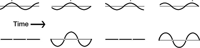
Waves may be either traveling, wherein a pulse propagates along a medium, varying its position in space over time, or standing, wherein important spatial features of waves, known as its nodes and antinodes, remain fixed in space (see fig. 1). A particularly well-known example of standing waves occurs in acoustics, where vibrating strings and air columns produce the heard tones of musical notes; standing waves also occur in lasers, river flows, seismic phenomena, and mechanical resonance.
Comparison between a traveling (top) and standing (bottom) wave. Gray dots indicate the progress of a single wave crest along the length of the line (top). White dots indicate stable nodes in the standing wave (bottom).

Different mathematical models are used for traveling waves than for standing waves. Traveling waves are modeled with wave equations in which vertical displacement is expressed as a function of time, horizontal position, amplitude, wavelength, and frequency. Standing waves, however, are modeled with wave equations in which vertical displacement is expressed as a function of time, horizontal position, amplitude, frequency, length of the vibrating body (I will consider a vibrating string below), and harmonic ordinal. The standing-wave equation is a solution to the traveling-wave equation.
The physics of these two classes of phenomena, and the mathematics of these two classes of models, are distinct but closely related. A common and intuitive explanation of the relationship between traveling and standing waves is that standing waves may be understood as the sum of two traveling waves of identical velocity and phase, moving in opposite directions along the same medium. These two component waves interfere with one another, and because the waves are identical save their direction, the interference is constructive: the amplitudes of the crests and troughs are doubled, rather than canceled out by one another, as they would be if the component waves were not in sync. In physical systems, many standing waves genuinely evolve in this manner from traveling waves that initiate motion in a localized position on the medium, although it is possible to directly transmit standing waves across media.
Two further points about standing waves are necessary for the current discussion. First, it is impossible to generate a standing wave in a medium with an indefinite or changing length and without at least one fixed end. Fixing the end of the medium forces the energy generated by the wave to be reflected back into the system once it encounters that unmoving boundary. If the endpoint were not fixed, that is, if it moved around, the wave would dissipate on impact with the boundary via destructive interference. Rather than the lossless reflection of energy through a fixed point that produced the standing wave, reflecting a wave through a moving boundary will demolish the standing wave through destructive interference and dissipative exchange with the environment. Further, conservation-of-momentum principles dictate that waves, whether traveling or standing, will flip their pulse (i.e., move from positive to negative vertical displacement or vice versa) upon contact with a fixed boundary.
Second, the harmonic ordinal n is a particularly important parameter in the modeling of standing waves. It can take positive integer values, and it specifies whether a particular standing wave has the lowest frequency supported by the medium, second lowest, or so on. A given vibrating medium can only support certain frequencies, and thus certain wavelengths, of a standing wave. For instance, a vibrating string of length L can only generate standing waves with wavelengths of 2L/n.Footnote 1 Especially in acoustics,  is known as the fundamental tone or first harmonic, and
 and higher are known as the medium's harmonics, referred to by ordinals (
 is the second harmonic,
 is the third harmonic, etc.). In music, harmonics are so central to theory and composition that they comprise their own chapters in many tutorial books. There is even a musical notation symbol for the playing of a note to emphasize a particular harmonic, a technique popularized in the 1700s that is common notation in contemporary compositions.
4.2. Three Explanatory Functions
These technicalities provide sufficient detail to see the following point: in modeling waves, to specify that the medium has a definite length and that the system has at least one fixed endpoint is to specify boundary conditions on the system. The traveling-wave equations of motion say nothing about what happens when a wave encounters the edge of the medium in which it is propagating; instead, as described above, conservation principles external to the wave equation dictate that when a wave reaches the end of the medium, if the end is fixed, the wave will be reflected back with a flipped pulse. If not, the wave will dissipate through the motion of the medium's edge in interaction with its environment, as well as through destructive interference with the portions of these dissipated waves that reflect along the length of the medium. Holding the endpoint fixed adds a component to the model of the system, and this addition enables the generation of new patterns, specifically the patterns modeled by the standing-wave solution to the wave equation.
Recognizing the specification of a fixed endpoint as a boundary condition in the model of a standing wave enables two philosophical observations. First, it provides another illustration of the distinction I drew above between the variable-fixing and structure-specifying modes of understanding the explanatory role of boundary conditions. In the variable-fixing mode, the question of whether a given system is fixed or mobile at its endpoint is merely a contingent fact about the system, but in the structure-specifying mode, fixing the endpoint generates a pattern of further conditions on models of the system's behavior accessible only through standing-wave modeling.
This latter function builds to the second observation, which is that boundary conditions enable the application of certain classes of model to a system. This furnishes the first explanatory function of boundary conditions:
Boundary Conditions Set the Scope of Models. Specifying boundary conditions can limit the scope of a model to a limited subclass of systems to which a set of governing equations applies. Examples include fixing an endpoint on a vibrating string in order to access standing-wave models and setting a no-slip condition on a fluid flow.
It is widely recognized that specifying scope is a precondition for building explanations, and most of the accounts of model-based explanations referenced above address scope-setting explicitly. For instance, in her account of how models explain, Bokulich has argued that model-based explanations in particular require a “justificatory step,”? in which an explainer “specif[ies] what the domain of applicability of the model is, and show[s] that the phenomenon in the real world to be explained falls within that domain”? (Reference Bokulich2008, 226). In cases like specifying slip and endpoint fixing, changing the boundary condition changes the scope, or domain of applicability, of the model. It also changes what model is being used within the scope, for example, from a traveling-wave model to a standing-wave model, which generates further restrictions on how an explanation is to be constructed. In Bokulich's terms, would-be explainers will have to perform different demonstrations to show that a phenomenon falls within the domain of a standing-wave model rather than a traveling-wave model.
I have given the scope-setting example in terms of fixing the endpoint on a wave medium, but the same point holds for setting a definite length on the medium. Modeling a wave as moving through a medium of a fixed length, as opposed to an indefinite or variable length, generates new information about the system by restricting the possibilities for what happens at the system's edge. This occurs in two ways: (1) modeling a traveling wave as moving along a medium of length L indicates where a given wave's vertical displacement (and velocity and acceleration) will be when it reaches the edge of the medium, provided the starting location of the wave is known, and (2) the existence of a definite L indicates that there will be certain wavelengths for which constructive interference is possible, as well as indicating that if the system were to evolve a standing wave, its first harmonic would be at wavelength 2L/n.
Specifying that the medium has definite length and fixed endpoints enables the application of the standing-wave model in the scope-setting manner identified above, but it also provides an illustration of the second, related explanatory function of boundary conditions. By generating rules about what happens at the edges of models, boundary conditions enable the stable application of governing equations to the interior behavior of a system.
Boundary Conditions Enable Stable Descriptions of Law-Like Behavior. Through specifying what occurs at the edge of a modeled system, boundary conditions enable the production of stable descriptions of the system's interior behaviors.
This is the explanatory function of boundary conditions that Wilson conjures in his discussion of modeling billiard balls (see sec. 3.2 above). Elsewhere in that discussion, he describes how “interior modeling equations nonetheless demand crude descriptions of these exterior regions; otherwise all the reasoning advantages offered by differential equations modeling will vanish”? (2017, 36). These “reasoning advantages”? are an instance of the titular phenomenon in the book from which the passage was drawn: Wilson's Physics Avoidance (Reference Wilson2017). “Physics avoidance”? is Wilson's characterization of the combination of idealizations, abstractions, and tools of mathematical reasoning (e.g., variable reductions, renormalizations) that comprise the strategy of systematically ignoring certain details of physical systems in order to obtain stable descriptions of patterns of behavior. Imposing boundary conditions on models of physical systems enacts this physics-avoidance strategy in a notable way, namely, by parameterizing away certain particularities and details of the complex behaviors that occur at the edges of physical systems. This parameterization is necessary for producing models capable of describing patterns of behavior at all: if every detail of a physical phenomenon were required to be represented in a model, the familiar and lamentable chaos of oversubscription to detail would ensue.Footnote 2
Returning to the wave example, fixing the endpoints of the wave medium is what gives rise to the conceptual possibility of any standing wave whatsoever, as well as to the possibility of a flipped wave pulse. If the endpoints of the medium move around, then there is no opportunity for the reflection of a wave: as discussed above, the wave will dissipate due to energy loss through an open boundary. It is impossible to access the system's harmonics, and any explanations they generate, without including fixed endpoints as a component of the wave model. To put the point another way, without fixed boundaries on the motion of a wave, there is no possibility for a standing wave to be generated. The wave equation only dictates how a wave will propagate. Because the very concept of a standing wave entails a notion of reflection through a fixed boundary, standing waves are strictly features of a system with fixed endpoints. Without fixed endpoints, the notion of a standing wave ceases to make sense, like a circle without a circumference, a mountain without a valley, or death without life.
This explanatory function of boundary conditions has been gestured at before, notably in Cartwright's (Reference Cartwright1999) account of “nomological machines.”? Cartwright's machines are systems consisting of a “fixed (enough) arrangement of components, or factors, with stable (enough) capacities that in the right sort of stable (enough) environment will, with repeated operation, give rise to the kind of regular behaviour that we represent in our scientific laws”? (50). In her view, these systems give rise to the conditions that permit scientists to observe law-like behavior and apply nomological reasoning to draw inferences and generate theories. Consequently, in her account, Cartwright's nomological machines perform the same sort of sanctioning as I am suggesting that boundary conditions do: like nomological machines, boundary conditions on models in physics specify regions where the laws will apply (function 1) and enable laws to produce stable descriptions of interior behavior (function 2).
Both the scope-setting and law-stabilizing functions of boundary conditions serve as logical preconditions on the construction of model-based explanations that appeal to the equations of motion in mathematical models, no matter whether one interprets those equations as laws, governing equations, or mathematical or causal regularities. The third function of boundary conditions concerns their ability to generate new phenomena that can serve as explanantia in such explanations.
Boundary Conditions Generate Phenomena. Placing boundary conditions on a model of a physical system can produce novel phenomena that cannot be predicted from or explained by equations of motion alone.
In the fluid-mechanical case discussed earlier, specifying whether slip occurred in a modeled system enabled the application of Navier-Stokes models to explanations of a system's behavior. In cases in which slip occurs, specifying slip did not necessarily end an explanatory or modeling investigation. Instead, slip itself became a target for the construction of models and explanations. This is the origin of Prandtl's boundary-layer models in fluid mechanics, which Morrison has argued are an importantly phenomenological set of mathematical models in physics (Morrison Reference Morrison, Morgan and Morrison1999, 53”?54). By this she does not mean to draw a contrast with theory but rather to emphasize that the Prandtl models were constructed specifically to generate the ability to represent, examine, and explain the particular phenomenon of the flow of a thin boundary layer at the edge of a bulk fluid flow. Prandtl initiated development of the boundary-layer model in response to the mathematical intractability of the Navier-Stokes equations in instances when the boundary condition specified partial slip.
Analogously, in wave physics, the stable nodes and relations among harmonics in standing waves are phenomena that are inaccessible from the equations of motion of either traveling or standing waves alone. They appear only through the specification of the boundary conditions on a standing wave (determinate length and fixed endpoints), and the harmonic relation in particular has become a subject of mathematical and physical investigation in its own right. It has given rise to an entire branch of mathematics, namely, harmonic analysis, which includes the techniques of Fourier analysis and can be applied to problems in optics, condensed matter, and quantum mechanics, as well as synaptic behavior and tidal modeling.
I call attention to these theoretical investigations on boundary phenomena not for their own sake but to emphasize that such phenomena exist and have been initially noticed through the specification of boundary conditions. Further, it is not uncommon for explanations of the sort that appeal to the mathematical models in which conditions are a component to appeal, also, to such phenomena. For instance, explanations of the mathematical relations among harmonics typically appeal to the location of nodes along the length of the medium, using geometric reasoning to rationalize why nodes appear in certain locations on the medium and not others. Setting the acoustic boundary conditions generates new phenomena that can be used in the construction of explanations in acoustics. In this way, boundary conditions broaden and change the available explanatory landscape.
4.3. A Final Function: Coordinating Models
The final explanatory function of boundary conditions is somewhat distinct from the first three, because it considers the role of boundary conditions not only within a particular model but as a means of generating conceptual, mathematical, and explanatory bridges between models in multimodel explanations:
Boundary Conditions Coordinate Multimodel Explanations. Through the parameterization of messy edge phenomena, boundary conditions are able to facilitate the exchange of information among different mathematical models from different theoretical backgrounds in the construction of explanations that draw on multiple modeling frameworks.
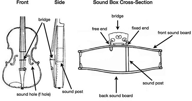
This function of boundary conditions is best explicated through a more extended example. In wave physics, an important class of explanations of acoustic phenomena arises from questions like, “Why does a violin sound like a violin?”? In order to answer this question, acoustic physicists employ not only models of the sound waves produced by the instrument(s) in question but also models of the methods of production of those sound waves, that is, of the structure of the violin. In violins, audible tones are produced when the violinist generates a resonant vibration in one or more of the instrument's strings. Vibrations in the string produce vibrations in the bridge, which is the thin piece of wood that raises the four strings away from the body of the instrument. Vibrations in the bridge are then transmitted to the instrument's body through the bass bar and the sound post (see fig. 2). This induces vibrations in the sound box, that is, the hollow in the wooden body of the instrument, which amplifies the sound and transmits it into the air. Most acoustical study of sound production in violins centers around questions of the relationship between the instrument's components, the materials from which they are made, and the wave energy loss associated with each stage in the transmission process described here.
Anatomy of a violin's sound box. Adapted from Creative Commons licensed sources.

When a violinist draws her bow along a properly tuned open A string, her bow induces a vibration in the string. In the first instants of the string's excitation, the bow produces traveling waves at a variety of frequencies, which propagate down the length of the string. However, as per the strictures of wave physics discussed above, only certain frequencies will persist through reflection at the fixed endpoint of the string, and only these frequencies participate in the resultant, resonant vibration, which is recognizable as a standing wave in the string. That standing wave occurs at a fundamental frequency of 440.0 Hz, creating a sound wave with a wavelength of approximately 78 cm.
The singular texture and shape of a note played on a violin arises from the specific combination of fundamental and harmonic tones produced by the particular bowing or plucking of that particular string and transmitted through the materially contingent resonance chambers in the violin's body. This is what makes a note on a violin sound like a violin, and it is what makes that violin sound like that violin. Every violin is unique, and instrument makers and acousticians alike study the material properties of woods, varnishes, animal and metal strings, bow designs, rosin types, and other material constituents of the instrument, as well as the acoustic impacts of differences in ambient temperature, humidity, and air pressure. Nonetheless, violins tend to sound like violins, and the notes they produce generate different sounds than notes in the same register produced by other instruments: a violin does not sound like a piano, or a flute, or a tuning fork.
There is an apparent incompatibility between the model of the violin's sound transmission and the model of the string's harmonics. Holding the endpoints of the vibrating string fixed is necessary to generate a standing wave, as discussed extensively above. However, holding the endpoints of a violin string fixed is also antithetical to deriving explanations from the transmission model: if the end of the violin string that touches the bridge is fixed and still, the violin is silent—without a moving bridge, there is no vibration to communicate to the sound post, sound board, instrument body, or the air beyond. The two models contributing to an explanation of violin acoustics are, it appears, incompatible, despite that both are fundamentally about the production of sound waves.
Resolving this apparent incompatibility is a crucial step in developing a theory of explanation. Similar problems have been encountered elsewhere in explanation in physics, and philosophers of science have developed a variety of coping mechanisms: one model of the system might be reduced to the other, or one might turn out to emerge from the other as a limiting case, so that the two models on which the explanations are based are no longer competing over the same explanandum. The problem with this approach is that reductive and emergent strategies for linking models or theories together typically rely on some kind of separation along the length, time, or energy scales involved in the component models, so that it is possible to cleave one model off from another. In modeling a violin's acoustics, however, there is no meaningful distinction between the length, time, and energy scales involved in the waves described by the harmonics model and those described in the structural model of the violin's sound box. The problem is not one that can be easily resolved by separation of levels or scales. In a similar vein, there is no obvious ordering of the two models along the dimension of fundamentality. The harmonics explanation is not about a more fundamental piece of the sound production than the vibration-transmission explanation or vice versa. But if the two explanations are about the same thing, and if they are both essential to understanding violin acoustics, then there should be some way to reconcile the two—especially since the models that generate these explanations are in fact often pooled together in physical explanations of violin acoustics.
The resolution, I believe, lies in the role of the fixed endpoint as a boundary condition on the model of the string's harmonics. In performing the second and third explanatory functions identified above, the fixed endpoint of the harmonic model is essential in generating explanations of the violin's harmonics. However, it is a point of fact that the boundary at the bridge end of the violin simply is not genuinely fixed: it wiggles around and is designed specifically to do so, and it does so in a way that transmits vibrations from the bridge through the various parts of the violin and out into the world. What fixing the endpoint in the harmonic model does is to idealize away the wiggling, so that it is possible to produce a model of the string's behavior that successfully generates the harmonic relations of interest. Holding the endpoint fixed in the model is an example of Wilson's physics avoidance, in which the complicated dynamics of the actual points of contact between the string and the bridge are suppressed in order to enable the production of patterns of behavior in the model. Once those patterns of behavior (i.e., the harmonics) are obtained from the harmonic model, it is possible to export them into the model of sound transmission.
A small aside may prove useful. How information can be transmitted across multiple models in a multimodel explanation is a subject of significant recent philosophical interest, particularly as it pertains to the construction of multiscale models (e.g., as in Winsberg Reference Winsberg2010; Green and Batterman Reference Green and Batterman2017; Bursten Reference Bursten2018; Jhun Reference Jhun2019). In a recent article on multiscale modeling, for instance, I argued that the use of a multiscale model is only justified to the extent that the “conceptual strategies”? connecting the component models in the multiscale model are justified (Bursten Reference Bursten2018). These strategies draw on a combination of mathematical, theoretical, and empirical background information to rationalize a particular way of stitching multiple component models together. The model-connecting function of boundary conditions illustrated here may be understood as a type of such a conceptual strategy. Acknowledging that setting the boundary condition in the harmonic model is an instance of physics avoidance provides justification for exporting harmonic phenomena into the transmission model. This is itself an instance of Bokulich's justificatory step in constructing model explanations. Treating the contact between the violin's string and bridge as a fixed endpoint, and thus modeling it as a reduced-dimension boundary condition, are elements in the construction of a conceptual bridge between the harmonics and transmission models.
The specification of a boundary, and the encoding of that boundary into a boundary condition on a mathematical model, are nearly universal preconditions for the generation of explanations in the physical sciences. Further, there are plenty of domains of physics that require careful study of how certain features of a system are represented sometimes as boundary conditions and sometimes as robust physical behaviors with internal mechanics of their own. The technique of idealizing away complex behavior at material boundaries by parameterizing that behavior is a crucial step in building successful multiscale models and resolving the problem of the tyranny of scales, as discussed by Batterman, Phillips, and others (Phillips Reference Phillips2001; Oden et al. Reference Oden, Belytschko, Fish, Hughes, Johnson, Keyes, Laub, Petzold, Srolovitz and Yip2006; Batterman Reference Batterman and Batterman2012). Indeed, it may be the case that most, if not all, explanations in physics that employ multiscale models rely essentially on the use of boundary conditions to coordinate among theoretical backgrounds. Even mechanistic explanations, in which impulses are transmitted from one part of a system to another, need a story about how the force from one billiard ball produces motion in a second ball, and the microphysics of such interactions must be reconciled with the macroscopic notion of a perfectly elastic collision.
To return to the account being developed here, the final explanatory function of boundary conditions is to coordinate different models, often with distinct theoretical backgrounds, into a single explanation. I have illustrated this connective function through the example of violin acoustics, but a similar story could be told about the production of explanations that employ both Navier-Stokes and boundary-layer flow models in fluid mechanics and across a variety of other contexts, as well. This function is distinct from the first three in that it occurs only in the construction of explanations that employ multiple models, rather than being applicable to either single-model or multiple-model explanations.
5. Conclusion
The four explanatory functions of boundary conditions share a few common features: they articulate distinctive roles for boundary conditions in the project of constructing physical explanations from models, and those roles are derived from what I have called the structure-specifying way of understanding boundary conditions, rather than the variable-fixing way of understanding them. In explicating these explanatory roles I have occasionally explicitly distinguished between attributing an explanatory fact or feature to a boundary condition as opposed to a law. However, in other places—for instance, in the explanation of the transmission model of a violin's sound production—laws have been left largely out of the developing picture. The four functions are meant to exist in a compatibilist pluralism with one another: as seen in the examples given, some individual roles for boundary conditions occupy multiple functions, and not every function is instantiated in each application of a boundary condition to the development of an explanation.
My motivating aim in articulating this account has been to argue against the two Hempelian theses about the role of boundary conditions in physical explanations, largely because these theses have been persistent in the philosophy of science and pernicious to our understanding of explanation. The picture I have painted is one of boundary conditions as components of models that can set the scope of law-like claims, rationalize the existence of stable behavior in the interior of modeled physical systems, generate phenomena with explanatory value, and coordinate between models with differing theoretical backgrounds. This picture is intended as substantial evidence against the Hempelian thesis 2, namely, that laws always play the more central role in physical explanation.
Part of this evidence comes from the substantial, irreducible, and varied functions of boundary conditions in the sorts of explanations I consider here, but another bulk of the evidence comes from the argument contained in section 3, which offered reasons to reject the conception of boundary conditions as the non-law-like components of explanations. I closed that section with a discussion point that is important enough that it merits restating here: the role of contingent facts in scientific explanation is an important subject to be able to reference in philosophical discussions of explanation, but it is a mistake to refer to that subject by talking about the boundary conditions, or initial and boundary conditions, of a system. Doing so invokes the variable-fixing, rather than the structure-specifying, conception of boundary conditions, which is the wrong one to attend in considering the function of boundary conditions in physical models. It also has the consequence of steering attention away from the varied and complex functions of boundary conditions in physical explanation. To paraphrase Butterfield: variable fixing is a matter of mere happenstance, in some sense that structure specifying is not.
There is a more limited sense in which some contingent properties of materials may be represented by or interpreted as initial conditions in some physical models, insofar as initial conditions specify the state of affairs at the outset of the evolution of a dynamical system. This constitutes evidence against thesis 1, since initial conditions can be understood as occupying some of the same conceptual territory as contingent facts. However, just as boundary conditions are well-defined mathematical objects, so are initial conditions; likewise, just as boundary-value problems carve out a host of interesting challenges for physical modeling and its epistemology, so may initial-value problems. I have not conducted a study on initial conditions to parallel the present considerations on boundary conditions, but it seems evident that initial conditions will not function to rationalize stable behavior, generate phenomena, or coordinate models in the same manner as boundary conditions. That said, they may, in some sense, limit scope in a parallel fashion.
However, important distinctions remain between initial conditions and boundary conditions. Unlike initial conditions, boundary conditions place enduring constraints on the behavior of wave and fluid systems, fixing the spatial regions where the laws will apply. It is not just the wave equation, but instead the paired team of the wave equation coupled with fixed endpoints, that drives explanations of harmonics. The notion of reflection through a boundary point is crucial to the generation of a standing wave; remove it, and the only options left to the wave are propagation and dissipation, neither of which will produce a violin's note. In modeling the evolution of a standing wave, the initial condition specifies the amplitude and the location of the initial traveling wave, which resolves into the standing wave once it reflects through the fixed boundary points. True enough, differences in initial conditions can affect the amplitude and harmonic ordinal of the resulting wave, but differences in initial conditions do not constrain the possible frequencies of the standing wave. To put the point in terms of the violin example, an open A string will always play A as its fundamental tone, no matter whether it is bowed heavily or lightly, next to the bridge or up on the neck of the instrument. The boundary endures, and with it, the boundary conditions on the mathematical model. This indicates that there is a meaningful difference between the explanatory roles of initial conditions, on the one hand, and of boundary conditions, on the other.
Taken together, these observations are intended as a corrective to the canonical philosophical use of the term “boundary condition”? in discussions of scientific explanation. Boundary conditions are mathematical objects that are components of models in physics. They serve at least four distinct explanatory functions: scope setting, law stabilizing, phenomena generating, and model coordinating. These functions are not mutually exclusive, and more work remains to be done in articulating how the different functions relate to one another. Nonetheless, the functions can be slotted into a variety of contemporary accounts of explanation, and they are particularly apt for use in accounts of model-based explanation, where they can be interpreted as supporting the generation of explanatory patterns in models. Finally, to mistake boundary conditions for contingent facts is, at best, a bad joke.