


1. Introduction
For a long time, the occurrence of near-wall reverse flow (NWRF) in a zero-pressure gradient (ZPG) turbulent boundary layer (TBL) seemed impossible. This view was influenced by the work of Eckelmann (Reference Eckelmann1974), who studied the flow structure in the viscous sublayer, concluding that ‘it can be stated with certainty, therefore, that there are no negative velocities near the wall’. The experimental study of Colella & Keith (Reference Colella and Keith2003), performed relatively recently, indirectly confirmed this statement showing that ‘the probability density of wall shear stress fluctuations … exhibits no flow reversals at the wall’. However, Spalart & Coleman (Reference Spalart and Coleman1997), Hu, Morfey & Sandham (Reference Hu, Morfey and Sandham2006), Lenaers et al. (Reference Lenaers, Li, Brethouwer, Schlatter and Örlü2012), Cardesa et al. (Reference Cardesa, Monty, Soria and Chong2014, Reference Cardesa, Monty, Soria and Chong2019), Brücker (Reference Brücker2015), Vinuesa, Örlü & Schlatter (Reference Vinuesa, Örlü and Schlatter2017), Diaz-Daniel, Laizet & Vassilicos (Reference Diaz-Daniel, Laizet and Vassilicos2017), Willert et al. (Reference Willert2018), Jalalabadi & Sung (Reference Jalalabadi and Sung2018), Bross, Fuchs & Kähler (Reference Bross, Fuchs and Kähler2019) and Chin et al. (Reference Chin, Vinuesa, Örlü, Cardesa, Noorani, Chong and Schlatter2020) demonstrated the existence of NWRFs numerically and experimentally, so that today their existence is widely accepted. However, the mechanism of their occurrence in ZPG TBLs is still under debate.
Spalart & Coleman (Reference Spalart and Coleman1997) were the first to draw attention to this flow feature. They found negative values of the streamwise component of the wall shear stress using direct numerical simulations (DNS) of ZPG TBLs. Furthermore, the presence of NWRFs was numerically shown by Hu et al. (Reference Hu, Morfey and Sandham2006), who observed an increase in the probability,  $P$, of negative values of the streamwise component of the wall shear stress with an increase in the friction Reynolds number,
 $Re_\tau$, from
 $P=0.003\,\%$ for
 $Re_\tau =90$ up to
 $P=0.0854\,\%$ for
 $Re_\tau =1440$. At this time, NWRFs were considered in a statistical sense, and no attempt was made to explain the underpinning mechanisms or to characterise these flow features in detail. Lenaers et al. (Reference Lenaers, Li, Brethouwer, Schlatter and Örlü2012) studied the generation mechanism of NWRFs, concluding that they are caused by extremely strong oblique vortices existing in the buffer region. They were typically observed underneath large-scale high- and low-momentum (H-M and L-M, respectively) coherent flow structures existing in the log-law region, with L-M-related events detected less frequently. Their observations contradict the recent high-resolution two- and three-dimensional particle image velocimetry (PIV) studies by Bross et al. (Reference Bross, Fuchs and Kähler2019), who considered adverse pressure gradient (APG) TBLs at
 $Re_\tau =5000$ and Clauser pressure gradient parameter
 $\beta = 13.5 - 14$. They concluded that a necessary condition for NWRFs is the superposition of large-scale L-M flow structures with low-speed near-wall streaks representing a part of vortices existing in the buffer region. Furthermore, they showed that a strong near-wall vortex should either have a spanwise orientation or be slightly tilted in a streamwise direction. This complex interaction of streaks with L-M structures justifies the rare occurrence of NWRFs, while the possible orientation of a near-wall vortex explains two characteristic forms of NWRFs. Thus, both Lenaers et al. (Reference Lenaers, Li, Brethouwer, Schlatter and Örlü2012) and Bross et al. (Reference Bross, Fuchs and Kähler2019) associate NWRFs with these vortical structures in the buffer region, while observing different correlations with large-scale flow structures existing in the log-law region.
Vinuesa et al. (Reference Vinuesa, Örlü and Schlatter2017) observed different mechanisms of NWRF formation for low ( $\beta \approx 0.6$) and high (
 $\beta > 4.1$) APGs. Considering the flow around the NACA4412 wing, they confirmed the existence of the mechanism associated with the near-wall oblique vortex structures at low and moderate values of APG (
 $\beta < 4.1$). On the other hand, their visualisations did not reveal the correlation of NWRFs with near-wall coherent structures for higher APGs (
 $\beta > 4.1$), contrary to observations of Bross et al. (Reference Bross, Fuchs and Kähler2019). Therefore, they suggested that the NWRF phenomenon may be associated with the outer region of a TBL with an increase in the pressure gradient, rather than near the wall. Vinuesa et al. (Reference Vinuesa, Örlü and Schlatter2017) showed that NWRFs become more frequent with the increase in APG, reaching a probability of their occurrence of 30 % for considerable pressure gradients. This is a manifestation of a separating flow where NWRFs exhibit a smaller transverse component. For moderate values of
 $\beta$, Vinuesa et al. (Reference Vinuesa, Örlü and Schlatter2017) obtained NWRFs with a very high probability of about 10 % for
 $Re_\tau \simeq 336$,
 $\beta \simeq 12$ compared with
 $P=1.7\,\%$ presented by Bross et al. (Reference Bross, Fuchs and Kähler2019) for
 $Re_\tau = 5000$,
 $\beta \simeq 14$. This does not fit the general trend that the NWRF probability increases with the Reynolds number (Hu et al. Reference Hu, Morfey and Sandham2006; Lenaers et al. Reference Lenaers, Li, Brethouwer, Schlatter and Örlü2012). However, the history effects should also be considered when comparing APG flows as different incoming flow histories can lead to significant changes in the Reynolds stress distribution and the statistical properties of the flow (Bobke et al. Reference Bobke, Vinuesa, Örlü and Schlatter2017). It is worth noting that the outcome of a statistical data processing procedure applied to NWRFs may be sensitive to their generation mechanism depending on the flow configuration shaping the specific topological features. The spatial extensions of NWRFs may also depend on the flow type as with the presence of the pressure gradient (Vinuesa et al. Reference Vinuesa, Örlü and Schlatter2017; Bross et al. Reference Bross, Fuchs and Kähler2019).
Almost simultaneously with Lenaers et al. (Reference Lenaers, Li, Brethouwer, Schlatter and Örlü2012), Chong et al. (Reference Chong, Monty, Chin and Marusic2012) showed that the cause of NWRF onset is the presence of three-dimensional structures near the wall. They came to this conclusion studying critical points of the skin friction and vorticity, which are closely related to NWRF. Using the results of direct numerical simulations (DNS) of Alamo et al. (Reference Alamo, Jiménez, Zandonade and Moser2004), they showed that the NWRF region is always accompanied by a pair of saddle-node critical points, indicating the existence of a complex three-dimensional separated flow near the wall, leading to negative values of the skin friction. In fact, their study is a continuation of their earlier work (Perry & Chong Reference Perry and Chong1986), where the possible existence of the NWRF events was theoretically predicted for the first time. Experimentally, the existence of critical points of the skin friction was confirmed by Brücker (Reference Brücker2015) when studying ZPG TBLs at  $Re_\tau =940$ by visualising the flow in the near-wall region for
 $y^{+}<10$, where the ‘
 $+$’ superscript denotes wall units. They observed a vortex structure inclined in a wall-parallel plane, indicating that the negative streamwise wall shear stress also stemmed from regions where the transverse component was of considerable magnitude. This is fully consistent with the results of Lenaers et al. (Reference Lenaers, Li, Brethouwer, Schlatter and Örlü2012), Diaz-Daniel et al. (Reference Diaz-Daniel, Laizet and Vassilicos2017) and Bross et al. (Reference Bross, Fuchs and Kähler2019). Another set of experiments was performed by Willert et al. (Reference Willert2018) confirming the NWRF existence employing PIV measurements in the near-wall region of ZPG air flow at
 $Re_\tau =1000$ and
 $2700$.
The flow field around critical points was extensively studied by Cardesa et al. (Reference Cardesa, Monty, Soria and Chong2014, Reference Cardesa, Monty, Soria and Chong2019) who observed them at the tail of large-scale flow structures that extended from the wall to the outer edge of the log-law region of a TBL at a distance of  $x^{+} = 800$ downstream of critical points. At the same time, they showed the existence of a strong spanwise vortex directly above the critical point, which was created by the action of the vortex being pushed sufficiently close to the wall. The spanwise vortices observed by Cardesa et al. (Reference Cardesa, Monty, Soria and Chong2014, Reference Cardesa, Monty, Soria and Chong2019) at the tail of the large-scale L-M flow structures can be explained by the interaction of oblique quasi-streamwise or transversely oriented vortices with the most decelerated region of the large-scale L-M flow structures. Such vortices were observed by Lenaers et al. (Reference Lenaers, Li, Brethouwer, Schlatter and Örlü2012), Brücker (Reference Brücker2015), Vinuesa et al. (Reference Vinuesa, Örlü and Schlatter2017), and Bross et al. (Reference Bross, Fuchs and Kähler2019) as well. The flow pattern described is similar to the one observed by Bross et al. (Reference Bross, Fuchs and Kähler2019) for APG TBL, but with two conceptual differences. Firstly, NWRF events observed in ZPG or low-pressure gradient TBLs appear at the tail of the L-M flow structures rather than in its entire area, as is the case for high APG flows. Apparently, the flow in an APG TBL is already sufficiently slow to ensure the NWRFs occurrence over the entire length of the large-scale L-M flow structure. Secondly, we would like to clarify that the NWRF event is caused by some near-wall vortex rather than low-speed streak because the latter is simply an upward motion side of quasi-streamwise or transverse vortices.
A brief review confirms that it is generally accepted that NWRFs are associated with some strong near-wall vortical structures located in the buffer region; however, there is a difference in their correlation with large-scale flow structures existing in the log-law region. The present study aims to provide an insight into the mechanism of the NWRF formation including the role of the far-field flow region.
2. Numerical and experimental details
We describe the numerical and experimental methods employed to study NWRFs in a duct flow of a square cross-section with  $H$ serving as the half-width of the duct. We consider a relatively low Reynolds number
 $Re=U_bH/\nu =3150$ for DNS and
 $Re=3100$ for PIV, with
 $U_b$ and
 $\nu$ representing the bulk velocity and kinematic viscosity. While at these Reynolds numbers the spatial resolution is not an issue, NWRFs become very low-frequency events, as discussed in this paper's introduction, requiring large computational time intervals for DNS as well as time-consuming measurement routines. Owing to the finite dimensions of the sensing element of the camera used in PIV with the given optical system, the measurement area is small enough to enable the study the outer layer. However, it is sufficient to accurately validate DNS results with the low probability of the NWRF occurrence (see figure 4(a) for details). To our knowledge, there are no experimental data on the NWRF phenomenon for
 $Re_\tau < 1000$, except for the work of Brücker (Reference Brücker2015) where only the probability of the NWRF occurrence at
 $Re_\tau =940$ is provided. Note that the mechanism may differ for flows with low and high Reynolds numbers owing to different scales of flow structures in the log-law region, i.e. large-scale structures for low Reynolds number and so-called superstructures for high Reynolds number.
2.1. DNS
We used the computational code Nek5000 featuring a semi-implicit third-order time integration scheme and spatial discretisation based on the spectral-element method (Fischer et al. Reference Fischer, Kruse, Mullen, Tufo, Lottes and Kerkemeier2008). The Navier–Stokes equations were discretised in space with the use of the Galerkin approximation and 8th-order Lagrange polynomial interpolants based on the Gauss–Lobatto–Legendre points for both the velocity and pressure fields ( $P_N-P_N$ formulation). We considered a computational domain of size
 $L_x \times L_y \times L_z = 2 {\rm \pi}H \times 2H \times 2H$ in the streamwise, wall-normal, and spanwise directions, respectively, with
 $18 \times 32 \times 32$ spectral elements corresponding to
 $N_{tot}=9.4 \times 10^{6}$ mesh points. A no-slip boundary condition was imposed at all walls, while the periodic condition was applied in the streamwise direction. After reaching a steady-state turbulent flow regime, we collected data within a time period of
 $TU_b/H = 250$ corresponding to
 $T^{+}=Tu^{2}_\tau /\nu =3308$ in wall units, where
 $u_\tau$ is the perimeter-averaged friction velocity and
 $\nu$ is the kinematic viscosity with the friction Reynolds number of
 $Re_\tau = u_\tau H/\nu = 204$ for this case. For further comparison with experiments it is convenient to introduce the friction velocity
 $u_{\tau ,c}$ in the symmetry plane (centreplane) leading to the corresponding Reynolds number
 $Re_{\tau ,c} = 211$. The comparison of the computational parameters in the present DNS with other simulations is shown in table 1.
Simulation parameters compared with the data from the literature.

The wall regions with negative values of the streamwise component of the wall shear stress  $\tau _x<0$ were associated with NWRFs. We interpolated numerical results on a regular mesh with a DNS-like resolution for post-processing. We used a mask of eight neighbouring mesh cells lying on the wall to identify NWRF regions as in Cardesa et al. (Reference Cardesa, Monty, Soria and Chong2019) who used a three-dimensional array of 27 mesh cells to identify the NWRF. A separate NWRF region consisted of connected mesh cells sharing the
 $\tau _x<0$ condition and was surrounded by a region with
 $\tau _x>0$. The coordinates of each NWRF region were determined as the coordinates of the centre of mass of a
 $\tau _x$ distribution. When performing the conditional averaging, all the NWRF regions were centred around the point
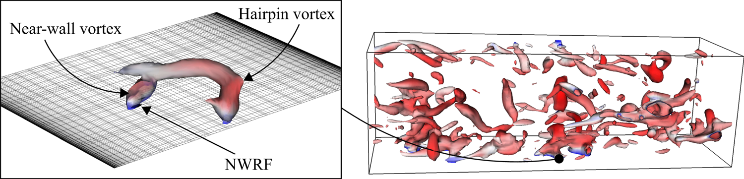
 $(0, 0, 0)$. The NWRFs appearing only at a single time step, as well as the ones crossing the boundaries of the computational domain, were not taken into account, providing in total a set of 158 independent NWRF events. The overall condition of the flow field is demonstrated in figure 1. The iso-surface of pressure demonstrates the population of coherent structures occupying the NWRF region.
Visualisation of the flow structures using instantaneous iso-surface of pressure coloured by streamwise velocity magnitude. Flow is from left to right. The NWRF region is marked by the arrow.

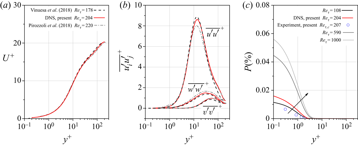
We compared our DNS results with those obtained by Vinuesa et al. (Reference Vinuesa, Schlatter and Nagib2018) and Pirozzoli et al. (Reference Pirozzoli, Modesti, Orlandi and Grasso2018) in similar computations with respect to  $Re_\tau$, see table 1. Figures 2(a) and 2(b) illustrate excellent agreement for the time-averaged streamwise velocity component as well as correlations of velocity fluctuations. Our results accurately fit between the other two DNS profiles reflecting the trend of
 $Re_\tau$ increase. Figure 2(c) shows the distribution of the NWRF probability against the wall distance from the present duct computation compared with turbulent channel flow in the range
 $Re_\tau =180 - 1000$. Our DNS results follow the general trend of the increase of
 $P$ with
 $Re_\tau$ where the maximum appears close to the wall with the underestimation of
 $P$ in experiments, discussed subsequently.
Wall-normal profiles of (a) the mean streamwise velocity and (b) the correlations of velocity fluctuations in the centreplane of the duct obtained in the present DNS compared with data from Vinuesa et al. (Reference Vinuesa, Schlatter and Nagib2018) and Pirozzoli et al. (Reference Pirozzoli, Modesti, Orlandi and Grasso2018). (c) The NWRF probability for a range  $Re_\tau =180 - 1000$ using channel-flow data from Lenaers et al. (Reference Lenaers, Li, Brethouwer, Schlatter and Örlü2012). The arrow indicates the increase in the Reynolds number.

2.2. Experiments
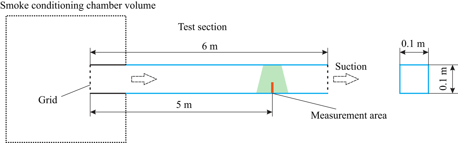
The PIV measurements were performed in a 6 m glass channel with a square cross-section of  $2H \times 2H = 0.1 \times 0.1\ \textrm {m}^{2}$, see the schematic diagram presented in figure 3. A constant air flow rate in the duct was maintained by a set of critical flow nozzles mounted between the compressor and the test section of the channel. A critical pressure drop for the nozzles at the considered flow rate was generated by a compressor. The relative error of the flow rate value did not exceed
 $0.25\,\%$. To organise uniform smoke seeding, the test section inlet was mounted in a smoke conditioning chamber of size
 $1.1 \times 1.4 \times 0.65\ \textrm {m}^{3}$. Prior to the experiments, the conditioning chamber was filled with smoke generated by Safex F2010 Plus and consisting of glycerine particles with a diameter of approximately
 $1\ \mathrm {\mu }\textrm {m}$. The uniformity of the incoming flow velocity profile and proper turbulent flow parameters were provided by a turbulence grid represented by a set of metal rods of diameter 1.3 mm and a grid spacing of 10 mm, mounted at the test section inlet. At a distance of approximately 2.5 m downstream of the entrance these manipulations led to a developing turbulent duct flow with an air temperature of
 $22\,^{\circ }\textrm {C}$. The bulk velocity in the duct was
 $U_b = 0.93\ \textrm {m}\ \textrm {s}^{-1}$ corresponding to a Reynolds number
 $Re = 3100$, which was close to the DNS parameters described previously. A set of measurements was made in the vertical symmetry plane of the duct at a distance of 5 m from the entrance where the turbulent flow was fully developed. The perimeter-averaged friction velocity could not be measured; however, the centreplane value
 $Re_{\tau ,c} = 207$ was close to
 $Re_{\tau ,c}=211$ obtained in DNS, see table 1. Note that a centreplane friction velocity,
 $u_{\tau , c}$, is also used when comparing experimental and DNS results.
Schematic diagram of the experimental facility.

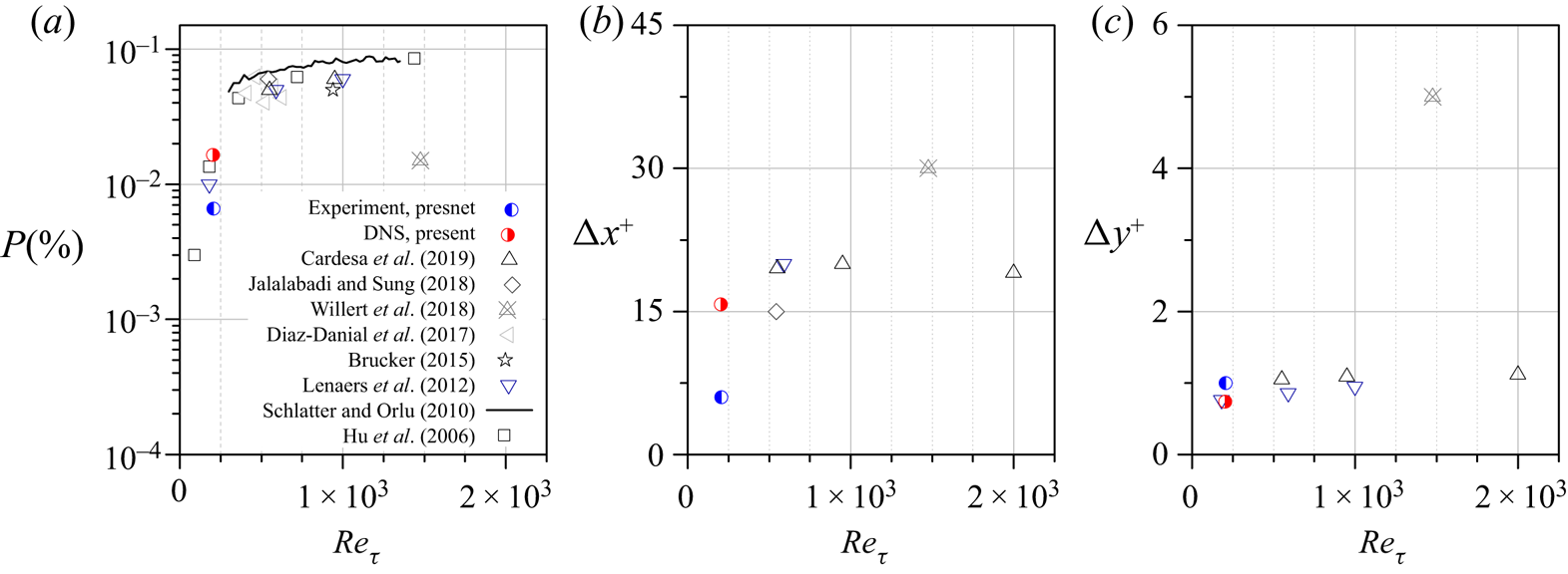
The NWRF regions are characterised by very small spatial extensions and low values of velocity of the order of the measurement error in many cases. Lenaers et al. (Reference Lenaers, Li, Brethouwer, Schlatter and Örlü2012) showed that the NWRF regions have an averaged shape of an ellipsoid flattened in the wall-normal direction with axes of  $\Delta x^{+} = 20$ and
 $\Delta z^{+} = 20$ aligned along the streamwise and spanwise directions and with an axis in a wall-normal direction
 $\Delta y^{+}$ slightly varying from
 $0.76$ to
 $0.95$ in the range of the Reynolds number
 $550 \leqslant Re_\tau \leqslant 2000$ (see figures 4b and 4c). Their data are in good agreement with those obtained by Cardesa et al. (Reference Cardesa, Monty, Soria and Chong2019). Jalalabadi & Sung (Reference Jalalabadi and Sung2018) showed slightly smaller spatial extension
 $\Delta x^{+}$ for their pipe flow compared with the one for channel flow (Lenaers et al. Reference Lenaers, Li, Brethouwer, Schlatter and Örlü2012; Cardesa et al. Reference Cardesa, Monty, Soria and Chong2019). The spatial extensions obtained experimentally by Willert et al. (Reference Willert2018) are much higher compared to other data. However, it should be noted that their data were obtained by visual inspection of the NWRF regions and therefore did not take into account their change in space and time, which should affect the mean values. Their NWRF probability is significantly underestimated, falling out of the general trend. Insufficient spatiotemporal resolution may be one of the reasons that experimental studies detect NWRF probability with several times lower values compared to numerical simulations. For instance, Lenaers et al. (Reference Lenaers, Li, Brethouwer, Schlatter and Örlü2012), relying on DNS data, showed that the spatial filtering procedure resulted in a significant underestimation of the results. The size of sensing elements in wall units used by Willert et al. (Reference Willert2018) varied from 12 to 20 in the streamwise direction and from 1.2 to 2 in the wall-normal direction. According to Lenaers et al. (Reference Lenaers, Li, Brethouwer, Schlatter and Örlü2012), these sizes are rather large to correctly detect such small structures as NWRFs. Moreover, weak NWRFs are usually discarded in experiments, possibly representing the measurement uncertainty.
(a) The NWRF probability and spatial extension of the NWRF regions in (b) the streamwise and (c) wall-normal directions. This figure represents a generalisation of the data from literature for ZPG TBL (Schlatter & Örlü Reference Schlatter and Örlü2010; Brücker Reference Brücker2015; Diaz-Daniel et al. Reference Diaz-Daniel, Laizet and Vassilicos2017) and turbulent channel flow (Hu et al. Reference Hu, Morfey and Sandham2006; Lenaers et al. Reference Lenaers, Li, Brethouwer, Schlatter and Örlü2012; Jalalabadi & Sung Reference Jalalabadi and Sung2018; Willert et al. Reference Willert2018; Cardesa et al. Reference Cardesa, Monty, Soria and Chong2019). The spatial extensions  $\Delta y^{+}$ of Lenaers et al. (Reference Lenaers, Li, Brethouwer, Schlatter and Örlü2012) were recalculated from their NWRF probability distribution (see figure 4(a) from Lenaers et al. Reference Lenaers, Li, Brethouwer, Schlatter and Örlü2012). Willert et al. (Reference Willert2018) obtained their spatial extensions
 $\Delta x^{+}$ and
 $\Delta y^{+}$ by visual inspection of their data.

Considering the need for high spatiotemporal resolution when conducting experiments, a planar PIV was employed with the following settings. Videos were taken by a high-speed camera Fastec HiSpec 1 with a frame rate of 4000 f.p.s., resolution of  $400 \times 288\ \textrm {px}$ and video duration of 4.65 s. To capture rare NWRFs, see figure 2(c) for the probability distribution, we recorded 96 video sequences corresponding to a total measurement duration
 $T=447\ \textrm {s} = 4160 H / U_b$ or
 $T^{+} = 113\,000$ in wall units. The optical system allowed the resolution of
 $60\ \textrm {px}\ \textrm {mm}^{-1}$. The light sheet was generated by a DPSS laser KLM-532, with power adjustable from
 $1$ to 5 W. Preliminary experiments assessed the effect of wall heating by laser sheet on the velocity statistics. Two test runs were performed with the laser power of
 $1$ and 5 W, while all other experimental parameters remained unchanged. No significant difference was observed in the mean velocity and correlations of velocity fluctuations profiles indicating that wall heating did not affect the present results. All the reported experimental results correspond to a laser power of 3 W. The camera resolution of
 $400 \times 288\ \textrm {px}$ allowed us to capture a physical domain of
 $6.67 \times 4.8\ \textrm {mm}^{2}$ corresponding to 27.4 and 19.7 wall units,
 $\nu /u_{\tau ,c}$, in streamwise and wall-normal directions. These duration and field-of-view configurations covered the expected range of space–time extension of the NWRFs, see figure 4.
We used the same processing technique and filtering procedure as has been used previously (Zaripov, Li & Dushin Reference Zaripov, Li and Dushin2019), with slightly different parameters. In order to achieve a steady-state solution, five iterations were executed using DIC algorithm for the first iteration and WIDIM for other iterations using zero-normalised cross-correlation function when estimating the velocity vectors. In order to ensure that the PIV image intensity was distributed uniformly, images were preprocessed by subtracting mean intensities to remove static objects (e.g. shadows) and applying the operation that increased the contrast of the output images. The resulting images were processed using a non-overlapping elongated constant interrogation window of size  $64 \times 8\ \textrm {px}$ and node-to-node spacing of
 $64$ and 8 px in streamwise and wall-normal directions, respectively. The interrogation window size was chosen to maintain a compromise between the measurement error and spatial resolution. According to Lenaers et al. (Reference Lenaers, Li, Brethouwer, Schlatter and Örlü2012), the corresponding interrogation window size of
 $4.32 \times 0.54$, in wall units, is small enough to resolve NWRFs in both directions (see figures 4b and 4c). The interrogation window closest to the wall was located 4.5 px away or
 $0.31$ in wall units, yielding a resolution of approximately 2 and 4 mesh points in the streamwise and wall-normal directions within the NWRF region.
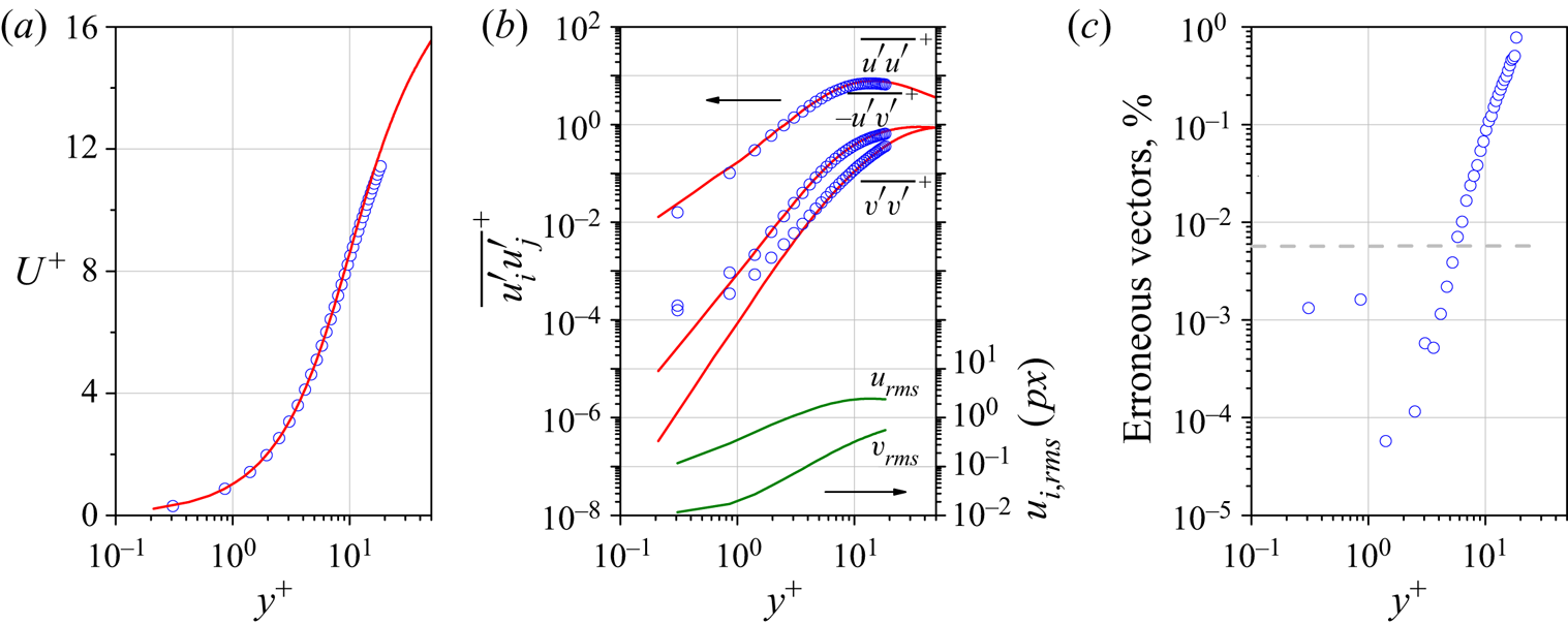
Figures 5(a) and 5(b) show the distribution of the time-averaged streamwise velocity  $U^{+}$ and correlations of velocity fluctuations
 $\overline {u'u'}^{+}$,
 $\overline {v'v'}^{+}$ and
 $\overline {u'v'}^{+}$ along
 $y^{+}$, which are in excellent agreement with our DNS results. Figure 5(b) shows the correlation profiles in log–log coordinates to inspect the accuracy of the employed technique. While for
 $\overline {u'u'}^{+}$ we observe a good collapse near the wall, but there is a small discrepancy for
 $\overline {v'v'}^{+}$ and
 $\overline {u'v'}^{+}$ for
 $y^{+}<4$. Recalculating
 $\overline {u'u'}^{+}$ and
 $\overline {v'v'}^{+}$ in
 $px$ units and expressing the corresponding root-mean-square values of both velocity components,
 $u_{rms}$ and
 $v_{rms}$, note that
 $v_{rms}$ is less than 0.1 px in the region of
 $y^{+}<4$ (see figure 5b). Thus, the wall-normal velocity fluctuations are of the order of random error generally resulting from PIV evaluation techniques. Nevertheless, the underresolution of
 $v'$ in the viscous sublayer does not affect further results and discussions.
Wall-normal profiles of (a) the time-averaged streamwise velocity, (b) the correlations of velocity fluctuations and (c) the number of erroneous velocity vectors detected by the median test (Westerweel & Scarano Reference Westerweel and Scarano2005). Solid lines on the bottom of figure (b) denote the root-mean-square of fluctuations of both velocity components to compare with the level of the measurement error. The horizontal dashed line in (c) indicates the measured probability of NWRFs.

As mentioned previously, there are certain measurement errors in the viscous sublayer. Their possible sources are PIV settings (interrogation window size, interrogation window overlap, etc.), image-processing method and experimental parameters (particle image density and diameter, image noise, etc.), yielding erroneous velocity vectors (Kähler, Scharnowski & Cierpka Reference Kähler, Scharnowski and Cierpka2012a,Reference Kähler, Scharnowski and Cierpkab). Extreme deviations of these vectors from the correct values can be detected by the median test discussed by Westerweel & Scarano (Reference Westerweel and Scarano2005). Figure 5(c) shows a fraction of erroneous vectors, which is significantly lower than the NWRFs probability in the viscous sublayer and less than  $1\,\%$ along the entire wall-normal distance, indicating high reliability of estimated velocity vectors. However, the measured data still includes random and bias errors (Raffel et al. Reference Raffel, Willert, Scarano, Kähler, Wereley and Kompenhans2018), which significantly affect the NWRF probability. For example, we consider a situation when experiments show negative streamwise velocity near the wall, which is comparable to the random error, i.e.
 $-u_{rms}< u<0$. Obviously, this will yield an incorrect impression of the NWRF probability and other statistical quantities. Thus, if the appropriate filtering procedure is not applied, eliminating the measurement error and preserving the real NWRF region, one can get a wrong impression about actual values of the spatiotemporal extension of NWRFs. An appropriate filtering procedure was applied in the present work with the detailed description presented elsewhere (Zaripov et al. Reference Zaripov, Li and Dushin2019). This allows us to exclude the frequency region where the measurement noise dominates. The following criterion was used for the cut-off frequency,
 $f_{cut}$:
 \begin{equation} \frac{\lvert\hat{U}(f_{cut})\rvert^{2}}{\lvert E \rvert^{2}} = 2, \end{equation}
where  $\hat {U}(f) = \mathscr {F}[\hat{u}(t)$] and
 $E(f) = \mathscr {F}[e(t)]$ represent continuous Fourier transform of measured fluctuating velocity components,
 $\hat {u}$ or
 $\hat {v}$, and random measurement error,
 $e$ respectively.
In experiments we detected eight NWRF events within the total time interval 7.18 in wall units at  $y^{+}=0.31$ during the whole video duration corresponding to
 $P = 0.0065\,\%$, which is slightly less than those presented in figure 4(a) for low Reynolds numbers. The mean geometrical characteristics of the NWRF regions are also slightly smaller in the vertical direction than expected (see figures 4b and 4c). This may be the result of random measurement errors, as already mentioned. Another possible reason affecting the experimental mean quantities is the data scarcity problem. According to Cardesa et al. (Reference Cardesa, Monty, Soria and Chong2019),
 $\Delta x^{+}$ ranges from 10 to 30, while
 $\Delta y^{+}$ concentrates around 1. Therefore, undersampling of the statistically analysed data, as in our experiments, will lead to a larger error in the mean estimation of
 $\Delta x^{+}$ than that of
 $\Delta y^{+}$. Another source of the underestimation is associated with the fact that in the case of planar PIV, as in the present work, three-dimensional events sliced by the light sheet produce smaller or larger outcome depending on the slicing position within the NWRF region, i.e. the edge or its middle part.
3. Results and discussion
The use of high-speed PIV allows us to analyse time signals of velocity within a field of view up to 19.7 wall units, over a sufficiently long period of time. This enables studying the near-wall flow region in great detail. The far-field flow region, not measured by PIV, is explored based solely on the DNS results.
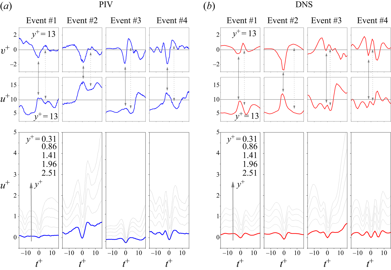
Figure 6 shows the time evolution of  $u^{+}$ and
 $v^{+}$ for different wall distances for typical NWRF events obtained both from PIV and DNS with maximum negative streamwise velocities centred at
 $t^{+}=0$. The streamwise velocity component exhibits pronounced deceleration zones for all considered distances from the wall. Taking into account that all these events are independent both in PIV and DNS featuring similar behaviour, we may speculate that the measurement error does not influence these data.
Time signals of the streamwise and wall-normal velocity components at various distances from the wall for four typical NWRF events from PIV (a) and DNS (b). Dark grey horizontal lines on top figures indicate time-averaged values of velocity components. The solid vertical arrows indicate the footprints of the so-called high-speed streaks while the dashed vertical arrows indicate low-speed streaks associated with near-wall vortical structures. The waveforms on the bottom figures are given for various distances  $y^{+}= 0.31$, 0.86, 1.41, 1.96 and 2.51 shown by the arrow corresponding to 4.5, 12.5, 20.5, 28.5 and 36.5 px for experiments in a viscous sublayer.

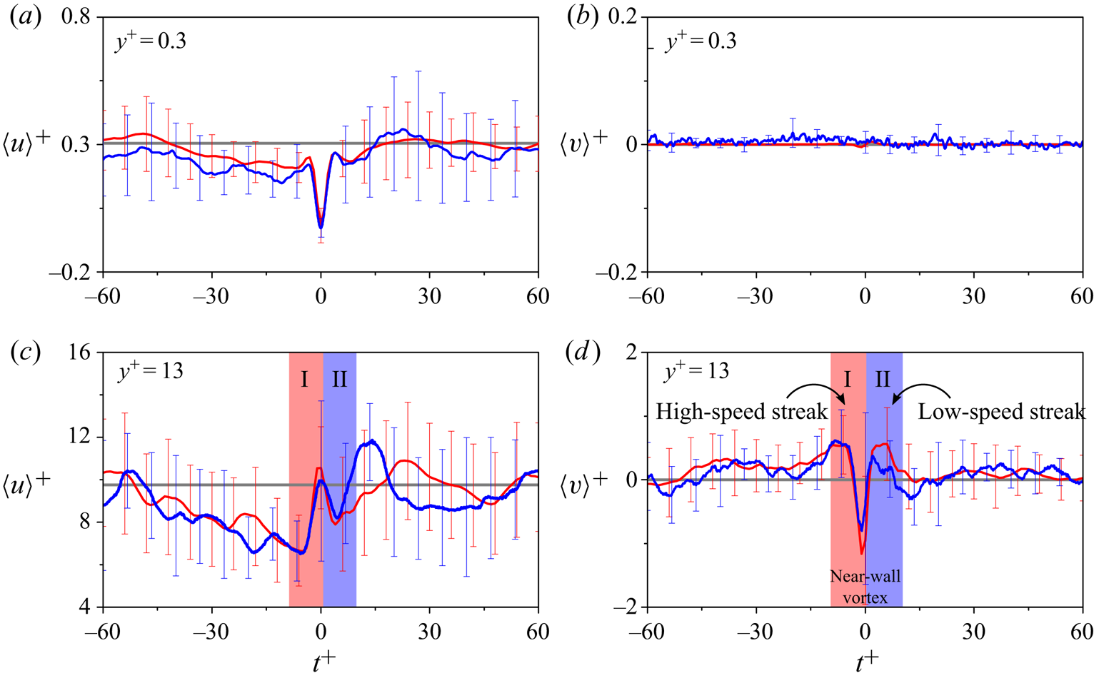
To get a statistical portrait of these events, we applied a conditional averaging procedure, which is further denoted as  $\langle \ldots \rangle$. This approach was also used by Chin et al. (Reference Chin, Monty, Chong and Marusic2018) and Cardesa et al. (Reference Cardesa, Monty, Soria and Chong2014, Reference Cardesa, Monty, Soria and Chong2019), who mainly considered a flow domain in close proximity to the NWRF region and downstream, although the flow domain upstream of NWRFs seems equally important in terms of understanding the mechanism of the NWRF formation. We start with the conditional averaging of the time series shown in figure 7, demonstrating
 $\langle u \rangle ^{+}$ and
 $\langle v \rangle ^{+}$ at
 $y^{+}=0.3$ and 13, similar to figure 6. The comparison of PIV and DNS signals demonstrates a striking agreement. One can distinguish alternating zones of downward (zone I) and upward (zone II) flow motions belonging to either quasi-streamwise or transverse vortical structure generally located in the buffer region. Within zones I and II, the conditional averages of
 $\langle u \rangle ^{+}$ and
 $\langle v \rangle ^{+}$ are slightly lower than time-averaged values, indicating that NWRFs occur in the fluid region affected by the L-M flow structure. More specifically, NWRFs typically occur at the tail of the large-scale L-M flow region observed in the time interval of
 $-50< t^{+}<0$, roughly corresponding to
 $-500< x^{+}<0$ interval with a convective velocity
 $\langle U\rangle ^{+} \approx 10$ at
 $y^{+}=13$. This fact somewhat contradicts the observations of Bross et al. (Reference Bross, Fuchs and Kähler2019), who found that NWRFs appear along the entire area of the L-M flow region. Their database was obtained for an APG configuration with a discrepancy possibly coming from an overall deceleration of the flow with the near-wall coherent vortical structures causing stronger NWRFs. In ZPG TBL or channel flow, the flow deceleration inherent in the L-M flow region is not sufficiently strong, thus an additional effort is required to cause a flow reversal. Cardesa et al. (Reference Cardesa, Monty, Soria and Chong2014) and Chin et al. (Reference Chin, Monty, Chong and Marusic2018) showed that this effect can be attributed to a strong motion towards the wall, directly above the NWRF region. As shown subsequently, such a flow motion pressing the near-wall vortical structure against the wall belongs to a large-scale H-M flow region, which generates the vortex itself near the wall (see figures 8(a) and 9, as well as the corresponding discussion).
Time signals of streamwise (a,c) and wall-normal (b,d) velocity components averaged over 158 and 8 NWRF events detected by DNS and PIV, respectively. Error bars represent the root-mean-square of the corresponding values. Thick red waveforms correspond to the data obtained by DNS, blue waveforms correspond to the experimental data. Dark grey horizontal lines indicate time-averaged values of velocity components.

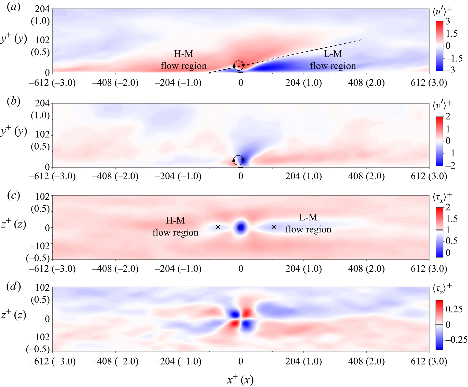
Conditionally averaged (a) streamwise, (b) wall-normal components of velocity fluctuations, and (c) streamwise, (d) spanwise components of the wall shear stress. Flow is from left to right. Black rectangles located at  $(x^{+},y^{+}) = (0, 0)$ in (a,b) bound the NWRF regions. The dashed line in (a) illustrates the interface between L-M and H-M flow regions and has a slope of
 $13^{\circ }$. Crosses in (c) indicate coordinates of minimum points of the streamwise component of the averaged wall shear stress. The black contour in (c) indicates the region of the averaged NWRF event. Thick ticks on the colour bars indicate the mean values of the corresponding variables.

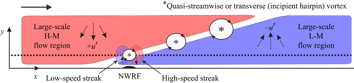
The  $x - y$ plane of a schematic diagram of the flow pattern explaining the mechanism of the NWRF formation.

Figure 8 shows conditionally averaged fields of velocity fluctuations and wall shear stress in the  $x - y$ and
 $x - z$ planes. The fields in the vertical plane shown in figures 8(a) and 8(b) demonstrate that the NWRF is accompanied by a zone of strong flow motion towards the wall located in the buffer region and characterised by higher streamwise momentum, followed by an upward motion with lower streamwise momentum. This is a typical picture for both the oblique quasi-streamwise and transverse vortices. However, the average size in wall units is of the order of 50, which is closer to the characteristics of the transverse vortices (
 ${\sim }50$) rather than quasi-streamwise vortices (
 ${\sim }25$), see Robinson (Reference Robinson1992), indirectly indicating that NWRFs are probably formed by transverse vortices. Nevertheless, the important role of quasi-streamwise vortices in the formation of NWRFs should not be excluded and may be re-examined in light of previous publications (Lenaers et al. Reference Lenaers, Li, Brethouwer, Schlatter and Örlü2012; Cardesa et al. Reference Cardesa, Monty, Soria and Chong2014; Brücker Reference Brücker2015; Vinuesa et al. Reference Vinuesa, Örlü and Schlatter2017; Bross et al. Reference Bross, Fuchs and Kähler2019).
In a similar manner to the observations of Chin et al. (Reference Chin, Monty, Chong and Marusic2018) and Cardesa et al. (Reference Cardesa, Monty, Soria and Chong2014, Reference Cardesa, Monty, Soria and Chong2019), there is a large-scale L-M flow region downstream of the NWRF event (see figures 8a and 8c). The spatial extent of this flow region is in good agreement with the value observed in figure 7 for conditionally averaged time signals. However, to the best of our knowledge, there is no mention of a large-scale H-M flow region upstream of the NWRF occupying a large flow domain and originating in the near-wall region at a distance of about  $x^{+} = 700$ upstream, which also extends around
 $x^{+} = 300$ downstream of the NWRF region. This fact explains the observation of Lenaers et al. (Reference Lenaers, Li, Brethouwer, Schlatter and Örlü2012) that most of the NWRF events occur below large-scale H-M flow regions. At the same time, a large-scale L-M flow region can also be observed above the NWRF regions although less often, confirming the results of Lenaers et al. (Reference Lenaers, Li, Brethouwer, Schlatter and Örlü2012).
We observe an interaction of large-scale L-M and H-M flow regions through the interface between them. According to a widely accepted mechanism of the near-wall turbulence production (Robinson Reference Robinson1991), this kind of interaction leads to a strong shear layer at the interface developing into the near-wall transverse vortices, followed by hairpin vortices owing to the shear-layer instability as schematically demonstrated in figure 9. Figures 8(a) and 8(b), although demonstrating averaged velocity fields, capture vortical structures causing the NWRF at the interface between the L-M and H-M flow regions. However, according to Robinson (Reference Robinson1991), one would expect a train of hairpin vortices that, unfortunately, cannot be captured by averaged fields owing to the blurring effect of different spatiotemporal scales of vortices growing with distance from the wall.
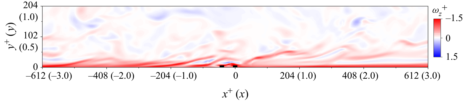
Figure 10 shows an instantaneous vorticity field in the  $x - y$ plane associated with two subsequent NWRF events clearly demonstrating the existence of the vortical structure located directly above the NWRF region representing a group of hairpin-like vortices. This situation is not unique and represents a statistically common situation supported by the fact that two additional local minima at
 $x^{+} \approx -75$ and 110 have been detected in the conditionally averaged field of streamwise wall shear stress shown in figure 8(c). Figure 6 also supports this scenario both numerically and experimentally, demonstrating a wavy time signal at different
 $y^{+}$ indicating multiple alternations of flow deceleration zones in the viscous sublayer. A time interval between these local minima associated with deceleration zones varies between
 $t^{+} = 5$ and
 $10$. Taking into account a convective velocity of vortices in the buffer region, vortical structures causing near-wall flow decelerations, including the NWRF events, are located from each other at a distance between
 $x^{+} = 50$ to
 $100$. Thus, the basic principle in this scenario is that a typical train of vortices does not systematically lead to subsequent NWRF, however, they contribute to the conditionally averaged fields as shown in figure 8, explaining multiple minima of the wall shear stress field.
An instantaneous field of spanwise component of vorticity  $\omega ^{+}_z$. Black squares located at
 $(x^{+}, y^{+}) = (0, 0)$ and
 $(x^{+}, y^{+}) = (-60, 0)$ bound the NWRF regions.

4. Conclusions
We have studied the NWRF phenomenon in a fully developed turbulent duct flow using DNS and PIV, at relatively low Reynolds number  $Re_\tau \simeq 200$ both featuring high spatiotemporal resolution. The time-averaged statistics were validated against data from the literature. A striking agreement between conditional averaged time signals around NWRF events obtained from DNS and PIV was demonstrated. To the best of our knowledge, this was the first experimental observation of NWRFs at such a low Reynolds number. In addition to the two generation mechanisms proposed by Bross et al. (Reference Bross, Fuchs and Kähler2019), which relate the generation of the NWRF events with L-M flow structures, our analysis revealed large-scale H-M flow regions upstream of NWRFs leading to a common interface between H-M and L-M zones. This interface stimulates the growth of hydrodynamic instabilities in a strong shear layer resulting in a train of hairpin vortices with the closest to the wall being responsible for NWRF formation. The incipient hairpin vortex and the NWRF event tend to occur at the tail of the L-M flow region, where strong downward flow pushes the vortical structure to the wall. The similarity of the flow topology downstream of the NWRF region for the present Reynolds number
 $Re_\tau \simeq 200$ with those for
 $Re_\tau = 1000$ (Chin et al. Reference Chin, Monty, Chong and Marusic2018) and
 $550 \leqslant Re_\tau \leqslant 2000$ (Cardesa et al. Reference Cardesa, Monty, Soria and Chong2019) suggests the generality of the proposed mechanism. However, we could not observe the mechanisms outlined by Bross et al. (Reference Bross, Fuchs and Kähler2019) possibly owing to somewhat different flow conditions, including the pressure gradient.
We have shown the possibility of two subsequent NWRF events. A visual inspection of the instantaneous flow fields associated with these events demonstrates the involvement of two successive vortical structures located directly above the NWRF regions and included in a group of hairpin-like vortices coming one after another. This kind of arrangement modulates the streamwise and wall-normal velocity components leading to multiple alternations of decelerated and accelerated flow regions near the wall in the streamwise direction. However, most of the flow regions decelerated in such a manner do not exhibit reverse flows near the wall as the flow regions, which potentially could lead to NWRF events, are not sufficiently retarded in the buffer region and log-law region (Kim & Hussain Reference Kim and Hussain1993). The proposed mechanism of the NWRF formation explains two local minimum points observed downstream and upstream of the NWRF event in the averaged field of the streamwise component of the wall shear stress.
Funding
Experiments were conducted within the Russian Science Foundation grant no. 19-19-00355. Numerical simulations and data analysis were conducted within the Russian Science Foundation grant no. 19-79-30075. The development of the numerical code was supported by the state contract with IT SB RAS. The computational resources were provided by the Joint Supercomputer Center of the Russian Academy of Sciences, Moscow.
Declaration of interests
The authors report no conflict of interest.