1 Introduction
Human beings can easily imagine what a ‘long spoon’ looks like. The creation of this visualization requires an enormous amount of information—much more than the information in the two-word phrase that triggers it. How do reasoners generate this information from an input containing so little? We begin to answer this question in this paper.
Specifically, we will show how a reasoner could estimate the quantitative meaning of qualitative adjectives such as ‘big’ and qualitative prepositions such as ‘beside’. For example, if the reasoner is asked visualize a ‘big leopard’, exactly how big should that leopard be? If asked to imagine ‘a keyboard beside a mouse’, how far would they be from each other?
We implemented our theory in an operational Python computer program, called Visuo. The program takes as input a set of labels, such as ‘long rug’, or ‘big flag over a small lawn’. In a process we call ‘visuospatial instantiation’, the program outputs symbolic scene descriptions that include quantitative magnitudes based on input adjectives and prepositions.
We will describe our theory of visuospatial instantiation, Visuo (the program written to test the theory), and its evaluation.
1.1 Theory overview
Since the task of visual imagination is complex, our research provides an explanation of a small part of this process: how quantitative information about nouns, adjectives, and prepositions is stored and then used to estimate new quantitative information, when triggered by a qualitative stimulus.
The meanings of adjectives and prepositions in natural language are not absolute, but relative to the objects being described. For example, a hand ‘over’ a stove is much closer than a cloud ‘over’ a lake. A large dog is far smaller than a large nation. We suggest that reasoners retrieve and modify appropriate memories when possible. For example, if asked to visualize a ‘large raven’, and if there are descriptions in memory of a large ravens, the large raven prototype will be retrieved and used for visualization. But when a match is not found, the reasoner infers the meaning of the adjectives and prepositions by analogy, transferring from better-known concepts in memory, such as ‘crow’.
Our theory includes two phases: the training phase, when experienced visuospatial stimuli are incorporated into memory, and the visualization phase, when, given some input to visualize, information in memory is used to create a description of a new, imagined visual scene.
Reasoners experience visual stimuli in the world, and often these stimuli are labeled. For example, a reasoner might see an object associated with a label such as ‘crow’. A different stimulus might be labeled as a ‘large crow’, or ‘small city’. Suppose a reasoner has experienced many crows, many of which were labeled with different qualitative size descriptors, such as ‘tiny’, ‘small’, ‘large’, and ‘huge’. Let us also suppose the reasoner has experienced many instances of ravens, which are associated with the ‘raven’ label but not with qualitative size labels. When asked to imagine a large raven, since the reasoner has not experienced a raven that was labeled as ‘large’, it must infer a meaning of ‘large’ from some other concept in memory. According to our theory, a reasoner in this situation transfers the notion of ‘large’ from a semantically related concept, such as ‘crow’, rather than a less-related concept, such as ‘city’. With a notion of ‘large’ from a related concept, the reasoner can make a reasonable guess as to how large a ‘large raven’ would be. This informs the final visualized image description.
In the training phase, Visuo takes as input a file describing visuospatial experiences. Its outputs are changes to its memory. In the visualization phase, Visuo takes as input a phrase describing what is to be visualized. The output is a propositional scene description including quantitative magnitudes.
The theory is both a model of human cognition and a contribution to artificial intelligence (AI). As such, when we write that a ‘reasoner’ does x, we mean to say we hypothesize AI reasoners should do x, and that human reasoners actually do x.
2 Training phase
2.1 Input for training phase
Theory. Reasoners encode many aspects of incoming visual quantitative information. We will focus on those aspects we conjecture are relevant to our particular task of visual imagination.
Reasoners pull out three aspects from each episode of experience, or scene: a label, attributes, and quantitative values. The kinds of input our theory endeavors to understand (in both the training and visualization phases) includes the following kinds of example inputs:
[raven]
[large raven]
[bright [long [large raven]]]
[[raven] above [tall tree]]
[[thin raven] above [tall tree]]
[[bright [long [large raven]]] above [tall tree]]
These examples are instances of a generalized recursive grammar:
NP -> [N]
NP -> [Adj NP]
S -> [NP (Prep NP)]
where S is an input string (simplified sentence), N is a noun, NP is a noun phrase, Adj is an adjective, and Prep is a preposition.
In the training phase, each preposition and noun in the input is associated with some set of attributes. For example, a ‘large crow'might be associated with a certain size and possibly other attributes as well, such as length. In the example of a ‘large crow above tree’, an attribute associated with ‘large’ might be ‘size’ and an attribute associated with ‘above’ might be ‘distance’.
Each attribute (associated with each noun and preposition) is associated with a value. The value represents the real-world magnitude of that attribute, in that visual scene. Each preposition and noun is associated with one or more attributes, and each of those attributes is associated with a single numerical value.
Reasoners add this information to episodic memory, and then create or modify appropriate parts of semantic memory.
Implementation. Our implementation of the theory is a Python computer program called Visuo, which takes a file as input for the training phase and a text string for the visualization phase.
The training phase input file contains entries representing aspects of visual scenes. The labels, attributes, and values are represented as follows:

These values are measured in arbitrary mental units rather than more objective metrics such as centimeters or kilograms. So a crow that is 40 cm long might get a ‘size’ value of ‘10’ in these mental units. This is based on the notion that a person need not know any particular culturally invented unit of measure to represent visuospatial magnitudes.
In example 1, the ‘crow’ has two attributes associated with it: size and length. In Example 2, the distance describes only the ‘aboveness’ of the large bat in relation to the forest.
The parser reads the input file, and transforms each input example into an exemplar in memory, which contain all the characteristics of the example. Exemplars, which we will explain in detail in the next section, are representations of individual experiences. Additionally, the parser identifiers each word as a noun, adjective, or a preposition.
For example, ‘large bat’ and all exemplars created from this phrase acquire the attribute size, with an attribute value of 12 (we will describe below how these values are not stored as exact numbers, but as a distribution containing the attribute value's degrees of membership in each fuzzy number set).
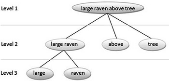
There are two methods the parser uses to create exemplars out of the input phrase (see Figure 1). If the input phrase has a preposition in it, the first method is used, which parses the phrase into two exemplars. The first exemplar is that of the entire phrase, and the second exemplar is one containing only the preposition. For example, ‘[[large bat] above [tree]]’ would be parsed into an exemplar ‘large bat above tree’, and also into an exemplar ‘above’. The first would be an exemplar of how ‘above’ relates to a bat and a tree, and the second would be a general exemplar of ‘above’ as a generic term.
Result of parsing Example 2 from the input file above. Each node is turned into an exemplar

Noun phrases use the second method. The phrase is parsed with a depth-first recursive method, and each segmentation is used to create a new exemplar. The very first exemplar is created from the entire input phrase. The remaining is recursively broken down into sub-phrases, where each sub-phrase is either a word, or a grouping of words as grouped by square brackets. If a sub-phrase contains only one word, then the parser does not attempt to break it down further. If the sub-phrase contains multiple words, or bracketed words, then that chunk is further broken down.
For example, the input phrase ‘[large bat]’ would produce three exemplars. Visuo would first create an exemplar for ‘large bat’. Since the ‘large bat’ contains more than one word, it would further be broken down into an exemplar for ‘large’, then one for ‘bat’. Since the previous phrase cannot be recursively broken down further, no more exemplars are created for this input phrase. The process above is the same no matter how many attributes are associated with a particular name.
2.2 Creation of exemplars in episodic memory
Exemplars represent memories of objects occurring at a specific place and time (Tulving, Reference Tulving1984). For example, when the reasoner takes as input a crow of size ‘10’, that information is stored in an exemplar.
2.2.1 Distributions of fuzzy set membership
Theory. We propose that AIs should not (and people do not) exactly represent magnitudes gleaned from perception. Rather, the memory representations should account for perceptual uncertainty and vagueness. Furthermore, it should be reduced in dimensionality to increase ability to generalize. Spatial receptors in the retina and the visual system of the brain have receptive regions that have varying sensitivity to different attributes, such as the different orientations of an edge (Hubel & Wiesel, Reference Hubel and Wiesel1965). In fact, detectors have been found to pick up even high order visual concepts such as buildings and faces (Perret et al., Reference Perret, Hietanen, Oram and Benson1992; Tanaka, Reference Tanaka1993; Kreiman et al., Reference Kreiman, Koch and Fried2000a, Reference Kreiman, Koch and Fried2000b). Also, behavioral data show that people represent things with graded membership to categories in general (Hampton, Reference Hampton2007), so we conjecture that higher-level perceptual detectors in the brain also represent spatial magnitudes and detect relevant stimuli with variable category membership as a function of the firing rates of neural populations. In our theory, fuzzy set memberships (Zadeh, Reference Zadeh1965) represent these differential firing rates. In fuzzy set theory, the membership of an instance in a given set is described with a fuzzy membership value ranging from 0 (clearly not in the set) to 1 (clearly a member of the set).
For an example relevant to our task, an input of ‘10’ mental units could represent a magnitude in the real world of, say, 5′8″, with varying degrees of certainty and vagueness. In this example, the input number 10 becomes a fuzzy number (Dubois & Prade, Reference Dubois and Prade1987). As opposed to ‘crisp’ numbers, fuzzy numbers are numbers that have a fuzzy range of values. Each in itself is a fuzzy set. The fuzzy number 5 is the fuzzy set of all magnitudes of numbers close to 5. A crisp magnitude of 6 is somewhatin the set of fuzzy 5 magnitudes. An input number is a member of all fuzzy number sets to some degree, represented by a number between 0 and 1. An input of ‘10’, for example, would have a 1.0 membership in the fuzzy number 10 and only a 0.6667 membership in the fuzzy number 5.
In our theory, the detectors for magnitude have overlapping ranges of sensitivity (varying receptive fields). Input numbers are decomposed into the fuzzy set of magnitudes. Without this decomposition the prototype memory requirements would increase linearly with increasing examples. With the existence of the decomposition, prototype memory requirements are constant. This reduction in dimensionality can become considerable as the number of examples becomes large. This is our account of why humans often have general ideas of how large known objects are, but typically cannot recall every object they have ever seen. Decomposition of stimuli is not uncommon in the brain. For example, simple cells in the striate cortex appear to act as a Gabor wavelet to decompose stimuli in the spatial domain into a reduced representation in the frequency domain (Pollen & Ronner, Reference Pollen and Ronner1981; Daugman, Reference Daugman1985; Jones & Palmer, Reference Jones and Palmer1987).
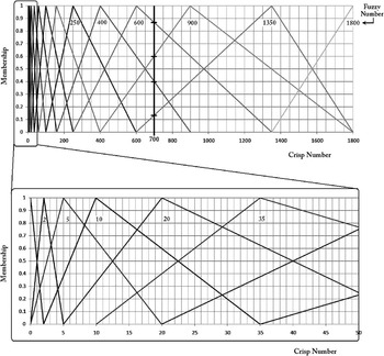
Implementation. Our collection of magnitude detectors is modeled by a distribution that has a slot for 15 points on a logarithmic mental unit scale (0, 2, 5, 10, 20, 35, 65, 100, 160, 250, 400, 600, 900, 1350, 1800)Footnote 1. It is represented logarithmically because there is evidence showing that people represent distances logarithmically (Dehaene et al., Reference Dehaene, Izard, Spelke and Pica2008). The distribution itself is a list of numbers representing the membership of the crisp input value in fuzzy all the fuzzy number sets. These fuzzy numbers have overlapping ranges, just as spatial detectors do (see Figure 2).
Fuzzy numbers and their actual membership functions at two different scales. The values along the horizontal axis represent crisp number inputs. The values along the top label are the fuzzy number sets. The vertical axis represents the degree of membership of that crisp number in a given set. For example, a crisp input of 700 is a member of fuzzy number 400 to a degree of 0.40, a member of fuzzy number 600 to a degree of 0.8667, a member of fuzzy number 900 to degree 0.60, a member of fuzzy number 1350 to degree 0.1333 and a member of all other fuzzy numbers to degree 0.0

For example, suppose the reasoner views a crow of size 10 (in mental units). The distribution to represent this would contain the following information:
(0.0, 0.0, 0.6667, 1.00, 0.3333, 0.0, …) [crow1 size]
Each number in the distribution is a membership of the crisp input number (in this case ‘10’) for each point on the mental unit line (0, 2, 5, 10, 20, 35, etc.). This process of turning a crisp number into fuzzy memberships is called ‘fuzzification’ (Negnevitsky, Reference Negnevitsky2005). An input of ‘10’ overlaps with nearby fuzzy numbers ‘5’ and ‘20’, resulting in the distribution above. ‘10’ does not overlap with the fuzzy number ‘2’, so its membership for that slot is 0.0. In the next section, we describe the details of how our program fuzzifies crisp inputs.
Each of these distributions is associated with an attribute, and also with either a preposition or a noun. A particular noun phrase can have multiple exemplars, each with its own distribution—one for each attribute. In the example 1 above, the ‘large crow’ exemplar would create a distribution for ‘size’ and for ‘brightness’.
We hold that the mental units are represented (roughly) logarithmically, but we do not know, in human beings, exactly what numbers are on the scale nor how real-world magnitudes translate to these mental units. Thus, the specific numbers we use in the program are arbitrary, but we believe that this does not affect the functional nature of the theory nor the abilities of the program. That is, we do not believe that a different set of logarithmically organized numbers would change the program's behavior in a way relevant to our hypotheses.
2.2.2 Fuzzification
The program transforms a crisp number N into a distribution of the form {u1:S1, u2:S2,…, un:Sn}, where ui is the membership of N in a given fuzzy set Si. More specifically, each Si is a fuzzy number, which is a continuous normalized fuzzy set where the membership of the set is 1.0 only at one element (see Figure 2). Fuzzy sets have overlapping ranges. The distribution is created by fuzzifying the ‘crisp’ number N into each fuzzy set Si, and storing the associated membership ui. In order to avoid confusion between crisp numbers and fuzzy number sets, all crisp numbers will be appended with a ‘C’ (e.g. 100C) and all fuzzy number sets will be appended with an ‘F’ (e.g. 100F)Footnote 2.
The complete list of fuzzy numbers used in the program is {0F, 2F, 5F, 10F, 20F, 35F, 65F, 100F, 160F, 250F, 400F, 600F, 900F, 1350F, 1800F}. For the most part, each fuzzy number overlaps with three numbers to the right and three to the left of it. For example, the membership function for the crisp number 100C would linearly increase from 0.0 to 1.0 for the fuzzy numbers 35F and 100F and linearly decrease from 1.0 to 0.0 for fuzzy numbers 100F to 250F, respectively. A crisp number 35C or 250C would have a membership of 0.0 in the fuzzy number 100F. A crisp number 100C would have a membership of 1.0 in the fuzzy number 100F. Any value in between 35C and 100C or 100C and 250C would have a membership u determined by linear interpolation
 $$u\,{\rm{ = }}\,\left( {{{u}_a}\,{\rm{ + }}\,\frac{{{\rm{(}}N\,{\rm{ - }}\,{{N}_a}{\rm{)}}\,\times \,({{u}_b}\,{\rm{ - }}\,{{u}_a})}}{{{{N}_b}\,{\rm{ - }}\,{{N}_a}}}} \right)$$
where ua is the membership of Na and ub is the membership of Nb.
Any quantitative number <35C or >250C would have a membership of 0.0 in a fuzzy number 100F as it is outside the range.
To create the fuzzy distribution from input N, the model iterates through each fuzzy number and fuzzifies N with respect to that number, resulting in a distribution of the form {u0:S0, u1:S1, u2:S2,…, un:Sn}. The crisp number N has been transformed into what we believe is a realistic mental representation. For example, the distribution of 175C would be:
{0.0 : 0F, 0.0 : 2F, 0.0 : 5F, 0.0 : 10F, 0.0 : 20F, 0.0 : 35F,
0.0 : 65F, 0.5 : 100F, 0.9375 : 160F, 0.5 : 250F, 0.0625 : 400F,
0.0 : 600F, 0.0 : 900F, 0.0 : 1350F, 0.0 : 1800F}
For the remainder of the paper, the numbers indicating fuzzy sets (i.e. the part after the colon) will be not shown but implied.
2.2.3 Exemplars
Theory. In this theory, each exemplar contains some number of distributions, as described above. The example of [[large crow] over [thick tree]] is parsed. Reasoners create exemplars for each node in the tree shown in Figure 1: large crow, large, crow, large crow over thick tree, over, thick tree, thick, and tree. Each of these exemplars will have one distribution for every attribute that is associated with it in the input.
Implementation. From the training input phrase [[large crow] over [thick tree]], where the ‘large crow’ has a size = 10, and the ‘large crow over thick tree’ has a distance = 10, and the ‘thick tree’ has a thickness = 2, Visuo creates the following exemplars, using the fuzzification process described above:
[large1 crow1] size [0.0, 0.0, 0.0, 0.2, 0.75, 0.8, 0.25, 0.0, …]
[large1] size [0.0, 0.0, 0.0, 0.2, 0.75, 0.8, 0.25, 0.0, …]
[crow1] size [0.0, 0.0, 0.0, 0.2, 0.75, 0.8, 0.25, 0.0, …]
[[large1 crow1] over1 [thick1 tree1]] distance [0.0, 0.0, 0.0, 0.0, 0.0, 0.0, 0.6, 1.0, 0.4, 0.0, …]
[over1] distance [0.0, 0.0, 0.0, 0.0, 0.0, 0.0, 0.6, 1.0, 0.4, 0.0, …]
[thick1 tree1] thickness [0.0, 0.0, 0.0, 0.0, 0.25, 0.769, 0.75, 0.231, 0.0, …]
[thick1] thickness [0.0, 0.0, 0.0, 0.0, 0.25, 0.769, 0.75, 0.231, 0.0, …]
[tree1] thickness [0.0, 0.0, 0.0, 0.0, 0.25, 0.769, 0.75, 0.231, 0.0, …]
There is a numeral ‘1’ after the items so that the names have unique symbols. Though the input might be ‘crow’ every time, each exemplar is stored as ‘crow1’, ‘crow2’, etc., to differentiate the instances perceived.
2.3 Prototypes in semantic memory
Theory. In our theory, semantic memory consists of prototypes. Inspired by Rosch (Reference Rosch1973), they are memories of general concepts of things, abstracted from specific instances. They represent the family resemblance of a category. For quantitative attributes this is often interpreted as mean values. We call this part of memory ‘semantic’ because it represents the meaning of words. The first time Visuo experiences a crow's size, it creates a prototype for crow size. For each subsequent experience of a crow, it modifies the crow size prototype, even as it creates new exemplars for each experience.
Suppose the reasoner experiences ([large crow] size = 10). The reasoner creates a distribution for the prototype of ‘large crow’, containing all of the information from its exemplar, plus a count of the number of examples experienced so far with this label (for the first instance of ‘large crow’, the number of instances seen would be, of course, one). As the crisp input number is stored as a distribution over fuzzy number sets, it differs from more traditional prototypes, which store exact means.
[large1 crow1] size (0.0, 0.0, 0.0, 0.2, 0.75, 0.8, 0.25, 0.0, …) [examples:1]
Upon experiencing another large crow, each fuzzy membership number  $$\[--><$>{{v}_{{\rm{avg}}}}<$><!--$$
in the distribution is averaged with
 $${{v}_{{\rm{avg}}}}\, = \,\frac{{(n\,\times \,{{v}_{{\rm{old}}}})\, + \,{{v}_{{\rm{new}}}}}}{{n\, + \,{\rm{1}}}}$$
where v old is the previous value, v new is the new value. Following the calculation of v avg, the count n is increased by 1. The reasoner incorporates each new experience of the same category into the prototype. For each point in the mental unit scale, the prototype represents the mean value of the memberships all exemplars for the corresponding fuzzy number. In this way, the prototype represents an average of all experiences.
Like the exemplars, prototypes also keep separate records for each attribute, containing a distribution and a count of experienced examples. So if a ‘large raven’ has a size and a length, the prototype would contain a distribution for each. This also happens for attributes that might be thought to be irrelevant to an adjective, such as ‘large’. For example, an experienced ‘large crow’ might have a ‘size’ and a ‘brightness’ (indicating how dark it is). Though one would not think that the largeness of the crow describes the brightness, the prototype stores it. This allows Visuo to pick up on implicit correlations in the environment. For example, very small chickens are yellow, but when they grow older they are not (chicks are yellow). This is true even though ‘very small’ is not used to describe any aspect of color.
Note that there is also a prototype created for ‘large size’. This is a representation of largeness that is independent of what objects have actually been seen (e.g. crows, tuna sandwiches). It is the reasoner's generic representation of ‘large’.
Similarly prototypes are created or modified for each distribution in the exemplar.
As this processing is relatively straightforward, we will not describe our implementation of the creation of prototypes.
3 Visualization phase
Above we described the training phase, how a reasoner collects and represents observations conducted before the task of visualization starts. The specific task we are describing in this paper is to estimate a quantitative magnitude from a qualitative (verbal) stimulus. For example, if the reasoner is asked to imagine a ‘large crow’ (the ‘visualization stimulus’), how can the reasoner use memories of crows to effectively guess how large this imagined crow should actually be? If asked to imagine a ‘large raven’, how can the reasoner use memories of crows to make an estimate of the raven's actual size? These are the kinds of tasks typical of the visualization phase.
We conjecture that using context affects the outputs, making them more psychologically realistic. By context we mean both the context of the other things in memory (e.g. the crows and ravens you have seen before), as well as the context in the visualization stimulus (i.e. the other words in the input).
At a high level, the reasoner takes the visualization stimulus and tries to find a matching prototype in semantic memory. If it is found, then the information in that prototype is de-fuzzified and output (de-fuzzification is described in detail below). For example, if asked to imagine a ‘large crow’, and the reasoner has a prototype for large crows, then the reasoner will de-fuzzify the distribution for the prototype of large crows and output the resulting crisp number as the size of the imagined crow. This is the trivial case.
The more interesting case is when there is not an exact match found in semantic memory. When this happens, the reasoner breaks the visualization stimulus into smaller pieces, recursively, until either matches are found, or the input cannot be further broken down (see Figure 3).
Tree representation of a visualization stimulus [[large raven] above [tree]].

For example, suppose the visualization stimulus is ‘[large raven] above tree’. The reasoner will search its semantic memory for prototypes describing the entire stimulus [[large raven] above [tree]]. Suppose the reasoner has not experienced a scene labeled this way. The reasoner parses the input and then searches for prototypes describing the first node [large raven]. If that fails, the reasoner searches for prototypes for ‘large’ and for ‘raven’.
Specifically, the reasoner searches for the distribution of ‘large’ that most closely matches ‘raven’. For example, suppose the only prototypes for ‘large’ in semantic memory are for crows, cities, and the generic concept of ‘large’. The reasoner will use a distribution of ‘large’ for the most semantically related concept. In this case, it would be ‘large crow’. The information in the ‘large crow’ distribution is transferred and adapted to the new ‘large raven’ distribution. The details of this process are in Sections 3.2 and 3.2.3. With the creation of this new distribution, the reasoner now has an exact match for ‘large crow’, which it has been searching for.
This is conceptually combined with ‘above’ and ‘tree’, finally creating a new exemplar and prototype for [[large raven] above [tree]]. With this final prototype created, the reasoner can de-fuzzify the prototype (as in the trivial case), and the reasoner outputs a number for how large the large raven is, and how far above the tree the large raven is.
We will now describe the processes of retrieval, conceptual combination, transfer, and de-fuzzification.
3.1 Retrieval: searching for prototypes in semantic memory
The system depth-first searches the parse tree, looking for matches for each node in semantic memory. If the node represents a phrase containing a compound term (e.g. ‘large raven’, as opposed to a single term, such as ‘raven’) then Visuo will only match to prototypes in memory for which there is an exact match on the that phrase. If the compound term is not found, then the children nodes are searched. This process continues until the terms are found. At this point, Visuo combines the prototypes through conceptual combination (Section 3.2).
We will explain this with the example. The task is to visualize ‘[[large raven] above [tree]]’. The parse tree is created, as shown in Figure 1. There is no exact match in semantic memory for the root node, as this specific concept has not yet been experienced. Visuo shifts from looking at the node of level 1 to the nodes of level 2, starting with ‘large raven’. The prototypes are searched, but since a ‘large raven’ has never been experienced, there is not yet a prototype for it, so no match is found. The children of the ‘large raven’ node are searched next (level 3). The first node, ‘large’, is searched and a prototype of large is found and returned. The next child node ‘raven’ is also found as a concept, since examples of ravens have been seen. Since all prototypes for each child node of ‘large raven’ have been found, Visuo will attempt to perform conceptual combination on the prototypes ‘large’ and ‘raven’ to create a novel prototype of ‘large raven’ (this is discussed in the next section). Following the creation of ‘large raven’ and the retrieval of ‘over’ and ‘tree’, conceptual combination is performed to create a prototype for ‘[large raven] above [tree]]’.
3.2 Conceptual combination
Conceptual combination is the process of combining ideas together to create a new idea. There are two methods used in this paper, one for the merger of an adjective with a noun phrase, and one for combining two noun phrases with a preposition.
An adjective is combined with a noun phrase by disambiguating the sense of the adjective (Section 3.2.1), understanding how the adjective modifies similar concepts through the creation of a concept modifier (Section 3.2.2), and finally, merging the adjective and noun such that the relevant properties are transferred (Section 3.2.3). For example, to transfer the concept of ‘tall’ from building to house, Visuo figures out how to transform the distribution of ‘building’ to ‘tall’ building, and applies the same transformation to ‘house’.
Noun phrases are merged with a preposition by disambiguating the sense of the preposition (Section 3.2.1). Though this has not yet been implemented in Visuo, our theory holds that the case where the preposition is modified by an adverb (e.g. ‘far above’) is accomplished as described in Sections 3.2.2 and 3.2.3.
3.2.1 Word sense disambiguation
Theory. The first step in conceptual combination is to correctly identify the sense of the words to be combined. For example, the sizes associated with a ‘large’ mouse are smaller than those of a ‘large’ airplane. This is accomplished by searching memory for semantically related concepts. We conjecture that reasoners do this because it is more likely that similar semantic meanings predict similar contexts, and that similar contexts will use similar senses of words.
Implementation. Visuo searches for adjectives and prepositions within the context of the nouns (or noun phrases). We will describe searches for adjectives first, by following through an example.
If Visuo is searching for a sense of ‘large’ that is relevant to a ‘raven’, the first step is to retrieve from memory all prototypes that contain the word large and pair them with the generic version of the prototype (i.e. the prototype that is the noun portion). For instance, if Visuo experiences three different kinds of situations when ‘large’ is used (‘large tree’, ‘large crow’, ‘large city’) in the training phase, then the following list might be returned:
[ (large tree, tree), (large crow, crow), (large city, city) ]
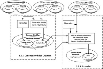
‘Raven’ is compared with each of the generic versions of the prototypes (tree, crow, city) using the Wu-Palmer similarity measure (Wu & Palmer, Reference Wu and Palmer1994) as implemented in NLTK version (Bird & Loper, Reference Bird and Loper2004) of WordNet (Fellbaum, Reference Fellbaum1998). The prototypes identified to be most similar are selected as the specific source prototype (‘large crow’) and the general source prototype (‘crow’). The general target prototype is the noun prototype (‘raven’) that is to be combined with the concept modifier (discussed in Section 3.2.2) to create the specific target prototype (‘large raven’). The interaction of these concepts is illustrated in Figure 4.
Graphical representation of the conceptual combination process for an adjective and a noun

The process of finding an appropriate sense of a preposition is slightly different. In the first step, all of the prototypes of the preposition in memory are returned as a list. The similarity measure used is the product of the Wu-Palmer similarity between the left nouns and the Wu-Palmer similarity of the right nouns. The adapted similarity measure allows Visuo to recognize that a ‘bird over forest’ is more similar to ‘bat over tree’ than it is to ‘clouds over forest’, even though the former shares a word in common (forest) and the latter does not. In this example, product similarity is calculated by the result of the bat's similarity to bird, multiplied by the result of forest's similarity to tree.
3.2.2 Concept modifier creation
Theory. We can imagine that an adjective modifies a noun (or noun phrase) in the mind of a reasoner. For example, we have an idea of what a dog looks like, and when specified that the dog is ‘small’, it changes the concept we have in mind. We view adjectives as functional entities that modify their associated noun phrases. This allows a reasoner to use adjectives to describe new concepts as long as the meaning of the adjective can be abstracted and transferred from a similar situation. We hold that reasoners have concept modifiers, which are created from adjective senses and used to modify nouns, creating new adjective–noun concepts. It is the instantiation of the functional capabilities of an adjective in a particular context. For example, a concept modifier created from the adjective ‘large’ as it is used for ‘crow’ can be applied to ‘raven’ to create a concept for ‘large raven’.
Implementation. Concept modifiers are implemented in Visuo as data structures that are comprised of one or more attribute modifiers. Attribute modifiers are data structures that represent how each attribute in a noun prototype is modified by an adjective prototype such that the noun prototype becomes an adjective–noun prototype. For example, if the prototype of a raven has two attributes, size and colour_brightness, and Visuo is performing conceptual combination on ‘large’ and ‘raven’, then up to two attribute modifiers will be created. More specifically, there is one attribute modifier for each attribute that is present in the general source, specific source, and general target prototypes. In the example shown in Figure 4, there is only one attribute modifier, since the only attribute present in all three concepts is Attribute B.
Attribute modifiers contain two distributions, a modifier density and a multiplier. The modifier density distribution is a normalized copy of the attribute's distribution of the general source prototype (e.g. ‘raven’). The multiplier is created by a piece-wise multiplication of the general source prototype by the specific source prototype. More formally, the multiplier m is a vector where each element is defined as
 $$m\, = \,\left( {\frac{{{{G}_{\rm{0}}}}}{{{{S}_{\rm{0}}}}},\,\frac{{{{G}_{\rm{1}}}}}{{{{S}_{\rm{1}}}}},\,\frac{{{{G}_{\rm{2}}}}}{{{{S}_{\rm{2}}}}},\, \ldots, \,\frac{{{{G}_{k\,{\rm{ - }}\,{\rm{1}}}}}}{{{{S}_{k\,{\rm{ - }}\,{\rm{1}}}}}}} \right)$$
where k is the size of the distributions, Gi is the ith element in the general source concept distribution, and Si is the ith element in the specific source concept.
3.2 Transfer
Theory. This section describes the creation of the novel concept (specific target concept), and how attributes are determined for it. In our running example, since crows are smaller than ravens, simply applying the concept modifier by multiplying the attribute modifiers’ multiplier distribution by the ‘raven’ attribute distributions would result in an inappropriate matching of the numbers in the distribution. In fact, without adjusting the distributions, a ‘large raven’ could have the distribution of what a ‘small raven’ should have, or it could have a distribution consisting of all zeros. So we conjecture that reasoners associate the values of the two distributions with the percent of the distributions that those values cover.
Implementation. Visuo creates a density distribution for the modifier values and one for the target prototype, which is a representation of how dense the data is at different parts of the distribution. For example, a density distribution might tell us that most of the data is in the low ranges, with very little in the high ranges. To make this, Visuo copies and normalizes the distribution of the source object's attribute. Normalization is defined here as transforming a distribution such that the sum of the distribution's values equals one. This density distribution is stored with the respective attribute modifier as the modifier density distribution. At this point, the multiplier is ready to be combined with the target prototype ‘raven’. The target density distribution is created by normalizing the target distribution.
Each value in the target distribution is multiplied by some percentage of the numbers in the multiplier. This percentage is determined by matching elements of the target density distribution to sections of the multiplier density distribution. For example, the first number in the target distribution might be multiplied by the first two, or even the first 2.6 numbers in the multiplier. If this percentage matching is not done, then large portions of distributions end up being unjustifiably multiplied by zero. To be more specific, the new attributes are created by the density distribution product (DDP, this algorithm is detailed in Section 3.3).
The final step is to create is the root concept, which, in our example, consists of three concepts: ‘large raven’, ‘above’, and ‘tree’. All that is missing for the merger is the concept of ‘above’ as it applies to this context. This is found once again by the WordNet's implementation of Wu-Palmer similarity measure, as described in the section on retrieval. The attribute values of ‘[[large bat] above [forest]]’ are used to create an exemplar and prototype of ‘above’ for the concept [[large raven] above [tree]]. The distribution is copied directly, rather than being created by changing a target with a multiplier, since there is no target to modify.
The creation of the complete novel concept is now complete.
3.3 DDP
The DDP is the result of multiplying two main distributions based on two density distributions. Each main distribution has an associated density distribution, which specifies the percent of coverage of each distribution, and is used to align the main distributions before the product is found. It allows the distributions to be molded onto each other before they are multiplied.
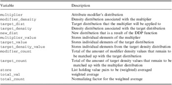
Detailed in this section is the pseudocode for the DDP algorithm as it applies to this model. Shown in Table 1 are descriptions of the variables used in the pseudocode. Following this, the algorithm is presented in pseudocode; the code is explained afterward.
Description of the variables in the pseudocode

3.2.1 Pseudocode algorithm
FUNCTION DDP (multiplier, modifier_density, target_dist, target_density):
modifier_count = 0
target_count = 0
new_dist = [ ]
multiplier_value = multiplier.next ()
modifier_count = modifier_density.next ()
FOR target_density_value in target_density:
store = [ ]
target_count = target_count + target_density_value
WHILE (target_count > modifier_count):
store.append ((modifier_count, multiplier_value))
target_count = target_count-modifier_count
IF multiplier.hasNext () AND
modifier_density.hasNext ():
multiplier_value = multiplier.next ()
modifier_count = modifier_density.next ()
END-IF
END-WHILE
IF (target_count < = modifier_count):
store.append ((target_count, multiplier_value))
modifier_count = modifier_count-target_count
target_count = 0.0
END-IF
total_count = 0
total_val = 0
FOR count, val in store:
total_count = total_count + count
total_val = total_val + count*val
END-FOR
IF total_count:
total_val = total_val/total_count
ELSE:
total_val = 0
END-IF
target_dist_value = target_dist.next ()
new_dist.append (total_val * target_dist_value)
END-FOR
RETURN new_dist
3.2.2 Pseudocode description
On line 1, the function takes in two distributions and two associated density distributions as described in Table 1. On line 5, new_dist is initialized as a new empty list. Lines 6 and 7 get the first values from the multiplier and the density distributions. The for-loop starting on line 9 iterates through each of the target_density values. Line 10 sets the store to a new empty list. Line 11 keeps track of the remaining amount of target_density values unaccounted for. The while-loop on line 13 checks for the case where there are more target_density values unaccounted for than modifier_density values. Line 14 adds a (weight, value) pair to the store, which will eventually be used in the weighted average. Line 15 removes the target_density values that have been accounted for. Line 17 checks if there are any multiplier and modifier_density values remaining, and if there are, gets them on the next two lines. Line 23 checks for the case where there are more modifier_density values unaccounted for then target_density values. Lines 29 to 41 calculate the weighted average of the value pair in store. On line 44, the weighted average is multiplied by the respective value in the target distribution. Lines 9 to 45 are repeated until all the new distribution values are calculated. Finally, line 47 returns the newly created distribution, which represents the newly adapted attribute distribution.
3.4 De-fuzzification
Once Visuo has a prototype that matches the input, the final step is de-fuzzification, which is the process of transforming a fuzzy qualitative distribution (such as an attribute's distribution) into a quantitative crisp number. The crisp number N is computed by taking a weighted average of the distribution as defined by:
 $$N\, = \,\frac{{{{\rSigma }_i}({{u}_i}\,\times \,{\rm{val(}}{{S}_i}{\rm{)}})}}{{{{\rSigma }_i}({{u}_i})}}$$
where, ui is the membership value in the distribution and val(Si) is the value of the fuzzy number (e.g. val(35F) = 35). The denominator Σi(ui) is used to normalize the result.
If we fuzzify the distribution of 175C, we get {0.0, 0.0, 0.0, 0.0, 0.0, 0.0, 0.0, 0.5, 0.9375, 0.5, 0.0625, 0.0, 0.0, 0.0, 0.0}. When this is de-fuzzified, output is the same as the original input: 175C.
3.5 Multiple attributes
As noted above, multiple attributes can be transferred for a single specific concept. For example, if one is asked to imagine a ‘large dog’, there is more to our imagined dog than simply a size. The dog has a color, a way it holds itself, and several other features. Up to this point, this paper has primarily only illustrated the generation of the estimate for a single attribute. Note, however, that Visuo will use the process described above for many attributes. Depending on the information in the memory, the imagined ‘large crow’ might come with quantitative estimates of wingspan, size, brightness, elevation, orientation, weight, etc., just as a person would.
To take a new example, suppose the target to be imagined is still ‘large raven’ but this time the reasoner retrieves and uses the ‘building’ prototype as its source, perhaps because there are few prototypes in memory. The conceptual combination only occurs for those attributes that the source and target prototypes share. The reasoner would not transfer the attribute ‘number-of-windows’ even though the building prototype has a distribution for it.
4 Evaluation
Evaluating Visuo. To evaluate the theory, we tested Visuo's implementation on input data collected from the online game Peekaboom (von Ahn et al., Reference von Ahn, Liu and Blum2006), which contains 57 797 images from the internet with labeled point clouds that identify the objects within it. For instance, an image containing a dog will have a set of points labeled ‘dog’. Roughly, these points show what part of the image should be associated with that label.
We used the spatial information of the objects in the Peekaboom database that were labeled as either cat, crow, dog, person, raven, skyscraper, and tower. The first 100 instances of each object were used, except for ravens and crows, since the database only contained 12 and 57 labels, respectively. Using the labeled points, the width-to-height ratio (which we will call the width ratio) of each object was used as input data for Visuo's Training Phase (Section 2.1). Width ratio rj for a particular object j is calculated by
 $${{r}_j}\, = \,100\,\times \,\left( {\frac{{\max ({{X}_j})\,{\rm{ - }}\,\min ({{X}_j})\, + \,15}}{{\max ({{Y}_j})\,{\rm{ - }}\,\min ({{Y}_j})\, + \,15}}} \right)$$
where Xj is the set of the x-components of all points labeled with object j, Yj is the set of the y-components of all points labeled with object j, max(Xj) and min(Xj) are the maximum and minimum values in Xj, and max(Yj) and min(Yj) are the maximum and minimum values in Yj.
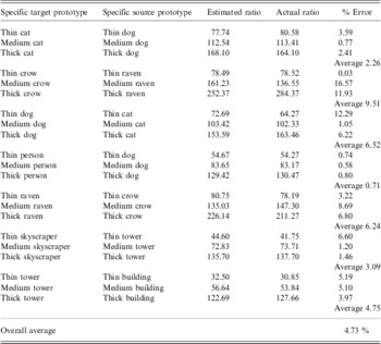
It is problematic to use only the width (or height) of the objects in the images since the concern is with the spatial properties of the object in the world frame as opposed to the image plane (i.e. we want a spatial attribute that represents the object and not just the picture of it). Any objective distance relation is unknowable without knowing the camera's distance from the object. Without knowing the intrinsic properties of the camera that took each image and the depth of all points in the image, it is impossible to infer (from the image alone) what the scale factor of the object in the image is. By using a ratio, we access the relation between distances, which is scale invariant (Table 2).
Comparison between Visuo's estimated width ratios and the actual width ratios

The Peekaboom data was collected with an online game in which two people who do not know each other are paired. One, the ‘boomer’, sees an image and an associated label. The other, the ‘peeker’, sees a blank screen. The boomer clicks parts of the image, which then get revealed to the peeker, who tries to type in the label the boomer is seeing. They receive points when the peeker guesses correctly.
When a boomer clicks a point on the image to reveal part of an object to his or her partner, all pixels within a 20 pixel radius are removed. Since this sometimes reveals pixels outside the image, we used an estimated value of 15, which we found to be a good compromise. For demonstration purposes, we multiplied each pixel count by 100 to translate it into mental units.
All training examples used from the database were labeled with either thin, medium, or thick (e.g. thick cat), except for the example containing the object to be visualized. For instance, if Visuo is asked to visualize [thick raven], then all examples aside from ravens would be labeled with the adjective. Of the labeled examples, the thinnest 30% are labeled as thin, the next 40% are labeled as medium, and the thickest 30% are labeled as medium. If the program works as our theory predicts, then it should guess that a thin raven's width ratio is more similar to crows than to the other concepts.
To evaluate the results, we used Visuo to visualize each specific target concept in Table 1. Visuo selected the specific source concept as a base for analogical transfer, and the estimated ratio was the ratio of the specific target concept as predicted by Visuo. The actual ratio is the ratio calculated directly from the database, and the error ε is calculated by
 $${\epsilon}\,{\rm{ = }}\,\left| {2\,\times \,\frac{{(\widehat{r}\,{\rm{ - }}\,r{\rm{)}}}}{{(\widehat{r}\,{\rm{ + }}\,r{\rm{)}}}}} \right|$$
where  $$\[--><$>\widehat{r}<$><!--$$
is the estimated ratio and r actual ratio.
As shown in Table 1, the results were very positive, with estimates very close to the actual values. The worst estimates were ‘medium crow’ (16.57%) and ‘thick crow’ (11.93%), which used ‘medium raven’ and ‘thick raven’ as a base, respectively. These estimates are quite reasonable considering the Peekaboom database only contained six instances of ‘medium ravens’ and three instances of ‘thin ravens’ to train from. Increasing the number of instances dramatically improves results, which can be seen with the width ratio prediction for a person. For all three person predictions, the error was 0.8% or less. Overall, the average error is 4.73%, indicating that the cognitive model Visuo can accurately estimate the quantities of unknown spatial attributes based on the quantities of semantically similar concepts.
Evaluating DDP. This portion of the evaluation consists of qualitative testing of Visuo's modification capabilities with primary emphasis on the DDP. We test the ability of the model to successfully alter the modification distribution to the context of the new targets. The figures in this subsection also give intuitions as to the inner workings of Visuo.
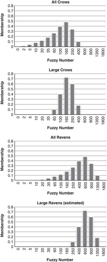
We ran three distribution tests: shifted, high variance, and low variance. In all tests, Visuo produced distributions that seemed reasonable and in line with expected performance. For the shifted distribution (e.g. large crows are smaller than large ravens), Visuo successfully shifted the distribution of large (see Figure 5). The ‘all crows’ distribution has the same shape, but is shifted to the left of the ‘all ravens’ distribution. The ‘large crows’ mean is around 160. If Visuo failed to shift the expected distribution of ‘large ravens’, the mean would be the same. As one can see from the ‘large ravens (estimated)’ distribution, representing what Visuo generates, you can see that the mean for the ‘large ravens’ is higher—over 600.
Visuo's performance when the target distribution is shifted from the source. The distribution for ‘all ravens’ is the same as that of ‘all crows’ except that it is shifted right. As expected, the distribution for ‘large ravens’ is shifted as well

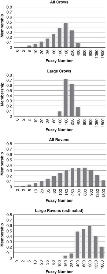
A high variance distribution occurs when there is large variance in the magnitudes of the spatial attributes. In the raven/crow example, if ravens have a greater range of sizes then the distribution would be flatterFootnote 3. If there is more variance in the size of ravens then there is in crows, then there should also be more variance in the size of large ravens than large crows (see Figure 6). Since the variance of the ‘large crows’ is small, Visuo would perform poorly if it predicted the range of ‘large ravens’ to be small as well, since ravens have a high variance. As you can see from the ‘large ravens (estimated)’ distribution in Figure 6, the estimated distribution shares the high variance of ‘ravens’.
Visuo's performance when the target has a higher variance. As expected, it adjusts the predicted distribution appropriately; the ‘large ravens’ distribution also has a high variance, even though the source distributions do not

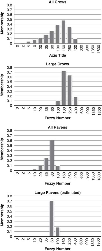
Finally, the results are similarly positive with the low variance condition (see Figure 7).
Visuo's performance in a low variance target situation. As expected, the estimated distribution also has a low variance

5 Conclusion
We have presented a computational theory of a part of visuospatial imagination: estimating quantitative values of spatial descriptors and relations given a qualitative input. This is an important cognitive task for counterfactual thinking, hypothetical thinking, planning, and simulation.
Our main claims are as follows. First, reasoners store quantitative perceptions as membership distributions across a logarithmic set of spatial magnitude detectors (analogous to fuzzy numbers). Second, these perceptions can be labeled with linguistic phrases. Third, when visualizing, reasoners will retrieve an appropriate prototype from memory, and determine the crisp output based on de-fuzzification of that magnitudes with a prototype. Fourth, when retrieval is impossible, reasoners analogically transfer and adapt meaning of these descriptors and relations from semantically related concepts.
In addition to the main claims, another contribution is the DDP algorithm. In this paper we have applied it to spatial relationships, but its application is potentially much broader. It is a very effective method for finding the product of two arbitrary distributions that do not match up well but need to be for a proper solution. Moreover, it allows distributions to be molded into a compatible distribution before a product is applied.
We have implemented this theory in a working Python computer program, and our preliminary results suggest that it behaves in a psychologically realistic way. Future work will compare the output of the program to participant data collected in psychological experiments.