In February of 1912, while addressing the Ohio Constitutional Convention, Theodore Roosevelt stated: “We hold it a prime duty of the people to free our government from the control of money in politics” (Reference Samuelson1912). Over a century later, the role of money in politics is no less important, nor less debated. According to the Center for Responsive Politics, in the last four decades the cost of electoral campaigns has grown significantly faster than inflation: in the 2012 electoral cycle, candidates spent $1.5 billion in Congressional races and $1.8 billion in the presidential race, over 60 percent more than eight years before.Footnote 1
In the 21st century, Roosevelt’s view that money in politics hampers accountability is still a widely held belief. According to recent polls, more than 75 percent of Americans support limits to electoral spending.Footnote 2 Several scholars (Jacobson 1980; Abramowitz 1991; Sorauf Reference Stewart1992; Gross, Goidel and Shields Reference Grossman and Helpman2002; Meirowitz Reference Monson and Curtis2008), however, have warned against the unintended consequences of existing regulatory solutions. Limiting the use of money in politics can have anti-competitive effects (Smith Reference Snyder and Strömberg1996; Sullivan Reference Wittman1998): by preventing candidates from publicizing their policy commitments, regulation can mute cash’s powerful megaphone (Cohen Reference Daley and Snowberg2012)—that is, money’s ability to disseminate valuable political information across the electorate.
This paper studies how the cost of political advertising, which we refer henceforth as “campaign cost” (ignoring other costly campaign activities such as get-out-the-vote), affects electoral accountability. Using a stylized model of electoral competition, we show that the effect of campaign cost depends critically on the level of partisan imbalance (defined as the ex ante competiveness of the electoral race). When partisan imbalance is low—that is, ex ante electoral competitiveness is high—an increase in the campaign cost always reduces politicians’ effort toward their constituents. In contrast, when partisan imbalance is high—that is, ex ante electoral competitiveness is low—an increase in the campaign cost can benefit voters. Greater campaign cost increases the incentives of the trailing candidate (i.e., the candidate who is electorally disadvantaged ex ante) to commit to a policy beneficial to voters. The trailing candidate is then more likely to win—this is the rebalancing effect—and voters more likely to obtain their preferred policy. We find empirical support for our core predictions when testing the model using data from the US House of Representatives.
Our theory of electoral accountability and campaign cost is predicated on two basic notions: (i) electoral communication has an informative role—that is, political advertising helps voters learn about candidates’ platforms—and (ii) in the absence of electoral incentives, voters’ and candidates’ objectives are not fully aligned. Building on a long tradition in formal theory, we study a parsimonious and tractable formal model satisfying those requirements.
The model features a representative voter, who is faced with the choice between two candidates running for a political office. Each candidate can commit to a low-effort policy or to a high-effort policy. The high-effort policy is a specific and verifiable activity that, relative to the low-effort policy, is beneficial for voters but costly for the politician (because it requires, e.g., mobilizing scarce resources like influence, time, and staff, or seeking expertise across traditional party lines). The low-effort policy can be interpreted as a commitment to the candidate’s party traditional platform, while the high-effort policy corresponds to a commitment to high level of constituency service.Footnote 3 Constituency service enhances a candidate’s electoral prospects, but requires communication through a costly advertising campaign, which we model as a discrete choice.Footnote 4 Unlike the cost of implementing the high-effort policy, which is paid only if a candidate is elected, the campaign cost is paid independently of the electoral outcome.
Our theoretical framework is best illustrated with an example. A congressional district is eligible for federal funds for repurposing an old industrial site and revamping its local economy. Candidates can either be vague about the issue and run a campaign focused on their party’s traditional platform (e.g., social justice or economic liberty), or tackle the issue by making specific, verifiable promises about exploiting the opportunity (e.g., obtaining permits or attracting public funds). The electoral success of the latter strategy crucially hinges on the candidate’s ability to spend time on the campaign trail and money on advertising to publicize his commitment. Its viability depends on the size of the costs associated with fulfilling such campaign promise once in office. How does a politician’s incentive to make these commitments depend on the campaign cost?
As voters get the benefit and none of the associated cost, they always would like candidates to commit to constituency service. In contrast, since commitment to the high-effort policy, in equilibrium, needs to be advertised, the presence of a positive campaign cost incurred regardless of the electoral outcome reduces candidates’ incentives to commit to voters’ preferred policy. As a consequence, voters are always better off when candidates could freely advertise their commitment. Furthermore, other things equal, a higher cost of advertising deepens the misalignment of interests between voters and politicians. Intuition thus suggests—against the idea of cash’s powerful megaphone—that there should always be a negative relationship between the campaign cost and electoral accountability, as measured by commitment to constituency service.
The main theoretical contribution of this paper is to show that the above intuition is correct only when the level of partisan imbalance is low. In that case, a higher campaign cost always reduces the likelihood that the high-effort policy is implemented. When, in contrast, imbalance is high, a greater campaign cost reduces the leading candidate’s incentive to commit to constituency service, as it becomes more costly to do so. As a result, the trailing candidate, who has little chance of winning the election if he chooses the low-effort policy, faces better electoral prospects when he promises a high level of constituency service. This increases his willingness to commit to the high-effort policy. Greater campaign cost then has a rebalancing effect: it improves the electoral chances of the trailing candidate.
Greater campaign cost can also improve electoral accountability. Voters benefit from the high-effort policy whenever at least one candidate commits to it. Therefore, the leading candidate’s commitment to constituency service matters only when the trailing candidate does not propose the high-effort policy. As the campaign cost increases, the trailing candidate is more likely to promise high effort, thereby limiting the impact of the leading candidate’s reduced commitment to constituency service. For high campaign cost, the increased probability of commitment by the trailing candidate dominates the reduced probability of commitment by the leading candidate, and voters are on average more likely to obtain their preferred policy.
The rebalancing effect of greater campaign cost has important implications for campaign finance regulation. Recent polls have shown that a majority of voters favors a publicly funded campaign finance system.Footnote 5 Our results, however, suggest that the electorate would not always benefit from subsidizing candidates’ campaign cost. When partisan imbalance and the campaign cost are low, candidates always propose high level of constituency service. Any public subsidy then can only reduce voter welfare: voters would bear part of the campaign cost without changing candidates’ behavior. When the campaign cost is high, a subsidy is very beneficial as it increases the likelihood one candidate commits to the high-effort policy. For intermediate levels of partisan imbalance and campaign cost, the effect is more subtle. Due to the rebalancing effect, when the campaign cost is relatively high, the trailing candidate is already very likely to promise constituency service so the cost of subsidizing campaigns tends to outweigh the benefit. When the campaign cost is relatively low, the leading candidate is likely to propose the high-effort policy, but the cost of incentivizing more effort is low so the benefit of a subsidy tends to outweigh its cost. Voters, however, may be better off taxing campaign expenditures to increase the campaign cost and benefit fully from the rebalancing effect at no cost.
Our theory generates novel and clear testable predictions regarding the relationship between politicians’ effort to secure benefits for their constituents, campaign cost, and partisan imbalance. Following established practices in the empirical literature on political accountability (Ansolabehere et al. 2003; Strömberg Reference Sulkin2004; Albouy Reference Albouy2009; Berry et al. Reference Bhattacharya2010; Snyder and Strömberg Reference Sorauf2010), we provide a first assessment of our theory using data from the US House of Representatives. In particular, we study the relationship between the per-unit price of political advertising (our proxy for the cost of informing voters) and district-level discretionary federal outlays (our proxy for constituency service) as a function of the difference in presidential candidates’ vote shares (our proxy for partisan imbalance). While federal outlays are an imperfect measure of a representative’s effort, the amount of resources expended by legislators to communicate such accomplishments to their constituents points to the importance of this type of activities (Druckman et al. Reference Egan2009; Grimmer et al. Reference Groseclose2012; Grimmer Reference Grimmer2013a; Grimmer 2013Reference Grimmer, Messing and Westwoodb).
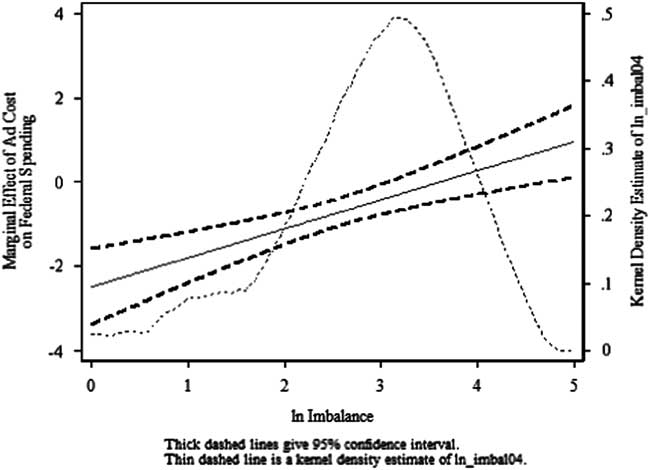
We find evidence in favor of our theory. When the level of partisan imbalance is low, more expensive political advertising is associated with lower federal discretionary spending. As partisan imbalance increases, however, the statistical association becomes weaker, and its sign eventually switches. In the top quartile of partisanship, an increase in the price of political advertising is associated with higher federal discretionary spending. This relationship is robust to the inclusion of key determinants of federal spending (e.g., seniority and committee assignment), as well as alternative specifications of the main variables of interest. We also provide suggestive evidence consistent with the proposed mechanism. Controlling for the level of imbalance, the marginal effect of greater campaign cost on constituency service is larger and more likely to be positive for “trailing” candidates (i.e., candidates from the relatively less popular party in the district) than for “leading” candidates (i.e., candidates from the relatively more popular party). These differences, however, are not statistically different at conventional level.
We conclude this introduction by connecting our work to the most closely related literature. A long tradition in formal theory studies how electoral incentives and partisan imbalance influence politicians’ behavior (Downs Reference Druckman, Kifer and Parkin1957; Wittman Reference Ansolabehere, Tripathi and Snyder1983; Calvert Reference Coate1985; Persson and Tabellini Reference Prat2000; Groseclose Reference Gross, Goidel and Shields2001; Aragonès and Palfrey Reference Ashworth2002; Ashworth and Bueno de Mesquita Reference Austen-Smith2006; Aragonès and Xefteris Reference Aragones and Palfrey2012). We depart from this literature by assuming that political communication is costly. Although we are not the first to introduce this assumption (Austen-Smith Reference Bailey1987; Grossman and Helpman Reference Hagen and Kolodny1996; Prat Reference Prato and Wolton2002; Bailey Reference Berry, Burden and Howell2004; Coate Reference Cohen2004; Ashworth Reference Ashworth and de Mesquita2006; Meirowitz Reference Monson and Curtis2008), there are important differences between the existing literature and this paper.
First, the cost of electoral campaigns is usually assumed to be borne by Special Interest Groups (SIGs) in exchange for political favors. Motivated by the idea that candidates, and not donors, choose the allocation of their electoral funds (and face the associated opportunity costs), and in light of the empirical evidence that direct campaign contributions per se do not affect policy stances (Ansolabehere et al. Reference Ansolabehere, de Figueiredo and Snyder2003), we assume that communicating with voters imposes a cost on candidates themselves.Footnote 6 In addition to its empirical foundations, this approach has substantive theoretical implications.Footnote 7
Second, the existing literature on costly campaigns focuses on adverse selection and/or ideological differentiation among candidates. In the present work we instead focus on constituency service, building on empirical evidence that the benefits received by districts (Druckman et al. Reference Egan2009) and politicians’ activism (Egan Reference Franz, Freedman, Goldstein and Ridout2014) play an important role in candidates’ communication strategies and electoral appeal. While we do not deny the importance of ideology in determining political outcomes, this paper shows how focusing on common value attributes leads to novel—and equally important—implications for campaign finance regulation.
The rest of the paper is organized as follows. First section describes our model of electoral accountability. Second section studies the effect of changes in campaign costs on the model’s key observables as well as on voter welfare. Third section discusses the model’s implication for campaign finance regulation. Fourth section presents a first empirical assessment of our theory’s key implications. Fifth section concludes.
A Model of Electoral Accountability
We consider a one-period model with two candidates and one representative voter (for which we reserve the pronoun “she”). Candidates (labeled L and R) compete for an elected office, which they value. Each candidate j∈{R, L} can either commit to a low-effort policy (p j =0), or to a high-effort policy (p j =1). Relative to a low-effort policy, the high-effort policy benefits the voter and entails an implementation cost (k>0) for the politician. This simple dichotomy captures the misalignment of incentives between politicians and voters when it comes to the provision of constituency service versus other activities (such as the pursuit of partisan goals, or undertakings associated with private returns for politicians). Electoral accountability in our setting is thus measured by commitment to the high-effort policy.
The voter learns a candidate’s policy platform (p j ) if and only if the candidate actively advertises it (y j =1, j∈{L, R}). While this assumption can be weakened (see Appendix B2), it allows us to focus on the informative role of political advertising in its starkest form. Communicating his platform (y j =1) is costly for a candidate (with symmetric cost c>0), as it requires time and effort on the campaign trail as well as spending on political advertising.
The voter’s payoff is normalized to 0 and 1 when the elected politician implements the low-effort and high-effort policy, respectively. The voter’s utility also depends on partisan shocks {ε
R
, ε
L
}, revealed to the voter before the election, but after candidates’ platform and communication choices. The partisan shocks capture the voter’s evaluation of candidates’ party label.Footnote
8
The shocks ε
j
are drawn from two (common knowledge) cumulative distribution functions with support
 $$\left[ {0,\,\bar{\epsilon }} \right],\,j\in \left\{ {L,\,\,R} \right\}$$
. Let
 $$ {\Pi}_{j} ={\rm Pr}(\epsilon _{j} \geq \epsilon _{{{\minus}j}} )$$
. Without loss of generality, we assume that П
R
∈ [1/2, 1).Footnote
9
The difference between Π
R
and Π
L
captures the level of partisan imbalance in favor of the right-wing candidate, to whom we then refer as the leading candidate (L is thus the trailing candidate). To simplify the derivation of the results, we also assume that the value of the partisan shocks cannot be too large:
 $\bar{\epsilon }\,\lt \,1$
. The voter’s utility, as a function of the elected candidate e ∈ {R, L}, is
 $$u_{v} (e)=p_{e} {\plus}\epsilon _{e} .$$
Candidates care about holding office.Footnote 10 If candidate j is elected and implements the low-effort policy, he enjoys a payoff normalized to 1. Such payoff is reduced by an amount k>0 if the elected politician chooses the high-effort policy p=1. We normalize the value of being out of office to 0. After choosing their platform, candidates choose whether to advertise it (at the incremental cost c>0) or not. Candidate j’s payoff is then given by
 $$u_{j} (p_{i} ,\,y_{i} )={\Bbb I}_{{\{ e=j\} }} (1{\minus}kp_{j} ){\minus}cy_{j} .$$
The policy cost k captures three possible aspects of an elected official’s job: (i) time and resources for constituency service (e.g., in the example developed in the introduction, time to secure subsidies, and attract private investors), (ii) the political capital required to build consensus and overcome veto players (Hall and Deardorff Reference Jacobson2006), and (iii) the opportunity cost of pursuing committee assignments linked to constituency interests (rather than their more suitable or desirable ones—for a ranking of committees, see Groseclose and Stewart Reference Strömberg1998; Stewart and Groseclose Reference Stewart and Groseclose1999; Stewart Reference Stewart and Groseclose2011).
The timing of the game is as follows:
1. Candidates choose a platform: low-effort (p j =0) or high-effort (p j =1) policy.
2. Candidates choose whether or not to advertise their platform: y j ∈ {0, 1}.
3. For each of the two candidates, the voter observes p j if and only if y j =1.
4. The voter observes the realization of the partisan shocks (ε L , ε R ).
5. The voter elects one of the two candidates, that is, e ∈ {L, R}.
6. The elected candidate implements p e , payoffs are realized.
In this model, candidates commit to the policy platform they choose.Footnote 11 We believe that, in this context, the commitment assumption can be justified on empirical grounds: campaign promises have strong predictive power on future behavior in the legislature (Sulkin Reference Sulkin and Swigger2009), especially on relatively more “common value” issues such as attracting new job-creating industries (Ringquist and Dasse Reference Roosevelt2004), even when these positions are implicitly embedded in highly symbolic campaign images (Sulkin and Swigger Reference Sullivan2008). A direct (and technically convenient) implication of this assumption is that communication can only affect a candidate’s chance of being elected. It does not change his payoff once elected.
Our equilibrium concept is perfect Bayesian equilibrium, with the additional restriction of excluding weakly dominated strategies. When multiple equilibria arise, we select the one associated with the highest payoff to the voter. In what follows, the term “equilibrium” refers to this class of equilibria.
Before proceeding to the analysis, we remark that due to the costs associated with the high-effort policy, a candidate commits to p=1 only if he has sufficient electoral incentives to do so. To make electoral accountability at least theoretically possible, we assume throughout that the implementing cost (k) and the campaign cost (c) are not too high compared with the benefit from office: c<1−k.
Campaign Costs and Electoral Accountability
We first study candidates’ advertising choice. Our model predicts a strong correlation between commitment to the high-effort policy and political advertising: a candidate pays the campaign cost if and only if he commits to p=1.Footnote 12 Candidates thus face a double cost of committing to the high-effort policy: the cost of implementing it (borne only if elected) and the cost of advertising this commitment to the voter (borne regardless of the electoral outcome).
LEMMA 1: A candidate j ∈ {L, R} pays the communication cost ( y j =1) if and only if he commits to the high-effort policy ( p j =1).
The intuition behind Lemma 1 is clear. A politician incurs the implementation cost k only if he commits to the high-effort policy. Hence, the low-effort policy can be understood as a candidate’s default option: he has no incentive to pay a cost to reveal that he proposes the low-effort policy. But this implies that, when choosing the high-effort policy, a candidate must advertise his platform.
A direct implication of Lemma 1 is that each candidate has effectively two feasible strategies: high-effort policy with a costly advertising campaign or low-effort policy without advertising campaign. When candidates commit to the same strategy, the voter’s electoral decision is driven by the partisan shocks (i.e., vote for R when ε R >ε L and vice versa—we can ignore draws which are 0 probability event). When candidates choose different policies, the voter always elects the candidate who proposes the high-effort policy due to our assumptions that the shocks are not too large. Table 1 represents the strategic interaction between the two candidates, and Proposition 1 describes the equilibrium of this electoral game.
The Electoral Game Induced by the Voter’s Behavior

PROPOSITION 1: Let
 $$k^{{\asterisk}} :=1{\minus}{{{\Pi}_{L} } \over {{\Pi}_{R} }}$$
. In equilibrium,
(i) If k≥k *, both candidates commit to the high-effort policy (p j =1, y j =1) if c≤(1−k)Π L , and to the low-effort policy (p j =0, y j =0) otherwise.
(ii) If k<k *, both candidates commit to the high-effort policy if c≤(1−k)Π L and choose the low-effort policy if c>Π R −k. When, instead, c ∈ ((1−k)Π L , Π R −k], candidate j commits to the high-effort policy with probability α j , where
 $$\alpha _{L} :={{k{\plus}c{\minus}{\Pi}_{L} } \over {{\Pi}_{R} {\minus}{\Pi}_{L} (1{\minus}k)}};\quad \alpha _{R} :={{1{\minus}k{\minus}c{\minus}{\Pi}_{L} } \over {(1{\minus}k){\Pi}_{R} {\minus}{\Pi}_{L} }}.$$
As pointed out above, a candidate commits to the high-effort policy if and only if the electoral reward is greater than the combined implementation (k) and campaign (c) costs. When these costs are very small, committing to the high-effort policy is a strictly dominant strategy for both candidates. Conversely, when these costs are very large, committing to the high-effort policy is a strictly dominated strategy for both candidates. The case of intermediate costs is more subtle. First, it is important to notice that the leading candidate R has an incentive to choose the same policy as L to take advantage of the favorable partisan shock. L, on the other hand, would prefer distinguishing himself from R (either to gain electorally or to avoid the costs of high effort with little electoral reward). This “hide-and-seek” game implies that the equilibrium can only be in mixed strategies.Footnote 13
The mixed strategy equilibrium can only arise when candidate R has a strong incentive to imitate L; that is, when partisan imbalance is sufficiently high. The range of the (c, k) space associated with a mixed strategy equilibrium thus depends on the degree of partisan imbalance: as Π R approaches 1/2, the support of the mixed strategy equilibrium converges to the empty set. Conversely, as Π R approaches 1, the area defined by c ∈ ((1−k)Π L , Π R −k] approaches the whole parameter space.
Having characterized the equilibrium, we now discuss how candidates’ behaviors are affected by the campaign cost c. When the equilibrium is in pure strategies, an increase in the campaign cost can only decrease candidates’ probability of committing to the high-effort policy. The reason is that the opportunity cost of committing to the high-effort policy increases, while the associated electoral reward remains unchanged. Consequently, voter welfare cannot be improved from c=0. When the equilibrium is in mixed strategies, the relationship between campaign cost and candidates’ incentives to commit to the high-effort policy depends on their ex ante electoral standing: the leading candidate R’s probability of commitment to high effort decreases with c, while it increases for the trailing candidate L.
COROLLARY 1:
(i) The voter welfare is maximized when c=0.
(ii) When the equilibrium is in mixed strategies, ∂α L /∂c>0 and ∂α R /∂c<0.
In a mixed strategy equilibrium (when imbalance is large enough), the two candidates’ decisions to commit to p=1 are affected by fundamentally different forces. The leading candidate R has an incentive to choose the high-effort policy only when the trailing candidate L chooses high effort with sufficiently large probability. In that case, choosing low effort is likely to result in a defeat, while matching the L’s platform allows him to exploit the favorable partisan shock. Conversely, the trailing candidate, who gains from distinguishing himself from the leading candidate, has a stronger incentive to choose high effort when his opponent chooses low effort with sufficiently large probability. As the campaign cost increases, equilibrium requires that the incentive to choose the high-effort policy increases for both candidates. For that to happen, it must be that the trailing candidate’ probability of choosing p=1 increases and that the leading candidate’s decreases. As a result, the overall probability that the trailing candidate wins the election increases with the campaign cost. This is the rebalancing effect.
What are the implications of the rebalancing effect for electoral accountability and voter welfare? When partisan imbalance is low, a greater campaign cost can only lower the probability that candidates commit to high effort and, therefore, can only reduce voter welfare. When partisan imbalance is large and the equilibrium is in mixed strategies, greater campaign cost affects L and R’s strategies in opposite directions, so the effect of higher c at first seems ambiguous. But it is important to notice that the voter benefits from the high-effort policy whenever at least one candidate commits to p=1. So R’s commitment to high effort matters only if the trailing candidate L does not promise the high-effort policy. For campaign cost close to (1−k)Π
L
, candidate L does not commit to p=1 with high probability so any reduction in R’s probability to commit to the high-effort policy decreases electoral accountability. For campaign cost close to Π
R
−k, candidate L commits to p=1 with high probability so a reduction in R’s probability to commit to the high-effort policy has little effect. As L’s probability to commit to p=1 increases with c, greater campaign cost improves electoral accountability for sufficiently large c (i.e.,
 $$c\in \left[ {{{1{\minus}k} \over 2},{\Pi}_{R} {\minus}k} \right)$$
).Footnote
14
Better electoral accountability then translates into higher voter welfare whenever the size of the partisan shocks is not too large.Footnote 15 This last condition ensures that the gain from obtaining the high-effort policy with greater probability dominates the loss in term of partisan shock from electing the trailing candidate L with higher probability.
PROPOSITION 2:
(i) An increase in the campaign cost strictly increases the probability that the high-effort policy is implemented if and only if c ∈ ((1−k)/2, Π R −k) and k<1−2Π L , and weakly decreases it otherwise.
(ii) There exists
 $$\hat{\epsilon }\,\gt\, 0$$
such that for all
$$\bar{\epsilon }\,\lt \,\hat{\epsilon }$$
, there exists
$$\underline {c}(\bar{\epsilon })\in ({{(1{\minus}k)} \mathord{\left/ {\vphantom {{(1{\minus}k)} {2,\,{\Pi}_{R} {\minus}k}}} \right. \kern-\nulldelimiterspace} {2,\,{\Pi}_{R} {\minus}k}})$$
such an increase in the campaign cost increases the voter welfare if and only if
$c\in (\underline {c}(\bar{\epsilon }),\,\Pi_{R} {\minus}k)$
and k<1−2Π
L
.


To summarize, our results show that an increase in the campaign cost (i) can only hurt the voter when partisan imbalance is low, but (ii) can also improve accountability when partisan imbalance is high, due to the rebalancing effect of higher c. To our knowledge, this result provides novel and qualified formalization of the notion of cash as a “powerful megaphone.” It is important to stress that these results do not rely on equilibrium selection: in the relevant range (c ∈ ((1−k)Π L , Π R −k]), the mixed strategy equilibrium that we consider is the unique equilibrium.
Implications for Campaign Finance Regulation
After having studied how exogenous changes in the campaign cost affect platforms and accountability, it seems natural to study the model’s implication for campaign finance regulation. Specifically, we characterize the optimal subsidy when, for a given c (determined by market forces in the media markets included in candidates’ district), the voter pays directly a portion s ∈ [0, c] of a candidate’s advertising cost, while leaving c−s to the candidate’s own fund-raising efforts.
To study the most favorable setting for campaign finance regulation, we assume that the subsidy enters linearly in the voter’s utility (i.e., there is no deadweight loss of taxation). Under this assumption, her objective function becomes p
e
+ε
e
−s(y
L
+y
R
). To simplify the analysis and focus on the effect of campaign cost, we also assume (without significant loss of generality) that (i) k is arbitrarily close to 0 and (ii) the partisan shocks are perfectly negatively correlated and have binary support
 $(\epsilon _{R} ,\epsilon _{L} )\in \left\{ {(\bar{\epsilon },0),(0,\,\bar{\epsilon })} \right\}$
.Footnote
16
The voter’s ex ante expected utility as a function of the subsidy s can be written as
 $$W(s)=\bar{\epsilon }{\plus}\alpha _{R} (1{\minus}\bar{\epsilon }{\Pi}_{L} ){\plus}\alpha _{L} (1{\minus}\bar{\epsilon }{\Pi}_{R} ){\minus}\alpha _{R} \alpha _{L} (1{\minus}\bar{\epsilon }){\minus}s(\alpha _{L} {\plus}\alpha _{R} ).$$
When c is already low enough so that both candidates already commit to high effort with probability 1 (in this simplified environment, when c<Π L ), any positive subsidy would simply transfer utility from the voter to the candidates without affecting their behavior. When, instead, the cost is large enough, the voter might gain from a positive subsidy. However, as Proposition 3 shows, the optimal subsidy (for the voter) is not always positive.
PROPOSITION 3:
Let
 $\tilde{c}={\Pi}_{R} {\minus}({\Pi}_{R} {\minus}{\Pi}_{L} )^{2} $
. The voter’s optimal campaign subsidy is
 $$s^{{\asterisk}} (c)=\left\{ {\matrix{ 0 \hfill & {c\leq \Pi _{L} } \hfill \cr {c{\minus}\Pi _{L} } \hfill & {c\in (\Pi _{L} ,\,\tilde{c}]} \hfill \cr 0 \hfill & {c\in (\tilde{c},\,\Pi _{R} ]} \hfill \cr {c{\minus}\Pi _{R} } \hfill & {c\in (\Pi _{R} ,\,1]} \hfill \cr } .} \right.$$
The voter obtains the high-effort policy whenever at least one candidate proposes it. As the voter must subsidize any candidate who engages in costly political advertising, when c>Π L , the best scenario for the voter is that one candidate commits to high effort with probability 1, whereas the other does so with probability 0.
This optimal scenario arises in two cases. First, when the campaign cost faced by candidates is Π R (i.e., c−s=Π R ), so that the rebalancing effect is strongest and the trailing candidate chooses high effort with probability 1. Second, when the campaign cost faced by candidates is Π L , so that the rebalancing effect is weakest and the leading candidate chooses high effort with probability 1. Whenever the initial campaign cost satisfies c>Π R , both c−Π L and c−Π R result in the same expected policy payoff, and the voter has a strict preference for the lowest of the two subsidies, c−Π R .Footnote 17
When the initial cost is below Π R , the rebalancing effect cannot be fully exploited. However, the trailing candidate L chooses the high-effort policy with high probability whenever c is close enough to Π R , while the subsidy c−Π L required to induce the advantaged candidate to choose high effort with probability 1 is very large. As a result, a campaign subsidy can only reduce voter welfare and the voter prefers 0 subsidy. When c is close to Π L , the gain from inducing greater effort by the leading candidate outweighs the cost, and the optimal subsidy is again positive.
Interestingly, our theory suggests that the voter would always prefer a tax on campaign spending rather than a subsidy for relatively large c. By raising the campaign cost by an amount Π R −c, the voter can take full advantage of the rebalancing effect (the probability of getting the high-effort policy increases) without using public resources. This negative subsidy is effectively a form of Pigouvian taxation: the voter would be better off even if she did not enjoy any direct benefit from the associated tax revenues.
Corollary 2: There exists c t ∈ (Π L , Π R ) such that for all c ∈ ( c t , Π R ), a tax t=Π R −c on campaign spending is optimal for the voter even if she does not enjoy the proceeds from it.
In our model, reducing the campaign cost improves the voter welfare because it increases the probability the voter’s preferred policy is implemented. As such, our theoretical framework develops an argument in favor of campaign finance even in the absence of SIGs exchanging contributions for political favors (as in Prat Reference Prato and Wolton2002; Coate Reference Cohen2004; Ashworth Reference Ashworth2005). To the best of our knowledge, the logic behind our results is novel. Our theoretical framework, however, also points out to the difficulty to design an optimal campaign finance reform: the welfare-maximizing subsidy (for the voter) depends critically on the current campaign cost and, under some condition, takes the form of a tax.
Testable Implications and Empirical Evidence
We now return to the positive implications of our model of electoral competition. Our theory predicts that the probability that the elected representative implements the high-effort policy should be as follows:
∙ negatively correlated with the campaign cost for low levels of partisan imbalance;
∙ positively correlated with the campaign cost for high levels of partisan imbalance;
∙ negatively correlated with the degree of partisan imbalance, holding constant the campaign cost.
In this section, we combine existing data sources from the US House of Representatives to present a prima facie cross-sectional empirical assessment of our theory. To perform this exercise, we need to find adequate empirical analogues for our three key variables: candidates’ effort, campaign cost, and partisan imbalance.
Drawing on a large body of research on the determinants of distributive politics in the United States (De Figueredo et al. 2003; Stromberg 2004; Albouy Reference Albouy2009; Berry et al. Reference Bhattacharya2010; Snyder and Strömberg Reference Sorauf2010), our proxy for a congressman’s effort is the amount of discretionary federal spending received by his home district (precisely, high variation non-defense federal outlays for the fiscal years 2006 and 2007).Footnote 18 It is indisputable that securing federal outlays captures only one dimension of electoral accountability. Furthermore, other political actors can influence the allocations of those funds (Berry et al. Reference Bhattacharya2010). Nonetheless, we believe that this approach has important advantages over alternative measures.
Theoretically, securing federal funds captures important aspects of our notion of high-effort policy. First, it is a relatively non-partisan activity for which the attribution of credit is simpler than other accomplishments (e.g., drafting legislation, or assembling a coalition supporting it), as witnessed by the fact that legislators from both parties heavily advertise these achievements (Druckman et al. Reference Egan2009; Grimmer et al. Reference Groseclose2012; Grimmer Reference Grimmer2013a; Grimmer 2013Reference Grimmer, Messing and Westwoodb). Second, there is robust evidence that voters tend to electorally reward these activities (Levitt and Snyder Reference McAfee and McMillan1997). Third, securing federal funds is a source of opportunity cost for politicians and is correlated with other forms of constituency service. Snyder and Strömberg (Reference Sorauf2010) document how representatives who are relatively more sheltered from electoral pressures due to exogenously low levels of media coverage are less likely to serve in committees representing their constituents’ interests, less likely to vote against their party, and less successful at securing federal funds (while they spend more time pursuing their broad political goals).
Empirically, federal outlays are easily measurable and display a large cross-sectional variance (a great virtue, given the limited availability of data on advertising cost). Moreover, as looking at federal outlays is a very common approach in the literature, our investigation can be guided by established practices and informed by clear benchmarks.
In line with existing literature, we measure partisan imbalance by the absolute distance in the vote share of the two presidential candidates in 2004.Footnote 19
For the campaign cost, we use data from the Wisconsin Advertising Project (Goldstein and Rivlin Reference Grimmer2007), which includes information on the number, length, and price of a large number of political TV ads aired during the 2004 congressional, gubernatorial, and presidential campaigns. Specifically, we approximate the campaign cost with the per-unit price of political advertising (30-second spot). It is important to point out that this variable captures only part of the cost of informing voters, which is determined by prices (taken as given) as well as quantities of ads necessary for a candidate’s message to reach the electorate (which depends on district characteristics). This is clearly a limitation of our empirical exercise.Footnote 20 However, we do not believe this limitation is too severe as (i) using per-unit average prices allows us to focus on an exogenous variable (not candidates’ strategic decisions), and (ii) total advertising expenditures are positively correlated with the per-unit cost of ads (see Evidence on the Mechanism section, where we also perform our analysis with total expenditures as a robustness check). Using per-unit price of ads also has some advantages. Indeed, we observe a candidate’s advertising expenditures only when he chooses to advertise. But our core comparative statics rely on all candidates, whether or not they advertise. With the per-unit price of ad, we approximate the campaign cost faced by candidates who chose not to advertise.
Due to data availability, our analysis is limited to the 109th Congress.Footnote 21 Drawing on our theory (and in line with the existing literature), we estimate the following model:
 $$y_{{is}} =\beta _{0} {\plus}\beta _{1} c_{{is}} {\plus}\beta _{3} \pi _{{is}} {\rm {\plus}}\delta \pi _{{is}} {\times}c_{{is}} {\plus}X_{{is}}^{'} \beta _{4} {\plus}\gamma _{s} {\plus}u_{i} .$$
Description of Variables

Note: ACS=American Community Survey.
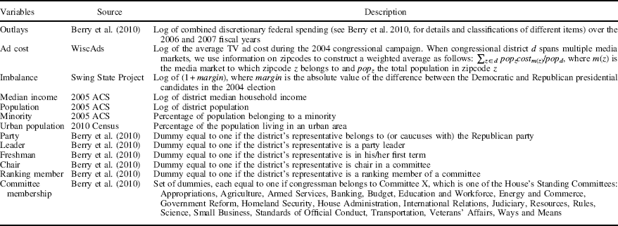
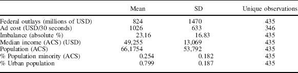
In our baseline specification, y is is the log of total federal outlays from “high variation programs” awarded to congressional district i in State s. This variable, described in detail in Berry et al. (Reference Bhattacharya2010), captures the amount of discretionary spending received by each district. c is measures the average price of a 30-second political ad for the 2004 electoral campaign in district i. It is constructed from a population-weighted average of the mean cost in each media market contained in district i. π is is the partisan imbalance in district i. X is is a vector of congressman-specific and district-specific controls: information on party, seniority status, membership and chairmanship of various committees, membership of party leadership from Berry et al. (Reference Bhattacharya2010), and on median income, population, shares of urban and minority population from the 2005 American Community Survey. γ s is a state fixed effects. Table 3 displays summary statistics for the main variables employed in our analysis. We restrict our baseline specification to the 295 congressional districts for which the available measure of ad cost covers at least 90 percent of the district population.
Summary Statistics

Note: ACS=American Community Survey.
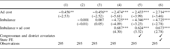
Table 4 reports the estimated coefficients from our baseline specification. Columns 1–4 show that partisan imbalance is not statistically associated with the level of federal outlays without the inclusion of the interaction term. Once the data are organized according to our theory, the coefficient of partisan imbalance and advertising cost are indeed negative and statistically significant, and the interaction term is positive and statistically significant (all three results are robust to the inclusion of district and congressman-specific covariates, as well as state fixed effects, as shown in columns 5 and 6).
Federal Outlays, Campaign Costs, and Partisan Imbalance

Note: Congressman and District covariates include median income, population, minority, urban population, party dummy, leadership dummy, freshman dummy, chair dummies, ranking dummies, and committee membership dummies. t-Statistics in parentheses (standard errors clustered at state level).
FE=fixed effects.
*, **, *** Significant at 10%, 5%, 1%, respectively.
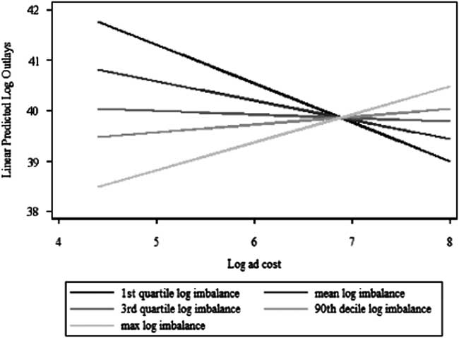
Figure 1 displays the marginal effect of ad cost on federal outlays (and its 95 percent confidence interval) implied by column (4) of Table 4. Consistent with our theory, the marginal effect is negative for low levels of partisanship and positive for high levels of partisanship, as illustrated by Figure 2, which displays the linear prediction of federal outlays as a function of ad cost for various percentiles of partisan imbalance.
Marginal effect of ad cost

Predicted value of federal outlays, by percentile of partisan imbalance

Evidence on the Mechanism
Our theory also has implications regarding the source of the joint effect of imbalance and campaign cost on accountability. In particular, under the assumptions of Proposition 2, an increase in the campaign cost should result in (i) higher constituency service (conditional on being elected) from the trailing candidate and (ii) lower constituency service (conditional on being elected) from the leading candidate.Footnote 22
To look for evidence of these differential effects, we create a dummy variable, Trailing, which equals 1 in districts where the representative comes from a different party than the presidential candidate who received the most votes in either of the two previous presidential elections.Footnote 23 Our theory predicts that
∙ the marginal effect of ad cost on constituency service should always be negative in the sub-sample of leading candidates (i.e., for all levels of imbalance);
∙ compared with the baseline estimates, the threshold level of imbalance above which the effect of ad cost is positive should be lower in the sub-sample of trailing candidates.
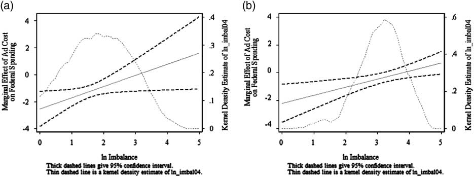
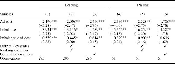
Figures 3(a) and 3(b) (as well as Table 5) show that the estimated marginal effects are larger for trailing than for leading candidates.Footnote 24 Specifically, in the sub-sample of trailing candidates, the (point estimate of the) marginal effect is positive for values of imbalance slightly above the median level in the overall population. In contrast, in the sub-sample of leading candidates, the (point estimate of the) marginal effect is positive only above the 88th percentile of imbalance.
Marginal effect of cost for (a) trailing candidates and (b) leading candidates

Separating Trailing and Leading Candidates

Note: District covariates include median income, population, minority, urban population. Ranking dummies include party dummy, leadership dummy, freshman dummy, chair dummies, ranking dummies. t-Statistics in parentheses (standard errors clustered at state level).
*, **, *** Significant at 10%, 5%, 1%, respectively.
It is important to stress that in a triple-interaction model, the estimated coefficient of Ad Cost×Imbalance×Trailing is positive, but not statistically different from 0 (see Table D1 in the Supplemental Appendix). Moreover, we cannot reject the hypothesis that the marginal effects of Ad Cost depicted in Figures 3(a) and 3(b) are equal across sub-samples.Footnote 25 While the lack of statistical significance can be due to the small sample size of the trailing sub-sample (only 51 observations), we can only claim that the evidence presented in this sub-section is on balance consistent with our theory, and only suggestive.
An Alternative Measure of Campaign Cost
In this sub-section, we consider total advertising expenditures as our measure of campaign cost, taking advantage of the fact that the Wisconsin Advertising Project contains data on the number of ads bought by candidates (provided by the Campaign Media Analysis Group, henceforth CMAG). The data set, however, contains only 129 districts with a positive number of recorded ads. This is an issue if the lack of observation is due to non-random missing data. This concern is mitigated by Hagen and Kolodny (Reference Hall and Deardorff2008), who argue that the CMAG data are reliable when it comes to the presence of advertising by candidates (however, they also argue that it is quite unreliable when it comes to total TV expenditures).
Consequently, we can use the presence of advertising to test another core prediction of our theory: candidates who advertise more should also secure more federal outlays for their district (Lemma 1). We thus construct a dummy variable called ads_dummy which equals 1 when we observe a positive level of political advertising, and 0 otherwise. Table D2 in the Appendix shows that ads_dummy has a statistically significant and economically meaningful association with federal outlays: in races with positive spending, federal outlays are between 55 and 95 percentage points higher than in districts without positive observed levels of spending.Footnote 26
We can also use data on the number of ads to test whether the per-unit price of ads is positively correlated with total advertising expenditures. We find that it is indeed the case: the quantity of ads decreases with price, but the associated elasticity is below unity when controlling for the quantity of ads by the opposing candidate (evidence available upon request). Finally, we use price and quantity to approximate candidates’ total advertising spending by each winning candidate (recall that this estimate is quite imprecise) and replicate the baseline analysis of Table 4 (on the restricted sample with positive advertising). Despite some loss of statistical significance (the loss in power is also substantial: the sample size no longer allows us to use state fixed effects), total expenditure, imbalance, and their interaction display a correlation pattern with federal outlays that is similar to the one documented in our baseline specification (Table D3 in the Appendix).
Discussion and Robustness Checks
Measurement of the advertising cost
The measurement of the cost of 30-second spots, has limitations that are widely acknowledged, despite the debate around their severity (Prior Reference Ringquist and Dasse2001; Monson and Curtis Reference Persson and Tabellini2003; Franz et al. Reference Goldstein and Rivlin2007; Hagen and Kolodny Reference Hall and Deardorff2008). In particular, Hagen and Kolodny (Reference Hall and Deardorff2008) find that within Pennsylvania, the cost figures reported in the CMAG data are likely to be overestimated and, more generally, suffer from measurement error. This problem is particularly severe when estimating total expenditures for each candidate. Our specification, however, is based on the average ad cost and, as a consequence, should be less sensitive to this issue. We also try to address this problem using an alternative measure of ad costs based on a larger sample that includes local and presidential races (see Appendix C and Table D4). We acknowledge, however, that the measurement issue is a limitation of any empirical analysis of the effect of campaign costs using CMAG data. Unfortunately, there is no alternative data source for advertising cost for the time period we consider.
Endogeneity concerns
One might suspect that the price of ads paid by candidates is correlated with the closeness of a race, and the statistical association that we find purely reflects demand shifts that resulted in higher price. We do not believe that this is a serious concern, for four reasons. First, and most important, our variable is constructed as a population-weighted average of the average ad price in each media market included in the district. Due to the imperfect geographic overlap between media markets and congressional districts, there must be an implausibly large geographic clustering of competitive races for the above described problem to be a serious concern. Second, in our regressions we always condition on partisan imbalance. Third, by Federal Communications Commission's (FCC) regulation, the price of political advertising is the lowest unit rate, which depends on overall demand for advertising in the media market. Fourth, in Appendix D, we explicitly test whether the closeness of a race affects ad prices. We find that the predictive power of partisan imbalance on ad costs is not statistically significant at any conventional level (see Table D6). If, in light of this evidence, one concludes that ad cost, but not partisan imbalance, is an exogenous variable for the purpose of our study, then the interaction term between ad cost and partisan imbalance can also be shown to be exogenous under certain conditions.Footnote 27
Sample selection
Our analysis could be affected by sample selection, as our baseline specification covers only 68 percent of the congressional districts. In Appendix D, we adopt a more generous cut-off for missing data on political ads (75 percent of the population), which allows us to cover almost 82 percent of the districts. The estimates are robust and almost unchanged (Table D7).
Additional robustness tests
In Appendix D, we report the result of several additional robustness tests. Our estimates are fully robust to the use outlays from each of the two fiscal years separately, as well as the use of a larger set of district-specific covariates from the 2000 Census.Footnote 28 Moreover, when we employ an alternative definition of partisan imbalance based on the 2000 presidential vote share or include designated market areas fixed effects (an extreme test, given that there are over 200 media markets), the point estimates lose statistical significance at conventional levels, but are relatively unchanged in size. Our estimates are similarly robust to the exclusion of outliers with respect to partisan imbalance (Table D12).
To conclude, our analysis uncovers robust and previously undocumented empirical patterns and shows that our theory provides a novel way to organize existing data sources. It is important to stress, however, that our estimates should be seen as a first pass which, we hope, will spark a more systematic and extensive empirical assessment. A clear answer as to whether these newly discovered patterns can be interpreted causally is left for future research.
Conclusion
In this paper, we study a model of electoral accountability where acting in voters’ interests once in office and advertising policy commitments during the campaign are both costly for politicians. We study how campaign cost affects politicians’ incentives to provide constituency service.
Our theory shows that higher campaign cost reduces electoral accountability and voter welfare when partisan imbalance is low. In contrast, we find that voters can benefit from a higher campaign cost when the level of partisan imbalance is high. Greater campaign cost has a rebalancing effect, which can result in higher expected level of constituency service, to the benefit of the electorate. We provide a prima facie empirical assessment of our theory. Evidence from the US Congress are consistent with our predictions and show that the mechanism we uncover is deserving of further empirical investigation.
This paper rationalizes the idea of “cash’s powerful megaphone,” whose pro-competitive effect on electoral races can be muted by campaign regulation. Indeed, we uncover circumstances under which voter welfare can only decrease as a result of a partial or full public financing of campaigns. More generally, our theory highlights that federal regulation of electoral campaigns can have highly heterogeneous effect on candidates’ choices and, ultimately, electoral accountability. In particular, and given its importance in the US context, widespread gerrymandering might systematically change the welfare consequences of campaign regulation.