


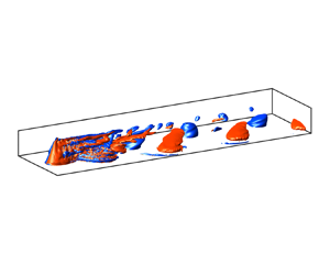





1. Introduction
The planet that we live on is full of multi-scale eddies, generated by various sources ranging from uneven thermal energy distribution at the largest scales, wind-driven ocean surface motions, to relatively more localised obstacle-induced flows. The dynamics of such eddies is greatly enriched by incorporating stratification, rotation and turbulence. Understanding this dynamics is essential to geophysics. This work will be focused particularly on the last example – wake eddies generated by obstacles.
In the deep ocean, seamounts and hills are stirring rods; they induce vortical motion, turbulence and internal gravity waves, which enhance heat and mass transport and hence crucially impact the ocean state. In the atmosphere, mountains commonly trigger wakes and waves, and orographic lifting is a source of convective weather, including air unsteadiness, formation of cumulonimbus clouds and precipitation. Both the ocean and the atmosphere are stratified, and the scales of motions are large enough to feel the effect of Earth's rotation, leading to a distinctive wake dynamics. The understanding of the wakes behind three-dimensional (3-D) obstacles from a fluid dynamics perspective would benefit the modelling and prediction of the multi-scale motions of oceanic and atmospheric bottom boundary flows.
In this study, we consider the wake of a steady uni-directional mean flow ( $U_\infty$) perturbed by an isolated conical seamount/hill submerged in the fluid (figure 1). The background has stable density stratification that is linear so that the buoyancy frequency
 $N=\sqrt {-g\partial _z \bar {\rho }/\rho _0}$ is a constant. Here,
 $\bar{\rho} + \rho_0$ is the unperturbed background density and
 $g$ is the gravitational acceleration. The Coriolis frequency
 $f_{c}=2\varOmega _{c}$ is a negative constant (Southern hemisphere). A conical obstacle of base diameter
 $D$ and height
 $h$ is placed on a flat bottom wall to represent an idealised isolated hill/seamount.
Flow configuration (not to scale). The background density is linearly stratified. The frame is rotating at a constant angular velocity  $\varOmega _{c}=\varOmega \sin \varphi$, where
 $\varOmega$ is the Earth's angular velocity and
 $\varphi$ is the latitude. The Coriolis frequency,
 $f_{c} = 2\varOmega _{c}$, is negative. Gravity, density stratification and the axis of rotation all point to negative
 $\hat{\boldsymbol{z}}$.

Two non-dimensional numbers, the vertical Froude number ( $Fr=U_{\infty }/N h$) and the Rossby number (
 $Ro=U_{\infty }/|\,f_{c}| D$) are the main controlling parameters. An additional (but not independent) non-dimensional number, the Burger number (
 $Bu=N^2h^2/f_{c}^2 D^2 =(Ro/Fr)^2$) that characterises the importance of stratification relative to rotation will also be used. The dynamical significance of the Burger number can also be interpreted as the normalised Rossby radius of deformation,
 $L_d/D=Nh/f_{c}D = \sqrt {Bu}$.
Stratified hill wakes have been studied extensively through laboratory experiments, field observations and numerical simulations. Hunt & Snyder (Reference Hunt and Snyder1980) showed experimentally that, for relatively strong stratification ( $Fr < 0.4$), there is a potential energy barrier below which the flow does not have sufficient kinetic energy to go over the hill and, instead, flows around the hill to form a quasi-two-dimensional (Q2-D) Kármán vortex shedding (VS) pattern. This is a significant qualitative difference between stratified and unstratified flow past a 3-D obstacle. Without stratification, the flow goes over the obstacle and horseshoe structures are formed (Garcia-Villalba et al. Reference Garcia-Villalba, Li, Rodi and Leschziner2009). Castro, Snyder & Marsh (Reference Castro, Snyder and Marsh1983) showed in stratified flow past a finite-span ridge that, as
 $Fr$ decreases from above to below unity, the wake behind the hill transitions from a lee-wave-dominated regime to a vortex-dominated regime, with the latter regime being the focus of this work. They found that at or below
 $Fr=0.2$ (their figure 7, last row), the modulation of the vortex wake by the lee waves can be neglected except near the peak of the ridge. Boyer et al. (Reference Boyer, Davies, Holland, Biolley and Honji1987) studied experimentally the effect of system rotation on stratified hill wakes in the regime of
 $Ro = O(0.1)$,
 $Fr = O(0.1)\unicode{x2013}O(1)$, equivalently
 $Bu = O(1)\unicode{x2013}O(10)$ variation. They found that the VS frequency is not strongly affected by changing
 $Ro$. However, the Reynolds number (
 $Re_D<1200$) was not sufficient for the wake to be turbulent. For non-rotating hill wakes, Vosper et al. (Reference Vosper, Castro, Snyder and Mobbs1999) varied the Froude number and the shape of the wake generator, and found that the VS frequency is a weak increasing function of
 $Fr$, and the
 $St$–
 $Fr$ relationships collapses for different object shapes if the reference velocity is corrected for blockage. More recently, Teinturier et al. (Reference Teinturier, Stegner, Didelle and Viboud2010) and Lazar et al. (Reference Lazar, Stegner, Caldeira, Dong, Didelle and Viboud2013a) performed laboratory experiments on the LEGI-Coriolis rotating platform where a cylinder (
 $h/D = 0.1$ was small) was towed in the upper layer of a fluid with two-layer stratification as a simple model of island wakes. The towing velocity and rotation speed were varied to achieve different combinations of
 $Ro$ and
 $Re$ with constant
 $Re/Ro$, e.g.
 $Ro =1$ corresponded to a Reynolds number of
 $Re = 10\,000$ in Teinturier et al. (Reference Teinturier, Stegner, Didelle and Viboud2010) and the experiments of Lazar et al. (Reference Lazar, Stegner, Caldeira, Dong, Didelle and Viboud2013a) considered
 $Re = 2000\unicode{x2013}7000$. With these laboratory experiments, they were able to investigate the asymmetry between cyclonic and anticyclonic vortices over a range of
 $Ro$.
For rotating stratified hill wakes, numerical studies include the utilisation of the hydrostatic regional oceanic modelling system (ROMS) (Shchepetkin & McWilliams Reference Shchepetkin and McWilliams2005), such as Dong, McWilliams & Shchepetkin (Reference Dong, McWilliams and Shchepetkin2007), Perfect, Kumar & Riley (Reference Perfect, Kumar and Riley2018), Perfect (Reference Perfect2019), Srinivasan, McWilliams & Jagannathan (Reference Srinivasan, McWilliams and Jagannathan2021) and Jagannathan et al. (Reference Jagannathan, Srinivasan, McWilliams, Molemaker and Stewart2021), and the hydrostatic version of the MIT general circulation model (MIT-GCM) (Marshall et al. Reference Marshall, Adcroft, Hill, Perelman and Heisey1997a,Reference Marshall, Hill, Perelman and Adcroftb), such as Liu & Chang (Reference Liu and Chang2018). Recently, Puthan, Sarkar & Pawlak (Reference Puthan, Sarkar and Pawlak2021) and Puthan, Pawlak & Sarkar (Reference Puthan, Pawlak and Sarkar2022a,Reference Puthan, Pawlak and Sarkarb) conducted non-hydrostatic large-eddy simulation (LES) of stratified hill wakes. The focus was on the role of tidal modulation of a mean current in a regime with strong stratification but weak rotational effects. The findings included tidal synchronisation (VS at specific tidal subharmonics that depend on the tidal excursion number), phases with enhanced turbulent dissipation and higher form drag. A similar numerical procedure will be followed in this work while excluding the periodic tide and focussing on rotation effects.
In terms of field observations, island wakes have acquired much attention recently and wakes have been studied near Palau (MacKinnon et al. Reference MacKinnon, Alford, Voet, Zeiden, Shaun Johnston, Siegelman, Merrifield and Merrifield2019; Zeiden et al. Reference Zeiden, MacKinnon, Alford, Rudnick, Voet and Wijesekera2021), the Green Island off the coast of Taiwan (Chang et al. Reference Chang, Jan, Liu, Cheng and Mensah2019) and in the lee of Guadalupe (Horvath et al. Reference Horvath, Bresky, Daniels, Vogelzang, Stoffelen, Carr, Wu, Seethala, Günther and Buehler2020), to name a few. A strong sign of a narrowband VS mode stood out from the broadband turbulence signal, and coherent submesoscale vortices were found in the wake. Submesoscale vortices are characterised by a Rossby number of order unity, and are receiving increasing attention (Taylor & Thompson Reference Taylor and Thompson2023).
In this paper, we present results from seamount/hill wakes at  $Fr = 0.15$ and three representative Rossby numbers,
 $Ro=0.15, 0.75, \infty$, corresponding to mesoscale, submesoscale and non-rotating stratified flow regimes, respectively. The conical hill has
 $h/D = 0.3$ and the Reynolds number is
 $Re = 10\,000$. There is near-wake turbulence but the focus of this paper will be on characterising coherent wake vortices that emerge further downstream.
The preceding literature survey raises several scientific issues regarding wakes of isolated topography in a rotating, stratified fluid. Previous simulations of an obstacle wake with significant stratification and rotation effects have used the hydrostatic assumption. In contrast, our non-hydrostatic model and LES approach (with high resolution as will be described) enables the capture of 3-D turbulent motions and, additionally, topographic internal gravity waves. The temporal frequency of VS from a conical obstacle in stratified flow can depend on the height of measurement at the obstacle in addition to background stratification and rotation. Current understanding of the VS frequency at a conical obstacle, which is based on a laboratory study (Boyer et al. Reference Boyer, Davies, Holland, Biolley and Honji1987) and hydrostatic simulations (Perfect et al. Reference Perfect, Kumar and Riley2018), as well as the spatial structure of the wake vortices, is incomplete. With the application of spectral proper orthogonal decomposition (§ 3) to vertical vorticity, we are able to not only pinpoint the VS frequency and its dependence on  $Ro$ (
 $Bu$) but also the spatial organisation of the associated coherent structure. Another question is the relation with linear stability theory of the stable coherent wake eddies (their vorticity and radius) that emerge in the simulations from the strongly turbulent near wake. A novel eddy identification scheme allows statistical measurement, based on a large ensemble of individual realisations, of the wake-eddy structure and its evolution as a function of downstream distance (§ 4). Our comparison with stability theory (§ 5) expands on the important laboratory findings of Lazar et al. (Reference Lazar, Stegner, Caldeira, Dong, Didelle and Viboud2013a) in various ways: substantially higher
 $Re = 10\,000$ at
 $Ro = 0.15$ relative to the laboratory value of
 $Re = 1500$, the non-uniform cross-section of a cone instead of a cylinder and a continuous linear stratification instead of a two-layer stratification.
The rest of the paper is structured as follows: § 2 introduces the numerical methods and the LES simulations conducted as part of this work; § 3 elucidates the global structures in the flow that are coherent in space and time via flow visualisations and spectral proper orthogonal decomposition (SPOD); § 4 presents ensemble-averaged tracks of the centres of vortices that are obtained by application of a pattern recognition method; § 5 is a systematic study of the asymmetry between cyclones and anticyclones and the instabilities of the anticyclones; § 6 concerns the evolution of the mean momentum wake; and, finally, § 7 is a summary and discussion of the results.
2. Numerical simulations
The incompressible Navier–Stokes equations are solved in a Cartesian coordinate system with  $x,y$ and
 $z$ being the streamwise, transverse and vertical directions, as shown in figure 1. In the momentum equation, density variation appears only in the buoyancy as per the Boussinesq approximation and system rotation is represented by the Coriolis force. The non-dimensional governing equations in index notation are as follows:
 $$\begin{gather} \frac{\partial u_i}{\partial x_i} = 0, \end{gather}$$
 $$\begin{gather}\frac{\partial u_i}{\partial t} + \frac{\partial u_i u_j}{\partial x_j} - \frac{1}{Ro} \epsilon_{ij3} (u_j - U_{\infty}\delta_{j1}) ={-} \frac{\partial p^*}{\partial x_i} + \frac{\partial \tau_{ij}}{\partial x_j}- \frac{1}{Fr_D^2} \rho^*\delta_{i3}, \end{gather}$$
 $$\begin{gather}\frac{\partial \rho}{\partial t}+ \frac{\partial \rho u_i}{\partial x_i} = \frac{\partial {{J}_{\rho,i}}}{\partial x_i}, \end{gather}$$
 $$\begin{gather}\tau_{ij} = \frac{1}{Re} \left(1 + \frac{\nu_{sgs}}{\nu} \right) \left(\frac{\partial u_j}{\partial x_i} + \frac{\partial u_i}{\partial x_j}\right),\quad {J_{\rho,i}} = \frac{1}{RePr} \left(1 + \frac{\kappa_{sgs}}{\kappa} \right)\frac{\partial \rho}{\partial x_i}, \end{gather}$$
where the normalising units for  $x_i$,
 $u_i$,
 $t$,
 $p^*$ and
 $\rho ^*$ are
 $D$,
 $U_{\infty }$,
 $D/U_{\infty }$,
 $\rho _0 U_{\infty }^2$ and
 $-\partial _z \bar {\rho } D$, respectively. In the above equations,
 $\delta_{ij}$ is the Kronecker Delta,
 $\epsilon_{ijk}$ is the Levi-Civita symbol and
 $\tau_{ij}$ is the deviatoric stress tensor. Here, the horizontal Froude number,
 $Fr_D=U_{\infty }/ND$, is related to the vertical Froude number used in this study as
 $Fr_D = (h/D) U_{\infty }/Nh = (h/D) Fr = 0.045$. The Prandtl number,
 $Pr=\nu /\kappa$, which is the ratio between the molecular viscosity
 $\nu$ and the scalar diffusivity
 $\kappa$, is set to unity.
The total density  $\rho$ is decomposed into the reference density
 $\rho _0$, the linearly varying background density
 $\bar {\rho } (z)$ and the density perturbation
 $\rho ^*$ due to fluid motion
 \begin{equation} \rho(x,y,z,t) = \rho_0 + \bar{\rho}(z) + \rho^*(x,y,z,t). \end{equation}
The total pressure is written as
 \begin{equation} p(x,y,z,t) = p_0 + p_g(y) + p_a(z) + p^*(x,y,z,t), \end{equation}
where the reference pressure  $p_0$ is a constant, the hydrostatic (ambient) pressure
 $p_a$ has a vertical gradient that balances the ambient density (
 $\rho _a=\rho _0 + \bar {\rho }(z)$) and the geostrophic pressure
 $p_g$ has a transverse gradient that balances the Coriolis force due to the velocity
 $U_{\infty }$ of the free stream. Only the dynamic pressure
 $p^*$ appears in the momentum equation (2.2).
The LES is performed at a moderately high Reynolds number  $Re_D = U_{\infty } D/\nu = 10\,000$. Spatial derivatives are discretised with a second-order central finite difference on a staggered grid, and the equations are advanced in time using a combined scheme with third-order Runge–Kutta for the convection terms and Crank–Nicolson for the diffusion terms. Continuity is enforced by solving the pressure Poisson equation. The obstacle is represented by an immersed boundary method (Balaras Reference Balaras2004; Yang & Balaras Reference Yang and Balaras2006). The sub-grid-scale (SGS) model is chosen to be the wall-adapted local eddy-viscosity (WALE) model (Nicoud & Ducros Reference Nicoud and Ducros1999) with the SGS Prandtl number
 $Pr_{sgs}=\nu _{sgs}/\kappa _{sgs}$ set to unity, where the SGS viscosity
 $\nu _{sgs}$ and diffusivity
 $\kappa _{sgs}$ represent the modelled effects on the transport of resolved momentum and scalar by the unresolved scales. For more numerical details, the reader is referred to Puthan et al. (Reference Puthan, Jalali, Ortiz-Tarin, Chongsiripinyo, Pawlak and Sarkar2020).
The conical obstacle has base diameter  $D$, height
 $h$ and a slope of approximately
 $30^\circ$ (
 $28.4^\circ$) such that
 $h/D = 0.3$. The slope of approximately
 $30^\circ$ in this study is steep in the oceanic context, both dynamically (much larger than typical internal wave propagation angles) and geometrically (typically, underwater bathymetry has much smaller slope angle).
The computational domain spans a volume of  $L_x \times L_y \times L_z = [-4,15] \times [-4,4]\times [0, {4}]$ in units of
 $D$ and the horizontal resolution of the immersed body and the turbulent near wake (
 $-1< x/D<2$) is held constant at
 $(\Delta x, \Delta y)\approxeq (0.003D,0.006D)\le (4\eta, 8 \eta )$, with a mild stretching in the streamwise direction. Here,
 $\eta$ is the minimum Kolmogorov length scale at the centreline at different heights. The vertical resolution below
 $z/h=1.2$ is kept at
 $\Delta z = 0.008h \approxeq 0.05 U_{\infty }/N$ to resolve the length scale for vertical overturning motion
 $U_{\infty }/N$.
The inflow condition is a uniform velocity inlet, and the outflow is a Neumann-type convective outlet. The lateral boundaries are periodic to reduce the blockage effect and to allow the wake to flap. The top boundary is shear free, and the hill boundary is no slip for velocity and no flux for density. Sponge layers are placed at the inlet and the top boundaries to reduce spurious reflected internal wakes. The overall LES setting and the immersed boundary formulation have been tested and validated against available data on force coefficients and evolution of wake deficit and turbulence intensity for flow past various geometries (sphere, disk, cone) in unstratified and stratified environments (Pal et al. Reference Pal, Sarkar, Posa and Balaras2016, Reference Pal, Sarkar, Posa and Balaras2017; Chongsiripinyo & Sarkar Reference Chongsiripinyo and Sarkar2020; Puthan et al. Reference Puthan, Jalali, Ortiz-Tarin, Chongsiripinyo, Pawlak and Sarkar2020).
The parameter space explored is shown in table 1. The stratification is held constant at  $Fr = 0.15$, a typical value for midsize topography in the ocean and the atmosphere, and is in the ‘flow-around’ regime where coherent wake vortices dominate. Meanwhile, the rotation Rossby number is varied as
 $Ro=0.15, 0.75, \infty$, to study its effect on the vortex wake. These three values of
 $Ro$ correspond to mesoscale, submesoscale and non-rotating geophysical flows. The induced Burger numbers are
 $Bu = 1, 25, \infty$, which will be used to label different cases.
Parameters of simulated cases. Here,  $N_x,N_y,$ and
 $N_z$ are the number of grid points in each direction and
 $N_t$ is the total number of available snapshots that will be used for all statistics. Also,
 $T$ is the time span of the stored data. The aspect ratio of the conical obstacle is
 $h/D = 0.3$ for all cases.

We compile a time-resolved numerical database that consists of three rotation strengths and collect the data after statistical stationarity is reached. Each case has  $N_t=4000$ snapshots that span around 300 convective time units (
 $T = 300 D/U_{\infty }$), which corresponds to roughly
 $80$ VS periods. Statistics, to be discussed later, are obtained by averaging over the entire interval,
 $T$.
3. Large-scale coherent structures
In geophysical flows, coherent vortical structures are commonly observed. There is no universal definition of coherent structures, but they are generally strong enough and have a relatively independent dynamics to distinguish them from the background flow, account for a significant portion of the fluctuation energy of the system, are spatially organised and their lifetime is sufficient for them to be dynamically important. The wake eddies of this paper have the aforementioned features.
Large-scale Kármán vortices, a specific type of coherent structure, are associated with VS from bluff bodies. In geophysical applications, they are commonly found in flows impinging on bottom or side topography, e.g. island wakes (Young & Zawislak Reference Young and Zawislak2006; Chang et al. Reference Chang, Jan, Liu, Cheng and Mensah2019; Horvath et al. Reference Horvath, Bresky, Daniels, Vogelzang, Stoffelen, Carr, Wu, Seethala, Günther and Buehler2020), headland wakes (Pawlak et al. Reference Pawlak, MacCready, Edwards and McCabe2003) and in laboratory flows (Hunt & Snyder Reference Hunt and Snyder1980; Castro et al. Reference Castro, Snyder and Marsh1983; Boyer et al. Reference Boyer, Davies, Holland, Biolley and Honji1987; Teinturier et al. Reference Teinturier, Stegner, Didelle and Viboud2010), among others. In field observations and laboratory experiments, the features of the coherent vortices are inferred from single- or multiple-point statistics and flow visualisations. The data are limited in spatial coverage and resolution.
In what follows, coherent structures will be studied in two ways. First, individual snapshots in which vortex structures are vividly visible are used for a qualitative overview of rotation effects (§ 3.1). Second, a more comprehensive quantitative assessment is obtained by applying SPOD to the time-resolved LES database in table 1 to reveal the statistical significance of the coherent structures. Section 3.2 reviews the theory and implementation of SPOD, followed by the analysis of the temporal eigenspectra (§ 3.3) and spatial modes (§ 3.4).
3.1. Flow visualisations
A first impression of the 3-D spatial organisation of the wake vortices is provided by the isosurfaces of the vertical component of vorticity ( $\omega _z=(\boldsymbol {\nabla } \times \boldsymbol {u})_z$) in figure 2(a–c) for cases BuInf, Bu25 and Bu1, respectively. At moderately strong stratification (
 $Fr\le O(0.1)$), vertical overturning motions are suppressed to approximately one order of magnitude smaller than horizontal flows, with the latter well represented by
 $\omega _z$.
Visualisation of the isosurfaces of  $| \omega _z | D/U_{\infty }=1.5, 1.0, 3.0$ for BuInf, Bu25 and Bu1 (top to bottom), respectively. Red and blue indicate positive (anticyclonic since
 $f_{c}$ is negative) and negative (cyclonic) vorticity, respectively. Note the vertical axis is normalised with the height
 $h$ of the hill, which is approximately
 $0.3$ times the base diameter
 $D$. The three snapshots (a–c) are taken at time instants
 $tU_{\infty }/D=252.0, 221.6, 152.0$, respectively.

In the near-wake region ( $x/D<3$), the
 $\omega _z$ isosurface is space filling and multiscale, indicating greater turbulence intensity than further downstream. But after
 $x/D=3$, the vortices quickly organise into spatially compact coherent structures that persist to the end of the computational domain with little change. Rotation clearly influences the shape and size of the structures. For case BuInf in figure 2(a), the structures are slanted ‘tongues’ with horizontal dimensions greater than their height. As the strength of rotation is increased, the horizontal size shrinks and the height increases as in figure 2(b) for Bu25. With further increase of rotation, the vortex structures become aligned with the vertical axis, appearing as tall ‘columns’ that extend from the flat bottom to the hill height, in figure 2(c).
The wake vortices are composed of cyclones (rotation is in the same direction as that of the frame) and anticyclones. It is found in figure 2(b,c) that, with the presence of rotation, the cyclones (negative vortices in blue) are different from anticyclones (positive vortices in red) with regards to size, shape and vorticity distribution, as will be elaborated in later sections. In figure 2(c), cyclones are taller and thinner than anticyclones and, as will be shown, have stronger interior vorticity.
Figure 3(a–c) shows the instantaneous  $\omega _z$ at several heights for all three cases. In all three cases, a pattern of Q2-D Kármán vortices is distinct in all planes at
 $z/h=0.12, 0.25, 0.75$. The flow is akin to a vortex wake rather than its unstratified counterpart of a 3-D turbulent wake (Garcia-Villalba et al. Reference Garcia-Villalba, Li, Rodi and Leschziner2009).
(a–c) Instantaneous and (d) time-averaged  $\omega _z$ at horizontal planes at
 $z/h=0.75, 0.50, 0.12$ (from top to bottom in each panel). (a,d) Cases BuInf, (b) Bu25, (c) Bu1. In (a–c), the snapshots are taken at non-dimensional time instants
 $tU_{\infty }D= 77.9, 123.9,63.3$ counted after the fully developed state is reached, respectively.

The mean vertical vorticity ( $\langle \omega _z \rangle$) of case BuInf is shown in figure 3(d). For the lower two planes, the mean looks very similar to those obtained in low Reynolds number 2-D cylinder wakes, such as in Barkley (Reference Barkley2006) and Mittal (Reference Mittal2008), both at
 $Re_D=100$. Such similarity supports the Q2-D feature of the hill wake at
 $Fr=0.15$. At the same time, there is a notable difference: the flow in each horizontal place that cuts the hill does not represent an independent 2-D flow around a cylinder with the local hill diameter. Among different planes at different heights in figure 3(d), the length of the attached shear layer (with dark colours), is approximately a constant, regardless of the variation of the local hill diameter. This is consistent with the fact that the VS frequency is a global constant which will be discussed in detail in the next section, as the shear layer length is correlated to the shedding frequency (Williamson & Brown Reference Williamson and Brown1998).
In the SPOD analysis of the next section, the vertical vorticity on different horizontal planes ( $\omega _z(x,y,t;z)$) is chosen as the quantity of interest since the large-scale wake structures involve predominantly Q2-D vortical motion (figures 2–3), the shedding and evolution processes of which are well represented by
 $\omega _z$. Moreover, the focus of this work is on the influence of increasing rotation strength on the horizontal motions, which tends to constrain the flow to be around the vertical axis at the large scales and significantly enhances
 $\omega _z$, as will be shown later. In the rotating cases Bu25 and Bu1, the stability of the anticyclones will also be studied (§ 5) with
 $\omega _z$ being one of the most important metrics, hence we apply
 $\omega _z$ rather than other vortex identification criteria for overall consistency.
As seen in figures 2–3,  $\omega _z$ structures exhibit dissimilar vertical organisation at different levels of rotation, although Kármán vortices are present in each horizontal plane. Owing to stratification, a vertical length scale of
 $U_{\infty }/N = Frh = 0.15h$ is introduced to the flow, and whether vortex structures remain coherent over vertical distances larger than
 $U_{\infty }/N$ regardless of rotation (suggested affirmatively by figure 2) needs quantitative investigation. To that end, we perform SPOD on vertically offset horizontal planes at
 $z/h=0.12, 0.25,0.50,0.75$ (
 $N_x\times N_y\times N_z=1538\times 1280\times 1$) and the vertical centre plane at
 $y=0$ (
 $N_x\times N_y \times N_z=1538\times 1\times 320$) to allow the choice of different dominant (VS) frequencies at different heights by the flow and avoid imposing a priori a global frequency.
3.2. Spectral proper orthogonal decomposition and its numerical implementation
Proper orthogonal decomposition (POD) is a matrix-factorisation-based modal decomposition of complex systems introduced into fluid mechanics by Bakewell & Lumley (Reference Bakewell and Lumley1967) and Lumley (Reference Lumley1967, Reference Lumley1970).
Consider a statistically stationary square-integrable multi-variable signal  $\boldsymbol {q}(\boldsymbol {x},t) \in \mathcal {L}_{{{\boldsymbol{\mathsf{W}}}}}^2(\boldsymbol {\varOmega })$ with zero mean. Here,
 $\mathcal {L}^2_{{{\boldsymbol{\mathsf{W}}}}}$ is the Hilbert space equipped with a weighted inner product
 \begin{equation} (\boldsymbol{q}_1, \boldsymbol{q}_2)_{{{\boldsymbol{\mathsf{W}}}}} = \int_{\boldsymbol{\varOmega}} \boldsymbol{q}_2^{H}(\boldsymbol{x}) {{\boldsymbol{\mathsf{W}}}}(\boldsymbol{x}) \boldsymbol{q}_1(\boldsymbol{x})\,{\rm d}\kern0.07em\boldsymbol{x} ,\end{equation}
on a bounded domain  $\boldsymbol {\varOmega }$, and
 $({\cdot })^{H}$ denotes Hermitian transpose. The weight matrix
 ${{\boldsymbol{\mathsf{W}}}}$ is Hermitian positive–definite and the weighted
 $2$-norm is defined as
 $\|\boldsymbol {q}_1\|_{{{\boldsymbol{\mathsf{W}}}}}=(\boldsymbol {q}_1,\boldsymbol {q}_1)_{{{\boldsymbol{\mathsf{W}}}}}^{1/2}$. The symbol
 $\langle {\cdot } \rangle _{E}$ denotes the ensemble average over all realisations, and it is equivalent to the time average under ergodicity. The goal of POD is to find an empirical function
 $\boldsymbol {\psi }(\boldsymbol {x})$ that solves the optimisation problem
 \begin{equation} \boldsymbol{\psi}(\boldsymbol{x}) = \arg \max_{\|\boldsymbol{\psi}\|_{{{\boldsymbol{\mathsf{W}}}}}=1} \langle (\boldsymbol{q},\boldsymbol{\psi})_{{{\boldsymbol{\mathsf{W}}}}} \rangle_{E}, \end{equation}
which defines  $\boldsymbol {\psi }(\boldsymbol {x})$ as the function on which the projection of
 $\boldsymbol {q}(\boldsymbol {x},t)$ is maximised in the sense of the least squares. Since
 $\mathcal {L}^2_{{{\boldsymbol{\mathsf{W}}}}}$ is an infinite-dimensional space, a practical way to obtain the empirical function
 $\boldsymbol {\psi }(\boldsymbol {x})$ is to approximate it within a finite-dimensional space spanned by
 $\{\boldsymbol {\psi }^{(i)}\}_{i=1}^{M}$, where
 $\boldsymbol {\psi }^{(i)}$ is the
 $i$th spatial mode and
 $M$ is the order of truncation. It was shown in Holmes et al. (Reference Holmes, Lumley, Berkooz and Rowley2012) that the optimisation problem (3.2) can be converted to a Fredholm eigenvalue problem as
 \begin{equation} \mathcal{R} \boldsymbol{\psi}^{(i)}(\boldsymbol{x}) = \int_{\boldsymbol{\varOmega}} {{\boldsymbol{\mathsf{R}}}}(\boldsymbol{x},\boldsymbol{x}'){{\boldsymbol{\mathsf{W}}}}(\boldsymbol{x}') \boldsymbol{\psi}^{(i)}(\boldsymbol{x}')\,{\rm d}\kern0.07em\boldsymbol{x}' = \lambda^{(i)} \boldsymbol{\psi}^{(i)}(\boldsymbol{x}), \end{equation}
where  $\mathcal {R}$ is a linear operator and
 ${{\boldsymbol{\mathsf{R}}}}(\boldsymbol {x},\boldsymbol {x}')= \langle \boldsymbol {q}(\boldsymbol {x}) \boldsymbol {q}^{H}(\boldsymbol {x}') \rangle _{E}$ is the two-point correlation tensor. Since
 ${{\boldsymbol{\mathsf{R}}}}$ is Hermitian positive–definite, its eigenvalues
 $\lambda ^{(i)}$ are real positive that each represents a fraction of the fluctuation energy, and the eigenvectors
 $\{\boldsymbol {\psi }^{(i)}\}_{i=1}^{M}$ form an orthogonal basis under the inner product (3.1).
In the framework of SPOD, the eigenvalue problem (3.3) is cast as
 \begin{equation} \mathcal{R} \boldsymbol{\psi}^{(i)}(\boldsymbol{x},t) = \int_{\boldsymbol{\varOmega}} \int_{-\infty}^{\infty} {{\boldsymbol{\mathsf{R}}}}(\boldsymbol{x},\boldsymbol{x}',t,t') {{\boldsymbol{\mathsf{W}}}}(\boldsymbol{x}') \boldsymbol{\psi}^{(i)}(\boldsymbol{x}',t')\,{\rm d}\kern0.07em\boldsymbol{x}'\,{\rm d} t' = \lambda^{(i)} \boldsymbol{\psi}^{(i)}(\boldsymbol{x},t), \end{equation}
and  ${{\boldsymbol{\mathsf{R}}}}(\boldsymbol {x},\boldsymbol {x}',t,t') = \langle \boldsymbol {q}(\boldsymbol {x},t) \boldsymbol {q}^{H}(\boldsymbol {x}',t') \rangle _{E}$ is the two-point, two-time correlation tensor. With time homogeneity, it reduces to
 ${{\boldsymbol{\mathsf{R}}}}(\boldsymbol {x},\boldsymbol {x}',\tau )$ as a function of
 $\tau =t-t'$, and is the Fourier transform pair of the spectral density tensor
 ${{\boldsymbol{\mathsf{S}}}}(\boldsymbol {x},\boldsymbol {x}',f) = \langle \hat {\boldsymbol {q}}(\boldsymbol {x},f) \hat {\boldsymbol {q}}^{H}(\boldsymbol {x}',f) \rangle _{E}$:
 \begin{equation} {{\boldsymbol{\mathsf{R}}}}(\boldsymbol{x},\boldsymbol{x}',\tau) = \int_{-\infty}^{\infty} {{\boldsymbol{\mathsf{S}}}}(\boldsymbol{x},\boldsymbol{x}',f) \exp({{\rm i} 2 {\rm \pi}f \tau})\, {\rm d} f. \end{equation}
Hence,  $\boldsymbol {\phi }^{(i)}(\boldsymbol {x},f) = \boldsymbol {\psi }^{(i)} (\boldsymbol {x},t) \exp ({-{\rm i} 2 {\rm \pi}f \tau })$ will be the corresponding eigenmodes of the following eigenvalue problem:
 \begin{equation} \mathcal{S} \boldsymbol{\phi}^{(i)}(\boldsymbol{x},f) = \int_{\boldsymbol{\varOmega}} {{\boldsymbol{\mathsf{S}}}}(\boldsymbol{x},\boldsymbol{x}',f) {{\boldsymbol{\mathsf{W}}}}(\boldsymbol{x}') \boldsymbol{\phi}^{(i)}(\boldsymbol{x}',f) \, {\rm d}\kern0.07em\boldsymbol{x}' = \lambda^{(i)}(f) \boldsymbol{\phi}^{(i)}(\boldsymbol{x},f), \end{equation}
which will be solved separately for each frequency. Here,  $\hat {\boldsymbol {q}}(\boldsymbol {x},f)$ denotes the Fourier mode of
 ${\boldsymbol {q}}(\boldsymbol {x},t)$ at frequency
 $f$, and can be represented by the eigenfunctions
 $\boldsymbol {\phi }^{(i)}(\boldsymbol {x},f)$ as
 \begin{equation} \hat{\boldsymbol{q}}(\boldsymbol{x},f) = \sum_{i=1}^{\infty} \sqrt{\lambda^{(i)}(f)} \boldsymbol{\phi}^{(i)}(\boldsymbol{x},f). \end{equation}
In the case of SPOD, the weighted inner product in (3.1)–(3.2) will be a space–time integral
 \begin{equation} (\boldsymbol{q}_1, \boldsymbol{q}_2)_{{{\boldsymbol{\mathsf{W}}}}} = \int_{\boldsymbol{\varOmega}} \int_{-\infty}^{\infty} \boldsymbol{q}_2^{H}(\boldsymbol{x},t) {{\boldsymbol{\mathsf{W}}}}(\boldsymbol{x}) \boldsymbol{q}_1(\boldsymbol{x},t) \, {\rm d}\kern0.07em\boldsymbol{x}\, {\rm d} t. \end{equation}
We note that, at the same frequency  $f$, different eigenvectors
 $\boldsymbol {\phi }^{(i)}(\boldsymbol {x},f), \boldsymbol {\phi }^{(j)}(\boldsymbol {x},f)$ are orthogonal under the spatial inner product (3.1) due to the symmetric positive definiteness of
 ${{\boldsymbol{\mathsf{S}}}}(\boldsymbol {x},\boldsymbol {x}',f)$. But eigenvectors
 $\boldsymbol {\phi }^{(i)}(\boldsymbol {x},f_1), \boldsymbol {\phi }^{(i)}(\boldsymbol {x},f_2)$ at the same rank (
 $i$) associated with different frequencies are not necessarily orthogonal under the space-only inner product.
Our numerical implementation is similar to those in Towne, Schmidt & Colonius (Reference Towne, Schmidt and Colonius2018) and Schmidt & Colonius (Reference Schmidt and Colonius2020). Data are sampled into blocks of sequenced snapshots (shown below is the  $l$th block)
 \begin{equation} {{\boldsymbol{\mathsf{Q}}}}^{(l)}= [{{\boldsymbol{\mathsf{q}}}}_1^{(l)}, {{\boldsymbol{\mathsf{q}}}}_2^{(l)},\ldots, {{\boldsymbol{\mathsf{q}}}}_{N_{FFT}}^{(l)}] \in \mathbb{R}^{N_d \times N_{FFT}}, \end{equation}
where each column  ${{\boldsymbol{\mathsf{q}}}}_i^{(l)}$ is one snapshot. The total number of snapshots in one block (ensemble) is
 $N_{FFT}$, where fast Fourier transform (FFT) will be performed over each block. The degree of freedom of one snapshot is
 $N_d = N_x \times N_y \times N_z \times N_{var}$, where
 $N_{var}$ is the dimension of the vector
 $\boldsymbol {q}(\boldsymbol {x},t)$. In this study, we apply SPOD on the vertical component of vorticity (
 $\omega _z$, hence
 $N_{var}=1$) in horizontal and vertical two-dimensional cross-sections of the flow (with either
 $N_z=1$ or
 $N_y=1$, respectively).
A discrete Fourier transform (DFT) is performed on each block  ${{\boldsymbol{\mathsf{Q}}}}^{(l)}$ to yield
 \begin{equation} \hat{{{\boldsymbol{\mathsf{Q}}}}}^{(l)} = [\hat{{{\boldsymbol{\mathsf{q}}}}}_1^{(l)}, \hat{{{\boldsymbol{\mathsf{q}}}}}_2^{(l)},\ldots, \hat{{{\boldsymbol{\mathsf{q}}}}}_{N_{FFT}}^{(l)}] \in \mathbb{C}^{N_d \times N_{FFT}}. \end{equation}
Then, the Fourier modes are sorted according to frequency (labelled as the  $k$th discrete frequency) to form
 \begin{equation} \hat{{{\boldsymbol{\mathsf{Q}}}}}_{k} = [\hat{{{\boldsymbol{\mathsf{q}}}}}_{k}^{(1)}, \hat{{{\boldsymbol{\mathsf{q}}}}}_{k}^{(2)},\ldots, \hat{{{\boldsymbol{\mathsf{q}}}}}_{k}^{(N_{blk})}] \in \mathbb{C}^{N_d \times N_{blk}}. \end{equation}
The sampled spectral density at the  $k$th frequency is then
 ${{\boldsymbol{\mathsf{S}}}}_k = \hat {{{\boldsymbol{\mathsf{Q}}}}}_{k} \hat {{{\boldsymbol{\mathsf{Q}}}}}_{k}^{H} /(N_{blk}-1)$ and the discrete form of the eigenvalue problem (3.6) is
 \begin{equation} {{\boldsymbol{\mathsf{S}}}}_k {{\boldsymbol{\mathsf{W}}}} {\boldsymbol{\varPhi}}_k = {\boldsymbol{\varPhi}}_k {\boldsymbol{\varLambda}}_k, \end{equation}
with the weight matrix  ${{\boldsymbol{\mathsf{W}}}}$ containing the weights of numerical quadrature at each grid point. In practice, (3.12) is typically solved with the method of snapshots of Sirovich (Reference Sirovich1987) by replacing
 $\boldsymbol { \varPhi }_k = \hat {{{\boldsymbol{\mathsf{Q}}}}}_{k} \boldsymbol {\varPsi }_k$ such that (3.12) becomes an equivalent eigenvalue problem
 \begin{equation} \frac{1}{N_{blk}-1} \hat{{{\boldsymbol{\mathsf{Q}}}}}_{k}^{H} {{\boldsymbol{\mathsf{W}}}} \hat{{{\boldsymbol{\mathsf{Q}}}}}_{k} {\boldsymbol \varPsi}_k = {\boldsymbol \varPsi}_k \boldsymbol{\varLambda}_k, \end{equation}
that has a much smaller dimension when  $N_{blk} \ll N_d$ is true. Hence, the eigenmodes of
 ${{\boldsymbol{\mathsf{S}}}}_k$ are recovered as
 $\tilde {\boldsymbol { \varPhi }}_k = \hat {{{\boldsymbol{\mathsf{Q}}}}}_{k} \boldsymbol {\varPsi }_k \boldsymbol {\varLambda }_k^{-1/2}$ such that the eigenvalue decomposition is
 \begin{equation} {{\boldsymbol{\mathsf{S}}}}_k =\tilde{\boldsymbol{ \varPhi}}_k \boldsymbol{\varLambda}_k \tilde{\boldsymbol{ \varPhi}}_k^{H} = \sum_{i=1}^{N_{blk}} \lambda_{k}^{(i)} \tilde{\boldsymbol{\phi}}_k^{(i)} (\tilde{\boldsymbol{\phi}}_k^{(i)})^{H}. \end{equation}
The physical meaning of the spatial modes  $\tilde {\boldsymbol { \varPhi }}_k(\boldsymbol {x})$ can be interpreted as either the eigenvector of the spectral density tensor
 ${{\boldsymbol{\mathsf{S}}}}_k$ or the left singular vector of the Fourier mode
 $\hat {{{\boldsymbol{\mathsf{q}}}}}_{k}$, at a discrete frequency
 $f_k$.
The SPOD method takes advantage of extracting spatial modes that evolve at a single frequency from a time-resolved database, as in table 1. It was applied to analyse stratified wakes by Nidhan et al. (Reference Nidhan, Chongsiripinyo, Schmidt and Sarkar2020) and Nidhan, Schmidt & Sarkar (Reference Nidhan, Schmidt and Sarkar2022), who showed that it can successfully extract the large-scale VS motions and the associated characteristic frequency. In oceanography applications, Zeiden et al. (Reference Zeiden, MacKinnon, Alford, Rudnick, Voet and Wijesekera2021) applied a similar approach called empirical orthogonal functions (EOFs) therein to the flow past an island and successfully separated the vortical modes and the tidal modes. But in their case, the EOFs are fit to three mooring points instead of the bulk of the flow, hence they are different from ours where the eigenmodes will be emphasised as global modes.
When converting the time series into Fourier modes in (3.10), Welch's method (Welch Reference Welch1967) is used to reduce the variance of the spectrum, with  $N_{FFT} = 512$ snapshots in each block, and a Hamming window on each block to enforce periodicity. An overlap ratio of
 $50\,\%$ (
 $N_{ovlp}=256$) between two sequential blocks is chosen to offset the effect of low weights near the edges of the window. We end up with 13 blocks and the ensemble average will be taken over all blocks to obtain SPOD eigenspectra. The convergence of the method is checked via reducing the frequency resolution to
 $N_{FFT} = 256$, or reducing the total number of snapshots from
 $N_t=4000$ to 3000, and 2000. A high confidence level is obtained for the largest six eigenvalues as well as the sum of all eigenvalues, at each frequency. This follows the fact that for general eigenvalue-revealing algorithms, large eigenvalues converge faster. And it is noted that, in the present wakes, converging high-rank SPOD eigenvalues with much smaller magnitudes is still challenging even with
 $N_t=4000$ snapshots. In this paper, no particular analysis will be conducted for higher than the sixth eigenvalue at any frequency.
In this database, a constant maximal Courant–Friedrichs–Lewy (CFL) number is kept during the simulation, which results in an uneven (but almost uniform) time spacing of snapshots. To obtain uniformly spaced data for DFT, a piecewise cubic Hermite interpolation (PCHIP) is performed in time.
3.3. The SPOD eigenspectra and vortex shedding frequencies
Figure 4(a–c) shows the global vertical enstrophy spectra  $S_{\omega _z \omega _z}(f)$ at different 2-D planes for BuInf, Bu25 and Bu1, respectively. The spectral density at a discrete frequency
 $f_k$ is computed by summing over all SPOD eigenvalues at this frequency
 \begin{equation} S_{\omega_z \omega_z}(f_k) = \sum_i^{N_{blk}} \lambda^{(i)}(f_k) = {\rm tr}({{\boldsymbol{\mathsf{S}}}}_k {{\boldsymbol{\mathsf{W}}}}) = \int_{\boldsymbol{\varOmega}} {{\boldsymbol{\mathsf{S}}}}(\boldsymbol{x},\boldsymbol{x},f_k)\,{\rm d}\kern0.07em\boldsymbol{x}, \end{equation}
and is the spectral density of the area-integrated squared  $\omega _z$. It is independent of SPOD.
(a–c) Global power spectra  $S_{\omega _z \omega _z}$ of
 $\omega_z$ as a function of Strouhal number (
 $St=f\kern 0.06em D/U_{\infty }$). Spectra are shown at four horizontal planes
 $z/h=0.12,0.25,0.50,0.75$, and the central vertical plane at
 $y=0$. The VS Strouhal number is marked as
 $St_{VS}$ as well as the VS harmonics. The values take
 $St_{VS}=0.264, 0.249$ and
 $0.266$ in (a–c), for cases BuInf, Bu25 and Bu1, respectively. (d) Decay of the largest eigenvalue at the VS frequency
 $f_{VS}$ and the harmonics (indexed by
 $n=f/f_{VS}$) for the horizontal plane
 $z/h=0.25$ (results are similar for other locations). Colour codes same as in (a–c).

For all three cases and all planes examined, the spectra display strong harmonic spikes, with the strongest peak defined as the VS frequency ( $\,f_{VS}$) in each plane. The VS frequency is independent of the vertical location of the four horizontal planes, and is also the same in the central vertical plane, even though performing SPOD on separate planes allows the freedom of selecting different frequencies. This indicates that, for each case,
 $f_{VS}$ is a global constant (for the heights examined), and the VS modes are 3-D global modes. The VS Strouhal number is
 $St_{VS} = f_{VS} D/U_{\infty } = 0.264,0.249,0.266$ for BuInf, Bu25 and Bu1, respectively. It is noted that, since the characteristic frequency of the global mode (
 $\,f_{VS}$) does not depend on the height or the local hill diameter, normalising it with a different length scale than the hill base diameter
 $D$ would just make
 $St_{VS}$ different by a scalar multiple. However, as will be discussed later, the numerical values of
 $St_{VS}$ using
 $D$ correspond well to that of VS from a circular cylinder. Also, since
 $D$ determines the size of the largest scales in the flow, it is a natural choice for the normalising scale. In the eigenspectra, the successive peaks are harmonics of the VS frequency at
 $2St_{VS}, 3St_{VS}$ and so on.
Perfect et al. (Reference Perfect, Kumar and Riley2018) found that whether the VS frequency is a global constant or is controlled by the local hill diameter depends on a non-dimensional parameter: the Burger number ( $Bu$). The Burger number characterises the relative importance of two counteracting mechanisms for vertical coupling: rotation and stratification. When
 $Bu$ is small (rotation is strong), the bulk of the flow adjusts to be around the axis of rotation quickly, and geostrophic balance is established, where the vertical variation is minimised. As
 $Bu$ is increased, the vertical intercommunication is progressively weakened by stratification. Perfect et al. (Reference Perfect, Kumar and Riley2018) use the diameter at half-height to be the characteristic horizontal scale so that their values of Rossby number (
 $Ro^*$) and Burger number (
 $Bu^*$) are related to our values by
 $Ro^* = 2 Ro$ and
 $Bu^* = 4 Bu$. They performed a number of simulations and found that
 ${Bu}^{*}_{cri}=5.5$, equivalently
 ${Bu}_{cri} = 1.4$, is a regime-separation criterion below which the rotation is strong enough to couple different layers to form vertically aligned vortices. Also, when
 ${Bu^*} > 12$, equivalently
 ${Bu} > 3$, they found stratification to be more prominent so that vortices are shed at different layers relatively independently. Turning to the present results, in each of the cases at
 $Fr=0.15$ whose
 $Ro$ span unity to infinity, the VS frequency is independent of height, indicating a potential disagreement between Perfect et al. (Reference Perfect, Kumar and Riley2018) and our results. On the other hand, for Froude numbers similar to
 $Fr=0.15$ in Perfect et al. (Reference Perfect, Kumar and Riley2018), almost all the cases (see figure 4, therein) were labelled as ‘vertically coupled shedding’ and had strong rotation with
 $Ro$ between 0.025 and 0.25. Only their weakest rotation case with
 $Ro = 0.25$ was labelled as ‘vertically decoupled shedding’. It is also worth noting that, in the ROMS simulations, vertical motions and pressure correlations are quite approximate (especially in the near wake where VS is accompanied by small-scale turbulence) since the momentum equation in that direction is reduced to a hydrostatic balance, and the pressure field might play an important role in coupling VS.
Nevertheless, the fact that the modes extracted by SPOD are global modes, and they evolve at the same frequency, implies that the large-scale vortices at  $Fr = 0.15$ are horizontally and vertically coherent, as opposed to the asymptotic limit of vertically uncoupled layered dynamics in strongly stratified flows. Our findings indicate that the stratification of
 $Fr=0.15$ is not strong enough to vertically decouple the vortex dynamics in the wake of the conical seamount, regardless of the presence of rotation, and inclusion of
 $Fr$ is necessary in addition to
 $Bu$. The pure Burger number criterion has the limitation that, for instance, with no rotation and small stratification,
 $Bu$ will be far larger than
 $Bu_{cri}$ but the VS frequency can still be a global constant. The
 $Fr$ that marks the transition from vertically coupled to decoupled VS in non-rotating hill wakes is subject to future research.
Boyer et al. (Reference Boyer, Davies, Holland, Biolley and Honji1987) studied experimentally the wake behind a conical obstacle in linearly stratified rotating flows. Their parameters spanned  $0.08< Fr<0.28$,
 $0.06< Ro<0.4$ and for three Reynolds numbers
 $Re_D=380,760,1140$. Based on the measurement on single horizontal cross-sections, they found the VS Strouhal number to be only a weak function of both
 $Re$ and
 $Ro$. The robustness of the VS frequency to rotation strength is also observed numerically in this work, in a similar
 $Fr$–
 $Ro$ regime but at a turbulent Reynolds number
 $Re_D=10\,000$. Even though their Strouhal numbers are measured as the vortex advection velocity divided by the mean separation of two same sign vortices, and were in the range
 $0.20< St<0.35$, our VS Strouhal numbers still present a good quantitative agreement with theirs. Moreover, we interpret the VS frequency revealed by SPOD as the characteristic frequency of the most energetic global mode, which also agrees with single-point frequency measurements in the intermediate wake (
 $x/D>3$, not shown).
The values of  $St_{VS}$ for all three cases are close to
 $St=0.2665$, which is the
 $Re \rightarrow \infty$ asymptote of the
 $St$–
 $Re$ relationship in low Reynolds number 2-D cylinder wakes proposed by Williamson & Brown (Reference Williamson and Brown1998). Note that their relation
 $St= 0.2665\unicode{x2013}1.018\sqrt {Re}$ is given for
 $50< Re_D<180$, which is before the transition to 3-D wakes. This transition happens at around
 $Re=188.5$ according to a global Floquet instability of the periodic wake (Barkley & Henderson Reference Barkley and Henderson1996). As a result, the
 $St$–
 $Re$ relationship experiences a discontinuity as a sudden jump of
 $St$ during this transition (Fey, König & Eckelmann Reference Fey, König and Eckelmann1998; Williamson & Brown Reference Williamson and Brown1998), and the asymptote of
 $St=0.2665$ is not reached in 3-D cylinder wakes. Fey et al. (Reference Fey, König and Eckelmann1998) showed that the maximum VS Strouhal number in a cylinder wake of about
 $St=0.21$ is reached right before the onset of the Kelvin–Helmholtz instability in the shear layer. We interpret the observed values of VS frequencies in our hill wakes as a saturation of the Q2-D VS, which will not be observed in 3-D cylinder wakes at this Reynolds number and above. This interpretation is consistent with the finding in Boyer et al. (Reference Boyer, Davies, Holland, Biolley and Honji1987) that the robustness of
 $f_{VS}$ to rotation rate is not affected by the Reynolds number, in their low-to-moderate Reynolds number experiments.
The enstrophy distribution among different eigenvalues is an important measure of the complexity of the system. Figure 5 shows the sum of all eigenvalues, and also the first to the sixth eigenvalues (from dark to light) according to their absolute value. For frequencies at or close to the VS frequency and its harmonics, the first eigenvalue accounts for most of the enstrophy, and is an order of magnitude larger than the second eigenvalue. However, for larger frequencies ( $St>2$), the dominance of the leading eigenvalues is lost, as the degree of freedom for small-scale motions is increased. The significance of low rankness in the spectra is therefore twofold. There are strong harmonic spikes in the SPOD eigenspectra in figure 4(a–c), implying that a great portion of enstrophy is contained in the large-scale VS motions. For the VS shedding frequency and its harmonics, the first two eigenvalues contribute the most of the enstrophy.
The SPOD eigenspectra: (a) BuInf, (b) Bu25 and (c) Bu1. Horizontal plane at  $z/h=0.25$ is shown (results are similar for other locations). From top to bottom are the summation of all eigenvalues (darkest, spectral density as in figure 4a–c), and the first to the sixth eigenvalues (from dark to light:
 $i=1,2,3,4,5,6$), as a function of Strouhal number (
 $St=f\kern 0.06em D/U_{\infty }$). The difference between the first and the second eigenvalues is filled with colour.

Moreover, the enstrophy distribution among the harmonics is shown in figure 4(d). The decay of the first eigenvalue  $\lambda ^{(1)}$ as a function of the integer harmonic index
 $n=f/f_{VS}$ is plotted. Similar to figure 5, one horizontal plane
 $z/h=0.25$ is chosen, but the results are qualitatively similar for the other three selected horizontal planes. For all three Burger numbers,
 $\lambda ^{(1)}$ decays approximately as a power progression as
 $n^{-3}$, which is slower than the geometric decay of distinct POD eigenvalues in 2-D cylinder wakes (Noack et al. Reference Noack, Afanasiev, Morzyński, Tadmor and Thiele2003). Nevertheless, higher harmonics contain a progressively smaller amount of enstrophy. Additionally, by comparing the absolute value of
 $\lambda ^{(1)}$ in figure 4(d) and
 $\sum _i \lambda ^{(i)}$ in figure 5, it is generally true that vertical enstrophy is increased as the rotation rate increases. This is an effect of system rotation that promotes vortical motion around the rotation axis as will be discussed in more detail in § 5.
In all, the large scales of the vortical motion can be well represented by a few characteristic frequencies and the associated leading modes. Such low-rank behaviour suggests the possibility of reduced-order modelling of stratified hill wakes even at large Reynolds numbers.
3.4. The SPOD eigenfunctions and large-scale global modes
Apart from the temporal characteristics uncovered by SPOD eigenspectra, the SPOD eigenmodes represent energetic flow structures that are coherent in space and time and, therefore, dynamically important. The dominant modes in each case are found to be the VS modes, which are three-dimensionally coherent and characterised by the VS frequency ( $\,f_{VS}$) and its superhamonics.
The real parts of the leading SPOD modes (corresponding to the largest eigenvalue at each frequency) are plotted in figures 6 and 7, for two frequencies  $f_{VS}$ and
 $2f_{VS}$ and on various 2-D planes. The eigenfunctions are free up to a scalar multiple and are normalised by the largest modulus of the spatial mode in the same plane. The interpretation of the magnitude of the eigenmodes (or the darkness of the colours) as the intensity of the structures is only meaningful when the comparison is made within the same plane.
Leading SPOD eigenmodes corresponding to  $f_{VS}$ (a,c) and
 $2f_{VS}$ (b,d), for cases BuInf (a,b) and Bu25 (c,d). The plotted quantity is the real part of SPOD eigenfunction on each plane, normalised by the maximum value in the plane. In each figure, the top plane is the vertical plane,
 $y=0$, and the lower planes are, from the second row to bottom, horizontal planes at
 $z/h=0.75, 0.50, 0.12$.

For case Bu1. Caption same as in figure 6.

For case BuInf (no rotation), the VS mode in figure 6(a) is reminiscent of the marginally stable global modes found in the linear stability analysis of low Reynolds number cylinder wakes (Barkley & Henderson Reference Barkley and Henderson1996; Mittal Reference Mittal2008). However, the phases of the global mode are different in different planes, with the phases of higher planes leading. This is clearer in the vertical plane ( $\kern 1.5pt y=0$), which shows the tilting and elongation of the structures as an effect of stratification. Note that the vertical coordinate is normalised by the hill height
 $h$ which is approximately 0.3 times the base diameter; in un-normalised coordinates, the angle of the slanted ‘tongues’ is very shallow. The tilting angle from the horizontal of the structures in the top panel of figure 6(a) ranges from approximately
 $8^{\circ }$ close to the bottom wall to
 $2^{\circ }$ near the top, with an average of approximately
 $4^{\circ }$, which is almost constant during the evolution. Although the VS structures are not vertical, they still evolve cohesively at
 $f_{VS}$ and experience little change during the advection. In the later § 4, the lack of change of the tilting angle will be shown to be a result of a roughly constant advection velocity of the vortices. A similar slanted mode as in figure 6(a) was found in a stratified sphere wake by Chongsiripinyo, Pal & Sarkar (Reference Chongsiripinyo, Pal and Sarkar2017) (referred as ‘surfboards’ therein), but whether it is a common feature of stratified bluff-body wakes is subject to future research.
Moreover, the standing-wave-like spatial modes of  $f_{VS}$ in figure 6(a) are symmetric about
 $y=0$, representing the advection of the perturbation vorticity
 $\omega '_z=\omega _z - \langle \omega _z \rangle$. The projection of
 $\omega '_z$ on the
 $f_{VS}$ mode has a period of
 $T_{VS}$ and the streamwise wavelength of the mode is interpreted as the average spacing of the Kármán vortices. The appearance of the symmetric
 $f_{VS}$ mode on the antisymmetric mean flow (see figure 3d), in analogy to low Reynolds number 2-D cylinder wakes (Kumar & Mittal Reference Kumar and Mittal2006), can be viewed as an accompaniment to the symmetry-breaking bifurcation from a steady wake to periodic shedding.
The modes of  $2 f_{VS}$ in figure 6(b) are antisymmetric, with a wavelength approximately half of that in the
 $f_{VS}$ mode. A result of this reflection antisymmetry is that the eigenspectrum at the vertical plane (black dashed line in figure 4(a) does not exhibit a peak at
 $2f_{VS}$, unlike the spectra at horizontal planes. The antisymmetry implies a zero magnitude of the
 $2f_{VS}$ mode at the centreline (
 $\kern 1.5pt y=0)$, hence the top row in figure 4(b) does not imply any dynamical importance.
The imaginary parts of the eigenmodes are not shown, which are different from the real parts by a streamwise phase shift of  ${\rm \pi} /2$, and are therefore representing the same VS dynamics. The phase shift between two standing-wave-like eigenmodes with the same streamwise wavelength (such as the real and imaginary parts of the
 $f_{VS}$ mode here) is essential for them to accommodate one travelling-wave-like structure (such as the advecting VS motion) as noted by Rempfer & Fasel (Reference Rempfer and Fasel1994).
For cases Bu25 and Bu1, the reflectional symmetry is broken by the Coriolis force and, unlike BuInf, the peak at  $2f_{VS}$ is observed in the eigenspectra at the vertical plane (black dashed lines). The rightward (
 $-y$) shift of the vortex wake is consistent with the direction of the Ekman veering near the bottom by the unbalanced mean pressure gradient. This asymmetry can also be found in the SPOD modes in figures 6(c,d) and 7(a,b), where the cyclones (on the left side of the bulk of the wake, looking from above) are preferred and amplified, as compared with the anticyclones. However, in the vertical mode (first row in figure 6c,d), slanted structures are still statistically significant, even though figure 2(b) shows that, for case Bu25, some anticyclones have already become columnar. This suggests that the stratification in Bu25 is still dominating, and rotation has not been able to modify the spatial organisation of the structures. However, the presence of rotation significantly alters the structure inside the anticyclones, which will be analysed in § 5.
For case Bu1 (strong rotation), the global modes in figure 7(a,b) show excellent vertical alignment, agreeing with the shed ‘columns’ in figure 2(c). In the vertical plane (see the first row in figure 7a), both cyclonic and anticyclonic structures extend slightly higher than the obstacle peak, whereas the structures in cases Bu25 and BuInf are limited to below the obstacle peak, signifying that the obstacle's range of influence is vertically increased by increasing rotation. We note that those ‘columns’ are different from the typical Taylor column in rotating flow over obstacles. A Taylor column has an infinite height on the top of a finite object that generates it, whereas the columnar global mode in case Bu1 has a finite height. In figure 7(a,b) it can be seen that the parts of the global mode near the hill ( $0< x/D<1$) are smaller and slanted, and they eventually become organised into tall ‘columns’ during their advection downstream as rotation is experienced, instead of being columnar at the generation.
Finally, the relation between the global VS modes found in the present stratified wakes and the global modes in 2-D Kármán wakes is worth further exploration. The VS modes observed in each 2-D horizontal plane of the non-rotating case (BuInf, see figures 6–7) are visually similar to those observed in 2-D Kármán wakes, and the associated VS Strouhal number ( $St_{VS}$) is close to the
 $Re\rightarrow \infty$ limit of the
 $St$–
 $Re$ relation of 2-D cylinder wakes. It is worth pointing out that strong stratification is crucial for the similarity between the present high Reynolds number wakes and 2-D Kármán wakes. Alternating shedding vortices are not seen at a Reynolds number similar to
 $Re_D=10\,000$ in unstratified cylinder wakes (Fey et al. Reference Fey, König and Eckelmann1998) and stratified sphere wakes at
 $Fr>O(0.5)$ (Pal et al. Reference Pal, Sarkar, Posa and Balaras2016), where the attached shear layer will have lost its stability.
On the other hand, the slanted, forward-tilting vertical structures seen in the  $y=0$ plane of BuInf case are suggestive of vertical coherence of horizontal vortical motion, which is absent for 2-D flows. As a part of the global mode, the VS frequency and spatial mode in each horizontal plane depends rather on the hill base diameter than on the local hill diameter at the same height – another difference from typical 2-D Kármán wakes.
The change of the titling angle of the global mode as  $Ro$ decreases until the vortex structures are fully upright at
 $Ro=0.15$ adds an additional aspect – the influence of rotation. Even though the vertical alignment of the structures is varied, the dominant modes are still the VS modes with the shedding frequencies being similar in each case, indicating that the VS motions at present
 $Fr=O(0.1)$ are relatively robust to rotation. Slanted vortical structures as in BuInf were also observed in stratified non-rotating wakes past a sphere by Pal et al. (Reference Pal, Sarkar, Posa and Balaras2016) and Chongsiripinyo et al. (Reference Chongsiripinyo, Pal and Sarkar2017). Whether these structures are common in strongly stratified wakes past a body of revolution with vertically varying diameter and how these structures are modified by further increase in stratification deserves future study.
4. Vortex centre tracking and advection velocity
The previous section on coherent structures was a macroscopic view that was enabled by the extraction of global SPOD modes. In this section, we will take a microscopic (at the level of individual vortices) view of the cyclonic (negative, note the Southern Hemisphere setting) and anticyclonic (positive) vortices. To do so, individual vortex centres will be identified and, by computation of statistics conditioned to them, various properties will be diagnosed on an ensemble-average basis: vortex advection velocity discussed in this section and, in § 5, the vorticity distribution inside the vortices and furthermore the stability of wake vortices as inferred by the application of linear-theory-based stability criteria of varying complexity.
The advection velocity in turbulent wakes past the near-wake stage can be taken to be close or equal to the free-stream velocity  $U_{\infty }$, e.g. beyond
 $x = 6D$ in the study by VanDine, Chongsiripinyo & Sarkar (Reference VanDine, Chongsiripinyo and Sarkar2018) of non-rotating wakes at
 $Fr \geq O(1)$. Whether this constancy holds everywhere in the flow, and whether there is any asymmetric advection between the cyclonic and anticyclonic sides, requires clarification for geophysical wakes.
The present time-resolved database enables temporal tracking of the vortices to study their behaviour during the evolution. We apply a clustering method – mean shift to extract the vortex centres in horizontal snapshots, and then follow each identified centre in time. An example of identified vortex centres is illustrated in figure 8. Those centres are identified in one horizontal plane ( $z/h=0.50$) which is shown in the bottom row, and their projection onto the vertical central plane (
 $\kern 1.5pt y= 0$) is shown in the top row. Symbols represent centres and are superposed on the vorticity field. To avoid the turbulent near-wake region where the wake vortices have not yet fully formed, the domain of vortex tracking starts at
 $x/D=2$. The outflow region (
 $13< x/D<15$) is also not considered for vortex tracking, to avoid possible errors induced by the convective boundary condition. The implementation of the method is presented in detail in Appendix A.
Visualisation of identified vortex centres, for cases (a) BuInf and (b) Bu1. Circles and triangles mark the centres of positive and negative vortices, respectively. Shown are the centres identified in a horizontal plane at  $z/h=0.50$ (bottom row) and their projection in the vertical central plane at
 $y=0$ (top row). The snapshots are taken at non-dimensional time instants
 $tU_{\infty }D= 44.9, 38.1$ counted after the fully developed state is reached, for (a,b), respectively.

An example of the trajectory of vortex centres is shown in figure 9 for case Bu1 at  $z/h=0.50$. Each trajectory is a sequence of streamwise locations of vortex centres
 $x_c$ as a function of time
 $t$, and the local trajectory slope gives the local vortex advection velocity. It can be seen in figure 9 that the local slope is almost a constant throughout the downstream advection and the
 $x_c$–
 $t$ trajectories are very close to straight lines.
The  $x_c$–
 $t$ diagram of the trajectories of centres of positive vortices at
 $z/h=0.50$ in case Bu1. Each black circle marks the instantaneous location
 $x_c$ of a positive vortex centre, at a time
 $t$. The red dashed line has a non-dimensional slope of 0.9, corresponding to a vortex advection velocity of
 $0.9 U_{\infty }$. For clarity, vortex centres are plotted every five snapshots.

In order to estimate the average vortex advection velocity ( $U_c$) using all available data, a linear fit of each trajectory in the
 $x_c$–
 $t$ diagram is performed to obtain the slope, and the advection velocity at a certain height (
 $z/h$) is the ensemble average over all trajectories at the same height. Since the advection velocity changes little as
 $x$ increases, only trajectories that last longer than 50 snapshots (around one VS period) are considered to exclude the momentary tracking of small vortices other than the Kármán vortices. No significant difference is found in the results by changing this number to 25. In total, more than 80 trajectories are extracted for either positive or negative vortices in each case. The
 $R^2$ value of the linear regression exceeds 0.999 in all cases except for the positive vortices in Bu25, which has
 $R^2>0.99$, confirming the excellent constancy of the advection velocity throughout the investigated domain,
 $x/D=3$ to
 $x/D=13$. Table 2 lists the advection velocity for all three Burger numbers, for vertical planes
 $z/h=0.12, 0.25, 0.50$.
Vortex advection velocity ( $U_c$) normalised by
 $U_{\infty }$. Positive and negative vortices are denoted as ‘
 $+$’ and ‘
 $-$’, respectively. For all cases, the standard deviation for the advection velocity is less than
 $5 \times 10^{-3} U_{\infty }$.

For BuInf,  $U_c$ of positive and negative vortices are practically the same, as expected. Furthermore,
 $U_c$ exhibits no significant variation from
 $z/h=0.12$ to
 $z/h=0.50$. In cases Bu25 and Bu1, anticyclones (positive vorticity) tend to move slower than cyclones (negative vortices), presumably due to their larger size (see figure 3), and this discrepancy is more pronounced at higher planes where vorticity is weaker. Among all the cases, Bu1 has the highest advection velocity as well as the smallest vortex sizes. Nevertheless, in all cases studied here, regardless of the sign of vorticity, location and rotation Rossby number, the vortex advection velocities are very close, and can be well approximated by a single value,
 $U_c = 0.9 U_{\infty }$. The near constancy of
 $U_c$ is consistent with the observation of the global modes in § 3 that the tilting angles of the structures do not change as they evolve downstream. It is worth noting that the present results agree well with the measurement by Zhou & Antonia (Reference Zhou and Antonia1992) in laminar and turbulent cylinder wakes that the advection velocity is approximately
 $0.9 U_{\infty }$.
The lateral motion of the vortices is also of physical and practical importance. Physically, the lateral movement of the vortices away from the centreline indicates the expansion of the wake and widening of the associated transport of mass, momentum and any scalar fields in the flow. Practically, the mean locations of vortex centres and their variability are instructional to field observations as to where to place measurement stations and to experiments as to where to probe the flow field. The simple choice of data sampling on a line at constant  $y \neq 0$ is not ideal, as is shown by the curvature of the average path of vortex centres in figure 10. The average is performed locally in circles of radius
 $D/2$ whose successive centres (
 $x/D=4,5,\ldots,12$) have an increment of
 $D$. Each symbol represents data from all vortex centres that fall in the range of
 $\pm D/2$ of the
 $x$-coordinate of the symbol. Solid and dashed lines are the averaged paths of positive and negative vortices, respectively. Results from two planes at
 $z/h=0.12, 0.50$ are shown.
Averaged trajectories of identified vortex centres: (a) BuInf, (b) Bu25 and (c) Bu1. Solid lines with circles and dashed lines with triangles represent positive and negative vortices, respectively. Dark colours are for a lower plane at  $z/h=0.12$ and light colours for a higher plane at
 $z/h=0.50$.

For case BuInf, the distance between positive and negative vortices slightly increases as they are advected downstream, as a result of diffusion of wake vorticity and the expansion of the wake. Taking that as a baseline, increasing rotation can either widen (Bu25, excluding positive vortices at  $z/h=0.50$ where dipoles are formed) or narrow (Bu1) the wake, indicating the nonlinear effect of rotation on wake width growth.
For case Bu1 (figure 10c), the lateral locations of vortex centres are closest to the centreline, compared with the other two cases, and is consistent with the fact that both positive and negative vortices are most compact and smallest at the same  $z/h$ location in this case. Moreover, the entire wake characterised by vortex centres is slightly titled to the right (
 $-y$ direction), in agreement with the direction of the Ekman veering due to an unbalanced pressure gradient at the bottom boundary of rotating flows. In terms of the vertical alignment, the negative vortices are almost aligned perfectly in vertical throughout the downstream evolution, while positive vortices are not, indicating asymmetry between their properties which will be studied in detail in the next section.
For case Bu25, the wake is the widest on the left side since the paths of negative vortices have the largest deviation from the centreline. It is worth mentioning that the light green solid line (at  $z/h=0.50$ in Bu25) is special. It represents the path of anticyclonic positive vortices that, statistically speaking, do not reside on the right side (
 $\kern 1.5pt y<0$) of the hill as in a typical vortex street configuration, but deviate to the left side (
 $\kern 1.5pt y>0$) instead. This is due to the formation of vortex dipoles (with uneven vorticity) that translate leftward as viewed from above, as shown by the visualisation in the middle row of figure 3(b). At
 $Ro=0.75$ (order unity), the shed anticyclonic (positive) vortices are subject to centrifugal-type instability in the near wake and they are consequently larger and weaker, as will be shown in the next section. The insufficient strength of the anticyclones makes them more susceptible to the influence of adjacent cyclones that entrain them to form dipoles. It is worth emphasising that dipole formation and the resulting leftward deviation of the anticyclones is statistically significant. Generally, anticyclones are expected on the right side of the hill, but this is clearly not true at
 $z/h=0.50$ for the submesoscale Bu25 case with
 $Ro = 0.75$.
5. Cyclones and anti-cyclones; marginal instability
In non-rotating unsteady wakes of bluff bodies with a symmetrical cross-section, there exists no statistical asymmetry in the mean between positive or negative vorticity as the reflectional symmetry is respected. As a result, in a classic cylinder wake or the present non-rotating case (case BuInf), the mean vertical vorticity is antisymmetric with respect to the centreline  $y=0$ (see figure 3d). However, the Coriolis force that accompanies system rotation breaks this reflectional symmetry. As the Coriolis frequency (
 $\,f_{c}$) is negative in this study, positive vortices (
 $\omega _z>0$) are anticyclonic vortices (AVs) and vice versa. The cyclonic vortices (CVs) and AVs present considerable differences in the rotating cases, as illustrated by the visualisations of figure 3.
This section is arranged as follows: § 5.1 compares the probability distribution function (p.d.f.) of positive and negative  $\omega _z$ in different cases and examines the systematic asymmetries and biases that rotation introduces to vorticity; § 5.2 utilises the vortex centres extracted in the previous section to obtain ensemble-averaged conditional statistics to characterise how vortex structure depends on rotation; § 5.3 elaborates on the stability properties of AVs and their implication.
5.1. Probability distribution of vorticity
The p.d.f.s of  $|\omega _z|$ for positive vorticity (solid line) and negative vorticity (dashed line) are shown separately and on the planes
 $z/h=0.12$ (figure 11a) and
 $0.50$ (figure 11b). Each p.d.f. is normalised such that the area under each line is equal. In the p.d.f.,
 $|\omega _z|$ is normalised with convective units (
 $D$ and
 $U_{\infty }$) for consistency between rotating and non-rotating cases (where
 $f_{c}$ is zero in BuInf), but the Coriolis frequency (
 $|\,f_{c}|$) will also be used for normalisation in cases Bu25 and Bu1. For case BuInf, symmetry is achieved for vorticity of all magnitudes, as expected. Comparing cases Bu25 and Bu1, there is an increasing asymmetry between the p.d.f. of positive and negative vorticities, as the rotation strength is increased.
The p.d.f. of  $|\omega _z|$ at (a)
 $z/h=0.12$, and (b)
 $z/h=0.50$. Solid lines indicate positive vorticity (AVs), and dashed lines indicate negative vorticity (CVs). Vorticity is presented in convective units and the dotted vertical reference lines represent the magnitudes of the non-dimensionalised Coriolis frequency
 $|\,f_{c}| D/U_{\infty }$, which equals
 $1/Ro$ and takes the value of
 $4/3$ for case Bu25 and
 $20/3$ for case Bu1, respectively.

Consider the Bu1 case (blue lines). In plane  $z/h=0.12$ shown in figure 11(a), there is a local peak for cyclonic vorticity (negative
 $\omega _z$) and one for anticyclonic vorticity (positive
 $\omega _z$), both being slightly larger than the system rotation rate and close to
 $1.1|\,f_{c}|$. In plane
 $z/h=0.50$ shown in figure 11(b), there is a local peak only for anticyclonic (positive) vorticity at
 $0.7 |\,f_{c}|$.
For case Bu25, the p.d.f. of cyclonic vorticity at  $z/h=0.12$ shown in figure 11(a) also has a peak above
 $|\,f_{c}|$ (with peak relative vorticity
 $3.1 |\,f_{c}|$, which is significantly greater that in case Bu1). On the other hand, anticyclonic vorticity does not show any observable peak near
 $|\,f_{c}|$.
The local peaks in p.d.f.s are interpreted as the values that are more commonly found in the flow compared with their neighbours, instead of the most intense ones. In the next section, we will show the existence and persistence of intense anticyclones ( $\omega _z > |\,f_{c}|$) in both Bu1 and Bu25 and discuss their stability.
5.2. Vorticity conditioned to individually tracked vortices
The vorticity distribution inside wake vortices is essential to the understanding of their kinematics, the idealisation and modelling of such vortical wakes and the role of vortex stability. The previous section on the vorticity p.d.f., while giving an overall statistical view of cyclonic/anticyclonic vorticity, does not reveal the properties of individual coherent wake vortices – the focus of this section. The identification of vortex centres in § 4 is leveraged to quantify the vorticity conditioned to the identified vortex centres and thus reveal the flow inside and around the vortices. As elaborated below, rotation significantly impacts the downstream evolution of the vortex-conditioned distribution of  $\omega _z$ and, notably, the difference between AV and CV is larger for
 $Bu = 25$ than for
 $Bu =1$.
Figure 12 shows profiles of the average of  $\omega _z(\tilde {x})$, conditioned to instantaneous individual vortex centres. Here,
 $(\tilde {x},\tilde {y})=(x-x_c,y-y_c)$ is a new set of horizontal coordinates fixed to individual vortex centres. Since wakes are spatially developing, the results are presented at various values of
 $x_c$ to diagnose the downstream evolution of vortex-conditioned properties. Vortices with centres less than
 $2D$ apart are assumed to possess similar properties and are grouped for a regional average. For example, the group located at
 $x_c/D=4$ represents vortex centres that fall in the section of
 $3< x/D<5$ and so forth. Each vortex centre in the same group is shifted to
 $\tilde {x} = \tilde {y}=0$ before the statistics are gathered. For each group, more than 2000 vortices are available for the ensemble average.
Conditionally averaged vorticity distribution around vortex centres,  $\omega _zD/U_{\infty }$ for positive vortices (AVs, solid) and
 $-\omega _zD/U_{\infty }$ for negative vortices (CVs, dashed). (a,b) BuInf, (c,d) Bu25 and (e, f) Bu1. Horizontal planes shown are at
 $z/h=0.12$ (a,c,e) in the left column and at
 $z/h=0.50$ (b,d, f) in the right column. The horizontal dotted lines in (c–f) indicate the case-dependent absolute magnitude of the Coriolis frequency (
 $|\,f_{c}|$). In panels (c–f), the strongest CVs have peak magnitudes of
 $\omega _z/|\,f_{c}|=5.1, 3.0, 2.2, 2.2$, and the strongest AVs have peaks
 $\omega _z/|\,f_{c}|=-2.4, -1.2, -1.3, -0.8$, respectively.

For case BuInf shown in figure 12(a,b), vorticity profiles are Gaussian-like except close to the edges. The peak magnitude decays and the width grows as a result of diffusion. Otherwise, no significant change is present when  $x$ increases. In figure 12(a) at
 $z/h=0.12$, the magnitude of
 $\omega _z$ near
 $x/D=\pm 1$ is close to zero – the asymptotic far-field condition for isolated vortices. However, in figure 12(b) at
 $z/h=0.50$, the vorticity can change sign when
 $\tilde {x}/D$ varies between
 $0$ and
 $-1$, becoming substantially negative for the group
 $x_c/D=4$ but less so further downstream. A similar sign change is not observed when
 $\tilde {x}$ varies between
 $0$ and
 $1$. As seen in the middle and bottom rows of figure 3(a), wake vortices of both signs at
 $z/h=0.50$ are more spatially diffuse than at
 $z/h=0.12$ and are almost side by side in the region around
 $x/D=4$, making possible the sign change of vorticity.
For case Bu25 shown in figure 12(c,d), CVs and AVs are substantially different. The CVs are stronger and more compact, while the AVs are weaker and wider. The latter is likely because of the cyclo-geostrophic instability associated with the AVs upstream before the conditional statistics are gathered. In figure 12(c), the vorticity distribution for  $x_c/D=4$ displays short-wavelength wiggles and represents active instability of the AVs as can also be seen in the bottom row of figure 3(b). We emphasise that the short-wavelength wiggles are in a profile that is obtained by averaging over an ensemble of approximately 2000 members and are, thus, statistically significant. This is later confirmed in § 5.3, where the generalised Rayleigh discriminant on the left side of the aforementioned AVs is shown to lie beyond the stability limit.
Figure 12(d) shows differentiated behaviour between CVs and AVs when the vortex edge is approached. The conditionally averaged vorticity in AVs (positive  $\omega _z$) tends to change sign toward the right end, while that around CVs (negative
 $\omega _z$) changes sign toward the left end. This indicates a preferred configuration of vortex dipoles with a positive vortex on the left and a negative vortex on the right, as can also be seen in the middle row of figure 3(b). At the same time, the dipoles are quite asymmetric; the positive
 $\omega _z$ AV is weaker and more spatially diffuse than its partner, suggesting that the weaker AVs are more susceptible to the induced motion of the CVs. It is in case Bu25 that the asymmetry between CVs and AVs is most pronounced. As shown in figure 12(d), the ratio of peak magnitudes between cyclones and anticyclones is approximately four on average, and increases as downstream distance is increased. In combination with the fact that the absolute magnitude of the anticyclones is weak (order
 $D/U_{\infty }$), they are more easily influenced by adjacent cyclones during mutual interaction.
Strong rotation favours the formation of coherent vortices. For case Bu1 shown in figure 12(e, f), both CVs and AVs are strongest in units of  $U_{\infty }/D$ in all three cases. In the plane at
 $z/h=0.12$, both CVs and AVs have magnitude greater than
 $|\,f_{c}|$ while only CVs exceed
 $|\,f_{c}|$ in the plane at
 $z/h=0.50$. Moreover, both CVs and AVs undergo little change in terms of vorticity magnitude and distribution during their advection – a key difference from the other two Burger numbers. This is in agreement with the mean flow characteristics to be discussed in § 6 that the streamwise change in the momentum wake of Bu1 is slower than in the other two cases.
In terms of the strength of the AVs, the vorticity magnitude in the vortex core exceeds  $|\,f_{c}|$ at all streamwise locations in the plane at
 $z/h=0.12$, in both cases Bu25 and Bu1. Thus, the absolute vorticity stability criterion is not conclusive to the behaviour of AVs since, contrary to that stability criterion, AVs with
 $|\omega _z| > f$ are found to advect in a stable manner.
Table 3 summarises the properties of CVs and AVs, in terms of peak intensity and vortex size. The peak intensity  $\omega _{z,p}$ is the maximum of
 $\omega _z$ of each curve in figure 12, and the vortex size
 $l_{0.05}$ is the horizontal distance within which the magnitude of
 $\omega _z$ is greater than
 $0.05 \omega _{z,p}$. It can be seen that, at the same spatial location, vortex intensity is generally higher in Bu1 in convective units (
 $U_{\infty }/D$). Moreover, the sizes of both CVs and AVs are consistently smaller in case Bu1. In combination with greater peak vorticity, velocity gradients are much larger in vortices in case Bu1 than in Bu25. In terms of vorticity in units of
 $f_{c}$, Bu25 stands out with the largest magnitude of
 $\omega _z/|\,f_{c}|$.
Summary of the properties of CVs and AVs, at two horizontal planes  $z/h=0.12, 0.50$ and two streamwise locations of vortex centres
 $x_c/D=4, 10$. The peak vertical vorticity
 $\omega _{z,p}$ is given in convective (
 $U_{\infty }/D$) as well as rotation (
 $\,f_{c}$) units. Vortex sizes are characterised by
 $l_{0.05}$, which is the diameter at which the intensity of
 $\omega _z$ decays to
 $0.05\omega _{z,p}$.

5.3. Stability of anticyclones
Vortex stability is an important question since it is related to the generation of turbulence and small-scale motions. Here, we assess the ability of various criteria in the literature to identify the stability characteristics of the advecting wake vortices of the present simulations. It will be shown that more recent criteria that account for stratification and viscous dissipation constitute a significant improvement over earlier attempts.
The study of the centrifugal (inertial) instability of swirling flows can be traced back to Rayleigh (Reference Rayleigh1917), who showed that the flow could become unstable if the squared angular momentum decreases radially. The Rayleigh criterion is a necessary and sufficient condition for the instability of inviscid columnar vortices subject to 3-D axisymmetric perturbations (Drazin Reference Drazin2002). In a rotating frame, the Rayleigh criterion for inertial instability is equivalent to the existence of a region with a negative product of Coriolis frequency and absolute vorticity (Holton Reference Holton1972)
 \begin{equation} {f_{c}}({\omega_z (r) + f_{c} }) < 0, \end{equation}
or, in terms of the local Rossby number (note  $f_{c}$ can take either sign),
 \begin{equation} {Ro_{\rm L} (r)} = \frac{\omega_z (r) }{f_{c}} <{-}1 . \end{equation}
The criterion for inertial instability, (5.1), is widely used and implies that anticyclones with vorticity magnitude exceeding  $|\,f_c|$ are unlikely. However, it assumes a sheared parallel flow as the base state (Holton Reference Holton1972). Kloosterziel & Van Heijst (Reference Kloosterziel and Van Heijst1991) found in their experiment that CVs could be unstable too, contrary to (5.2). With the inclusion of the centrifugal term, a generalised Rayleigh discriminant (Kloosterziel & Van Heijst Reference Kloosterziel and Van Heijst1991; Mutabazi, Normand & Wesfreid Reference Mutabazi, Normand and Wesfreid1992) for centrifugal instability in rotating vortical flows was established as
 \begin{equation} \chi(r) = [\omega_z(r)+f_{c}]\left[2\frac{u_{\theta}(r)}{r}+f_{c}\right] < 0, \end{equation}
where  $\omega _z+f_{c}$ is interpreted as the absolute vorticity and
 $u_{\theta } + f_{c} r/2$ as the absolute velocity. It implies instability when the absolute velocity and absolute vorticity are of opposite signs. Equation (5.3) assumes a specific form (axisymmetric) of perturbations. Nevertheless, (5.3) is good enough in many circumstances since axisymmetric perturbations are, in general, more unstable than non-axisymmetric ones (Billant & Gallaire Reference Billant and Gallaire2005).
While the former two criteria (5.1) and (5.3) concern the stability to 2-D perturbations, the inclusion of effects in the third dimension, such as stable stratification, finite dissipation and the vertical variation of the vortex base flow, is necessary for actual geophysical flows and will complicate the determination of stability. With stratification that suppresses small wavenumbers and finite vertical dissipation that suppresses large wavenumbers, the range of unstable vertical wavenumbers is reduced and (5.3) overestimates the unstable region (Lazar, Stegner & Heifetz Reference Lazar, Stegner and Heifetz2013b). To reduce the predicted unstable region, Lazar et al. (Reference Lazar, Stegner and Heifetz2013b) proposed a new criterion for the marginally stable Burger number
 \begin{equation} \sqrt{Bu_{v}} = \left(\frac{3}{8|a_0|}\right)^{3/2} \frac{1}{\sqrt{Ek}} \frac{(|2Ro_{v}+1|)^{7/4}}{|Ro_{v}|}, \end{equation}
where
 \begin{equation} Ro_{v}= \frac{V_{max}}{f_{c} r_{max}};\quad Bu_{v} = \left(\frac{Nh}{f_{c} r_{max}}\right)^2;\quad Ek = \frac{\nu}{{|\,f_{c}|} h^2} ,\end{equation}
are the vortex Rossby number, the vortex Burger number and the vertical Ekman number. Here,  $V_{max}$ and
 $r_{max}$ refer to the peak magnitude of the azimuthal velocity and its location, respectively. Positive and negative
 $Ro_{v}$ represent cyclones and anticyclones, respectively. The constant
 $a_0=-2.338$ is the first zero of the Airy function. In the parameter space of
 $Bu_{v}$–
 $Ro_{v}$, (5.4) at each constant
 $Ek$ corresponds to a stability curve that separates regimes that are stable and unstable to axisymmetric perturbations.
More recently, Yim, Stegner & Billant (Reference Yim, Stegner and Billant2019) pointed out that the most unstable azimuthal wavenumber of the centrifugal mode is not necessarily  $m=0$ (axisymmetric), but depends on
 $Bu_{v}$ and will have an impact on the determination of stability. Accordingly, they suggested the use of the stability curve given as
 \begin{equation} \sqrt{Bu_{v}} = \frac{0.23}{\sqrt{Ek}} \frac{(Ro_{v}+0.3)^2}{\sqrt{|Ro_{v}|}}, \end{equation}
which considered the dependence of the most unstable azimuthal wavenumbers on  ${Bu_{v}}$. It was also found that the stability of AVs is insensitive to the vertical variation of the initially axisymmetric vortex base flow. In this section, we will compare the absolute vorticity criterion (5.1), the generalised Rayleigh discriminant (5.3) as well as the new criteria (5.4) and (5.6), and assess their ability to predict the stability of the wake vortices in the simulations.
As was shown in figure 12(c,e), anticyclones at  $z/h=0.12$ are observed to possess a large region with
 $|\omega _z|>|\,f_{c}|$, although they advect as stable vortices for a significant range of downstream evolution distance. Hence, the absolute vorticity condition (5.1) is not sufficient for instability.
Figure 13 shows the conditionally averaged generalised Rayleigh discriminant  $\chi (\tilde {x})$ in (5.3) as a function of streamwise distance from the vortex centre. It can be seen that the unstable region is reduced significantly compared with (5.1). In case Bu25 and at
 $z/h=0.12$ (figure 13a), at roughly
 $x/D=4$ (the darkest green line), there is a small region, located near the left edges of the AVs, that is found to be unstable, but otherwise, all regions have at least marginally stable
 $\chi$. Furthermore, the vortices tend to evolve to a more stable state. For Bu1, the AVs in the
 $z/h=0.50$ plane (figure 13b) have stable discriminant
 $\chi$, while the peripheries of the AVs in the plane
 $z/h=0.12$ have marginally unstable
 $\chi$ which does not experience noticeable change during the advection. The statistics of
 $\chi$ of the AVs in the plane at
 $z/h=0.25$ are similar to those at
 $z/h=0.12$ and are not shown. Consistent with the instantaneous snapshots in figure 3 and the statistics in figure 12, AV instability is only observed for Bu25 at
 $z/h=0.12$, and is captured properly by the generalised Rayleigh discriminant (5.3). On the other hand, in case Bu1 at
 $z/h=0.12$ (figure 13c), where the discriminant is marginally unstable at the periphery of the vortices, no actual change to the vorticity profile of the AVs is observed (see figure 12e). Hence, a sufficient condition for stability requires other considerations, e.g. stratification and dissipation (Lazar et al. Reference Lazar, Stegner and Heifetz2013b; Yim et al. Reference Yim, Stegner and Billant2019).
Conditionally averaged generalised Rayleigh discriminant  $\chi /f_{c}^2$ for AVs in cases Bu25 (a,b) and Bu1 (c,d). Horizontal planes shown are at
 $z/h=0.12$ (a,c), and at
 $z/h=0.50$ (b,d). Streamwise locations,
 $x/D = 4, 6, 8$ and 10 are shown in dark to light colours. The dashed line in each figure marks the stability criterion of
 $\chi = 0$.

Prior to applying (5.4) and (5.6), the vortex sizes and shapes in terms of  $V_{max}$ and
 $r_{max}$ are required. The radial direction is substituted by the streamwise (
 $x$) direction and the azimuthal velocity component by the spanwise velocity (
 $v$). The peak velocity
 $V_{max}$ is defined as the maximum azimuthal (herein transverse) velocity and the corresponding peak location
 $r_{max}$ is interpreted as vortex radius. It is noted that for both criteria (5.4) and (5.6) applied here, 2-D vortex profiles subject to 3-D perturbations are assumed, and the vertical variability of the vortex structure is not considered.
Figure 14(a) shows  $V_{max}$ and
 $r_{max}$ for Bu 25 and Bu1 at various streamwise locations. It can be seen that, for both Bu1 and Bu25, the vortex radii agree reasonably well with the radial location of the least stable
 $\chi$ (figure 13), consistent with theoretical analysis and experimental observation that the edges of vortices are the least stable regions (Kloosterziel & Van Heijst Reference Kloosterziel and Van Heijst1991; Carnevale et al. Reference Carnevale, Briscolin, Kloosterziel and Vallis1997; Lazar et al. Reference Lazar, Stegner and Heifetz2013b; Yim, Billant & Ménesguen Reference Yim, Billant and Ménesguen2016). Moreover, AVs in Bu25 have a much larger radii as well as variability during the evolution, compared with Bu1. The AVs in Bu1, which have greater
 $V_{max}$ (over twice stronger than Bu25) and smaller vortex radii, have the largest average vorticity.
Vortex properties: (a) conditionally averaged maximum azimuthal velocity  $V_{max}$ and corresponding location
 $r_{max}$ and (b) square root of the vortex Burger number
 $\sqrt {Bu_{v}}$ and the vortex Rossby number
 $Ro_{v}$. Bu25 is shown in green and Bu1 in blue. Colours from dark to light indicate planes at
 $z/h=0.12, 0.25, 0.50$. Each circle marks one of the locations from
 $x/D=4,6,8,10$. The circles are connected by lines following the order of
 $x$-locations and the last location (
 $x/D=10$) is marked with the largest circle. In (b), dashed lines denote the stability curves (5.4) by Lazar et al. (Reference Lazar, Stegner and Heifetz2013b) and dotted lines (5.6) by Yim et al. (Reference Yim, Stegner and Billant2019) for cases Bu1 (blue) and Bu25 (green). The Ekman numbers are
 $Ek=|Ro|/Re_D (D/h)^2 =$
 $8.33 \times 10^{-4}$ and
 $1.67 \times 10^{-4}$ for cases Bu25 and Bu1, respectively. The left side of the neutral stability curves is stable.

Figure 14(b) shows the evolution of AVs, on average, in the  $Bu_{v}$–
 $Ro_{v}$ parameter space. The AVs in both Bu25 and Bu1 are characterised by vortex Rossby numbers of
 $O(0.5)$. The stability curves (5.4) and (5.6) are also plotted for cases Bu1 and Bu25. The left side of a stability curve is the stable region, and vice versa. It can be seen that all AVs in both cases fall on the stable side, and they all tend to evolve to a more stable state (lower
 $|Ro_{v}|$ and further away from the stability limit). The stability results are in agreement with our observation that there is no apparent sign of instability of AVs except for at
 $z/h=0.12$ in Bu25, where AVs are still not independently distinguishable from the turbulent near wake. The more conservative determination of cyclo-geostrophic instability in the present wakes utilising (5.4) and (5.6) as compared with (5.3) also confirms the point of view in Lazar et al. (Reference Lazar, Stegner and Heifetz2013b) and Yim et al. (Reference Yim, Stegner and Billant2019) that, in real geophysical environments, stratification and vertical dissipation will further shrink the range of unstable vertical wavenumbers from the low- and high-wavenumber end, respectively, and lead to a greater range of stability.
6. Mean momentum wake
Stratified wakes in engineering applications, e.g. submersibles in the ocean, typically have  $Fr \geq O(1)$ and negligible rotation effects. Momentum wakes in these applications are known to have very different properties compared with their unstratified counterparts, e.g. a buoyancy-induced slowdown in the decay of mean momentum deficit in the so-called non-equilibrium stage (Spedding Reference Spedding1997; Brucker & Sarkar Reference Brucker and Sarkar2010; Diamessis, Spedding & Domaradzki Reference Diamessis, Spedding and Domaradzki2011; de Stadler & Sarkar Reference de Stadler and Sarkar2012). Stratified wakes, which have been extensively studied for the sphere, have been investigated recently for a blunt body – a disk (Chongsiripinyo & Sarkar Reference Chongsiripinyo and Sarkar2020) and a slender body – a 6:1 prolate spheroid (Ortiz-Tarin, Nidhan & Sarkar Reference Ortiz-Tarin, Nidhan and Sarkar2023). In rotating stratified wakes studied here, with the presence of coherent wake vortices and cyclo-geostrophic balance, the mean flow is further influenced, as will be elaborated below. Examination of the momentum deficit profiles of this section shows enhanced persistence of the wake that has implications in oceanography and meteorology. For example, even at
 $x = 12D$, the wake deficit behind the near-bottom portion of the hill/seamount is as large as
 $0.4 U_\infty$. Thus, absent other interacting flow features, bottom roughness or other bathymetry, the wake of a steep 10 km base-diameter hill would be preserved for 120 km. Also, a steep 3-D topographic feature would lead to a bottom flow (outside the viscous boundary layer) with significant shear, for instance, a difference over obstacle height of 0.2 to 0.4 times
 $U_\infty$.
Figure 15(a) shows profiles of mean velocity deficit,  $U_d (y) = U_\infty - \langle U \rangle (y)$, at various streamwise locations in the plane
 $z/h=0.12$ (a,c,e) and figure 15(b) shows the streamwise evolution of the centreline deficit velocity (
 $U_0 = U_d (y =0)$) along various heights (b,d, f). The symbol
 $\langle {\cdot } \rangle$ denotes the time average over the duration of data storage listed in table 1.
Time-averaged velocity deficit in the wake for cases BuInf (a,b), Bu25 (c,d) and Bu1 (e, f). (a,c,e) show transverse profiles of velocity deficit at  $z/h=0.12$ and various
 $x/D=1,3,5,7,9$ (from dark to light). (b,d, f) show the streamwise evolution of the centreline (
 $\kern 1.5pt y =0$) deficit at various elevations,
 $z/h=0.12, 0.25, 0.50, 0.75$ (from dark to light).

The non-rotating case BuInf (figure 15a) exhibits  $U_d(y)$ profiles that are laterally symmetric. The centreline velocity deficit (
 $U_0 (x)$ in figure 15b) initially decreases after the recirculation bubble but then increases again. This is consistent with the expansion and shrinking of the
 $\langle \omega _z \rangle (y)$ width in figure 3(d). In low-
 $Re$ 2-D cylinder wakes,
 $U_0 (x)$ has a similar non-monotonic behaviour (Kumar & Mittal Reference Kumar and Mittal2012) and the vorticity profile width also has a non-monotone variation (Barkley Reference Barkley2006). On the other hand, after the recirculation zone,
 $U_0 (x)$ exhibits monotone decay in 3-D unstratified wakes. This similarity of the mean deficit between 2-D wakes and non-rotating stratified wakes, where the third dimension is confined by buoyancy, is intriguing.
In the rotating cases Bu25 and Bu1, the lateral symmetry of the mean wake is lost, as shown in figure 15(c,e). Rotation at  $Ro=0.75$ (Bu25) leads to the instability and diffusivity of AVs (commented on previously) and results in a wider wake compared with BuInf. However, stronger rotation at
 $Ro=0.15$ (Bu1) creates tall shedding ‘columns’ that are compact and almost ‘frozen’ during evolution, leading to a narrower wake instead. Comparing the centreline deficit (figure 15), case Bu1 sustains the highest overall velocity deficit (roughly above
 $0.2 U_{\infty }$ at all planes) compared with the other two cases, presumably due to the lower diffusivity and higher degree of vortex coherence. In the lower portion of the hill (
 $z/h = 0.12$) all three cases exhibit significant
 $U_0 \approx 0.4 U_\infty$ showing persistence of the near-bottom wake in stratified flow, independent of rotation.
7. Concluding remarks
Wake vortices in stratified flows past an isolated bottom obstacle are studied via LES, at moderately high Reynolds number ( $Re_D=10\,000$) and moderately strong stratification (
 $Fr=0.15$). The rotation Rossby number is varied to include cases representing non-rotating (
 $Ro=\infty$), submesoscale (
 $Ro=0.75$) and mesoscale (
 $Ro=0.15$) wakes, resulting in Burger numbers of
 $\infty, 25, 1$. In all three cases studied, the wakes present Q2-D Kármán VS in horizontal planes in the core of the wakes, which is a distinct feature of strongly stratified wakes at
 $Fr< O(0.5)$.
In non-rotating wakes at low Froude number, as the vertical overturning motions are constrained, organised motions emerge in the horizontal directions as Kármán vortices (Pal et al. Reference Pal, Sarkar, Posa and Balaras2016; Chongsiripinyo et al. Reference Chongsiripinyo, Pal and Sarkar2017). Stratification is crucial to the formation of the Kármán vortices at moderately high Reynolds numbers. These dominant horizontal motions were found, instantaneously, to exhibit coherence in the vertical direction as streamwise-slanted structures.
The vertical coherence of planar Kármán VS is statistically investigated with SPOD, and the influence of various levels of rotation is included. It is found that, at the present stratification ( $Fr=0.15$) and regardless of the rotation strength, the shedding frequency is a global constant in each case that is independent of height from
 $z/h=0.12$ to
 $z/h=0.75$, which is the core of the wake away from the bottom boundary and the region influenced by the lee waves near the top of the hill. This implies that, at the present stratification, VS frequency can stay coupled vertically, instead of varying as a function of the local (
 $z$-dependent) diameter. The vertical coupling occurs even when rotation is weak compared with stratification, (e.g. case Bu25) a result that is inconsistent with the result of Perfect et al. (Reference Perfect, Kumar and Riley2018) that vortices are vertically decoupled when
 $Bu^* > 12$ or, converting to our definition,
 $Bu > 3$. However, it is possible that, when stratification is further increased keeping
 $Bu$ constant, the VS frequency could vary with elevation, which remains to be seen in future work.
Regarding the influence of rotation on VS, Boyer et al. (Reference Boyer, Davies, Holland, Biolley and Honji1987) measured the VS frequency in a single plane as part of their experimental study of the wake behind a conical obstacle in linearly stratified rotating flows. The frequency showed little variation in their parametric study that spanned  $0.08< Fr<0.28$,
 $0.06< Ro<0.4$ and three Reynolds numbers
 $Re_D=380,760,1140$. The present work confirms the lack of rotational influence on the VS frequency and adds new information by considering a wider range of rotation strengths, namely
 $Ro=0.15, 0.75, \infty$, and finding VS to be at a global height-independent frequency instead of the prior laboratory result at a single height. Moreover, the present Reynolds number is an order of magnitude larger, implying that the VS frequency is robust to the perturbation of near-wake turbulence.
On the other hand, the vertical structure of the coherent global modes is significantly affected by strong rotation. An implication of a global shedding frequency is that the spatial assemblies of SPOD eigenmodes shown in figures 6–7 are 3-D global modes that optimally represent the vertical enstrophy of the flow. In the non-rotating case BuInf (figure 6a,b), VS structures are slanted (yet three-dimensionally coherent) ‘tongues’ that tilt to the direction of the flow and form a very shallow angle (steeper near the bottom and shallower above, but at  $4^{\circ }$ on average) with the horizontal. As the rotation increases, the shape of the global modes changes from slanted ‘tongues’ to upright ‘columns’. However, once the coherent structures are formed, their shapes are preserved during the downstream evolution, which is explained by a vortex advection velocity of approximately
 $0.9U_{\infty }$ that is constant at different heights and in all three cases.
It is worth noting that, despite the turbulence in the near wake, the flow exhibits overall low-rank behaviour globally owing to the emergence of coherent structures. The low rankness is twofold. First, the enstrophy spectra in figure 4 show dominant spikes at the VS shedding frequency and its harmonics. Second, the gaps between eigenspectra shown in figure 5 indicate increasingly lower enstrophy in higher-order modes at each frequency. That being said, the large scales of the flow can be well described by a finite set of harmonic modes. This simplicity might encourage future reduced-order modelling of the coherent motion of wake eddies in similar parameter regimes.
A novel way of tracking vortices automatically in time-resolved snapshots is proposed and applied to the LES database. Vortex centres (centres of regions of strong  $\omega _z$) are extracted with the mean-shift algorithm (Fukunaga & Hostetler Reference Fukunaga and Hostetler1975; Comaniciu & Meer Reference Comaniciu and Meer2002) in each snapshot on 2-D horizontal planes. Then the history of vortex centres in time is compiled into graphs that represent evolution trajectories. The tracking of the vortices has enabled estimation of their advection velocity, quantification of asymmetry between CVs and AVs and examination of vortex stability properties following their evolution, all in a statistical sense.
The vortex advection velocity, extracted from the time history of vortex centres, is found to be near  $0.9 U_{\infty }$ in all three
 $Bu$ cases, which is quite constant vertically as well. The vertically constant advection velocity explains the preserved vertical orientation of vortex structures during evolution, in all cases. However, it is slightly uneven between cyclones and anticyclones in the rotating cases presumably due to their size difference.
Regarding coherent VS structures, the fate of individual vortices is also critical, which is greatly influenced, either being strengthened or weakened, by background rotation. When rotation is strong enough ( $Ro=0.15$, case Bu1), VS structures are vertically aligned, reminiscent of Taylor columns, and coherence is enhanced. On the other hand, in conditions favourable for inertial–centrifugal instability, anticyclones could break into turbulence and hence break down the vertical coherence. The adjustment of
 $\omega _z$ to rotation as well as the cyclo-geostrophic instability of AVs are hence crucial and analysed by computing the statistics conditioned to the tracked vortex centres. The conditionally averaged vorticity profiles reveal that dynamical processes during the downstream advection of the vortices depend substantially on rotation. In case BuInf, the distribution of
 $\omega _z$ is Gaussian-like, with the diffusion-induced downstream increase of size and decrease of peak vorticity being the major feature. In case Bu25, the asymmetry between CVs and AVs is most significant among all three cases. It is worth noting that, when normalised by
 $f_c$, it is the submesoscale topography with
 $Bu = 25$ and
 $Ro = 0.75$ that results in the largest magnitude of
 $|\omega _z/f_{c}|$ and not the Bu1 case. But, in convective units, i.e.
 $|\omega _z D/U_{\infty }|$, it is the Bu1 case where CVs and AVs achieve the greatest magnitude of vorticity due to the enhanced coherence induced by rotation. Also, both AVs and CVs experience little change during their evolution, implying that the vortices in case Bu1 are already in a balanced state.
Relatively strong anticyclones (e.g. core relative vorticity  $\omega _z/f_{c} \approxeq -1.3, -2.4$ for Bu1 and Bu25, respectively, at
 $z/h=0.12$) are found stable for a considerable distance of advection (figure 12c,e). They would be unstable according to the absolute vorticity criterion (5.1), which implies inertial instability when anticyclonic vorticity is stronger than the Coriolis frequency (
 $\omega _z/f_{c}<-1$). The inclusion of the centrifugal contribution is shown to be necessary by examining the generalised Rayleigh criterion (Kloosterziel & Van Heijst Reference Kloosterziel and Van Heijst1991; Mutabazi et al. Reference Mutabazi, Normand and Wesfreid1992), which predicts overall stability in the bulk of the AVs and marginal instabilities at the edges, in agreement with observations of stable AVs in the wake. Two new recently proposed criteria (Lazar et al. Reference Lazar, Stegner and Heifetz2013b; Yim et al. Reference Yim, Stegner and Billant2019) considering the effects of stratification and vertical dissipation are also tested. Both criteria are in terms of the marginal stability curves given by (5.4) and (5.6) in the parameter space of
 $Bu_{v}$–
 $Ro_{v}$, where
 $Bu_{v}$ and
 $Ro_{v}$ are the local (vortex) Burger and Rossby numbers specific to the local vorticity profile. Further restricting the range of unstable vertical wavenumbers by including stratification and dissipation, the criteria (5.4) and (5.6) both determine the AVs in the present work as stable, as shown in figure 14(b). The only marginally unstable wake vortices are found in case Bu25 at
 $z/h=0.12$ (see
 $x/D=2\unicode{x2013}3$ in the last row of figures 3(b) and 13(a)), where the left side of the eddies at downstream location
 $x/D \sim 4$ is unstable. Further downstream, the region of instability disappears.
Statistically, when the AVs evolve downstream, they tend to approach a more stable state characterised by a larger (more stable)  $\chi$ (figure 13), a smaller vortex Rossby number
 $Ro_{v}$ (figure 14a) and a greater distance from the marginal stability curve (figure 14b). It is noted that in the present wakes, AVs are observed to be stable in the streamwise extent of vortex tracking (after
 $x/D \sim 3$). Since both Rossby numbers studied (0.75 and 0.15) are smaller than order unity, a Rossby radius of deformation defined as
 $U_{\infty }/|\,f_{c}| = Ro D$ which can be regarded as a distance required for cyclo-geostrophic adjustment, will be smaller than
 $3D$ downstream. It is possible that at larger Rossby numbers, more unstable AVs will be observed further than
 $x/D>3$ where the vortex tracking and stability determination are not obscured by near-wake turbulence. Overall, the downstream stability of AVs is consistent with the prolonged coherent motions in cases Bu25 and Bu1, and the applicability of the criteria in Lazar et al. (Reference Lazar, Stegner and Heifetz2013b) and Yim et al. (Reference Yim, Stegner and Billant2019) is demonstrated in the simulation of geophysical topographic wakes, with a massive ensemble of samples for statistics.
In terms of future work, it would be useful to study wake vortices in other parameter regimes with non-hydrostatic simulations. Cases at lower  $Fr$ and a wide range of
 $Ro$ are of particular interest with respect to the variation of VS frequency. Submesoscale instabilities at high
 $Ro$ and high
 $Re$ are possible and need investigation. Near-wake turbulence and mixing are also important follow-up topics in the context of the broader theme of ocean turbulence and mixing. Theoretical global stability analyses of stratified wakes would also provide a more complete picture.
Funding
We are pleased to acknowledge support by ONR grant N00014-22-1-2024.
Declaration of interests
The authors report no conflict of interest.
Appendix A. A vortex tracking method for time-resolved databases
Mean shift (Fukunaga & Hostetler Reference Fukunaga and Hostetler1975; Comaniciu & Meer Reference Comaniciu and Meer2002) is a widely used method for pattern recognition in data analysis. It identifies centroids of condensed data points and then segments the data according to the centroids they belong to. This method can be applied to physical science as a means of data clustering, where some shared properties are expected for data points in the same cluster. It is unsupervised in the sense that either the number of clusters is required or the shape of clusters is prescribed. The basic idea is to move a provisional centroid iteratively toward the local maximum of the population density, hence it is also called a density-based method.
Similar to the implementation in Gong (Reference Gong2015), the mean-shift algorithm is summarised as follows:
Step 1. Randomly select an initial seed for the  $i$th centroid
 $V_i^{(0)}$ from all unclustered points, or use the centroid computed in the
 $n$th iteration
 $V_i^{(n)}$.
Step 2. Compute the centre of geometry (the so-called mean, denoted as  $V_i^{(n+1)}$) of the data points that fall in the open ball
 $\mathcal {B}(V_i^{(n)},r_{BW})$, where
 $V_i^{(n)}$ is the ball centre and
 $r_{BW}$ is the radius.
Step 3. If the Euclidean distance  $|V_i^{(n+1)}-V_i^{(n)}|$ between
 $V_i^{(n+1)}$ and
 $V_i^{(n)}$ is below the tolerance, accept
 $V_i^{(n+1)}$ as
 $V_i$. Otherwise, use
 $V_i^{(n+1)}$ as the new seed to restart step 1.
Step 4. Compare the Euclidean distance of the centroid  $V_i$, with all existing centroids
 $\{V_l\}_{l=1}^{i-1}$ from previous iterations, and if
 $\exists j,\ {\rm s.t.}\ |V_i-V_j|<1/2 r_{BW} (0 < j < i)$, merge
 $V_i$ and
 $V_j$ and label their mean as
 $V_j$. Run through the distance check in step 4 for
 $V_j$ in the set
 $\{V_l\}_{l=1, l \ne j}^{i-1}$.
Step 5. Check if there are unvisited points. If yes, start over from step 1; otherwise, terminate.
The core steps 2–3 are illustrated in figure 16, where the shift of the mean is indicated by an arrow. Based on the mean-shift algorithm, the vortex centre identification and tracking process utilised in this paper is summarised as follows:
(i) Mask the vorticity field. Convert each 2-D vorticity field at a certain height
 $\omega _z(x,y,t;z)$ into a binary field, with ones denoting points with $\omega _z>\alpha$ (if identifying positive vortex centres) or $\omega _z<-\alpha$ (if identifying negative vortex centres), and zeros denoting the rest. Here, a positive constant $\alpha (z)$ is a threshold individually selected for each horizontal plane to disconnect vortices from each other. We note that the hill wake is inhomogeneous in all three spatial directions and a global constant $\alpha$ does not apply.
(ii) Apply the mean-shift algorithm to identify (usually a handful of in our flow) centres in each snapshot. Use
$V_{i,k}$ to label the $i$th vortex centre ($1 \le i\le n_{max}$, where $n_{max}$ is the maximum number of centres allowed) in the $k$th snapshot ($1 \le k \le N_t$). The half-bandwidth $r_{BW}(z)$ needs to be selected as a parameter individually for each plane, and is chosen to be roughly 1.5 times the radius of a vortex, which is also smaller than the separation between two same-sign vortices.(iii) Construct the graphs of vortex centre trajectories, with each centre
$V_{i,k}$ ($1\le i \le n_{max},1 \le k \le N_t$) being a node. Only the connections (edges) between two nodes from two consecutive snapshots are considered, with the connection weights being the Euclidean distance between these two nodes $\Delta x_c=|x_c(V_{i,k})-x_c(V_{j,k+1})|$, where $x_c$ stands for the streamwise location of the centre. Two nodes are considered to belong to the history of the same vortex (and hence belong to the same subgraph) if $\Delta x_c < 1.5 U_{\infty } \Delta t$, where $\Delta t$ is the time elapsed between these two snapshots. All connection weights that do not satisfy this restriction will be set to zero. The choice of the separation distance $1.5 U_{\infty } \Delta t$ is meant to be inclusive since it is unlikely for the vortex centres to travel much faster than the background flow. On the other hand, this distance is small enough compared with the distance between two distinct vortices. After doing so, it is almost ensured that each centre will only have one forward and one backward connection in time. Each self-connected subgraph represents a vortex evolution trajectory within the domain.


Illustration of the principle of the mean-shift algorithm. Data points are randomised and are for illustration purposes only. The symbol  $\mathcal {B}(V_i^{(n)},r_{BW})$ denotes an open ball with its centre at
 $V_i^{(n)}$ and radius
 $r_{BW}$, where
 $V_i^{(n)}$ is the
 $n$th iteration of the
 $i$th centroid, and
 $r_{BW}$ is the half-bandwidth. The centroid
 $V_i^{(n+1)}$ represents the geometric centre of all data points enclosed by the ball
 $\mathcal {B}(V_i^{(n)},r_{BW})$ shown in red. The arrow denotes the shift of the mean (centroid).

It is noted that the identification and tracking method described above has limitations, such as requiring user input of a constant radius of searching, which is a priori knowledge about the physical system and was chosen to be around 1.5 times the radius of Kármán vortices in each plane. Hence, this method may not work in more complicated situations such as in flows that have a wide range of scales of vortices, or in processes involving vortex merging or splitting where two same-sign vortices can get too close. But for the present vortex wakes and other similar vortical flows where the organisation and evolution of vortices is clear, the computer-aided identification and tracking scheme is shown to be useful and easy to implement. Owing to the continuing advancement of computer power and experimental techniques, time-resolved databases are becoming more available, where our snapshot-based tracking method may facilitate the analysis of coherent structures in other types of flows and will therefore be of broader interest.
Appendix B. Analysis of grid and domain sensitivity
In the numerical simulations of bluff-body wakes, domain confinement in the transverse direction ( $\kern 1.5pt y$) has been shown to have an influence on the instability of low Reynolds number wakes by various approaches. Juniper (Reference Juniper2006) performed a linear normal-mode stability analysis of a top hat velocity profile that mimics the initial 1-D velocity profiles (
 $U(y)$) of a 2-D wake and found that the absolute instability can be over-predicted when the domain in the transverse direction is confined. Biancofiore, Gallaire & Pasquetti (Reference Biancofiore, Gallaire and Pasquetti2011, Reference Biancofiore, Gallaire and Pasquetti2012) conducted numerical simulations and verified, at various Reynolds numbers from laminar to turbulent, that, when confined by two slip walls, the wake created by a top hat velocity profile could present different instability modes at different confinement ratios. For the global mode specifically corresponding to the Kármán VS, Kumar & Mittal (Reference Kumar and Mittal2006) showed using a biglobal linear stability analysis of the mean flow of a 2-D cylinder wake that
 $St_{VS}$ is over-predicted near the onset of Kármán VS (at
 $Re_D \approxeq 47$), which can be corrected as an effect of blockage that increases the effective Reynolds number.
In the present study, the effect of finite transverse domain is taken into consideration when conducting the LES. Periodic boundary conditions are used in the transverse direction, which results in less restriction on the horizontal flapping motion of the wake than no-penetration walls. We also note that the confinement effect is eased in 3-D wakes as compared with 2-D wakes. Furthermore, the present wakes are at  $Re_D=10\,000$, and they feature saturated values of
 $St_{VS}$ in the
 $St$–
 $Re$ correlation of Williamson & Brown (Reference Williamson and Brown1998) at the
 $Re \rightarrow \infty$ limit. This fact implies that the
 $St_{VS}$ has entered a regime with less sensitivity to the confinement compared with transitional wakes. In simulations BuInf, Bu25 and Bu1, the highest chance of wake confinement is at the base of the hill where
 $L_y/D=8$, a value which is shown to result in low confinement by Juniper (Reference Juniper2006) and Biancofiore et al. (Reference Biancofiore, Gallaire and Pasquetti2011). Nevertheless, to further evaluate the effects of confinement and to exclude its influence on the vortex dynamics studied here, three auxiliary simulations at
 $Fr=0.15, Ro=\infty,$ and
 $Re=10\,000$ are performed. The sensitivity of the mean velocity deficit as well as the VS frequency to transverse domain length (
 $L_y$) and grid resolution (
 $\Delta y$) is examined.
Table 4 provides the details of the simulations. Case BuInf is the production simulation. The other three cases are also named BuInf, but with appended ‘G’ and ‘D’ to denote the purpose of grid- and domain-sensitivity analysis, respectively. In case BuInfG,  $L_y$ is kept the same while
 $\Delta y$ is doubled (
 $N_y$ halved). In cases BuInfD1 and BuInfD2, the
 $y$-resolution is similar to BuInfG, but the domain widths are increased to
 $L_y=12$ and
 $L_y=15$, respectively. For the auxiliary simulations, a period of at least two flow-throughs is chosen before data are collected to avoid contamination by the initial transient. The time span for all statistics is about six flow-throughs, as listed in table 4.
Simulation parameters for grid- and domain-independence study. Case BuInf is the same as the one in table 1, while the appended ‘G’ denotes grid independence case and ‘D1’, ‘D2’ denote two domain independence cases. The transverse span of the computational domains is  $L_y$.

Figure 17 shows the mean velocity deficit at two horizontal planes ( $z/h=0.12, 0.25$) and at two streamwise locations (
 $x/D=1,9$), as functions of
 $y$. For streamwise location
 $x/D=1$ in the near wake, the difference between cases is negligible at the centre of the wake, and is larger when the lateral edge of the domain is approached. As for the streamwise location
 $x/D=9$ in the intermediate wake, the centreline velocity deficit shows a small difference between cases BuInf and BuInfG with a narrower domain, and the other two, BuInfD1 and BuInfD2, with larger domains. This is due to the growth of the wake in
 $x$ direction and the increased influence of transverse confinement as compared with the wake width. But in all, the wake deficit profiles show little dependence on the grid resolution, and case BuInfD1 (
 $L_y=12$) is showing a convergence towards BuInfD2 (
 $L_y=15$), so we conclude that for the accuracy of the wake deficit in the near-to-intermediate wake, the present simulation (BuInf) is adequate, but the domain width and the resolution of BuInfD1 can provide a slight improvement. When simulating the same wakes further downstream, wider domains are necessary.
Mean velocity deficit profiles. (a,c) Correspond to  $z/h=0.12$; (b,d) to
 $z/h=0.25$; (a,b) correspond to
 $x/D=1$; (c,d) to
 $x/D=9$.

In addition to the mean statistics, the most important measure of the unsteadiness in the present wakes is the VS shedding frequency. For cases BuInfG, BuInfD1 and BuInfD2,  $St_{VS}$ is obtained from single-point Fourier spectra. The time series of
 $\omega _z$ are obtained from various downstream locations in the wake (
 $x/D=2,4,6,8$) and at
 $z/h=0.12,y/D=0.6$. Following a similar procedure of SPOD described in § 3.2, the signal is interpolated with PCHIP to a uniform time spacing, and chopped into overlapped blocks of length
 $N_{FFT}=512$. Hamming-windowed FFT is performed on each block and the power spectral density (PSD) is ensemble averaged as in a standard Welch's method. The sampled PSD is shown in figure 18.
The power spectral density of  $\omega _z$ at
 $z/h=0.12,y/D=0.6$ and
 $x/D=2,4,6,8$, for cases (a) BuInfG, (b) BuInfD1 and (c) BuInfD2. The VS Strouhal numbers in (a–c) are
 $St_{VS}=0.245,0.265,0.252$.

In the three cases shown in figure 18, the magnitudes of the VS frequency are consistent with the SPOD leading frequency in BuInf ( $St_{VS}=0.264$), and the fluctuations are within the FFT frequency resolution (
 $\Delta St \approxeq 0.025$ for all cases). The VS frequency in the other planes (
 $z/h=0.25,0.50, 0.75$) is the same as in plane
 $z/h=0.12$, for each case (not shown). It is thus verified that the global VS frequency as well as its vertical coupling are also not sensitive to the chosen values of
 $L_y$ and
 $\Delta y$.


 Open access

