







1. Introduction
There are a series of environmental and geophysical processes in which there are sources of destabilising (positive) and stabilising (negative) buoyancy on the boundaries of a flow domain that lead to localised convective transport, and a compensating interior return flow, sometimes called a ‘filling box’ flow. Often, there may also be some background process that leads to diffusive or turbulent mixing in the interior of the flow domain. The combination of the convection and diffusion can lead to stratification of the interior buoyancy, which in turn has an impact on the localised convective transport.
In the context of the oceans, the deep thermohaline circulation is driven by the production of cold and saline water in the polar regions; this descends through the oceans and leads to an associated upwelling in the deep interior waters. Effects of rotation, wind stress and surface currents, as well as the multiple sources of deep water from both the Arctic and Antarctic, lead to a very complex flow pattern. Near the surface, the buoyancy forcing of the surface waters, as well as the wind stress, tends to drive an overturning circulation that interacts with the deep upwelling polar waters, providing a source of relatively warm and fresh water that diffuses down into the deeper waters. The buoyancy evolution of the deep water is influenced by the rate of upwelling, the turbulent diffusion and the spatial structure of the flow pattern. This is a very complex and spatially variable process, dependent on the intensity of the turbulent mixing, as well as the strength of the forcing; this is summarised in figure 1.
Schematic of Atlantic Ocean circulation. Bottom water entrains ambient waters as it downwells from high latitudes and upwells at low latitudes. Diffusive mixing occurs throughout this water mass and provides a source of relatively warm and fresh water.

In order to gain some insight about the large-scale controls on the evolution of deep water, Munk (Reference Munk1966) proposed an idealised model for the vertical stratification based on a uniform upwelling coupled with a uniform vertical diffusivity in the deep waters. This picture has provided an important reference for gaining insight into some of the controls on the evolution of the deep ocean. Numerous authors have developed more detailed models of the process, either by developing ‘filling box’ type models for the ocean or by developing full numerical simulations (Rossby Reference Rossby1965, Reference Rossby1998; Hughes & Griffiths Reference Hughes and Griffiths2008; Whitehead & Wang Reference Whitehead and Wang2008; Matusik & Llewellyn Smith Reference Matusik and Llewellyn Smith2019). In the filling box type models, the dynamics of dense polar waters are described using classical models for localised convection associated with sources of buoyancy (Mullarney, Griffiths & Hughes Reference Mullarney, Griffiths and Hughes2004; Hughes & Griffiths Reference Hughes and Griffiths2006; Hughes et al. Reference Hughes, Griffiths, Mullarney and Peterson2007). These idealised models provide a parametric means to assess how the entrainment of ambient fluid in the downwelling polar waters impacts the rate of upwelling in the interior, and hence the vertical structure of the stratification relative to the idealised Munk model in which the upwelling is assumed to be constant with depth. A key insight is that the vertical stratification of the deep water weakens with depth owing to the entrainment of the deep interior water into the downwelling flow. More detailed numerical models that follow the three-dimensional structure of the interior stratification provide insight into the interaction of this deep water with surface waters, which also exhibit an overturning circulation owing to the combination of surface wind stress, rotation and buoyancy forcing, and these models provide a picture of the complex interactions of water masses as they also move between the different oceans (Hirst & Godfrey Reference Hirst and Godfrey1994; Murtugudde, Seager & Busalacchi Reference Murtugudde, Seager and Busalacchi1996; Kharin & Zwiers Reference Kharin and Zwiers2000; Khatiwala, Visbeck & Schlosser Reference Khatiwala, Visbeck and Schlosser2001; Kitoh, Murakami & Koide Reference Kitoh, Murakami and Koide2001; Komori et al. Reference Komori, Ohfuchi, Taguchi, Sasaki and Klein2008). However, the idealised filling box type models do provide insight into some of the controls on the vertical buoyancy structure of the deep ocean, and how this may evolve if the intensity of the thermohaline system evolves in time (Griffiths, Hughes & Gayen Reference Griffiths, Hughes and Gayen2013).
The generic situation for such an idealised model involves a localised source of positively (destabilising) buoyant fluid supplied to the top of the flow domain, and a distributed flux of negative (stabilising) buoyancy onto the top surface of the flow domain. In steady state, this matches the localised source of positive buoyancy, and an equilibrium becomes established in which the downwelling plume associated with the local positive source of buoyancy and the upwelling interior fluid interact to produce a net interior stratification. In the ocean, the buoyancy is influenced by both the temperature and the salinity; these two components of the buoyancy forcing are not fully correlated in space, but the overall trend for the deep water circulation involves the production of dense water at the poles that sinks to the sea floor and drives an upwelling in the interior. The upwelling water becomes progressively less positively buoyant, owing to the downward diffusive flux of negative buoyancy associated with the relatively warmer, fresher surface water. For simplicity, in the present idealised modelling, we explore the evolution of the fluid resulting from a combination of positive and negative buoyancy fluxes at the surface, and do not distinguish between salt and temperature, following the approach of Hughes et al. (Reference Hughes, Griffiths, Mullarney and Peterson2007).
With such modelling, we can explore how the equilibrium stratification of the deep water may be influenced by some of the controlling parameters, and how the stratification changes in time if the forcing evolves in time. In particular, we examine how the system adjusts following a sudden change in the buoyancy flux, and also how the system evolves if the buoyancy flux oscillates in time. In this latter case, we find that the system response is very different depending on whether the period of oscillation is long or short compared to the response time of the system. For relatively rapid fluctuations, the structure of the stratification evolves far from the steady state, and in some cases the downwelling flow becomes arrested intermittently at mid-depth.
Before presenting the model and its predictions, it is worth commenting that in the context of buildings, there has been considerable interest in the air flow pattern in enclosed spaces, both owing to the challenge of improving efficiency of heating or cooling systems (Linden, Lane-Serff & Smeed Reference Linden, Lane-Serff and Smeed1990; Gladstone & Woods Reference Gladstone and Woods2001), and more recently from interest in transport of airborne aerosols owing to the Covid pandemic (Mingotti et al. Reference Mingotti, Wood, Noakes and Woods2020). Often, the distribution of heating or cooling through the space is driven by convective plumes of cold or hot air emerging from localised sources, which entrain interior fluid, thereby driving a return filling box flow in the interior. This interior flow may again be influenced by turbulent diffusive mixing in the space, produced by the movement of people or other disturbances in the space. A number of canonical models for ventilation flows in enclosed spaces have been developed based on the idealised filling box type approach, including upflow displacement ventilation models in which an independent ventilation flow and a source of buoyancy are supplied to the lower boundary of an enclosed space, with a corresponding outflow at the upper boundary (Linden et al. Reference Linden, Lane-Serff and Smeed1990), and models of mixing ventilation in which there are a source and sink of ventilation air on the upper boundary of an enclosed domain, with a source of buoyancy at lower level (Kuesters & Woods Reference Kuesters and Woods2011; Davies Wykes, Chahour & Linden Reference Davies Wykes, Chahour and Linden2020). These situations have boundary conditions different to those of the models motivated by the deep ocean circulation described earlier, in which there is a source of positive and negative buoyancy on the upper boundary. Nonetheless, the effect of interior diffusive mixing may also be significant for these flow regimes and merits future attention. In particular, in the absence of interior mixing, the upflow displacement ventilation tends to produce a two-layer stratification: with interior vertical mixing, the interface will become diffuse, and a smooth vertical stratification will develop.
In § 2, we introduce the model system, and identify the two controlling parameters, namely the ratio of the entrainment flux to the source volume flux in the downwelling flow,  $\mathcal {R}$, and the Péclet number, relating the ratio of the interior diffusive transport to the buoyancy transport associated with the plume source volume flux. We identify the dimensionless set of equations, and explore the steady-state solutions. We then assess the evolution of the system subject to fluctuations in the buoyancy fluxes, and we discuss the relevance of the key results of the modelling.
2. Steady-state model
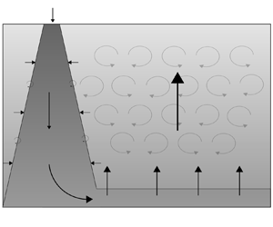
We model (figure 2) the convective mixing of a finite volume of fluid in an enclosed space with a localised positive buoyancy flux and a distributed negative buoyancy flux (where positive buoyancy in this context can be thought of as heavy fluid that sinks from the surface) at the surface of the reservoir. The fluid is Boussinesq, and we assume that there is an interior turbulence-driven eddy diffusivity that transports buoyancy. In the context of the oceans, there have been many studies aimed at quantifying this diffusion in terms of the local stratification, shear and external energy sources, such as that associated with the tides, but here we assume that this is a constant (Osborn Reference Osborn1980; Thorpe Reference Thorpe2005). We assume that a downwelling turbulent plume develops as described by the classical model of Morton, Taylor & Turner (Reference Morton, Taylor and Turner1956) for a plume with volume flux  ${\rm \pi} q$, momentum flux
 ${\rm \pi} m$ and buoyancy
 $b$, where the buoyancy is defined relative to a reference density, and here this is taken to be the mean density of the reservoir,
 $$\begin{gather} \bar{\rho} = \frac{1}{H}\int_0^{H} \hat{\rho} \,\mbox{d} z, \end{gather}$$
so that the depth-averaged buoyancy in the system is zero. It is possible to modify the details of the downwelling plume flow to represent a downslope gravity current, although the principles are similar for both types of downwelling flow (cf. Hughes & Griffiths Reference Hughes and Griffiths2006) as they entrain ambient fluid. To conserve mass, an upwelling flow develops in the interior. Guided by the models of Hughes et al. (Reference Hughes, Griffiths, Mullarney and Peterson2007) and Munk (Reference Munk1966), we assume that the downwelling flow has initial volume flux  ${\rm \pi} q _0$, initial momentum flux
 ${\rm \pi} m_0$, and a constant positive source buoyancy. We assume that the plume fluid returns to the surface in a uniformly distributed interior upwelling flow. In practice, there will be an adjustment zone between the laterally spreading plume fluid as it spreads over the reservoir floor and the overlying upwelling water (Whitehead & Wang Reference Whitehead and Wang2008), but in this work we assume that this boundary layer is very thin.
Schematic of the flow through a ventilated reservoir with an isolated destabilising (positive) source of buoyancy and a distributed stabilising (negative) buoyancy source along the surface with localised interior turbulent mixing.

In steady state, there is an equal and opposite flux of buoyancy in the plume and the remainder of the reservoir, and this relation has the form
 \begin{equation} q(z,t)\,b(z,t) = \kappa A\,\frac{\partial {\hat{b}}}{\partial {z}} + q(z,t)\,\hat{b}(z,t), \end{equation}
where  $\hat {b}$ denotes the buoyancy of the ambient, whilst
 $b$ denotes the buoyancy of the plume,
 $\kappa$ is the turbulent diffusivity in the interior, and the area of the reservoir is
 ${\rm \pi} A$.
The model equations for the plume can be summarised as
 $$\begin{gather} \frac{\partial {q}}{\partial {z}} = 2 \epsilon m^{{1}/{2}}, \end{gather}$$
 $$\begin{gather}m\,\frac{\partial {m}}{\partial {z}} = q^{2} (b - \hat{b}), \end{gather}$$
 $$\begin{gather}\frac{\partial {[q(b - \hat{b})]}}{\partial {z}} ={-}q\, \frac{\partial {\hat{b}}}{\partial {z}}, \end{gather}$$
where  $\epsilon$ is the empirically determined entrainment coefficient. There has been a considerable amount of work carried out in which models for the variation of the entrainment coefficient in a turbulent plume have been developed as the flow evolves from being momentum dominated (jet-like) to mass flux dominated (lazy) relative to the ideal pure buoyancy-driven plume (Caulfield & Woods Reference Caulfield and Woods1995; Hunt & Kaye Reference Hunt and Kaye2001; Carazzo, Kaminski & Tait Reference Carazzo, Kaminski and Tait2006; Craske & van Reeuwijk Reference Craske and van Reeuwijk2015; Ciriello & Hunt Reference Ciriello and Hunt2020). However, given the simplicity of the present model, we approximate the entrainment coefficient as a constant
 $\epsilon = 0.1$ (Turner Reference Turner1986) corresponding to the value for a pure plume; while a more detailed parametrisation is possible, we have found that the structure of the density profile in the interior of the domain is similar to that using a constant entrainment coefficient, especially for source conditions close to that of a pure plume.
We can combine (2.2) and (2.3c) to show that in steady state,
 \begin{equation} q(b- \hat{b}) = \kappa A\,\frac{\partial {\hat{b}}}{\partial {z}}\quad {\Rightarrow}\quad \frac{\partial {[q(b-\hat{b})]}}{\partial {z}} ={-}\kappa Aq^{2}(b - \hat{b}).\end{equation}
In this case, the specific buoyancy flux advected downwards by the plume is balanced directly by the upward diffusive flux of buoyancy in the interior, and both these quantities decrease monotonically from the surface. The boundary conditions for the plume volume flux, momentum flux and buoyancy are
 \begin{equation} q(0,t) = q_0,\quad m(0,t) = m_0,\quad b(0,t) = b_{p}. \end{equation}
2.1. Non-dimensionalisation
We scale the parameters using the buoyancy flux  $B_0 = q_0gb_{p}$ and the reservoir depth
 $H$, leading to the dimensionless properties (uppercase letters)
 \begin{equation} z = HZ,\quad b = b_{p}B. \end{equation}
In a point-source plume, Morton et al. (Reference Morton, Taylor and Turner1956) derived power-law solutions for the volume flux  $q$ and momentum flux
 $m$:
 \begin{align} q = \frac{4}{3}\left( \frac{9 \epsilon}{10}\right)^{4/3}B_0^{1/3}z^{5/3} \sim 0.054 B_0^{1/3}z^{5/3},\quad m = \left( \frac{9 \epsilon}{10} \right)^{2/3}B_0^{2/3}z^{4/3} \sim 0.2 B_0^{2/3}z^{4/3}. \end{align}
A plume with a finite mass flux at the source evolves as a pure buoyancy-driven plume if the source momentum flux satisfies the relation
 \begin{equation} m_0 = \left( \frac{5}{8 \epsilon}\,B_0 q_0^{2} \right)^{2/5}. \end{equation}
We therefore scale the plume volume flux  $q$ according to the power-law relation (2.7a,b) with
 $z = H$, and the momentum flux
 $m$ using the pure plume balance (2.8):
 \begin{equation} q = B_0^{1/3}H^{5/3}Q,\quad m = \left( \frac{5}{8 \epsilon}\,B_0 q_0^{2} \right)^{2/5} M. \end{equation}
Equations (2.3) and (2.4), and boundary conditions (2.5a–c), become
 $$\begin{gather} \frac{\partial {Q}}{\partial {Z}} = \left(20 \epsilon^{4} \right)^{1/5} \mathcal{R}^{-({2}/{5})} M^{{1}/{2}}, \end{gather}$$
 $$\begin{gather}M\,\frac{\partial {M}}{\partial {Z}} = \left( \frac{8 \epsilon}{5}\right)^{4/5}\mathcal{R}^{13/5} Q^{2} (B - \hat{B}), \end{gather}$$
 $$\begin{gather}\frac{\partial {\bigl[Q(B - \hat{B})\bigr]}}{\partial {Z}} ={-}\mathcal{R}\,Pe\,Q^{2}(B - \hat{B}), \end{gather}$$
 $$\begin{gather}Q(0,T) = \mathcal{R}^{{-}1},\quad M(0,T) = M_0,\quad B(0,T) = 1, \end{gather}$$
 $$\begin{gather}0 = \int_0^{1} \hat{B}\,\mbox{d} Z, \end{gather}$$
where  $M_0 = 1$ if at the source the plume is in pure plume balance. The two dimensionless parameters
 $\mathcal {R}$ and
 $Pe$ are given by
 \begin{equation} \mathcal{R} = \frac{B_0^{1/3}H^{5/3}}{q_0},\quad Pe = \frac{q_0 H}{\kappa A}. \end{equation}
Here,  $\mathcal {R}$ provides a scaling for the ratio of flux entrained by the plume over the depth of the domain,
 $B^{{1}/{3}}H^{{5}/{3}}$, to the source volume flux in the plume,
 $q_0$ (Morton et al. Reference Morton, Taylor and Turner1956). In the case
 $\mathcal {R} = {O}(10)$, the final volume flux has similar contributions from the initial source volume flux and the total volume flux gained from entrainment. The parameter
 $Pe$ represents a ratio for the scaling of the buoyancy transport associated with the plume source volume flux,
 $q_0 g b_p$, to the scaling for the diffusive transport of the buoyancy,
 ${g b_p \kappa A}/{H}$, over the whole area of the system.
In pure plume balance,  $M_0 = 1$ at the plume source, and the non-dimensional plume source radius
 ${r}/{H} = {q_0}/{H \sqrt {m_0}}$ is given by
 $(({8 \epsilon }/{5})({1}/{\mathcal {R}^{3}}))^{1/5}$. In all subsequent calculations, the plume source radius is taken to be constant with
 ${r}/{H} \sim 0.17$, so that the plume is in a pure buoyancy-driven balance at the source if
 $\mathcal {R} = 10$; in this case, the magnitude of the volume flux associated with entrainment is comparable to the volume flux from the plume source and is intermediate between the models presented by Munk (Reference Munk1966) and Hughes et al. (Reference Hughes, Griffiths, Mullarney and Peterson2007). In general, the dimensionless source momentum flux is
 $M(0,T) = ({10}/{\mathcal {R}})^{6/5}$. Additional calculations suggest that the qualitative results are similar to those presented herein even if the entrainment coefficient varies with the dimensionless momentum flux (cf. Ciriello & Hunt Reference Ciriello and Hunt2020), but for simplicity we keep the entrainment coefficient constant in the present work.
The limit  $\mathcal {R} \gg 10$ corresponds to the model presented by Hughes et al. (Reference Hughes, Griffiths, Mullarney and Peterson2007), who had a very small plume source volume flux initial condition. In contrast, the model of Munk (Reference Munk1966) is recovered in the case
 $\mathcal {R} \ll 10$.
In figure 3, we illustrate solutions in the cases  $Pe = 10$,
 $\mathcal {R} = 1$ (figure 3a),
 $Pe = 10$,
 $\mathcal {R} = 100$ (figure 3b),
 $Pe = 0.1$,
 $\mathcal {R} = 1$ (figure 3c) and
 $Pe = 0.1$,
 $\mathcal {R} = 100$ (figure 3d).
Overview of steady-state stratifications for combinations of small and large  $\mathcal {R}$ and
 $\mathit {Pe}$. Each panel shows a buoyancy profile for the plume and ambient, a plume volume flux profile, and a corresponding cartoon schematic for flow transport. Advective fluxes and diffusive fluxes are represented by straight and wavy arrows, respectively. Here,
 $Pe = 10, 0.1$ represent relatively weak and strong ratios of diffusive to source advective flux, and
 $\mathcal {R} = 1, 100$ represent relatively weak and strong ratios of entrained to source plume fluid.

Figure 3(a) corresponds to large  $Pe$ and small
 $\mathcal {R}$, so the interior diffusive flux is smaller than the source volume flux in the plume, while the transport in the plume is dominated by the source volume flux. In this case, there is a strong gradient of buoyancy in the upper reservoir, so as to match the surface buoyancy flux in the downwelling plume. However, the volume flux in the plume is nearly constant, so the buoyancy in the plume also remains nearly constant with depth. As a result, the source volume flux controls the buoyancy of the deep reservoir fluid.
In the case that  $\mathcal {R}$ and
 $Pe$ are large (figure 3b), there is again a region of strong stratification in the upper reservoir. However, now the plume entrains a significant volume of upper reservoir fluid, and this leads to a decrease in the plume buoyancy. However, once the plume fluid moves lower into the reservoir, below the stratified zone, the plume buoyancy does not evolve further with depth, even though it entrains more fluid. As a result, the mixing into the plume again strongly influences the buoyancy of the deep reservoir fluid where the buoyancy is constant with depth.
In the case of small  $Pe$, and small
 $\mathcal {R}$ (figure 3c), the diffusive flux in the reservoir is larger than the source volume flux in the plume, and this leads to a weak gradient of buoyancy across the depth of the reservoir. As the plume descends through the reservoir, it entrains some of this ambient fluid, and its buoyancy gradually falls. However, since the diffusive flux is so large, buoyancy diffuses out from the plume fluid supplied to the base of the reservoir, leading to a discrete drop in the buoyancy of the fluid at the base of the reservoir compared to the fluid supplied to the base of the reservoir by the plume, as given by the condition (2.10e). As a result, there is a weak gradient of buoyancy in the reservoir interior, while also in the downwelling plume.
Finally, in the case of small  $Pe$ and large
 $\mathcal {R}$ (figure 3d), the reservoir interior again has a small gradient of buoyancy. However, now the plume entrains much more ambient fluid, so the buoyancy in the plume decreases to smaller values as it descends to the bottom of the reservoir. There is still a jump in buoyancy at the base of the reservoir, with the interior water being less buoyant than the fluid supplied to the reservoir bottom by the plume. If
 $\mathcal {R}$ were to increase further, then the effects of entrainment would increase and the plume would eventually match the ambient buoyancy.
The two cases with  $\mathcal {R}$ small (figures 3a,c) correspond to scenarios where the entrainment is relatively weak and where the upwelling velocity is approximately constant, and these are consistent with the model presented by Munk (Reference Munk1966). The two cases with large
 $\mathcal {R}$ (figures 3b,d) correspond to scenarios where the entrainment is significant and the upwelling is strongly increasing with depth compared to the source volume flux, and these are consistent with the model presented by Hughes et al. (Reference Hughes, Griffiths, Mullarney and Peterson2007).
2.2. Regime classification
The different natures of the model predictions shown in figure 3 suggest that in some cases, the plume and deep reservoir water have essentially the same buoyancy (figures 3a,b), whereas in other cases, there is a jump in buoyancy at the reservoir floor (figure 3c). It is of interest to determine the critical conditions in  $(\mathcal {R}, Pe)$ space at which there is a transition from one regime to the other. Cases with a buoyancy jump between the plume and the reservoir arise when the diffusive flux extends over the entirety of the depth, whereas when the plume is of marginally greater buoyancy than the interior, the diffusion applies primarily in a boundary layer near the reservoir surface below which the descending plume is just driven primarily by its momentum.
We have determined the transition in regime systematically by mapping out the solutions in  $(\mathcal {R}, Pe)$ space and determining which solutions involve a jump in the buoyancy at the reservoir floor (figure 4). We distinguish the regimes by characterising a buoyancy jump if the difference in buoyancy between the plume and ambient at the base of the reservoir is
 $B(1) - \hat {B}(1) > \gamma = 0.01$, and in the case that there is a mixed layer, we determine the depth
 $H_m$ as the smallest
 $Z$ such that the jump in buoyancy is
 $B(Z) - \hat {B}(Z) < \gamma = 0.01$.
Overview of the different thresholds to characterise the plume and ambient stratifications. (a) Thresholds for a buoyancy jump in  $(\mathcal {R}, Pe)$ space defined as
 $B(Z) - \hat {B}(Z) \geq \gamma$, with
 $\gamma = 0.01$ (steel blue),
 $\gamma = 0.02$ (navy blue) and
 $\gamma = 0.04$ (indigo) at
 $Z=1$, and with
 $\gamma = 0.01$ at
 $Z = 0.9$ (ocean blue),
 $Z = 0.75$ (green) and
 $Z=0.6$ (turquoise). Three marked parameters correspond to the profiles in (b). (b) Plotted examples of the ambient (solid) and plume (dashed) buoyancy profiles at the critical thresholds. Colours of the profiles correspond with the thresholds in (a), with
 $\gamma = 0.04$ (indigo),
 $\gamma = 0.01$ (steel blue) at
 $Z=1$, and
 $\gamma = 0.01$ at
 $Z=0.6$ (turquoise).

In figure 4, we illustrate the locus of points in  $(\mathcal {R}, Pe)$ space on which the buoyancy jump at the reservoir floor has value
 $B(1) - \hat {B}(1) = \gamma$, where
 $\gamma = 0.01, 0.02, 0.04$. To illustrate the case in which there is a layer of nearly uniform buoyancy in the lowest part of the reservoir, we can show the locus of points in
 $(\mathcal {R}, Pe)$ space on which
 $B(Z) - \hat {B}(Z) = 0.01$ at dimensionless heights
 $Z=0.9, 0.75, 0.6$. Generally, it is seen that as
 $\mathcal {R}$ increases, the transition between these regimes occurs at progressively smaller values of
 $Pe$. This may be understood in that as
 $\mathcal {R}$ increases, there is more mixing of the deeper reservoir waters by the entrainment into plume, so a larger diffusive flux is required to cause a jump in the buoyancy at the reservoir floor. We see that the depth of the approximately well-mixed bottom layer quickly increases as the parameter
 $\mathcal {R}$ or
 $Pe$ increases. Similarly, the buoyancy jump at the reservoir floor increases quickly as
 $\mathcal {R}$ or
 $Pe$ decreases. In figure 5, we illustrate this effect by tracing loci through
 $(\mathcal {R}, Pe)$ space as the parameters
 $\mathcal {R}$,
 $Pe$ are varied independently. We also show the evolution of the system as the source volume flux
 $q_0$ varies, with other properties constant. Changing
 $q_0$ results in a change of both
 $\mathcal {R}$ and
 $Pe$, but provides a useful insight into the importance of the source volume flux on the evolution of the system. The different curves cross at
 $Pe \approx 1.6$,
 $\mathcal {R} \approx 35$. Along each curve, either the buoyancy profile has a jump at the reservoir floor, or instead the buoyancy is nearly uniform at the base of the reservoir. For
 $Pe$ small, the diffusive flux is stronger than the advective flux and we see a buoyancy jump occurring at the reservoir floor. As
 $Pe$ increases, the effects of diffusion weaken, and we see the stratification change into having a nearly uniform layer growing at the reservoir floor. A similar situation occurs for small
 $\mathcal {R}$, where a buoyancy jump occurs as the entrainment is weak here. As
 $\mathcal {R}$ increases, the entrainment of ambient fluid increases, and this results in the buoyancy jump decreasing in size until a nearly uniform layer forms. As
 $q_0$ changes, a combination of the above effects occurs since increasing
 $q_0$ changes the advection–diffusion balance whilst also changing the ratio of entrainment. We see that for large
 $q_0$, there is a nearly uniform layer that forms at the base of the reservoir since the stratification is controlled primarily by advection. As
 $Pe$ decreases, the relative effect of diffusion increases and the depth of the nearly uniform layer decreases until eventually
 $Pe \ll 1$ and a buoyancy jump at the reservoir floor occurs. As
 $Pe$ decreases further, the buoyancy jump reaches a maximum and then decreases again owing to the effects of entrainment becoming significant.
Overview of the changes in stratification as the parameters  $\mathcal {R}$ and
 $Pe$ change, measured as a transition from a buoyancy jump to a nearly uniform layer. (a) Loci in
 $(\mathcal {R}, Pe)$ space as
 $Pe$,
 $\mathcal {R}$ and source volume flux
 $q_0$ changes are illustrated corresponding to the other three panels. The regime transition threshold (light blue) of a buoyancy jump,
 $B(1) - \hat {B}(1) \geq 0.01$, as in figure 4 is also plotted. Variation in the buoyancy jump or well-mixed layer depth are plotted as functions of (b) plume source volume flux, (c) Péclet number
 $Pe$, and (d) entrainment ratio
 $\mathcal {R}$. Two points are highlighted by stars in (a,b), which are the parameter locations for the oscillations in § 3.

3. Transient evolution from steady state
The steady-state solutions provide insight into the controls in this idealised model of the stratification produced by the buoyancy-driven balance between the filling-box flow and the mixing produced by an interior diffusion of buoyancy. We now explore the impact of time-dependent perturbations in the surface buoyancy fluxes in order to understand how the system evolves from steady state. For simplicity, we examine the impact of an instantaneous change in the forcing as well as sinusoidal fluctuations in the forcing relative to a mean, and we examine the impact of both the frequency and magnitude of these fluctuations.
One challenge in the modelling concerns the case in which the source buoyancy flux decreases sufficiently rapidly that the plume is arrested by the stratification of the reservoir. In this case, the plume fluid will intrude at some intermediate level in the system. In the present model, we impose that the plume intrudes at the depth of neutral buoyancy, and that the fluid below this region participates in the buoyancy transfer only through the internal diffusivity, so there is no convective mixing in that zone. When this situation occurs, below the depth of neutral buoyancy the dynamics changes into that of a turbulent fountain (Bloomfield & Kerr Reference Bloomfield and Kerr2000); for simplicity in the present work, we neglect any effects of penetrative entrainment in this fountaining region.
In transient systems, the buoyancy fluxes in the plume and interior may not always be balanced, so independent boundary conditions need to be specified on the surface of the reservoir.
In ocean systems, surface buoyancy forcing occurs through a combination of heat and freshwater fluxes due to air–sea exchange, convection, ice formation and vertical mixing (Marshall & Plumb Reference Marshall and Plumb2007). This motivates categorising surface forcing into being (a) buoyancy-conserving in a ‘salt-like’ regime where the total salt in the system is constant, and (b) buoyancy-changing in a ‘heat-like’ regime where the net buoyancy may increase or decrease from the equilibrium state owing to net heating or cooling. In both cases, a perturbation to the boundary condition results in a redistribution of the buoyancy relative to the mean, whilst additionally in case (b), there is also a net increase in the system buoyancy, which may be interpreted as a net heating or cooling. For the purposes of the calculations in this section, we keep the total buoyancy constant, so a buoyancy-conserving surface boundary condition is used as described in case (a), given by
 \begin{equation} \left.\left[\frac{1}{Pe}\,\frac{\partial {\hat{B}}}{\partial {Z}} = \mathcal{R}Q(B - \hat{B}) \right]\right|_{Z=0}. \end{equation}
The alternative choice of a ‘heat-like’ surface boundary condition is more complex to parametrise, as can be seen in similar work by Hughes et al. (Reference Hughes, Griffiths, Mullarney and Peterson2007) and Griffiths et al. (Reference Griffiths, Hughes and Gayen2013), and we discuss this further in § 4.
The evolution of the buoyancy of the plume has the form of (2.3c), i.e.
 \begin{equation} \frac{\partial {[ Q(B - \hat{B}) ]}}{\partial {Z}} ={-}Q\frac{\partial {\hat{B}}}{\partial {Z}}, \end{equation}
while the interior stratification evolves according to the diffusion equation, and using the dimensionless time scale based on the time for the fluid entrained by the plume to mix the fluid in the reservoir,  ${AH}/{B_0^{{1}/{3}}H^{5/3}}$, we find
 \begin{equation} \frac{\partial {\hat{B}}}{\partial {T}} - Q\,\frac{\partial {\hat{B}}}{\partial {Z}} = \frac{1}{\mathcal{R}\,Pe}\,\frac{\partial {\hat{B}}}{\partial {Z}}. \end{equation}
The time scale of response of the reservoir is given by the smallest mixing time for the system, where the mixing time may be controlled by the entrainment  $\tau = 1$, the source flow
 $\tau = \mathcal {R}$, or the diffusive mixing
 $\tau = \mathcal {R}\,Pe$.
To begin this section, we illustrate the differences between the cases where the plume buoyancy flux varies according to a change in the plume volume flux (figures 6a,b) or the source buoyancy of the plume fluid (figures 6c,d). We start with a steady-state system with  $\mathcal {R} = 10$ and
 $Pe = 10$, and perturb the system instantaneously by increasing the buoyancy flux in the plume to
 ${\rm \Delta} Q\,P(0,t) = 0.4 \mathcal {R}$ (figures 6a,c) or decreasing it to
 ${\rm \Delta} Q\,P(0,t) = -0.4\mathcal {R}$ (figures 6b,d).
Illustration of the transient evolution of the interior stratification as the plume buoyancy flux (a,c) decreases instantaneously,  $Q\,B(0,t) = 0.6\mathcal {R}$ or (b,d) increases instantaneously,
 $Q\,B(0,t) = 1.4 \mathcal {R}$. Initially, the stratification is the steady state with
 $\mathcal {R} = 10$ and
 $Pe = 10$. Colour corresponds to the buoyancy of the stratification minus that of the steady state, where yellow corresponds to a surplus of buoyancy relative to the final steady state. Overlain also is the plume intrusion depth (red dashed line). There are two cases in which (a,b) plume source volume flux is changing or (c,d) plume source buoyancy is changing, in the cases of buoyancy flux (a,c) decreasing or (b,d) increasing.

In figures 6(a) and 6(c), we plot a time series of the instantaneous stratification minus the final steady-state stratification in the case where the buoyancy flux decreases. In both cases, the plume behaves qualitatively similarly in becoming arrested by the stratification and intruding at an intermediate depth. In figure 6(a), the plume source volume flux is decreased and the weakening of the plume buoyancy due to entrainment of ambient fluid increases, and in this case the plume intrudes at an intermediate depth. This results in a buildup of buoyancy above the intrusion depth. We also see a large deficit in buoyancy at the surface, since in this case, the surface has adjusted to the changing boundary condition but the interior stratification has not. In figure 6(c), the plume buoyancy is changed instead of the volume flux, and as time evolves there is no longer a relative buildup of buoyancy just above the plume intrusion depth. Similar to figure 6(a), the surface boundary condition results in a buoyancy deficit at the surface, and we also see a surplus of buoyancy near the floor of the reservoir as the deep water becomes disconnected from the plume convection.
In figures 6(b) and 6(d), we plot the time series of the instantaneous stratification minus the final steady-state stratification in the two scenarios in the cases when the buoyancy flux is increasing, and here convection occurs in the entire domain. Both cases behave similarly in showing a front rising from the bottom of the reservoir as the box fills. We also see initially a surplus of buoyancy near the surface, and this signifies the deficit of buoyancy in the mixed zone of the interior; the buoyancy of this fluid asymptotes towards the steady state by entraining progressively more buoyant fluid.
In summary in these calculations, perturbing the system by changing the plume source volume flux or the plume buoyancy has similar effects on the stratification by redistributing the buoyancy, where changing the volume flux has secondary effects in changing the balance between the surface advection and diffusion.
3.1. Oscillatory forcing
In proceeding, we choose a salinity-like case where the interior surface boundary condition is chosen such that buoyancy is conserved in the system and we represent the fluctuations in the source volume flux by changing  $q(0, t)$ according to the relation
 \begin{equation} q(0,t) = q_0[1 + Q_{amp} \sin(\omega t) ]\quad {\Rightarrow}\quad Q(0, T) = \mathcal{R}^{{-}1}[ 1 + Q_{amp} \sin(\varOmega T) ]. \end{equation}
We examine the difference in the response in terms of the dimensionless frequency and amplitude,
 \begin{equation} F= \varOmega \tau,\quad Q_\text{amp}. \end{equation}
For small values of  $F$, the forcing has a very long period, so we expect the system to evolve through a series of quasi-steady states. However, as
 $F$ decreases, the system may evolve further from equilibrium.
As discussed in § 2.2, there are two generic cases to consider, in which (a) there is a buoyancy jump at the reservoir floor between the plume and the ambient, and (b) there is a basal layer in which the plume and the ambient are nearly uniform (cf. figure 5). In § 3.2, we consider the case in which the there is a well-mixed basal layer, and in § 3.3, we consider the case of a buoyancy jump.
3.2. Well-mixed layer regime
We investigate an oscillatory perturbation in the regime where the plume and ambient buoyancy are approximately uniform near the reservoir floor. Decreasing the source volume flux may perturb the buoyancy flux of the plume so that the plume is arrested by the stratification higher in the water column, leading to a transient period of partial convection. We use the parameters  $\mathcal {R} = 10$,
 $Pe = 10$ as described in § 2, and vary the frequency
 $\varOmega = 0.01, 0.1, 1$, as well as exploring variations in the amplitude of the oscillations
 $Q_{amp} = 0.2, 0.4, 0.6$.
The buoyancy contours for an example run are plotted in figure 7. As the source volume flux oscillates, the changes in the ambient buoyancy profile are clear near the surface, and the plume intrusion depth may also be seen to vary with time (red dashed line). As the source volume flux increases, the buoyancy contours thin at the surface as the diffusive boundary flux increases. We also see a displacement flow style filling from the reservoir floor with a single rising contour. As the source volume flux decreases, surface buoyancy contours widen in order to weaken the diffusive surface flux. The plume also begins to intrude at an intermediate depth and leads to a weakening of the stratification at that depth.
Overview of an example run within the well-mixed layer regime ( $\mathcal {R} = 10$,
 $Pe = 10$) with
 $\varOmega = 0.1$,
 $Q_{amp} = 0.4$. At the top, the blue and green lines are contours of
 $\hat {B}$ in a neighbourhood of
 $\hat {B} = 0$, with the red dashed line showing the plume intrusion depth. The bottom plot shows the corresponding oscillating source flux.

In figures 8(a,b), we plot the depth of the well-mixed region above the reservoir floor  $H_m$ for three values
 $\varOmega = 0.01, 0.1, 1$,
 $Q_{amp} = 0.4$ (figure 8a), and for
 $\varOmega = 0.1$,
 $Q_{amp} = 0.2, 0.4, 0.6$ (figure 8b), as a function of
 $Q(0, T)$. The oscillation converges to a clockwise loop in the
 $(q, H_m)$ space as
 $Q(0,T)$ oscillates. We note that
 $H_m$ is as defined in the text in § 2.2, determining the minimum depth such that the buoyancy difference between the plume and interior is sufficiently small. In a transient system, the layer of fluid below this depth is not always nearly well-mixed, but this measurement is still used to draw a comparison with the steady-state solutions. The locus of the smaller-frequency cycles
 $\varOmega = 10^{-2}$ follows the steady-state solutions loosely, but there are two solution branches for
 $H_m$ as a function of
 $Q(0,T)$, depending on whether
 $Q(0,T)$ is increasing or decreasing, whilst with the higher-frequency
 $\varOmega = 1$ forcing, the solution remains much more transient, and departs significantly from the steady state. The case with intermediate forcing,
 $\varOmega = 10^{-1}$, has a locus between the two described previously. As seen from § 2 and the steady-state line, an increasing volume flux increases the depth of the homogenised layer. In contrast to this, the behaviour in the high-frequency case,
 $\varOmega =1$, of a decreasing well-mixed layer depth arises owing to increasing plume source buoyancy flux since, on the time scale of the fluctuation, the ambient cannot adjust sufficiently rapidly. Changing the perturbation amplitude
 $Q_{amp}$ widens the amplitude of the perturbations but does not appear to make any qualitative changes to the shape of the cycles within the range of
 $Q_{amp}$ used.
Illustrations of the differences that occur in the well-mixed layer regime ( $\mathcal {R} = 10$,
 $Pe = 10$) between the steady state and with the inclusion of a sinusoidal oscillation with (a)
 $\varOmega = 0.01, 0.1, 1$,
 $Q_{amp}=0.4$, and (b)
 $\varOmega = 0.01$,
 $Q_{amp} = 0.3, 0.4, 0.5$. (a,b) Locus of the nearly well-mixed layer depth
 $H_m$ as the source volume flux
 ${q(0)}/{q_0}$ varies for three frequencies (blue–green), along with the reference steady-state locus (red). The nearly well-mixed layer depth
 $H_m$ is as defined in the text in § 2.2 and measures the relative buoyancy between the plume and the ambient; it is not necessarily well-mixed in this layer and vertically uniform due to the transience. (c–e) Time series of the subtraction of the instantaneous steady-state profiles from the solution for three frequencies (
 $\varOmega = 0.01, 0.1, 1$), with yellow being a relative excess of buoyancy compared to the steady-state profile, and blue a deficit, along with the depth of neutral buoyancy (red dashed line). Note that the magnitude of relative buoyancy represented in false colour in each of the three figures is changing.

To help to clarify the process, in figures 8(c–e) we present images showing the time evolution of the buoyancy relative to the steady-state buoyancy, at each depth in the system. The colours show an increase (yellow) and decrease (blue) in the buoyancy. The general trend is that the higher-frequency oscillations result in a greater evolution from the steady state compared to the lower-frequency oscillations. In figure 8(c), we see a buildup of surface buoyancy as the volume flux increases, and a deficit as the volume flux decreases. As the volume flux decreases and the plume intrudes at an intermediate height, we also see an excess of buoyancy just above this height. This behaviour arises because the flow is in an advection-dominated regime; the surface responds to changing surface boundary conditions, but the steady state is achieved when there is a balance between advective and diffusive fluxes, and here we have an effective buoyancy deficit since the denser deep water is disconnected from the convection. This buoyancy is transferred back into the convection through the relatively weaker diffusion.
3.3. Buoyancy jump regime
Here, we investigate the oscillations in the alternative regime where there is a buoyancy discontinuity at the reservoir floor. Similar parameters are used as in § 3.2 with the exception that the plume source volume flux is thirty times smaller than previously used, resulting in  $\mathcal {R} = 10 \times 30^{2/3} = 96.5$ and
 $Pe = \frac {10}{30} = 0.333$. This shifts us into the more diffusive regime, with a buoyancy jump at the base of the reservoir. In this case, a larger perturbation will be required for the plume to be arrested by the stratification. (cf. figure 5). We apply the linear perturbation of the form of (3.4).
The buoyancy contours of an example run can be seen in figure 9. As the source volume flux oscillates, we see a uniform contraction and expansion of the buoyancy contours across the entire domain. This is contrasted with figure 7, in which, as the volume flux increased, there was an asymmetric diffusive sharpening that was most apparent in the surface boundary layer.
Overview of an example run within the buoyancy jump regime ( $\mathcal {R} = 10 \times 30^{2/3}$,
 $Pe = \frac {10}{30}$) with
 $\varOmega = 0.1$,
 $Q_{amp} = 0.3$. At the top, the blue and green lines are contours of
 $\hat {B}$ in a neighbourhood of
 $\hat {B} = 0$, with the red dashed line showing the plume intrusion depth. The bottom plot shows the corresponding source volume flux for reference.

In figures 10(a) and 10(b), we illustrate the variation with source volume flux of the magnitude of the density jump at the base of the reservoir as a function of the frequency  $\varOmega$ and perturbation amplitude
 $Q_{amp}$. The oscillation in the source volume flux traces an anticlockwise locus in this space. Analogous to § 3.2, with the lower-frequency forcing, the solution locus follows the steady state closely, whilst the higher-frequency solution evolves far from the equilibrium solution. In the case of a higher frequency, the increasing volume flux results in the plume retaining more of its original buoyancy when it reaches the reservoir floor, whilst the ambient has not yet adjusted to the increasing buoyancy supplied by the plume. As the volume flux decreases, the effects of entrainment are greater, so the plume has less buoyancy, and at the reservoir bottom, the ambient has relatively more buoyancy than in steady state, so the buoyancy discontinuity becomes smaller. Varying the oscillation amplitude
 $Q_{amp}$ changes the magnitude of the difference in buoyancy of the locus traced but makes no significant qualitative difference.
Illustrations of the differences that occur in the buoyancy jump regime ( $\mathcal {R} = 10 \times 30^{2/3}$,
 $Pe = \frac {10}{30}$) between the steady state and with the inclusion of a sinusoidal oscillation with (a)
 $\varOmega = 0.01, 0.1, 1$,
 $Q_{amp}=0.3$, and (b)
 $\varOmega = 0.01$,
 $Q_{amp} = 0.2, 0.3, 0.4$. (a,b) Locus of the buoyancy difference between the plume and ambient at
 $Z=1$ as the source volume flux
 ${q(0)}/{q_0}$ varies for three frequencies (blue–green), along with the reference steady-state locus (red). (c–e) Time series of the subtraction of the instantaneous steady-state profiles from the solution for three frequencies (
 $\varOmega = 0.01, 0.1, 1$), with yellow being a relative excess of buoyancy compared to the steady profile, and blue a deficit, along with the depth of neutral buoyancy (red dashed line). Note that the magnitude of relative buoyancy represented in false colour in each of the three figures is changing.

In figures 10(c–e), we illustrate the difference in the buoyancy at each depth of the reservoir relative to the buoyancy of the steady-state solution, as a function of time. The colours show an increase (yellow) and decrease (blue) in the buoyancy at each point. The profiles with higher-frequency oscillations have a larger deviation from the steady state, and the plume intrusion always occurs at the reservoir floor within the chosen parameter range. The deviation occurs in a somewhat symmetric manner between the reservoir surface and floor within all frequencies shown in the figure, corresponding to a steepening or shallowing of the buoyancy gradient, and hence buoyancy variation across the reservoir as the source volume flux decreases or increases.
4. Discussion
We have investigated a simplified model of a ventilated, diffusive filling-box. We account for a positively buoyant plume supplied with a finite volume flux at the surface balanced by a source of negative buoyancy distributed across the reservoir surface, and present our equations and solutions in terms of  $\mathcal {R}$, the ratio of the entrained volume flux to the source volume flux, and
 $\mathit {Pe}$, the ratio of the source volume flux to the diffusive flux. We find that in steady state, there are scenarios with large
 $\mathcal {R}$ or large
 $Pe$ where there is a surface diffusive boundary layer but the deep reservoir is well-mixed as a result of entrainment and recirculation from the plume. in cases with small
 $Pe$, the reservoir waters are linearly stratified. A key result is that the ratio of transport of buoyancy associated with the source plume advection compared to the interior diffusive transport of buoyancy is important since the interior buoyancy stratification is set by the buoyancy decay near the surface, (2.4) and (2.10c), and to leading order this is dependent on the plume source volume flux
 $q_0$. Including the plume source volume flux bridges the gap between the Munk (Reference Munk1966) model, where no entrainment occurs and the source volume flux dominates, and the Hughes et al. (Reference Hughes, Griffiths, Mullarney and Peterson2007) model, where the downwelling plume volume flux is the result of entrainment exclusively. The simplification to model the downwelling convection as a traditional plume (Morton et al. Reference Morton, Taylor and Turner1956) was suggested first by Munk (Reference Munk1966) and used subsequently by Hughes et al. (Reference Hughes, Griffiths, Mullarney and Peterson2007). The present model is heavily idealised but follows on from the work of Hughes et al. (Reference Hughes, Griffiths, Mullarney and Peterson2007). In future work it would be interesting to: alter the details of the downwelling convection by modelling it as a line plume or as a gravity current (Hughes & Griffiths Reference Hughes and Griffiths2006); include variations of the ratio of the plume source radius to the reservoir depth; and also test the inclusion of the detailed change in the entrainment coefficient as a function of the deviation from pure plume behaviour (Ciriello & Hunt Reference Ciriello and Hunt2020).
Instant changes in the plume buoyancy forcing show that the response time depends on the shorter of the ventilation and diffusive mixing times in the reservoir, with the system readjusting to a new equilibrium over this time. If the plume source volume flux varies in time, then the dynamics of the plume and the buoyancy structure of the plume evolves according to whether the time scale of the oscillation is relatively small compared to the ventilation and the diffusive mixing time of the reservoir. In the case of a short time scale of change, the system exhibits inertia and lags behind in adjusting to the changing forcing conditions, and the stratification is not representative of the instantly changing forcing conditions. If the time scale is relatively large, then the system retains the stratification in a quasi-steady regime but along a loop where the pathway taken is different depending on if the volume flux is increasing or decreasing. In an advection-dominated regime where there is a well-mixed layer at the reservoir floor, with a sufficiently large perturbation, the plume may no longer be able to penetrate into the deep, and limited circulation occurs in the upper reservoir. This may indicate major changes in the convective circulation pattern with sufficiently rapid or high magnitude forcing to the system. As the plume flux eventually increases again, the plume is able to re-enter the deep reservoir. The deviation from steady state has bigger amplitude signals near the surface, and the changes to the stratification here respond more rapidly, whilst the deviations below the surface diffusive layer are smaller and more vertically distributed. The deviation is indicative of advective behaviour where fluid must upwell through the entirety of the reservoir depth before balancing the surface diffusion. In the case of a diffusively dominated regime, this equilibration occurs uniformly and symmetrically.
4.1. Physical interpretation
The results here may provide some insight into some of the processes at play in the deep thermohaline circulation of the ocean if the forcing at the surface changes. Here, we input some physical parameters into the model to see the implications for the world oceans, but noting the simplicity of the model. From Orsi, Johnson & Bullister (Reference Orsi, Johnson and Bullister1999), we use a plume source volume flux by taking the source of bottom water production, agreed in the literature as ‘Weddell Sea Bottom Water’, and this has value  $3 \times 10^{6}\,\text {m}^{3}\,\text {s}^{-1}$. From Munk (Reference Munk1966), we use values for the basin horizontal area
 $A = 1.37\times 10^{14}\,\text {m}^{2}$, as well as motivations for the Péclet number
 $Pe_{Munk} = 3.3$ (after notational adjustments), where
 $Pe$ is the important parameter controlling the depth of the surface pycnocline. We note that in defining
 $Pe$, Munk (Reference Munk1966) uses a constant value representing the volume flux at the bottom of the ocean, which Munk (Reference Munk1966) estimates as
 $19 \times 10^{6}\,\text {m}^{3}\,\text {s}^{-1}$, and Orsi et al. (Reference Orsi, Johnson and Bullister1999) estimate at
 ${\sim }10\unicode{x2013}15\times 10^{6}\,\text {m}^{3}\,\text {s}^{-1}$. For the present model, we require the value near the upper part of the deep thermohaline circulation. To achieve the value
 $Pe = 3.3$, keeping the ratio
 ${q_0 H}/{\kappa A}$ fixed and using the source volume flux, Munk's value
 $\kappa = 1.3 \times 10^{-4}\,\text {m}^{2}\,\text {s}^{-1}$ must be scaled appropriately, so we use diffusivity
 $\kappa \sim 2 \times 10^{-5}\,\text {m}^{2}\,\text {s}^{-1}$, and this is consistent with more recent interior diffusivity measurements (Polzin et al. Reference Polzin, Toole, Ledwell and Schmitt1997; Ledwell, Watson & Law Reference Ledwell, Watson and Law1998). Finally, the values for the haline expansion coefficient
 $\beta = 8 \times 10^{-4}$, the mean salinity
 $\bar {S} = 34\,\text {g}\,\text {kg}^{-1}$ and the depth of the ocean
 $H = 4 \times 10^{3}\,\text {m}$ are taken from Klinger & Haine (Reference Klinger and Haine2019); the plume salinity
 $s_p = 34.7\,\text {g}\,\text {kg}^{-1}$ is taken from Foster & Carmack (Reference Foster and Carmack1976b), and for the purposes of this simple illustration, we assume that the salinity controls primarily the buoyancy in the system. These values are summarised in table 1, and although highly simplified, this suggests that the ocean today has approximate values
 $Pe \sim 4$,
 $\mathcal {R} \sim 9$, so the results from § 3.2 may be applicable and the frequencies
 $\varOmega = 0.01, 0.1, 1$ correspond roughly to a dimensional
 $\omega = 0.2 \times 10^{-2},\ 0.2 \times 10^{-3},\ 0.2 \times 10^{-4}\ \text {years}^{-1}$.
Sample ocean parameter values, taken from Munk (Reference Munk1966), Foster & Carmack (Reference Foster and Carmack1976a), Klinger & Haine (Reference Klinger and Haine2019) and Orsi et al. (Reference Orsi, Johnson and Bullister1999).

Surface forcings on the system may drift and vary with differing magnitudes over many different time scales related to the seasons, solar flare activity, anthropogenic emissions, and glacial to interglacial epochs (Hoyt Reference Hoyt1979; Sigman & Boyle Reference Sigman and Boyle2000; Rosenzweig et al. Reference Rosenzweig2008). If a sinusoidal variation of the boundary conditions is applied with frequency  $\varOmega = 0.01$ (period of order 50 000 years), such as Milankovitch cycles related to oscillations in the eccentricity of the planet's orbit as well as obliquity and precession of the orbit, then the present model calculations suggest that there may be some inertia in the response of the ocean to the forcing, but the overall pattern of circulation persists in a quasi-steady regime. In contrast, a shorter-period forcing with frequency
 $\varOmega = 1$ (period of order 500 years), perhaps related to climate change or other impulsive forcing, has a period much shorter than that of the adjustment time of the ocean, and if this change results in a decrease in the buoyancy flux in the poles, then it may lead to the plume intruding at an intermediate height, and separation of the deep ocean water from the overlying plume convection. It may be of interest to explore such changes in the forcing using a more detailed numerical simulation from an ocean general circulation model.
In § 3, we chose to use a buoyancy-conserving boundary condition for the calculations in order to study parametrically the transient evolution of an interior stratification subject to perturbations in the forcing. The buoyancy-conserving boundary condition allows for these effects to be isolated without worrying about the effects of the reservoir-integrated buoyancy changing or about specifying the parametrisation of the surface heat exchange. A common approach is to approximate the radiative fluxes and conductive transfers as a restoring force such that the heat flux  $Q$ may be approximated by (Haney Reference Haney1971; Rahmstorf & Willebrand Reference Rahmstorf and Willebrand1995)
 \begin{equation} Q = \lambda \left( T_\star{-} T_S \right), \end{equation}
where  $T_S$ is the surface temperature,
 $T_\star$ is the the target temperature, and
 $\lambda$ is the constant of proportionality. It would be interesting to explore the effects of such a boundary condition and the associated net change in buoyancy in further development of the work.
Declaration of interests
The authors report no conflict of interest.


 Open access

