


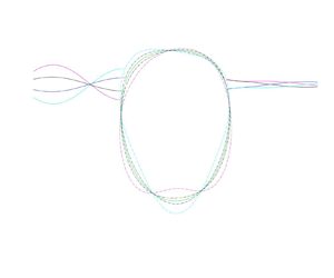

1. Introduction
Since the early 1990s, the use of membrane structures in the marine environment has become a trend (Ohyama et al. Reference Ohyama, Tanaka, Kiyokawa, Uda and Murai1989; Koley et al. Reference Koley, Vijay, Nishad and Sundaravadivelu2022). According to the difference between the membrane shapes, they can be divided into linear and arcuate membranes. While the linear membrane refers to the membrane in the natural state or the linear structure formed by tension on both sides (Kim & Kee Reference Kim and Kee1996; Williams Reference Williams1996), and arcuate membrane refers to the membrane that forms a closed space, which is filled with a liquid or gas to make it expand (Phadke & Cheung Reference Phadke and Cheung2003; Zhao et al. Reference Zhao, Zhou, Zong, Yang and Luo2022). In particular, fluid-filled membrane structures, which are composed of an arcuate membrane, have a wider range of potential applications. On the one hand, they can be used as a temporary offshore structure for wave attenuation, such as floating fluid-filled membrane breakwater (FFMB) and submerged fluid-filled membrane breakwater (SFMB) (Broderick & Jenkins Reference Broderick and Jenkins1993; Phadke & Cheung Reference Phadke and Cheung1999, Reference Phadke and Cheung2001). On the other hand, they can be used as a flexible pipeline designed to carry and transport oil and other liquids lighter than water (Zhao Reference Zhao1995). Moreover, a fluid-filled flexible tube can also be used for wave power absorption, such as the Anaconda wave energy converter (Babarit et al. Reference Babarit, Singh, Mélis, Wattez and Jean2017; Kurniawan et al. Reference Kurniawan, Chaplin, Greaves and Hann2017). Because these membrane structures are flexible, easy to handle, portable and reusable, environmentally friendly in the ocean, easily recycled and inexpensive to construct (Sahoo Reference Sahoo2012; Koley & Sahoo Reference Koley and Sahoo2017a; Li et al. Reference Li, Liu, Li and Fang2020), it is of great engineering application value to use flexible fluid-filled structures in the sea, especially for breakwaters.
Unlike traditional rigid breakwaters (Christensen et al. Reference Christensen, Bingham, Friis, Larsen and Jensen2018; Lv & Zhao Reference Lv and Zhao2021; Cheng et al. Reference Cheng, Fu, Dai, Collu, Ji, Yuan and Incecik2022; Ning et al. Reference Ning, Zhang, Chen, Liu and Teng2022), the interaction between the membrane breakwaters and waves is a complex dynamic process (Zhao & Aarsnes Reference Zhao and Aarsnes1998). The membrane structure will be greatly deformed under the action of waves, and the interaction between radiated waves and scattered waves can shield the water behind the breakwater (Cho & Kim Reference Cho and Kim1998; Koley, Behera & Sahoo Reference Koley, Behera and Sahoo2015). The successful realization of these systems requires accurate modelling and analysis of the waves on and around the membrane and the stress and strain in the material (Liu & Huang Reference Liu and Huang2019). Therefore, it is of great significance to analyse the hydrodynamic performance of membrane structure and explore their mechanism, so as to provide a theoretical basis for engineering practice.
Since the linear membrane breakwaters are relatively easier to handle than that of the arcuate membrane, numerous researchers have dedicated their efforts to studying their hydrodynamic performance under waves (Sahoo Reference Sahoo2012; Koley et al. Reference Koley, Behera and Sahoo2015; Mandal & Sahoo Reference Mandal and Sahoo2016). Williams (Reference Williams1996) developed a model of a pre-stretched thin membrane using the eigenfunction expansion method, and subsequently provided a numerical solution to the problem by employing the source distribution method. The researchers discovered that the wave reflection was primarily influenced by the membrane length, the weight of the mass and the mooring stiffness, while the membrane weight and the buoyancy of the system exerted a relatively minor effect. Based on the eigenfunction expansion method, some scholars have conducted relevant studies on vertical pre-stretched membranes (Kim & Kee Reference Kim and Kee1996; Williams Reference Williams1996; Kee & Kim Reference Kee and Kim1997; Lo Reference Lo2000) and horizontal membranes (Cho & Kim Reference Cho and Kim1998; Karmakar & Sahoo Reference Karmakar and Sahoo2008). The results demonstrate that the superposition of radiated and scattered waves generated by membrane motion results in wave attenuation. Furthermore, the width, position and tension of the membrane are identified as crucial factors. Moreover, some researchers have demonstrated that open-aperture membranes exhibit superior wave attenuation effects (Kumar, Manam & Sahoo Reference Kumar, Manam and Sahoo2007; Koley & Sahoo Reference Koley and Sahoo2017a,Reference Koley and Sahoob; Koley et al. Reference Koley, Vijay, Nishad and Sundaravadivelu2022). By adjusting factors such as the length, stiffness, permeability, layer number and tension of the membrane (Karmakar, Bhattacharjee & Soares Reference Karmakar, Bhattacharjee and Soares2013; Koley & Sahoo Reference Koley and Sahoo2017b), as well as the type of mooring (Kee Reference Kee2005), the breakwater can have a good effect on wave attenuation.
For the arcuate membrane, according to the different positions of the fluid-filled membrane breakwater, the breakwaters can be divided into FFMB and SFMB. For the SFMB, Ohyama et al. (Reference Ohyama, Tanaka, Kiyokawa, Uda and Murai1989) developed a linear model of the SFMB and compared their numerical results with experimental data, focusing on the wave transmission and reflection coefficients. Phadke & Cheung (Reference Phadke and Cheung1999), Phadke & Cheung (Reference Phadke and Cheung2003) derived a governing equation based on the thin membrane theory of cylindrical thin shells, obtained the kinematic response of the SFMB preliminary by using the boundary element method. Das & Cheung (Reference Das and Cheung2009) used a boundary element method coupled with a finite element model to study the three-dimensional response of an SFMB in a wave flume. Liu & Huang (Reference Liu and Huang2019) used the mixed Euler–Lagrange model to simulate the interaction between nonlinear waves and the SFMB, focusing on the kinematic response of the SFMB and related nonlinear wave scattering. Based on the potential flow theory and multipole expansions, Li et al. (Reference Li, Liu, Li and Fang2020) studied the interaction between the water wave and the SFMB through theoretical analysis, and analysed the effects of internal pressure and structural height on the wave transmission and reflection coefficients. Zhao et al. (Reference Zhao, Zhou, Zong, Yang and Luo2022) used computational fluid dynamics to study the interaction between waves and the SFMB. The overpressure, vorticity field, elastic modulus and structural response are analysed, and three different vibration modes of membrane structure under different wave frequencies are determined.
For the FFMB, Broderick & Jenkins (Reference Broderick and Jenkins1993) studied the interaction between a flexible underwater horizontal cylinder and surface waves, and compared the results with laboratory experiments. Broderick & Leonard (Reference Broderick and Leonard1995) proposed a time-domain model of nonlinear interaction between deformable objects and waves. In their method, the boundary element model of external fluid is coupled with the finite element model of the membrane. The internal fluid is not modelled and the internal pressure is assumed to be constant. Zhao (Reference Zhao1995) adopted the control equation based on the circumferential tension and the pressure difference balance between the two sides of the membrane to study the dynamic response of a floating fluid-filled membrane. Zhao & Aarsnes (Reference Zhao and Aarsnes1998) later expanded the model to include membrane elasticity and compared their numerical results with experimental data. Based on the principle of virtual work, Phadke & Cheung (Reference Phadke and Cheung2001) derived the variational governing integral equation of thin membrane deformation. Coupling two boundary element models with the finite element model of the membrane structure, the potential flow solutions of the internal and external fluids is obtained, and the vibration characteristics of the membrane structure are given.
The aforementioned research has thoroughly analysed the law of interaction between waves and the FFMB, thereby providing invaluable results for practical application. However, up to now, in these studies, the membrane has been modelled as a stretched straight string, in which the lateral displacement satisfies a one-dimensional wave equation (Kim & Kee Reference Kim and Kee1996; Kee & Kim Reference Kee and Kim1997; Karmakar & Sahoo Reference Karmakar and Sahoo2008; Mandal & Sahoo Reference Mandal and Sahoo2016; Koley & Sahoo Reference Koley and Sahoo2017b; Koley et al. Reference Koley, Vijay, Nishad and Sundaravadivelu2022), and the effect of the membrane curvature has not been considered. Therefore, the motion of the arcuate membrane cannot be accurately predicted through the one-dimensional equation, and the motion response of FFMB under wave action can not be accurately described. In addition, although some numerical studies have been carried out on the FFMB, there are few experimental studies on it, especially on its transmission coefficient, reflection coefficient, wave force and the response to FFMB, which also limit the application of FFMB in engineering.
This paper presents a general motion equation for both arcuate and linear membranes. It is used as the dynamic boundary condition of a two-dimensional thin membrane, which overcomes the difficulty of coupling the motion of arcuate membranes from the flow field in existing models. Then, a coupled eigenfunction expansion boundary element method (EEBEM) (Lv, Zhao & Li Reference Lv, Zhao and Li2022) and water flume experiments are used to comprehensively study the hydrodynamic performance of the FFMB, which complements the lack of existing experimental data and demonstrates the kinematic response of the FFMB. The EEBEM is a method that combines the eigenfunction expansion method with the multi-domain boundary element method (Chen et al. Reference Chen, Yueh, Chang and Wen2017; Zhao et al. Reference Zhao, Liu, Li and Chang2020). By coupling the corresponding boundary conditions at the boundaries of adjacent regions, the interaction between arbitrary structures and waves can be fully realized. At the same time, compared with the traditional multi-domain boundary element method (Bakhti et al. Reference Bakhti, Chioukh, Hamoudi and Boukhari2017), the eigenfunction expansion method can effectively reduce the computational domain, improve the computational speed and achieve higher numerical accuracy. Finally, the structural parameters suitable for practical engineering waters are proposed to provide a reference for engineering applications.
The remainder of this paper is structured as follows. Section 2 describes in detail the derivation of the membrane's motion equation and the realization of the EEBEM. Then, the FFMB model is briefly introduced in § 3, and the interaction between waves and the FFMB is revealed through the EEBEM and experimental results, with emphasis on the analysis of nonlinear waves and motion response. In § 4 the hydrodynamic performance of the FFMB is demonstrated by the EEBEM, and the influence of the FFMB density, filling ratio, radius and elastic modulus is emphatically analysed. The structural parameters applicable to engineering practice are given. Finally, the main conclusions are given in § 5.
2. Hydrodynamic formulation and EEBEM
2.1. Static boundary conditions of the FFMB
Figure 1 shows the sketch of an FFMB, in which the  $x$ axis is the still water surface and the
 $z$ axis is upward. The FFMB is composed of membrane and internal fluid, in which the membrane density is
 $\rho _s$ and the membrane thickness is
 $\varDelta$. The fluid density inside and outside of the membrane are
 $\rho _I$ and
 $\rho _O$, respectively, satisfying
 $\rho _I<\rho _O$. As a result, the FFMB floats on the water surface due to the buoyancy. Here
 $\theta$ represents the angle between the tangent of the membrane and the positive direction of the
 $x$ axis;
 $z = z_h$ and
 $z = -z_b$ denote the vertical positions of the highest and lowest points of the FFMB, respectively;
 $S$ represents the length of the membrane extending clockwise from the apex
 $(0,z_h)$;
 $p_{i0}$ represents the internal membrane pressure of the FFMB and
 $T_S$ represents the initial static tension of the FFMB. The static shape of the FFMB depends on the filling ratio
 $\gamma$ and the relative density
 $\rho _I/\rho _O$ of the fluid inside and outside the membrane.
Schematic diagram of wave with the FFMB.

The filling ratio  $\gamma$ is defined as
 \begin{equation} \gamma = A_0/A_{max}, \end{equation}
where  $A_0$ is the area surrounded by the membrane and
 $A_{max}$ is the largest possible area for which the membrane shape is circular. When the filling ratio is
 $\gamma = 1$, the geometry of the membrane is circular (as shown in figure 3, blue line) and the radius of this circle is called the membrane radius
 $R_C$.
This paper briefly introduces the method of obtaining the static shape of the FFMB as follows. For more details, please refer to Zhao (Reference Zhao1995). As shown in figure 2, assuming that a small element of the membrane is  ${\rm d} S$, the initial membrane tension is
 $T$, the resultant force of internal and external fluid pressures is
 $p_n$, the tangential force on the membrane is
 $p_t$ and the deflection angle of the element is
 ${\rm d} {\theta }$. Since the membrane thickness is infinitely thin, the mass and gravity of the membrane can be neglected. The force balance equation of the membrane element can be written as
 \begin{equation} \left. \begin{array}{@{}c@{}} {{p_n}\, {\rm d} S = 2T\sin ({\rm d} \theta /2) + {\rm d} T\sin ({\rm d} \theta /2)}, \\ {{\rm d} T\cos ({\rm d} \theta /2) + {p_t}\, {\rm d} S = 0,} \end{array} \right\} \end{equation}
where
 \begin{equation} \left. \begin{array}{@{}ll@{}} {p_n} = {p_{i0}} + {\rho _I}g ({z_h} - z), & z \ge 0, \\ {p_n} = {p_{i0}} + {\rho_I}g ({z_h} - z) + {\rho_O}gz, & z < 0. \end{array} \right\} \end{equation}
Stress analysis of the FFMB.

Since the fluid is assumed to be inviscid, the friction force on the membrane is zero, that is,  ${{\partial T}}/{{\partial S}} = 0$. According to (2.2), the differential equation of the membrane can be expressed as
 \begin{equation} {{p_n}\,{\rm d} S = T\,{\rm d} \theta \Rightarrow \frac{1}{R} = \frac{{{\rm d} \theta }}{{{\rm d} S}} = \frac{{{p_n}}}{T},} \end{equation}
where  $R$ is the radius of curvature.
The static shape of the FFMB is symmetrical to the  $z$ axis. Therefore, for the highest
 $(0,z_h)$ and lowest points
 $(0,-z_b)$, the membrane needs to satisfy the following boundary conditions:
 \begin{equation} \left. \begin{array}{@{}ll@{}} \theta (S) = 0, & S = 0, \\ \theta (S) = {\rm \pi}, & S = {L_m}/2. \end{array} \right\} \end{equation}
Here  $L_m$ is the total length of the membrane.
Applying Taylor expansion to the membrane angle  $\theta (S)$ and substituting (2.4) into it, we can obtain
 \begin{equation} \theta ({S_j} + \Delta S) = \theta ({S_j}) + \frac{{{\rm d} \theta ({S_j})}}{{{\rm d} S}}\Delta S + \frac{{{{\rm d}^2}\theta ({S_j})}}{{{\rm d} {S^2}}}{(\Delta S)^2} + \cdots\simeq \theta ({S_j}) + \frac{{{p_n}}}{T}\Delta S. \end{equation}
According to (2.5) and (2.6), when the internal membrane pressure  $p_{i0}$ and the highest point
 $(0,z_h)$ of the FFMB are known, the curve of the membrane boundary can be obtained by arbitrarily assuming the membrane tension
 $T$ and membrane difference length
 $\Delta S$. However, because the tension is unique when the membrane is in equilibrium, the curve will not satisfy (2.5) when the assumed tension
 $T$ does not match the actual tension. Assuming that the actual tension is
 $T_S$, (2.5) is adopted as the discriminant condition, and the tension
 $T$ is iterated continuously until
 $T = T_S$, then the static shape of the membrane can be obtained.
Figure 3 shows the static shape of the FFMB with different filling ratio  $\gamma$ (2.1) and relative density
 $\rho _I/\rho _O$. It is observed that the shape strongly depends on the filling ratio
 $\gamma$. With the decrease of
 $\gamma$, the FFMB becomes more and more flat. The relative density mainly affects the relative position of the FFMB on the water surface, and has little influence on its static shape.
Static shape of the FFMB,  $R_C=0.2$ m. (a) Effects of filling ratio
 $\gamma$,
 $\rho _I/\rho _O = 0.8$ and (b) effects of relative density
 $\rho _I/\rho _O$,
 $\gamma = 0.9$.

2.2. Dynamic boundary conditions of the FFMB
Similar to the equation under the condition of still water, the motion equation of the FFMB under dynamic action can be written as
 \begin{equation} \left. \begin{array}{@{}c@{}} {P'\, {\rm d} S - 2 T'\sin ({\rm d} \theta '/2) = {\rm d} m{a_n}}, \\ {\dfrac{{\partial T'}}{{\partial S}} = \rho_s \Delta{a_t}}, \end{array} \right\} \end{equation}
where  $a_n$ is the normal acceleration and
 $a_t$ is the tangential acceleration;
 $P' = {P_S} + {P_D}$,
 $T' = {T_S} + {T_D}$,
 $\theta ' = {\theta _S} + {\theta _D}$;
 $P_S$,
 $T_S$ and
 $\theta _S$ are the pressure, membrane tension and membrane angle in still water, respectively, which can be obtained from § 2.1. Here
 $P_D$,
 $T_D$ and
 $\theta _D$ are the dynamic pressure, membrane tension and membrane angle caused by the external load;
 $\textrm {d} m = \rho _s \Delta \,\textrm {d} S$ is the mass of the membrane.
Because the mass force of the membrane is much smaller than the additional mass force generated by the fluid motion, and the mass of the membrane is small enough to be ignored, the tangential equation of the FFMB can be written as (2.8)
 \begin{equation} {\frac{{\partial T'}}{{\partial S}} = \frac{{\partial ({T_S} + {T_D})}}{{\partial S}} \approx 0 \Rightarrow \frac{{\partial {T_D}}}{{\partial S}} = 0}. \end{equation}
Simplifying (2.7) and ignoring the second-order small quantity, the dynamic boundary condition of the FFMB can be expressed as:
 \begin{equation} {{P_D} - {T_D}\frac{{{\rm d} {\theta_S}}}{{{\rm d} S}} - {T_S}\frac{{{\rm d} {\theta_D}}}{{{\rm d} S}} = {\rho _s}\Delta a_n}. \end{equation}
As  $T_D$,
 $\textrm {d} {\theta _D}/ \textrm {d} S$ and
 $a_n$ are all unknowns, it is difficult to solve (2.9) directly and generally it can only be solved by finite element method (Phadke & Cheung Reference Phadke and Cheung1999, Reference Phadke and Cheung2001). Considering that the membrane exhibits simple harmonic motion under the action of waves, its normal displacement can be expressed as
 $w\,{\textrm {e}^{-\textrm {i}\sigma t}}$, where
 $w$ is the amplitude of the membrane element in the external normal direction,
 $\sigma$ is the circular frequency,
 $\textrm {i} = \sqrt { - 1}$ and
 $t$ is the time. The corresponding normal acceleration
 $a_n$ can be expressed as
 \begin{equation} {a_n ={-}\sigma^2w\,{{\rm e}^{-{\rm i}\sigma t}}}. \end{equation}
For convenience of description, the time factor  $\textrm {e}^{-\textrm {i} \sigma t}$ is omitted hereinafter. According to (2.8), the tangential displacement of the membrane can be ignored. Under the linear theory, the effects of displacement in different directions can be linearly superimposed, and figure 4 shows the curvature change (
 $\textrm {d}{\theta _D}/ \textrm {d} S$) caused by the displacement. It can be seen that the blue line represents the shape of the membrane after moving, the red line represents the initial shape, the black dotted line represents the curve after the red line moves along its normal vector by a distance of
 $w_j$, while
 $w_j$ is positive in the direction pointing to the outer normal. It can be seen that
 $\textrm {d} {\theta _D}/ \textrm {d} S$ consists of two parts, one is the curvature change of the whole circumferential membrane (
 $\textrm {d} {\theta _{D1}}/ \textrm {d} S$) caused by the normal motion of the membrane, the other is the angle change (
 $\textrm {d} {\theta _{D2}}/ \textrm {d} S$) caused by the relative displacement of the membrane. Therefore,
 $\textrm {d} {\theta _D}/ \textrm {d} S$ can be expressed as
 \begin{equation} {\frac{{{\rm d} {\theta_D}}}{{{\rm d} S}} = \frac{{{\rm d} {\theta_{D1}}}}{{{\rm d} S}} + \frac{{{\rm d} {\theta _{D2}}}}{{{\rm d} S}} ={-} \frac{w}{{{R^2}}} - \frac{{{{\rm d}^2}w}}{{{\rm d} {S^2}}}}. \end{equation}
Motion diagram of the membrane element.

For a two-dimensional plane strain problem in cylindrical polar coordinates, the linear strain–displacement and stress–strain relation are given by
 $$\begin{gather} {\varepsilon ' = {\varepsilon_D} + {\varepsilon _S} = \frac{1}{R}\left(\frac{{{\rm d} u}}{{{\rm d} \theta }} + w\right) + {\varepsilon_S},} \end{gather}$$
 $$\begin{gather}{{\varepsilon '} = \frac{1}{E}({\sigma_\theta } - \nu {\sigma_R }),} \end{gather}$$
where  $\varepsilon '$ is the total hoop strain of the membrane,
 $\varepsilon _S$ is the hoop strain in initial state,
 $\varepsilon _D$ is the hoop strain caused by the dynamic action,
 $u$ is the tangential displacement of the membrane,
 $E$ is elastic modulus,
 $\nu$ is the Poisson's ratio,
 $\sigma _{\theta }$ represents hoop stress and
 $\sigma _R$ represents normal stress. For a thin membrane, the normal stress is zero.
Using (2.12) and (2.13), the dynamic tension of the membrane  $T_D$ can be expressed as
 \begin{equation} {{T_D} = E{\varepsilon_D}\varDelta = E\Delta \frac{1}{R}\left(\frac{{{\rm d} u}}{{{\rm d} \theta }} + w\right) = E\Delta \left(\frac{{{\rm d} u}}{{{\rm d} S}} + \frac{w}{R}\right)}. \end{equation}
To eliminate the influence of tangential displacement strain, integrate (2.14) and the dynamic tension of the membrane can be written as
 \begin{align} {\int_0^{{L_m}} {{T_D}}
\, {\rm d} S = \int_0^{{L_m}} {E\Delta \left(\frac{{{\rm
d} u}}{{{\rm d} S}} + \frac{w}{R}\right)} {\rm d} S
\Rightarrow {T_D}{L_m} = E\Delta ({u_{{L_m}}} - {u_0}) +
E\Delta \int_0^{{L_m}} {\frac{w}{R}} \, {\rm d} S}.
\end{align}
Because the membrane is annular, the starting point and the ending point are the same point. The tangential displacement of the starting point  $u_0$ and the ending point
 $u_{L_0}$ satisfies the equation
 $u_{L_m} = u_0$. The dynamic tension of the membrane can be written as
 \begin{equation} {{T_D}{L_m} = E\Delta \int_0^{{L_m}} {\frac{w}{R}} \, {\rm d} S}. \end{equation}
In summary, the dynamic boundary condition of the FFMB can be expressed as (2.17), the dynamic tension of the membrane  $T_D$ can be written as (2.18) and the dynamic pressure
 $P_D$ can be written as (2.19). Since the gravity of the membrane is much smaller than the pressure inside and outside the membrane and the membrane tension, the gravity of the membrane can be ignored. When the structure moves, the inertial force of the membrane is taken into account without loss of generality. In fact, ignoring the inertial force of the structure is only a special case of (2.17), when the membrane density
 $\rho _s$ is assumed to be zero, the inertial force is zero.
 $$\begin{gather} {P_D} - {T_D}\frac{{{\rm d} {\theta _S}}}{{{\rm d} S}} + {T_S}\left( {\frac{w}{{{R^2}}} + \frac{{{{\rm d}^2}w}}{{{\rm d} {S^2}}}} \right) = \rho_s \Delta \frac{{{{\rm d}^2}w}}{{{\rm d} {t^2}}}, \end{gather}$$
 $$\begin{gather}{T_D} = \frac{{E\Delta }}{{{L_m}}}\int_0^{{L_m}} {\frac{w}{R}} \, {\rm d} S, \end{gather}$$
 $$\begin{gather}{P_D} = \left\{ \begin{array}{@{}ll@{}} {\rm i}\sigma {\rho_I}{\phi_I} - {\rho_I}gw\cos {\theta_S}, & z \ge 0, \\ {\rm i}\sigma ({\rho _I}{\phi_I} - {\rho_O}{\phi_O}) + ({\rho_O} - {\rho_I})gw\cos {\theta_S}, & z < 0, \end{array} \right. \end{gather}$$
where  $\theta _S$ is the angle between the membrane element and the
 $x$ axis in the static equilibrium state,
 $g$ is the gravitational acceleration, and
 $\phi _I$ and
 $\phi _O$ are the fluid velocity potentials inside and outside the membrane, respectively. For the problems of hydrodynamics, the normal displacement
 $w$ can also be expressed by the velocity of the object surface
 ${{{\partial {\phi _I}}}/{{\partial \boldsymbol {n}}}}$
 \begin{equation} {w = \frac{{\rm i}}{\sigma }\frac{{\partial {\phi_I}}}{{\partial {\boldsymbol{n}}}}}. \end{equation}
Here  ${\boldsymbol {n}}$ is the normal vector.
Using (2.17), combined with (2.18)–(2.20) and the corresponding boundary conditions of the flow field, the solution of the membrane motion and flow field can be realized. Note that the motion equation of the linear membrane can be written as (Kim & Kee Reference Kim and Kee1996; Karmakar & Sahoo Reference Karmakar and Sahoo2008; Sahoo Reference Sahoo2012; Koley et al. Reference Koley, Behera and Sahoo2015, Reference Koley, Vijay, Nishad and Sundaravadivelu2022)
 \begin{equation} {{P_D} + {T_S}\frac{{{{\rm d}^2}w}}{{{\rm d} {S^2}}} = \rho_s \Delta\frac{{{{\rm d}^2}w}}{{{\rm d} {t^2}}}.} \end{equation}
Because the radius of curvature of a straight line is infinite, (2.21) is merely a particular instance of (2.17), which further verifies the correctness of the motion equation deduced in this paper. Besides, it shows that the motion equation has universal significance and can replace the existing linear membrane motion equation.
2.3. Governing equations and boundary conditions
As shown in figure 1, assuming that  $A_{i}$ is the amplitude of the incident wave,
 $H_{i}$ is the height of the incident wave,
 $T_{i}$ is the period of the incident wave,
 $h$ is the water depth,
 $H_{r}$ and
 $H_t$ are the heights of the reflected wave and transmitted wave, respectively. In addition,
 $\varGamma _{L}$ set at
 $x=-l$ is the boundary of the wave inlet and
 $\varGamma _{R}$ set at
 $x= r$ is the boundary of the wave outlet;
 $\varGamma _{B}$ is the bottom boundary,
 $\varGamma _{M_1}$ is the membrane boundary above the external fluid and
 $\varGamma _{M_2}$ is the membrane boundary below the external fluid.
Considering that the problem satisfying linear wave theory and the velocity potential can be expressed as  $\varPhi (x,z,t) = {\textrm {Re}} [\phi (x,z){\, \textrm {e}^{ -\textrm {i}\sigma t}}]$, where the symbol
 $\textrm {Re}[]$ denotes the real part of a complex number. For instance, if a complex number is defined as
 $x=A+Bi$, the real part of
 $x$ is
 $A (\textrm {Re}[x]=A)$. Here
 $\phi (x,z)$ represents the complex amplitude of the velocity potential. The total fluid domain is divided into four subregions (
 $\varOmega _{1}, \varOmega _{2}, \varOmega _{3}, \varOmega _{4}$) and the velocity potential in each subregion is assumed to be
 $\phi _{1}, \phi _{2}, \phi _{3}, \phi _{4}$, where
 $\varOmega _{1}$ and
 $\varOmega _{3}$ are the outer region for the wave inlet and outlet,
 $\varOmega _{2}$ is the inner region outside the FFMB and
 $\varOmega _{4}$ is the inner region for the FFMB. Under the linear wave theory, velocity potential
 $\phi$ should satisfy the following governing equation and boundary conditions
 \begin{equation} {{\nabla^2}{\phi_s}(x,z) = 0\quad {\rm for}\ s = 1,2,3,4.} \end{equation}
The linearized free surface boundary condition is given by
 \begin{equation} {\frac{{\partial {\phi_s}}}{{\partial {z}}} = K{\phi_s}\quad \text{for }s = 1,2,3,\ {\rm on}\ z = 0,} \end{equation}
where  $K = {\sigma ^2}/g$,
 $g$ is the gravitational acceleration and the impermeable bottom boundary condition can be expressed as
 \begin{equation} {\frac{{\partial {\phi_s}}}{{\partial {z}}} = 0 \quad \text{for }s = 1,2,3,\ {\rm on}\ z ={-} h}.\end{equation}
For the membrane boundary, the dynamic boundary condition of the FFMB can be expressed as (2.25), and the specific derivation can be found in § 2.2
 $$\begin{gather} {P_D} - {T_D}\frac{{{\rm d} {\theta_S}}}{{{\rm d} S}} + {T_S}\left( {\frac{w}{{{R^2}}} + \frac{{{{\rm d}^2}w}}{{{\rm d} {S^2}}}} \right) = \rho_s \Delta \frac{{{{\rm d}^2}w}}{{{\rm d} {t^2}}},\quad {\rm on}\ {\varGamma_{M1}}\ {\rm and}\ {\varGamma_{M2}}, \end{gather}$$
 $$\begin{gather}{{T_D} = \frac{{E\Delta }}{{{L_m}}}\int_0^{{L_m}} {\frac{w}{R}} \, {\rm d} S,} \end{gather}$$
 $$\begin{gather}{P_D} = \left\{ \begin{array}{@{}ll@{}} {\rm i}\sigma {\rho_I}{\phi_4} - {\rho_I}gw\cos {\theta_S}, & {\rm on}\ {\varGamma_{M1}}, \\ {\rm i}\sigma ({\rho_I}{\phi_4} - {\rho_O}{\phi_2}) + ({\rho_O} - {\rho_I})gw\cos {\theta_S}, & {\rm on}\ {\varGamma_{M2}}, \end{array} \right. \end{gather}$$
 $$\begin{gather}w = \frac{\rm i}{\sigma}\frac{{\partial {\phi _4}}}{{\partial {\boldsymbol{n}}}}, \end{gather}$$
where  $\boldsymbol {n}$ represents the normal vector pointing out from the corresponding fluid domain enclosed by the boundaries. Since there is no separation between the fluid and the membrane boundary, at the boundary
 $\varGamma _{M2}$, it is necessary to meet the following equation:
 \begin{equation} {\frac{{\partial {\phi_2}}}{{\partial {\boldsymbol{n}}}} ={-} \frac{{\partial {\phi _4}}}{{\partial {\boldsymbol{n}}}}\quad {\rm on}\ {\varGamma _{M2}}}. \end{equation}
The radiation conditions in the far fields can be expressed as
 \begin{equation} \left. \begin{array}{@{}ll@{}} \dfrac{{\partial ({\phi _1}-{\phi_0})}}{{\partial x}} + {\rm i}{k_0}({\phi _1}-{\phi_0}) = 0, & {\rm as}\ x \to - \infty, \\ \dfrac{{\partial {\phi_3}}}{{\partial x}} - {\rm i}{k_0}{\phi_3} = 0, & {\rm as}\ x \to + \infty , \end{array} \right\} \end{equation}
where  ${\phi _0} = {\textrm {e}^{\textrm {i}{k_0}(x + l)}}{f_0}({k_0},z)$ is the incident wave,
 $k_0$ is the wavenumber and
 ${f_0}({k_0},z)$ is expressed as (2.35).
The continuity of pressure and velocity on  $\varGamma _L$ and
 $\varGamma _R$ are written as
 \begin{equation} {\phi_2} = \left\{ \begin{array}{@{}ll@{}} {\phi_1} & {\rm on}\ {\varGamma_L}, \\ {\phi_3} & {\rm on}\ {\varGamma_R}, \end{array} \right.\quad \frac{{\partial {\phi _2}}}{{\partial {\boldsymbol{n}}}} = \left\{ \begin{array}{@{}ll@{}} - \dfrac{{\partial {\phi_1}}}{{\partial {\boldsymbol{n}}}} ={-} \dfrac{{\partial {\phi_1}}}{{\partial x}} & {\rm on}\ {\varGamma_L}, \\ - \dfrac{{\partial {\phi_3}}}{{\partial {\boldsymbol{n}}}} = \dfrac{{\partial {\phi _3}}}{{\partial x}} & {\rm on}\ {\varGamma_R}. \end{array} \right. \end{equation}
2.4. Solution of the EEBEM
Since there is a second-order differential term in (2.25), it is difficult to solve it by a theoretical method. The EEBEM (Lv et al. Reference Lv, Zhao and Li2022) is a numerical method combining the eigenfunction expansion method and the multi-domain boundary element method, which can solve the problem of wave-structure interaction. The complex potentials  $\phi _1$ and
 $\phi _3$ in the outer region can be obtained by using the eigenfunction expansion method, and the boundary value problem in the inner region can be transformed into an integral equation by using the multi-domain boundary element method. To reduce the computational cost and improve the accuracy,
 $\varGamma _L$ and
 $\varGamma _R$ are situated
 $h/5$ away from the FFMB, and the influence of evanescent wave modes is considered.
The complex potential  $\phi _1$ and
 $\phi _3$ in the outer region can be written as
 $$\begin{gather} {\phi_1} = {{\rm e}^{{\rm i}{k_0}(x + l)}}{f_0}({k_0},z) + \sum_{m = 0}^\infty {{D_m}{\, {\rm e}^{ -{\rm i}{k_m}(x + l)}}{f_m}({k_m},z)} , \end{gather}$$
 $$\begin{gather}{\phi_3} = \sum_{m = 0}^\infty {{T_m}\,{{\rm e}^{{\rm i}{k_m}(x - r)}}{f_m}({k_m},z)} , \end{gather}$$
where  $D_m$ and
 $T_m (m=0, 1, 2,\ldots )$ are the undetermined coefficients,
 $m$ is the velocity potential expansion terms,
 $k_m (m=0, 1, 2,\ldots )$ satisfies
 \begin{equation} {\sigma^2} = g{k_m}\tanh {k_m}{h}, \quad m = 0,1,2\ldots,\end{equation}
where  $k_0$ is a real number and
 $k_m (m = 1, 2,\ldots )$ are imaginary numbers. It may be noted that
 $k_m (m = 1, 2,\ldots )$ are in the form of
 $k_m = k'_{mi}$, where
 $k'_m$ are the real positive roots of
 $\sigma ^2 = -g{k'_m}\tan {k'_m}{h}$.
The eigenfunctions  $f(k_0,z)$ and
 $f(k_m,z)$ may be expressed as
 \begin{equation} {f}({k_m},z) ={-} \frac{{{\rm i}gA_i}}{\sigma} \frac{{\cosh {k_m}(z + {h})}}{{\cosh {k_m}{h}}}, \quad m = 0,1,2\ldots . \end{equation}
Besides,  $\langle {\cdot } , {\cdot } \rangle$ is denoted the inner product. According to orthogonality, the inner product of
 $f(k_m,z)$ and
 $f(k_n,z)$ can be expressed as
 \begin{equation} \langle\, {f({k_m},z),f({k_n},z)}\rangle = \int_{{-}h}^0 f({k_m},z)f({k_n},z)\,{\rm d} z = {S_n}{\delta_{mn}}, \end{equation}
where  ${S_n} = - {( {{{gA_i}}/{\sigma }})^2} [ {({{\sinh ( {2{k_n}{h}} ) + 2{k_n}{h}}})/{{4 {{k_n}}{{\cosh }^2}({k_n}{h})}}}]$ and
 $\delta$ is the Kronecker function.
According to (2.32) and (2.36), the unknown coefficient  $D_m$ can be expressed as
 \begin{equation} {D_m} + {\delta_{m0}} = \frac{1}{{{S_m}}}\langle {\widehat{{\phi _2}},{f_m}({k_m},z)} \rangle , \end{equation}
where  $\widehat {{\phi _2}}$ represents the velocity potential when the expansion term
 $m$ is determined.
According to (2.32), the normal derivative of  $\phi _1$ can be written as
 \begin{equation} \frac{{\partial {\phi_1}}}{{\partial \boldsymbol{n}}} = {\rm i}{k_0}\,{{\rm e}^{{\rm i}{k_0}(x + l)}}{f_0}({k_0},z) - \sum_{m = 0}^\infty {D_m}i{k_m}{\, {\rm e}^{ -{\rm i}{k_m}(x + l)}}{f_m}({k_m},z). \end{equation}
By substituting (2.37) and (2.38) into (2.31), the boundary condition on  $\varGamma _{L}$ can be written as
 \begin{equation} \left. {\frac{{\partial {\phi_2}}}{{\partial \boldsymbol{n}}}} \right|_{x ={-} l} = \sum_{m = 0}^M \frac{{{\rm i}{k_m}{f_m}({k_m},z)}}{{{S_m}}}\langle {\widehat{{\phi_2}},{f_m}({k_m},z)} \rangle - 2\,{\rm i}{k_0}\,{f_0}({k_0},z)\quad {\rm on}\ {\varGamma_L}. \end{equation}
Similarly, the boundary condition on  $\varGamma _{R}$ can be expressed as
 $$\begin{gather} {T_m} = \frac{1}{{{S_m}}}\langle {\widehat {{\phi_2}},{f_m}({k_m},z)} \rangle, \end{gather}$$
 $$\begin{gather}{{\left. {\frac{{\partial {\phi_2}}}{{\partial \boldsymbol{n}}}} \right|_{x = r}} = \sum_{m = 0}^M {\frac{{{\rm i}{k_m}{\,f_m}({k_m},z)}}{{{S_m}}}\langle {\widehat {{\phi_2}},{f_m}({k_m},z)} \rangle }\quad {\rm on}\ {\varGamma_R}}. \end{gather}$$
As can be seen from the (2.25), (2.28) and (2.29), all the boundary conditions of the membrane ( $\varGamma _{M1}$ and
 $\varGamma _{M2}$) are the functions of
 $\phi$ and
 ${{{\partial {\phi }}}/{{\partial \boldsymbol {n}}}}$. To calculate
 $\phi$ and
 ${{{\partial {\phi }}}/{{\partial \boldsymbol {n}}}}$,
 $\varGamma _{M1}$ and
 $\varGamma _{M2}$ are divided into
 $J_1$ and
 $J_2$ finite elements, respectively. Because the differential equation involves the second derivative of normal displacement
 $w$, it needs to be solved by central difference. As shown in figure 4, the motion equation (2.25) of any element
 $\varGamma {(j)}$ on the membrane can be discretized as
 \begin{gather} \begin{aligned} & {T_S}\frac{{\rm i}}{\sigma}\left[ \begin{array}{l} \dfrac{{\partial {\phi_{j + 1}}}}{{\partial \boldsymbol{n}}}\dfrac{2}{{{\rm d} {S_j}({\rm d} {S_{j + 1}} + {\rm d} {S_j})}} + \dfrac{{\partial {\phi_{j - 1}}}}{{\partial \boldsymbol{n}}}\dfrac{2}{{{\rm d} {S_j}({\rm d} {S_j} + {\rm d} {S_{j - 1}})}} \\ +\dfrac{{\partial {\phi_j}}}{{\partial \boldsymbol{n}}}\left( {\dfrac{1}{{R_j^2}} - \dfrac{{2({\rm d} {S_{j + 1}} + 2\, {\rm d} {S_j} + {\rm d} {S_{j - 1}})}}{{{\rm d} {S_j}({\rm d} {S_{j + 1}} + {\rm d} {S_j})({\rm d} {S_j} + {\rm d} {S_{j - 1}})}}} \right) \end{array} \right] \\ & \quad +{\rm i}\sigma {\rho_I}{\phi_j} + \left( {{\rm i}\sigma {\rho_s}\Delta - \dfrac{{{\rm i}g\cos {\theta _{Sj}}{\rho_I}}}{\sigma}} \right)\dfrac{{\partial {\phi_j}}}{{\partial \boldsymbol{n}}} - \dfrac{T_D}{R_j} = 0 \end{aligned} \quad {\rm on} {\varGamma_{M_1}}.\end{gather}
 \begin{gather} \begin{aligned} & {T_S}\frac{\rm i}{\sigma} \left[ \begin{array}{l} \dfrac{{\partial {\phi_{j + 1}}}}{{\partial \boldsymbol{n}}} \dfrac{2}{{{\rm d} {S_j}({\rm d} {S_{j + 1}} + {\rm d} {S_j})}} + \dfrac{{\partial {\phi_{j - 1}}}}{{\partial \boldsymbol{n}}} \dfrac{2}{{{\rm d} {S_j}({\rm d} {S_j} + {\rm d} {S_{j - 1}})}}\\ + \dfrac{{\partial {\phi_j}}}{{\partial \boldsymbol{n}}} \left( {\dfrac{1}{{R_j^2}} - \dfrac{{2({\rm d} {S_{j + 1}} + 2\, {\rm d} {S_j} + {\rm d} {S_{j - 1}})}}{{{\rm d} {S_j} ({\rm d} {S_{j + 1}} + {\rm d} {S_j})({\rm d} {S_j} + {\rm d} {S_{j - 1}})}}} \right) \end{array} \right]\\ & \quad + {\rm i}\sigma ({\rho_I}{\phi_j} - {\rho_O}{\phi_{Oj}}) + \left( {{\rm i}\sigma {\rho_s}\Delta + \frac{{{\rm i}g\cos {\theta_{Sj}}({\rho_O} - {\rho_I})}}{\sigma }} \right)\frac{{\partial {\phi_j}}}{{\partial \boldsymbol{n}}} - \frac{T_D}{R_j} = 0 \end{aligned} \quad {\rm on}\ {\varGamma_{M_2}}, \end{gather}
 \begin{gather} {T_D} = \frac{{E\Delta }}{{{L_m}}}\sum_{q = 1}^{{J_1} + {J_2}} {\frac{{{w_q}}}{{{R_q}}}} {\rm d} {S_q} = \frac{{{\rm i}E\Delta }}{{\sigma {L_m}}}\sum_{q = 1}^{{J_1} + {J_2}} \frac{1}{{{R_q}}}\frac{{\partial {\phi_q}}}{{\partial \boldsymbol{n}}} \,{\rm d} {S_q}, \end{gather}
where  $\textrm {d} S_j$ represents the length of
 $\varGamma {(j)}$,
 $R_j$ represents the radius of curvature of
 $\varGamma {(j)}$,
 $w_j$ represents the normal displacement outside
 $\varGamma {(j)}$ and
 $\theta _{Sj}$ represents the deflection angle when the element is static;
 $\phi _j$ and
 ${{{\partial {\phi _j}}}/{{\partial \boldsymbol {n}}}}$ represent the velocity potential and its normal derivative in the subdomain
 $\varOmega _{4}$;
 $\phi _{Oj}$ represents the velocity potential in the subdomain
 $\varOmega _{2}$.
Through (2.42) and (2.43), a total of  $(J_1+J_2)$ equations can be established, and
 $J_2$ equations can be established from (2.29). Other boundaries
 $\varGamma _{L}$,
 $\varGamma _{B}$,
 $\varGamma _{R}$,
 $\varGamma _{F1}$ and
 $\varGamma _{F2}$ are divided into
 $J_3$ elements, and according to the corresponding boundary conditions ((2.23), (2.24), (2.39) and (2.41)),
 $J_3$ equations can be established. For more details of computation length and mesh discretization, refer to § 2.5.1. Then, according to the above boundary conditions, the
 $(J_1+2J_2+J_3)$ equation system can be established. Besides, for inner region
 $\varOmega _{2}$ and
 $\varOmega _{4}$, (
 $J_1+2J_2+J_3)$ boundary integral equations can be established by Green's second theorem. Finally, the value of
 $\phi$ and
 ${{{\partial {\phi }}}/{{\partial \boldsymbol {n}}}}$ at the boundary can be obtained through the
 $2(J_1+2J_2+J_3)$ equation system.
The boundary integral equations of  $\varOmega _{2}$ and
 $\varOmega _{4}$ are expressed as
 $$\begin{gather} \lambda (\xi ,\eta )\phi (\xi ,\eta ) = \int_\varGamma \left[ {\phi (x,z)\frac{{\partial G (x,z;\xi ,\eta )}}{{\partial \boldsymbol{n}}} - G (x,z;\xi ,\eta )\frac{{\partial \phi (x,z)}}{{\partial \boldsymbol{n}}}} \right] {\rm d} \varGamma (x,z), \end{gather}$$
 $$\begin{gather}\lambda (\xi ,\eta ) = \left\{ \begin{array}{@{}ll@{}} 0.5 & {\rm if}\ (\xi ,\eta ) \text{ on the }{\varGamma}, \\ 1 & {\rm if}\ (\xi ,\eta ) \in \varOmega, \text{but not on the }\varGamma, \end{array} \right. \end{gather}$$
where ( $\varepsilon, \eta$) is the source point;
 $\varGamma$ represents the boundary of
 $\varOmega _{2}$ or
 $\varOmega _{4}; G(x,z;\xi,\eta )$ is the Green's function and it is written as
 \begin{equation} G(x,z;\xi ,\eta ) = \frac{{\ln (r)}}{{2{\rm \pi} }},\quad r = \sqrt{{{(x - \xi )}^2} + {{(z - \eta )}^2}} \quad \text{for }(x,z) \ne (\xi ,\eta ). \end{equation}
Actually, the boundary integral equations of  $\varOmega _{2}$ and
 $\varOmega _{4}$ are independent, and they are coupled together by (2.25) and (2.29). Then, through (2.23)–(2.25), (2.29), (2.39), 2.41 and 2.45,
 $\phi$ and
 ${{{\partial {\phi }}}/{{\partial \boldsymbol {n}}}}$ at the boundary of
 $\varOmega _{2}$ and
 $\varOmega _{4}$ can be obtained. The wave transmission coefficient
 $K_t$ and reflection coefficient
 $K_r$ can be expressed as
 $$\begin{gather} {{K_r} = | {{D_0}} | = \left| {\frac{1}{{{S_0}}}\langle {\widehat {{\phi_2}},{f_0}({k_0},z)} \rangle - 1} \right| = \left| {\frac{1}{{{S_0}}}\int_{ - {h}}^0 {\widehat {{\phi_2}},{f_0}({k_0},z)}\, {\rm d} z - 1}\right|\quad {\rm on}\ {\varGamma_L},} \end{gather}$$
 $$\begin{gather}{{K_t} = | {{T_0}} | = \left| {\frac{1}{{{S_0}}}\langle {\widehat {{\phi_2}},{f_0}({k_0},z)} \rangle} \right| = \left| {\frac{1}{{{S_0}}}\int_{ - {h}}^0 {\widehat {{\phi_2}},{f_0}({k_0},z)} \, {\rm d} z} \right|\quad {\rm on}\ {\varGamma_R}}. \end{gather}$$
Also, the wave energy dissipation coefficient  $K_d$ is defined as
 \begin{equation} {{K_d} =1 - K_t^2 - K_r^2.} \end{equation}
Wave force  $\boldsymbol {F}$ on the FFBM can be written by integrating the pressure on the membrane surface
 $\varGamma _{M2}$:
 \begin{equation} {\boldsymbol{F} = ({F_x},{F_z}) = \int_{{\varGamma_{M2}}} {{\rm i}\sigma \rho_O \phi \boldsymbol{n}} \, {\rm d} \varGamma}. \end{equation}
Here  $\boldsymbol {n}=(n_x,n_z)$ is the unit normal vector of the membrane surface,
 $F_x$ is the horizontal wave force and
 $F_z$ is the vertical wave force.
2.5. Verifications of the EEBEM
2.5.1. Convergence tests of the EEBEM
The selection of the expansion term  $M$ of the velocity potential
 $\phi$ and the boundary element length
 $\textrm {d} S$ will affect the calculation accuracy of the EEBEM. Appropriate
 $M$ and
 $\textrm {d} S$ must be selected to ensure the accuracy of the model and to reduce the computation time. In the following, the wavenumber
 $k_0$ of a linear wave is simplified to
 $k$ and
 $kh$ represents the dimensionless water depth.
Table 1 shows the convergence tests of the wave transmission coefficient  $K_t$ with different expansion terms
 $M$. It is found that as
 $M$ increases, the results converge when
 $M \ge 4$. However, when
 $M$ is small, there is a large difference between the results with different
 $M$. For example, when
 $kh=1.5$, the difference between
 $M=0$ and
 $M=4$ is three times, indicating that the evanescent mode has a large influence and cannot be ignored in the calculation. Table 2 shows the convergence test of the transmission coefficient
 $K_t$ under different boundary element lengths
 $\textrm {d} S$. It is observed that the result is accurate to three decimal places when
 $\textrm {d} S \le 0.01$ m. Since the increase in computational cost with increasing
 $M$ is small,
 $\textrm {d} S = 0.01$ m and
 $M = 10$ are chosen in the following calculations to improve the accuracy of the numerical results.
Convergence tests of  $K_t$ with different expansion terms
 $M$. Here
 $h = 0.7$ m,
 $R_C = 0.2$ m,
 ${\rho _I = 800\ \textrm {kg}\ \textrm {m}^{-3}}$,
 $\rho _O = 1000\ \textrm {kg}\ \textrm {m}^{-3}$,
 $\rho _s = 1000\ \textrm {kg}\ \textrm {m}^{-3}$,
 $\gamma = 0.98$,
 $E=10^7\ \textrm {N}\ \textrm {m}^{-2}$,
 $\varDelta = 0.001$ m,
 ${\textrm {d} S=0.01}$ m.

Convergence tests of  $K_t$ with different boundary element length
 $\textrm {d} S$ (m). Here
 $h = 0.7$ m,
 $R_C = 0.2$ m,
 $\rho _I = 800\ \textrm {kg}\ \textrm {m}^{-3}$,
 $\rho _O = 1000\ \textrm {kg}\ \textrm {m}^{-3}$,
 $\rho _s =1000\ \textrm {kg}\ \textrm {m}^{-3}$,
 $\gamma = 0.98$,
 $E=10^7\ \textrm {N}\ \textrm {m}^{-2}$,
 $\varDelta = 0.001$ m,
 $M = 5$.

2.5.2. Verifications of the EEBEM
The motion equation considering the dynamic tension of the membrane and the explicit integral expression of the dynamic tension  $T_D$ (2.25) and (2.26) are the major contributions of this paper. To verify the accuracy and reliability of the model in solving wave–membrane interactions, the model is applied below to solve wave interactions with floating and submerged fluid-filled membrane structures, respectively, and compared with the corresponding numerical and experimental results.
Zhao & Aarsnes (Reference Zhao and Aarsnes1998) measured the membrane tension of a floating liquid-filled membrane structure under a regular wave by the model experiments and compared it with the numerical results. Figure 5 represents the corresponding experimental set-up for measuring the membrane tension in the wave flume. The model was made of an elastic coated fabric and the fluid inside the membrane was a mixture of fresh water and alcohol. The stern and bow sections are equal, i.e. the model is doubly symmetric about the  $x$ and
 $y$ axes. The filling ratio
 $\gamma$ of the model is 0.9; the density of the liquid inside the membrane is 914 kg m
 $^{-3}$; the volume of the liquid inside the membrane is 0.935 m
 $^3$; the length over the whole model is 6 m; the length of the parallel part of the model is 4.44 m; and the circumferential length of the parallel part of the model is 1.566 m. The dynamic tension
 $T_D$ was obtained by measuring the stretch of the membrane and was located at
 $x=2.1$ m. The sampling frequency for these recordings was 50 Hz.
Experimental set-up for measuring the tension of a floating liquid-filled membrane structure in the wave flume (Zhao & Aarsnes Reference Zhao and Aarsnes1998). (a) Experimental set-up of the model. (b) Horizontal section of the model and (c) longitudinal section of the model.

Figure 6 shows the comparisons of  $T_D$ between the EEBEM results, the experiments and the numerical results of Zhao (Reference Zhao1995), Zhao & Aarsnes (Reference Zhao and Aarsnes1998). In their numerical results, the governing equations of the membrane are based on the equilibrium of the circumferential tension and pressure, and the dynamic response of the membrane is obtained by high-order polynomial fitting due to the unknown dynamic tension and curvature variation of the membrane. It can be seen that the EEBEM results are in good agreement with those obtained by Zhao (Reference Zhao1995), Zhao & Aarsnes (Reference Zhao and Aarsnes1998), indicating that the explicit integral expression of the dynamic tension derived in this paper is reliable.
Comparisons of dynamic tension  $T_D$ between the EEBEM results, the experiments (Zhao & Aarsnes Reference Zhao and Aarsnes1998) and the numerical results (Zhao Reference Zhao1995). Results are shown for (a)
 $\rho _I /\rho _O = 0.7$,
 $R_C/h=0.2$,
 $E=+\infty \ \textrm {N}\ \textrm {m}^{-2}$; (b)
 $\rho _I /\rho _O = 0.9$,
 $\gamma = 0.9$,
 $R_C/h=0.133$,
 $E = + \infty \ \textrm {N}\ \textrm {m}^{-2}$.

Ohyama et al. (Reference Ohyama, Tanaka, Kiyokawa, Uda and Murai1989) investigated the hydrodynamic performance of a SFMB by model experiments and compared it with the numerical results. Figure 7 shows a schematic diagram of a wave interaction with an SFMB. In their experiments, the model was made of a rubber membrane with  $E=58\ \textrm {kN}\ \textrm {m}^{-2}$, membrane density
 $\rho _S=1.26\ \textrm {ton}\ \textrm {m}^{-3}$, membrane thickness
 $\varDelta =1.65$ mm and it was filled with water. In addition, the model width
 $B=$ 1.6 m, water depth
 $h= 0.8$ m, incident wave height
 $H_i= 0.04$ m, internal membrane pressure
 $p_{i0}$ and the structure height
 $e$ were varied.
Schematic diagram of wave interaction with the FFMB (Ohyama et al. Reference Ohyama, Tanaka, Kiyokawa, Uda and Murai1989).

Figure 8 shows the comparisons of the wave transmission coefficient  $K_t$ between the EEBEM results, the experiments and the numerical results (Ohyama et al. Reference Ohyama, Tanaka, Kiyokawa, Uda and Murai1989) under different structure heights and internal membrane pressures. In their numerical results, the wave–membrane interaction is solved by the displacement coordination equation. It can be seen that the present results are close to the experimental results, and the resonant frequency of the structure can be captured more accurately, indicating that the present model is correct and reliable.
Comparisons of wave transmission coefficient  $K_t$ between the EEBEM results, the experiments and the numerical results (Ohyama et al. Reference Ohyama, Tanaka, Kiyokawa, Uda and Murai1989). Results are shown for (a)
 $e/h = 0.537$,
 $p_{i0}/\rho _Ogh = 0.065$; (b)
 $e/h = 0.556$,
 $p_{i0}/\rho _Ogh = 0.208$.

3. Physical experiments
3.1. Set-up of experiments
Physical model experiments are conducted in a large cross-section wave flume at the Port Engineering Hall of Zhejiang University. Figure 9 depicts a schematic diagram of the experimental set-up. The wave flume is 75 m in length, 1.8 m in width and 2.0 m in height, with a maximum test depth of 1.5 m, a test wave period of 0.5 s to 5.0 s and a test wave height of 0.02 m to 0.60 m. The horizontal direction is defined as the  $x$ axis, with positive values indicating a direction from the head to the end of the flume. An active absorption push plate wavemaker is installed in front of the flume at the point
 $x=0$ m, which is capable of generating unidirectional two-dimensional regular waves and absorbing the reflected wave. In addition, a wave absorber is installed at the end of the flume to absorb transmitted and reflected waves.
Schematic diagram of the experiments.

Eight wave gauges, named G1–G8, are located at  $x=20$, 25.2, 25.5, 26, 31, 35.5, 41 and 41.5 m. These gauges are employed to collect data on wave height with a sampling frequency of 50 Hz. In accordance with the two-point method proposed by Goda & Suzuki (Reference Goda and Suzuki1976), the wave reflection coefficient is calculated using G1, G2 and G3, while the wave transmission coefficient is determined by G7 and G8.
The FFMB is placed at  $x = 34$ m, with a length of 1.75 m, a radius
 $R_C$ of 0.2 m, a thickness
 $\varDelta$ of 0.001 m and an elasticity modulus
 $E$ of
 $10^7\ \textrm {N}\ \textrm {m}^{-2}$. Since the length of the FFMB is approximately equal to the width of the flume, the wave energy that passes through freely at the end of the FFMB is minimal, and the axial direction of the FFMB is always parallel to the width direction of the flume when subjected to a unidirectional regular wave. Moreover, eight wave gauges are positioned on the central axis of the tank, which serves to minimize the impact of transmitted waves near the flume wall on the data acquisition process. Consequently, the corresponding end effect can be disregarded, as it will not have a significant impact on the FFMB.
Furthermore, a high-speed camera with a sampling frequency of 50 Hz is positioned in front of the FFMB ( $x = 34$ m) to observe the motion response of the FFMB at different times. Given that the motion response of the FFMB under the action of a regular wave is periodic, when the interaction between the FFMB and wave achieves a dynamic balance, the motion response of the FFMB under the same phase at different times is the same. Consequently, the subsequent figures illustrating the structural motion response, such as figures 13, 15 and 17, depict the instantaneous membrane cross-section shape in one period.
Figure 10 shows the schematic diagram of the FFMB. It is made of polyvinyl chloride (PVC) and comprises two air bags and a water bag, with the air bag situated within the water bag and located on either side of the water bag. The air bag contains only air and no water, while the water bag contains only water and no air. The water inside the water bag is tightly enclosed by the membrane, with no free surface. Since the maximum volume of the water bag is fixed and the air bag is located inside the water bag, the density change of the FFMB can be realized by adjusting the volume ratio of water to air.
Schematic diagram of FFMB. (a) Schematic diagram of the FFMB. (b) Model of the FFMB (side view). (c) Model of the FFMB (top view).

The method of adjusting the density and filling ratio of the FFMB in the experiment is as follows. Firstly, the water bag is filled with water through the water inlet and the air bag is exhausted through the air inlet, ensuring the filling ratio of the FFMB is 1 and the density is 1000 kg m $^{-3}$. Subsequently, the volume of water that should be contained in the water bag can be calculated according to the expected filling ratio and density. Then, the excess water in the FFMB can be released through the water inlet, and it is ensured that outside air does not enter during operation. Finally, the expected filling ratio and density of the FFMB can be obtained by inflating the air bags on both sides with the inflatable tube.
Since it is difficult to choose a fluid with a low density in practice, the fluid employed in the experiments differs slightly from that used in the numerical model. The fluid employed in the numerical model is uniform, whereas that used in the experiments is non-uniform, comprising water and air. Nevertheless, when the fluid filling ratio  $\gamma$ is large (greater than 0.97), the hydrodynamic performance of the two is basically the same because the structural deformation is small.
Table 3 illustrates the conditions of the experiments, with a total of 228 cases. During the experiments, the data of the stable section are selected to calculate the corresponding transmission coefficient and reflection coefficient. The experiments were conducted in triplicate for each case and the mean of the three resulting data sets was calculated as the final result. The experiments are primarily designed to examine the influence of filling ratio and density on the hydrodynamic performance of the FFMB, as well as the dynamic response of the FFMB. Moreover, the influence of wave nonlinearity, which cannot be investigated through the EEBEM, is also included in the experiments.
Conditions of experiments.

Note: in all case, the membrane radius  $R_C = 0.2$ m,
 $\rho _O = 1000$ kg m
 $^{-3}$,
 $T_i= 0.9{-}3.5$ means it can be selected as 0.9, 0.95, 1.0, 1.05, 1.1, 1.15, 1.2, 1.25, 1.3, 1.35, 1.4, 1.45, 1.5, 1.6, 1.8, 2.0, 2.4, 3.0, 3.5.
3.2. Comparisons of the EEBEM and experimental results
Figures 11 and 12 show the comparisons of wave transmission coefficient  $K_t$ and reflection coefficient
 $K_r$ between the experimental and EEBEM results, under the conditions of different filling ratio
 $\gamma$, density
 $\rho _I$ and water depth
 $h$. The point where
 $K_t=0$ is defined as the first-order resonant point, and the corresponding wave frequency is the first-order resonant frequency.
Comparisons of wave transmission coefficient  $K_t$ and reflection coefficient
 $K_r$ between the EEBEM results and the experiments. Here
 $\rho _O = 1000\ \textrm {kg}\ \textrm {m}^{-3}$,
 $R_C=0.2$ m,
 $E = 10^7\ \textrm {N}\ \textrm {m}^{-2}$,
 $\varDelta = 0.001$ m,
 ${H_i = 0.03}$ m. Results are shown for (a)
 $\rho _I = 550\ \textrm {kg}\ \textrm {m}^{-3}$,
 ${\gamma = 0.999}$,
 $h = 0.7$ m; (b)
 $\rho _I = 835\ \textrm {kg}\ \textrm {m}^{-3}$,
 $\gamma = 0.999$,
 $h = 0.7$ m; (c)
 $\rho _I = 835\ \textrm {kg}\ \textrm {m}^{-3}$,
 $\gamma = 0.988$,
 $h = 0.7$ m; (d)
 $\rho _I = 835\ \textrm {kg}\ \textrm {m}^{-3}$,
 $\gamma = 0.999$,
 $h = 1.0$ m.

Comparisons of wave transmission coefficient  $K_t$ and reflection coefficient
 $K_r$ between the EEBEM and experimental results at different internal fluid densities. Here
 $\rho _O = 1000\ \textrm {kg}\ \textrm {m}^{-3}$,
 $R_C=0.2$ m,
 $E = 10^7\ \textrm {N}\ \textrm {m}^{-2}$,
 $\varDelta = 0.001$ m,
 $H_i = 0.03$ m. Results are shown for (a)
 $\rho _I = 645\ \textrm {kg}\ \textrm {m}^{-3}$,
 $\gamma = 0.999$,
 ${h = 0.7}$ m; (b)
 $\rho _I = 735\ \textrm {kg}\ \textrm {m}^{-3}$,
 $\gamma = 0.999$,
 $h = 0.7$ m; (c)
 $\rho _I = 800\ \textrm {kg}\ \textrm {m}^{-3}$,
 $\gamma = 0.999$,
 $h = 0.7$ m; (d)
 $\rho _I = 880\ \textrm {kg}\ \textrm {m}^{-3}$,
 $\gamma = 0.999$,
 $h = 0.7$ m.

It is found that the EEBEM results are in good agreement with the experimental results, indicating that the corresponding motion equation and the dynamic tension expression of the membrane, as well as the numerical model proposed in this paper are accurate and reliable. As the wavelength decreases, the numerical results become increasingly smaller than the experimental results due to the dissipation of energy caused by fluid viscosity and collision. Experimental results indicate that the FFMB exhibits an effective short-wave attenuation performance, with a greater effect observed at lower densities. As the density of the FFMB increases, the first-order resonant frequency shifts to a lower frequency. When the relative density  $\rho _I/\rho _O$ is between 0.735 and 0.835, and the relative water depth
 $kh>1.45$, the FFMB can achieve a satisfactory effect on wave attenuation. Furthermore, with the decrease of the filling ratio
 $\gamma$, the wave attenuation effect of the FFMB becomes worse, so the FFMB should have a higher filling ratio in practical application.
Figure 13 illustrates the comparison of the motion response of the FFMB between the EEBEM and experimental results when  $T_i=1.0$ s (short wave). It is observed that the FFMB is dominated by horizontal swing and rolling, with minimal deformation. Figure 14 shows the wave surface and spectrum curve of the experimental results under the condition of figure 13. Figure 14(a) illustrates that the transmitted wave is obviously lower than the incident wave, indicating that the FFMB can effectively attenuate short waves. Figure 14(b) reveals that the second-order amplitude is relatively small and that the first-order energy at different wave gauges (G1–G5) in front of the FFMB is different.
Comparisons of the motion response of the FFMB between the EEBEM and experimental results when  $T_i=1.0$ s (short wave). Here
 $\rho _I = 835\ \textrm {kg}\ \textrm {m}^{-3}$,
 $\gamma = 0.999$,
 $R_C=0.2$ m,
 $h = 0.7$ m,
 $H_i = 0.03$ m,
 ${E = 10^7\ \textrm {N}\ \textrm {m}^{-2}}$,
 $\varDelta = 0.001$ m. Results are shown for (a)
 $T_i=1.0$ s, EEBEM; (b)
 $T_i=1.0$ s, Exp.

Experimental wave surface and wave amplitude spectra when  $T_i=1.0$ s (short wave). Here
 $\rho _I = 835\ \textrm {kg}\ \textrm {m}^{-3}$,
 $\gamma = 0.999$,
 $R_C=0.2$ m,
 $h = 0.7$ m,
 $E = 10^7\ \textrm {N}\ \textrm {m}^{-2}$,
 $\varDelta = 0.001$ m. (a) Wave surface and (b) wave amplitude spectra.

The above phenomenon can be attributed to the fact that when the wave period is relatively short, the majority of the wave is reflected by the FFMB, with only a minor portion of energy transferred to the leeside of the FFMB. Then, the superposition of the incident and reflected waves results in the formation of standing waves in front of the FFMB. In particular, when the wave is totally reflected, a complete standing wave is formed in front of the FFMB, while when the wave is partially reflected, the front of the FFMB is the superposition of a standing wave and a travelling wave. Therefore, when the wave period is short (figure 14), the wave in front of the FFMB is predominantly by a standing wave, with varying wave heights at different positions. However, when the wave period is long (figure 18), the wave in front of the FFMB is dominated by the travelling wave, while the reflection wave and the corresponding standing wave is small, and the wave height at different wave gauges is essentially uniform.
For the transmitted wave behind the FFMB, since the wave absorber is effective in absorbing the transmitted wave, the reflection wave from the end of the flume is small. The waveforms of the different wave gauges (G6–G8) are essentially similar, exhibiting the characteristics of travelling waves. In addition, due to the dissipation and conversion of different order waves, with the increase of propagation distance, the first-order wave energy gradually decreases.
Similar to figures 13 and 14, figures 15 and 16 demonstrate the corresponding variations when  $T_i=1.4$ s (first-order resonance, see figure 11b).
Comparisons of the motion shape of the FFMB between the EEBEM and the experimental results when  $T_i=1.4$ s (first-order resonant mode). Here
 $\rho _I = 835\ \textrm {kg}\ \textrm {m}^{-3}$,
 $\gamma = 0.999$,
 $R_C=0.2$ m,
 $h = 0.7$ m,
 ${H_i = 0.03}$ m,
 $E = 10^7\ \textrm {N}\ \textrm {m}^{-2}$,
 $\varDelta = 0.001$ m. Results are shown for (a)
 $T_i=1.4$ s, EEBEM; (b)
 $T_i=1.4$ s, Exp.

Experimental wave surface and wave amplitude spectra when  $T_i=1.4$ s (first-order resonant mode). Here
 $\rho _I = 835\ \textrm {kg}\ \textrm {m}^{-3}$,
 $\gamma = 0.999$,
 $R_C=0.2$ m,
 $h = 0.7$ m,
 $E = 10^7\ \textrm {N}\ \textrm {m}^{-2}$,
 $\varDelta = 0.001$ m. (a) Wave surface and (b) wave amplitude spectra.

As shown in figure 15, when the FFMB is in resonance, the FFMB is dominated by heaving, with small swaying and almost no rolling. Figure 16(a) demonstrates that the transmitted wave height is significantly lower than the incident wave height, indicating that the FFMB has a good effect on wave attenuation at the resonant frequency. At the same time, the transmitted wave exhibits a sub-peak phenomenon, which signifies that the radiated wave can be superimposed with the scattered wave due to the vibration of the FFMB. As illustrated in figure 16(b), the waveform comprises both first-order and second- and third-order wave components. The reflected wave in front of the FFMB is mainly composed of first-order and second-order waves. As the distance from the FFMB is reduced, the proportion of higher-order waves increases. Moreover, the energy of the transmitted wave in the first order remains relatively constant, whereas the energy of the third order decreases and that of the second order increases with increasing propagation distance. This indicates that the energy of the transmitted wave in the first- and second-order frequencies is more stable, while the higher-order wave energy is more susceptible to dissipation or transformation.
Similar to figures 13 and 14, figures 17 and 18 show the corresponding variations when  $T_i=2.4$ s (long wave).
Comparisons of the motion response of the FFMB between the EEBEM and the experimental results when  $T_i=2.4$ s (long wave). Here
 $\rho _I = 835\ \textrm {kg}\ \textrm {m}^{-3}$,
 $\gamma = 0.999$,
 $R_C=0.2$ m,
 $h = 0.7$ m,
 $H_i = 0.03$ m,
 $E = 10^7\ \textrm {N}\ \textrm {m}^{-2}$,
 $\varDelta = 0.001$ m. Results are shown for (a)
 $T_i=2.4$ s, EEBEM; (b)
 $T_i=2.4$ s, Exp.

Experimental wave surface and wave amplitude spectra when  $T_i=2.4$ s (long wave). Here
 $\rho _I = 835\ \textrm {kg}\ \textrm {m}^{-3}$,
 $\gamma = 0.999$,
 $R_C=0.2$ m,
 $h = 0.7$ m,
 $E = 10^7\ \textrm {N}\ \textrm {m}^{-2}$,
 $\varDelta = 0.001$ m. (a) Wave surface and (b) wave amplitude spectra.

Figure 17 shows the motion response of the FFMB and the trajectory of the peak point, it is found that the motion response of the FFMB is similar to that of the water particle. The roll of the FFMB is negligible and the whole structure moves elliptically around its equilibrium position. As illustrated in figure 18, at the beginning of the interaction between the FFMB and wave, the transmitted wave is basically the same as the incident wave, which shows that FFMB has poor wave attenuation performance under the action of a long wave. Furthermore, as time progresses, the waveforms at different positions are gradually variable. This is due to the fact that the wave absorber is unable to fully absorb the transmitted long wave, resulting in a superimposition of the reflected waves with the transmitted and incident waves. The spectrum provides a more intuitive explanation of the phenomenon described above. It is observed that the energy of different wave gauges is essentially identical, indicating that the FFMB has a minimal shielding effect on long waves. Consequently, the majority of the energy can pass through the structure and is transferred directly to the rear of the structure.
4. Results and discussion
According to § 3.2, when the frequency band is situated between the first-order and second-order resonant points, the FFMB exhibits a good wave attenuation effect, with the wave transmission coefficient in this band less than a specific threshold. For ease of description, the frequency band near the first-order and second-order resonant points satisfying  $K_t<0.6$ is defined as the effective wave attenuation frequency band. Furthermore, when the wave frequency is greater than the third-order resonant frequency, the motion response is minimal, and the corresponding wave occurrence probability in the ocean is low. Therefore, the following figures only analyse the hydrodynamic performance of the FFMB when the dimensionless wavelength
 $kh < 5$. As the wave reflection coefficient
 $K_r$ and transmission coefficient
 $K_t$ satisfy the equation
 $K_t^2 + K_r^2 = 1$, the reflection coefficient is not considered in the following sections.
4.1. Motion response of the FFMB
Section 3.2 verified the reliability and accuracy of the EEBEM, and revealed the resonance characteristics of the FFMB to a certain extent, but it only analysed the motion response of first-order resonance, and the mechanism of wave and structure resonance was still not fully explained. To explore the motion response of the FFMB under the resonant conditions, consider the following working conditions:  $\rho _I/\rho _O = 0.80$,
 $\gamma = 0.90$,
 ${R_C=0.2}$ m,
 $h = 0.7$ m,
 $E = 10^7\ \textrm {N}\ \textrm {m}^{-2}$,
 $\varDelta = 0.001$ m.
4.1.1. Resonant mode
Figure 19 depicts the wave transmission coefficient  $K_t$, horizontal wave force
 $F_x$, vertical wave force
 $F_z$ and dynamic tension
 $T_D$ as a function of dimensionless wavelength
 $kh$. It can be seen that there are many resonant points in the interaction between waves and the FFMB. The resonant point with the largest period (corresponding to the minimum value of
 $kh$) is defined as the first-order resonant point (
 $kh = 2.16$), followed by the second-order (
 $kh =3.11$), third-order (
 $kh = 6.70$) and fourth-order (
 $kh=11.95$) resonant points. Besides, the first-, third-, fifth- and higher-order modes are defined as odd-order resonant modes, while the second-, fourth- and higher-order modes are defined as even-order resonant modes. It is noted that when
 $kh = 10.94$, the wave transmission coefficient is also equal to 0. But it can be seen from the following that this mode is a third-order to fourth-order transitional mode, rather than a fourth-order resonant mode.
Plots of  $K_t$,
 $F_x$ and
 $F_z$ and
 $T_D$ as a function of dimensionless wavelength
 $kh$ (EEBEM results). Here
 $\rho _I/\rho _O = 0.80$,
 $\gamma = 0.90$,
 $R_C=0.2$ m,
 $h = 0.7$ m,
 $E = 10^7\ \textrm {N}\ \textrm {m}^{-2}$,
 $\varDelta = 0.001$ m. (a) Wave transmission coefficient
 $K_t$. (b) Horizontal wave force
 $F_x$. (c) Vertical wave force
 $F_z$. (d) Dynamic tension
 $T_D$.

It is observed that there exists a frequency band between the first-order and second-order resonance points where the value of  $K_t$ is less than a certain extreme value. This frequency band is defined as the effective wave attenuation frequency band. As shown in figure 19(a), the effective wave attenuation frequency band is defined as
 $1.95 < kh < 3.13$. In practical engineering, the structural parameters of the FFMB can be controlled and the range of this frequency band can be altered, thus enabling the FFMB to be tuned to exhibit a superior wave attenuation effect for waves with specific frequencies. In particular, when the FFMB is in a state of resonance, due to the superposition of the incident, scattered and radiated waves, the value of
 $K_t$ decreases significantly and tends to zero.
It can be seen that as the relative water depth  $kh$ increases, the wave transmission coefficient
 $K_t$ tends to decrease. When the frequency is less than the first-order resonant frequency, the wave transmission coefficient
 $K_t$ is approximately equal to 1. This is due to the fact that when the wavelength is longer, the length of the FFMB is much smaller than the wavelength, resulting in a weak wave attenuation effect of the FFMB. However, when the relative water depth
 $kh > 11.95$, the wave transmission coefficient
 $K_t$ exhibits a gradual increase rather than a decrease. This phenomenon can be attributed to the fact that although the scatter wave behind the FFMB is absent when
 $kh$ is large, the FFMB also generates radiated waves, resulting in
 $K_t>0$.
Figure 19(b) shows that the horizontal wave force  $F_x$ exhibits a general tendency to increase and then decrease with increasing
 $kh$. When
 $kh$ is less than the second-order resonant frequency, the horizontal wave force increases significantly and reaches a maximum value near the second-order resonant frequency. As
 $kh$ increases,
 $F_x$ shows a decreasing trend and gradually tends to 0. In particular, near the even-order resonant point (
 $kh=3.11, 11.95$),
 $F_x$ reaches a maximum value. This is due to the fact that when the FFMB is in the even-order resonant mode, the motion response of the FFMB is approximately anti-symmetric (figure 20b,d), and the stress phases of the FFMB on the left and right sides are opposite.
Resonant mode of the FFMB over one wave period under the conditions of figure 19 (EEBEM results). Results are shown for (a)  $kh=2.16$,
 $A_i = 0.005$ m, first-order mode; (b)
 $kh=3.11$,
 $A_i = 0.005$ m, second-order mode; (c)
 $kh=6.70$,
 $A_i = 0.005$ m, third-order mode; and (d)
 $kh=11.95$,
 $A_i = 0.1$ m, fourth-order mode.

Figure 19(c) illustrates that the vertical wave force  $F_z$ shows an overall decreasing trend with increasing
 $kh$ and changes near the odd-order resonant point, such as first-order and third-order resonance points. This is due to the fact that when the FFMB is in the odd-order resonant mode, the motion response of the FFMB is approximately symmetric (figure 20a,c), and the stress phases of the FFMB on the left and right sides are similar. Here
 $F_z$ is the integral of the stresses acting on the entire surface of the FFMB, and the unilateral side of the left and right also show the characteristics of periodic fluctuations. Hence, the horizontal wave force under this condition is easy to reach extreme values (0 or maximum values).
Similar to the vertical wave force, with the increase of  $kh$, the dynamic tension
 $T_D$ (figure 19d) of the membrane first increases and then decreases, and the maximum value appears at the first-order resonant point, and then it appears at the third-order resonant point. In short,
 $F_z$ and
 $T_D$ are related to the first-order and third-order resonances;
 $F_x$ is mainly related to the second-order and fourth-order resonances. There are still higher-order resonant modes in the structure, but the resonance caused by higher-order frequencies is not considered in this paper because the probability of waves at the third-order resonant frequency is small in reality.
Figure 20 intuitively shows the resonant response of the FFMB in one wave period under four resonant modes. It can be observed that when the FFMB is in a state of resonance, there are numerous wave nodes present on the FFMB. The response of the FFMB is analogous to that of a standing wave, with the membrane element vibrating between two adjacent nodes. The resonant order of the FFMB is twice the number of nodes when the membrane vibrates. When the structure is in the first-order resonant mode (figure 20a), the structure displays obvious heave motion, and the vertical wave force and dynamic tension on the structure are large at this time. The movement of the structure is primarily driven by the displacement of the entire rigid body, with minimal deformation of the FFMB. Two distinct wave nodes are evident in the membrane, exhibiting a standing wave-like motion.
For the second-order resonant mode (figure 20b), it is found that the FFMB exhibits an anti-symmetric deformation, centred on the mass centre of the FFMB, with four wave nodes. At the same time, near the second-order resonant point, the horizontal wave force on the structure is the smallest, which can reach 0. This is mainly because the second-order vibration of the structure is dominated by its own anti-symmetric motion. When the left and right sides of the structure are in completely opposite motion states, the phase difference between them is  ${\rm \pi}$, which makes the resultant force of the horizontal wave force equal to zero.
For the third-order resonant mode (figure 20c), it is evident that the structure will exhibit significant self-deformation, with the presence of six wave nodes. Different from the second order, the structure moves symmetrically about the  $z$ axis, so the dynamic tension and vertical wave force are huge. This demonstrates that in practical applications, the third-order resonant mode exerts the greatest influence on structural stability.
The variation of the fourth-order resonant mode (figure 20d) is similar to that of the second-order resonant mode, but the difference is that there are eight wave nodes in the fourth-order mode, and its motion response is small. When the wave amplitude  $A_i=0.1$ m, the overall deformation is close to that under the second-order condition when the wave height
 $A_i=0.005$ m, so this mode can be ignored in practice.
4.1.2. Transitional mode
Only in rare cases does the FFMB resonate under wave action, as in the vast majority of cases its response is transitional. Therefore, its transitional modes are analysed in detail below. Figure 21 shows the response of the FFMB in one wave period when it is in the transitional mode.
Motion response of the FFMB over one period under the conditions of figure 19 (EEBEM results). Results are shown for (a)  $kh=1.2$,
 $A_i = 0.02$ m, zeroth-order to first-order mode; (b)
 $kh=2.5$,
 $A_i = 0.02$ m, first-order to second-order mode; (c)
 $kh=5.0$,
 $A_i = 0.05$ m, second-order to third-order mode; and (d)
 $kh=10.7$,
 $A_i = 0.1$ m, third-order to fourth-order mode.

When the FFMB is in zeroth-order to first-order transitional mode (figure 21a), the movement of the structure is similar to that of the water particle, and the whole structure makes an elliptical movement around its equilibrium position. Because the deformation of the FFMB is rather small, its dynamic tension can be ignored, which is mainly affected by horizontal and vertical wave forces. Accordingly, because the structure hardly acts on waves, its transmission coefficient is extremely high, and waves can directly penetrate through the structure, which further explains the experimental phenomena in figures 17 and 18.
When the structure is in the first-order to second-order transitional mode (figure 21b), the structural motion is dominated by the first-order mode, and gradually transits to the second-order mode with the increase of wave frequency. Correspondingly, the motion response is smaller than that of the resonance. At these frequencies, since the FFMB is mainly in heave motion, the radiated waves generated by its motion are superimposed on the transmitted waves, giving the structure a better wave attenuation effect.
The above results show that it is feasible to adjust the absorbing frequency band range between the first-order and second-order resonant points by controlling the structural parameters.
When the structure is in the second-order to third-order transitional mode (figure 21c), the structural motion is dominated by the second-order mode, and gradually transits to the third-order mode with the increase of frequency, and the structural motion is similar to the second-order mode motion at most frequencies, but the structural response is small. Correspondingly, due to the anti-symmetric movement of the structure, the phase difference between the left and right sides of the structure changes, so the horizontal wave force is larger at this time, while the vertical wave force and dynamic tension are smaller.
When the structure is in the third-order to fourth-order transitional mode (figure 21d), the structural motion gradually transits from the third-order mode to the fourth-order mode, and the wave transmission coefficient is relatively small. Compared with figure 20(c), it can be considered that this state is the second state of third-order resonance. With the increase of wave frequency, the deformation of the structure gradually changes from a central symmetry to an anti-symmetry state, and then the transformation to a higher-order mode is realized.
On the whole, the odd-order resonant modes of the structure mainly exhibit symmetric motion with the  $z$ axis as the symmetry axis, while the even-order resonant modes mainly exhibit anti-symmetric motion with the structural centroid. With the change of wave frequency, structural deformation is constantly changing between symmetrical motion and anti-symmetric motion. In addition, when the frequency is higher than the second mode, the structure is mainly deformed by itself, and there is almost no heave motion.
4.2. Wave nonlinearity of the FFMB
Figure 22 shows the wave transmission coefficient  $K_t$, reflection coefficient
 $K_r$ and energy dissipation coefficient
 $K_d$ as a function of dimensionless wavelength
 $kh$ for different wave heights
 $H_i$. It can be seen that with the enhancement of wave nonlinearity,
 $K_r$ decreases, while
 $K_t$ and
 $K_d$ increases slightly. When the first-order resonance occurs,
 $K_d$ reaches the maximum. When
 $H_i=0.03$ m,
 $K_d$ can reach 0.5 and when
 $H_i=0.07$ m,
 $K_d$ is about 0.6. The reason for this phenomenon can be attributed to the fact that wave energy passing through the FFMB does not change greatly with the increase of wave nonlinearity. When the structure overtops, some waves that should have been reflected will pass through the structure, making the wave transmission coefficient larger. Due to wave breaking, the wave reflection coefficient decreases and the energy dissipation further increases. Therefore, in practical applications, FFMB will have a better wave attenuation performance than linear waves.
Experimental results of  $K_t$,
 $K_r$ and
 $K_d$ as a function of dimensionless wavelength
 $kh$ under different wave height
 $H_i$. Here
 $\rho _I/\rho _O = 0.835$,
 $\gamma = 0.999$,
 $R_C=0.2$ m,
 $h = 0.7$ m,
 $E = 10^7\ \textrm {N}\ \textrm {m}^{-2}$,
 $\varDelta = 0.001$ m. (a) Wave transmission coefficient
 $K_t$ and reflection coefficient
 $K_r$. (b) Energy dissipation coefficient
 $K_d$.

Figure 23 shows the experimental results of the interaction between nonlinear waves and the FFMB at resonant conditions, in which the wave period is 1.4 s and the interval between adjacent images is  $T_i/6$. It is observed that the structure experiences a pronounced heave motion in response to the wave action. As the FFMB moves from trough to peak (figure 23a–d), the water surface exhibits a downward movement from the high point as a whole. The interaction of the incident wave with the FFMB results in the generation of a reflected wave. In particular, when the FFMB is at the lowest point (
 $t=0 T_i$), the wave front near the FFMB is elevated, and some incident waves pass over the FFMB, resulting in overtopping of the wave and dissipation of energy. As the FFMB moves to the peak (
 $t=2/6 T_i$), the wave surface near the FFMB declines, and the fluid-structure interface is separated. A large amount of air is caught in the water. As the structure progresses from the peak to the trough (figure 23a–d), the water surface exhibits an upward movement from the lowest point as a whole. The FFMB may be considered as a wavemaker, which compresses the water body to generate radiation waves. Consequently, due to the superposition of scattered waves and radiation waves on the leeside, the water surface behind the breakwater remains relatively unchanged and the wave transmission is minimal. This demonstrates that the FFMB has a good attenuation effect on transmitted waves.
Experimental results of the interaction between nonlinear waves and the FFMB at resonant conditions. Here  $\gamma = 0.999$,
 $R_C=0.2$ m,
 $h = 0.7$ m,
 $E = 10^7\ \textrm {N}\ \textrm {m}^{-2}$,
 $\varDelta = 0.001$ m,
 $H_i=0.07$ m,
 $T_i = 1.4$ s. Results are shown for (a)
 $t = 0$
 $T_i$, (b)
 $t = 1/6$
 $T_i$, (c)
 $t = 2/6$
 $T_i$, (d)
 $t = 3/6$
 $T_i$, (e)
 $t = 4/6$
 $T_i$ and ( f)
 $t = 5/6$
 $T_i$.

4.3. Effect of different terms in the membrane's governing equation
The differences between the arcuate and linear membranes are reflected in the curvature ( $R$) and dynamic tension (
 $T_D$). In the following, the effects of different terms in the governing equation of the membrane, such as the dynamic tension, mass and curvature of the membrane are investigated. To illustrate the differences between these terms, the governing equation of the membrane is categorized into four different types: normal (2.17), ignored mass (4.1), ignored curvature (4.2) and ignored dynamic tension (4.3). In fact, when the curvature is not considered, the corresponding governing equation (4.2) becomes the linear membrane equation
 $$\begin{gather} {P_D} - {T_D}\frac{{{\rm d} {\theta_S}}}{{{\rm d} S}} + {T_S}\left( {\frac{w}{{{R^2}}} + \frac{{{{\rm d}^2}w}}{{{\rm d} {S^2}}}} \right) = 0, \end{gather}$$
 $$\begin{gather}{P_D} + {T_S}\frac{{{{\rm d}^2}w}}{{{\rm d} {S^2}}} = \rho_s \Delta \frac{{{{\rm d}^2}w}}{{{\rm d} {t^2}}}, \end{gather}$$
 $$\begin{gather}{P_D} + {T_S}\left( {\frac{w}{{{R^2}}} + \frac{{{{\rm d}^2}w}}{{{\rm d} {S^2}}}} \right) = \rho_s \Delta \frac{{{{\rm d}^2}w}}{{{\rm d} {t^2}}}. \end{gather}$$
Figure 24 shows the wave transmission coefficient  $K_t$ and vertical wave force
 $F_z$ as a function of the dimensionless wavelength
 $kh$ for different terms (through the EEBEM). As demonstrated in § 3.2, the present results agree well with the experiments, so the normal results are considered a reliable benchmark in this section. It is found that the mass (4.1) exerts a minimal impact on the simulation results, while the curvature (4.2) and dynamic tension (4.3) exert a significant influence on the mechanical behaviour of the membrane. These factors can significantly alter the resonant frequency of the membrane, resulting in a downward shift and a concurrent increase in the vertical wave force. Given that the dynamic tension is inherently linked to the curvature, when the curvature is not taken into account (4.2), the dynamic tension is also equal to zero. Therefore, the curvature has a more profound effect on the hydrodynamic performance of the FFMB than the dynamic tension. The findings demonstrate that the arcuate membrane equation derived in this paper is a generalization of the linear membrane equation, with universal applicability. Consequently, it can be employed as a replacement for the existing linear membrane equation.
Plots of  $K_t$ and
 $F_z$ as a function of dimensionless wavelength
 $kh$ (EEBEM results). Here
 ${\rho _I/\rho _O = 0.8}$,
 $\gamma = 0.9$,
 $R_C=0.2$ m,
 $h = 0.7$ m,
 $E = 10^7\ \textrm {N}\ \textrm {m}^{-2}$,
 $\varDelta = 0.001$ m. (a) Wave transmission coefficient
 $K_t$. (b) Vertical wave force
 $F_z$.

4.4. Effects of the internal fluid density
Figure 25 shows wave transmission coefficient  $K_t$, horizontal wave force
 $F_x$, vertical wave force
 $F_z$ and dynamic tension
 $T_D$ as a function of dimensionless wavelength
 $kh$ for different internal fluid density
 $\rho _I$ (through the EEBEM). As can be seen from figure 25(a), with the decrease of the density, the first-order resonant frequency of the structure gradually moves to high frequency, and the corresponding effective wave attenuation frequency band has a better wave attenuation effect. However, given that the wavelength in the ocean is mainly concentrated in the middle, when the relative density
 $\rho _I/\rho _O$ is small, the frequency corresponding to the first-order resonant point is too high. Since the effective wave attenuation frequency band of the FFMB does not match the wave frequency in the ocean, a small relative density has little significance on practical engineering. Similarly, when the relative density
 $\rho _I/\rho _O$ is large, the FFMB can not achieve a good wave attenuation effect. Therefore, from the perspective of practical engineering, it is of greater importance to select an appropriate density according to the actual wave situation, to achieve a more effective wave attenuation effect within specific frequency bands.
Plots of  $K_t$,
 $F_x$,
 $F_z$ and
 $T_D$ as a function of dimensionless wavelength
 $kh$ under different internal fluid density
 $\rho _I$ (EEBEM results). Here
 $\gamma = 0.98$,
 $R_C=0.2$ m,
 $h = 0.7$ m,
 $E = 10^7\ \textrm {N}\ \textrm {m}^{-2}$,
 $\varDelta = 0.001$ m. (a) Wave transmission coefficient
 $K_t$. (b) Horizontal wave force
 $F_x$. (c) Vertical wave force
 $F_z$. (d) Dynamic tension
 $T_D$.

With the increase of  $\rho _I/\rho _O$, the extreme points of horizontal wave force, vertical wave force and dynamic tension become larger, and the frequency corresponding to the extreme points moves to low frequency. This is because the initial tension and the draft of the FFMB increase with the increase of the relative density. When the draft is large, the stress area of the structure increases, and the corresponding horizontal wave force and vertical wave force increase. The membrane dynamic tension is related to the initial tension and the structural motion response. From § 4.1, it can be seen that when the FFMB is at the first-order resonant frequency, the structure has obvious heave motion. The radiated waves and the incident waves generated by the structural movement cancel each other, which makes the structure achieve a better wave attenuation effect. However, since the membrane dynamic tension is related to the deformation of the FFMB, and when the FFMB is in the odd-order resonant mode, the deformation is significant. It is necessary to improve the strength of the structure so that the structure can play the role of wave absorption without being damaged.
Generally speaking, considering the numerical and experimental results comprehensively, it is suggested that  $\rho _I/\rho _O$ should be between 0.735 and 0.835, so as to make the structural stress smaller and achieve a better wave attenuation effect.
4.5. Effects of the filling ratio
Figure 26 represents the variations corresponding to figure 25 for different filling ratios  $\gamma (\gamma = 0.89, 0.92, 0.95, 0.98)$. As shown in figure 26(a), with the decrease of the filling ratio
 $\gamma$, the first-order resonance point gradually moves to high frequency, and the second-order resonance point gradually moves to low frequency. In the effective wave attenuation frequency band, the wave attenuation effect of the FFMB is further enhanced. Due to the low probability of high-frequency waves in the ocean, a better wave attenuation effect can be obtained by appropriately reducing the filling ratio
 $\gamma$.
Plots of  $K_t$,
 $F_x$,
 $F_z$ and
 $T_D$ as a function of dimensionless wavelength
 $kh$ under different ratios
 $\gamma$ (EEBEM results). Here
 $\rho _I = 800\ \textrm {kg}\ \textrm {m}^{-3}$,
 $R_C=0.2$ m,
 $h = 0.7$ m,
 $E = 10^7\ \textrm {N}\ \textrm {m}^{-2}$,
 $\varDelta = 0.001$ m. (a) Wave transmission coefficient
 $K_t$, (b) Horizontal wave force
 $F_x$. (c) Vertical wave force
 $F_z$. (d) Dynamic tension
 $T_D$.

From figure 26(b), it is found that the horizontal wave force  $F_x$ shows a trend of first increasing and then decreasing with the increase of
 $kh$. Near the second-order resonant point, the horizontal wave force drops sharply and reaches zero. This is mainly because the phase of each side of the FFMB is opposite
 ${\rm \pi}$, and the unilateral wave forces cancel each other. Moreover, with the increase of
 $\gamma$, the peak value and the corresponding frequency of the horizontal wave force
 $F_x$ increase significantly, while the vertical wave force
 $F_z$ decreases. This is because as the filling ratio increases, the height of the FFMB increases and the cross-sectional area of its upstream side decreases, then the horizontal wave force
 $F_x$ increases and the vertical wave force
 $F_z$ decreases. As for the dynamic tension
 $T_D$, with the decrease of
 $\gamma$, the peak value of
 $T_D$ obviously decreases and the corresponding resonant point moves to high frequency. This is mainly because
 $T_D$ is related to the circumferential tension of the static structure. With the decrease of
 $\gamma$, the initial tension of the structure decreases significantly, and the natural frequency of the structure changes, which reduces the dynamic tension.
Therefore, considering the numerical and experimental results comprehensively, a filling ratio  $\gamma$ above 0.95 is appropriate, which can achieve a better wave attenuation effect, reduce the acting force of waves on the structure and is conducive to the structural stability.
4.6. Effects of the radius
Figure 27 represents the variations corresponding to figure 25 for different radii  $R_C (R_C/h = 0.214, 0.286, 0.357$ and 0.429). It can be seen that
 $R_C$ has a great influence on the hydrodynamic performance of the structure. With the increase of
 $R_C$, the first-order resonant point obviously moves to the low frequency. In the effective wave attenuation frequency band, the maximum transmission coefficient of different radii is similar, showing that adding
 $R_C$ improves the wave attenuation effect of the FFMB on waves.
Plots of  $K_t$,
 $F_x$,
 $F_z$ and
 $T_D$ as a function of dimensionless wavelength
 $kh$ under different membrane radii
 $R_C$ (EEBEM results). Here
 $\rho _I = 800\ \textrm {kg}\ \textrm {m}^{-3}$,
 $\gamma = 0.98$,
 $h = 0.7$ m,
 $E = 10^7\ \textrm {N}\ \textrm {m}^{-2}$,
 $\varDelta = 0.001$ m. (a) Wave transmission coefficient
 $K_t$. (b) Horizontal wave force
 $F_x$. (c) Vertical wave force
 $F_z$. (d) Dynamic tension
 $T_D$.

Since horizontal wave force  $F_x$, vertical wave force
 $F_z$ and dynamic tension
 $T_D$ are all dimensionless parameters, as can be seen from figure 27(c,d), with the increase of
 $R_C$, the peak value corresponding to horizontal wave force and vertical wave force increase, and the frequency corresponding to the peak point gradually moves down. It shows that changing the radius of the structure has a great influence on the wave force. As for the dynamic tension
 $T_D$, with the increase of
 $R_C$, the dynamic tension becomes smaller. This is primarily due to the fact that the dynamic tension of the FFMB is related to the circumferential tension of the FFMB. As the radius increases, the circumferential tension decreases.
Increasing the radius  $R_C$ is beneficial to improve the hydrodynamic performance of the FFMB. On the one hand, it can produce better wave attenuation effects. On the other hand, it makes the dynamic tension of the FFMB smaller, which is beneficial to improve the stability of the structure. Given that the horizontal and vertical wave forces almost increase in proportion to the radius, it would be prudent to devote greater attention to the anchoring of the structure rather than the material of the structure. The aforementioned results demonstrate that the larger the FFMB, the better the hydrodynamic performance of the FFMB.
4.7. Effects of the elasticity modulus
Figure 28 represents the variations corresponding to figure 25 for different elastic moduli  $E (E/\rho _Ogh = 0, 10, 10^3$ and
 $10^5$). It is observed that when the elastic modulus
 $E$ is small, the result is consistent with that of
 $E=0$. With the increase of the elastic modulus, the first-order resonant point moves to high frequency and the second-order resonant point moves to low frequency, which makes the length of the effective wave attenuation frequency band decrease. Besides, the wave attenuation effect becomes better.
Plots of  $K_t$,
 $F_x$,
 $F_z$ and
 $T_D$ as a function of dimensionless wavelength
 $kh$ under different elastic moduli
 $E$ (EEBEM results). Here
 $\rho _I = 800\ \textrm {kg}\ \textrm {m}^{-3}$,
 $\gamma = 0.98$,
 $R_C=0.2$ m,
 $h = 0.7$ m,
 $\varDelta = 0.001$ m. (a) Wave transmission coefficient
 $K_t$. (b) Horizontal wave force
 $F_x$. (c) Vertical wave force
 $F_z$. (d) Dynamic tension
 $T_D$.

In addition, it is found that the horizontal wave force  $F_x$ is completely consistent under different elastic moduli. It first increases and then decreases with the increase of relative water depth
 $kh$. With regard to the vertical wave force
 $F_z$, it would appear that under the condition of the long wave, there is little difference between the various elastic moduli. With the increase of the relative water depth, when the first-order resonant point is reached, the larger the elastic modulus, the smaller the vertical wave force. With the increase of the elastic modulus, the first-order dynamic tension
 $T_D$ becomes larger and the peak frequency corresponding to the tension moves up to high frequency. This is mainly due to the linear correlation between dynamic tension and elastic modulus, so the greater the elastic modulus, the greater the dynamic tension.
To sum up, a lower elastic modulus  $E$ can reduce the vertical wave force and dynamic tension of the FFMB. At the same time, it can reduce the first-order resonant frequency, making the FFMB have a better hydrodynamic performance.
5. Conclusions
The hydrodynamic performance of a FFMB was analysed through physical model experiments and the coupled EEBEM. A motion equation was derived that considers the dynamic tension and curvature of the membrane and an integral expression for the dynamic tension was provided. By optimizing the structural parameters of the FFMB, the structure can effectively attenuate waves and reduce wave forces within a specific frequency band, which has important engineering significance. The following conclusions can be drawn.
(1) The theoretical derivation of the motion equation and the integral expression of the dynamic tension for the arcuate membrane is highly accurate, and the EEBEM results are in good agreement with the experimental results.
(2) The interaction between waves and the FFMB induces resonance. The radiated waves generated by the resonance are superimposed on the transmitted and scattered waves, which can reduce the wave transmission coefficient to zero at some frequency. The resonant modes can be ordered from lowest to highest and divided into first-order, second-order, and
 $n$-order resonant modes. Additionally, the motion response of the transitional mode is similar to that of the lower-order resonant mode.
(3) In the zeroth-order to first-order transitional mode, the structural motion is analogous to that of a water particle, and the wave attenuation effect is poor. At first-order resonance, the FFMB is dominated by heave and the self-deformation is small. There are two wave nodes on the FFMB and the wave attenuation is excellent. At second-order resonance, the FFMB is dominated by self-deformation and the membrane response resembles a standing wave with four distinct nodes. The transitional mode between the first- and second-order resonant frequencies is mainly similar to the first-order resonance, and this frequency range is an effective wave attenuation frequency band.
(4) The odd-order (first-order, third-order, etc.) resonant modes of the FFMB mainly exhibit symmetric motion about the
$z$ axis, while the even-order (second-order, fourth-order, etc.) resonant modes mainly exhibit anti-symmetric motion with the centre of the structure's mass.(5) As the wave frequency changes, the deformation of the FFMB constantly changes between symmetry and antisymmetry. When the resonant frequency is higher than the second-order resonant frequency, the structure exhibits a predominantly self-deforming behaviour, with minimal heave motion.
(6) The FFMB exhibits a superior wave attenuation effect for nonlinear waves than linear waves. With the enhancement of wave nonlinearity, wave reflection coefficient decreases, wave transmission coefficient increases slightly and energy dissipation increases.
(7) When the relative density is between 0.735 and 0.835, and the filling ratio is above 0.95, as well as a large radius, the FFMB can achieve a good wave attenuation effect and reduce the wave force, which is beneficial to improve the stability of the FFMB. Besides, lower elastic modulus can reduce the vertical wave force, dynamic tension and the natural vibration frequency of the FFMB.


Although the motion equation of the membrane under two-dimensional conditions has been presented in this paper, the analytical solution for the interaction between waves and the FFMB has not yet been provided. Moreover, the hydrodynamic performance of the FFMB under three-dimensional conditions requires further investigation. These will be the subject of future research.
Funding
This study was supported in part by China Postdoctoral Science Foundation (2023M740369, 2024T170761), National Natural Science Foundation of China (grant nos 51979245, 51679212, 42376166), International S&T Cooperation Programme of China (grant nos 2022YFE0117500) and the HPC Centre OF ZJU (ZHOUSHAN CAMPUS).
Declaration of interests
The authors report no conflict of interest.



