Introduction
Graphene, first discovered by Geim [Reference Geim and Novoselov1] and his team in 2004, has brought a new round of carbon material research boom. As a new carbon material, its preparation methods, properties, and applications have been studied extensively, but the development of preparation methods has been still a bottleneck.
So far, scientific research workers have been committed to seeking for a cost-effective way to prepare graphene using different kinds of precursors. The methods, graphene oxide being used as the precursor, mainly include chemical reduction, thermal reduction, catalytic reduction, and electrochemical reduction. Xu et al. [Reference Xu, Xue, Guo, Qin, Wu and Song2] pointed out that graphene could be directly prepared by electrochemical reduction on the glassy carbon electrode; Kumar et al. [Reference Kumar, Singh, Dubey and Kumar3] have achieved high-quality few-layer graphene (FLG) sheets (∼4 layers) by the direct current arc discharge under argon atmosphere, using pure graphite rods as the electrodes. The above approaches of graphene preparation, however, cannot be widely used in the actual production for their higher production costs and longer preparation cycle. The chemical reduction is comparatively the common method of preparing graphene because of its simpler process and lower costs. These graphene products, however, would be found to have some structural defects because the reaction process cannot be controlled accurately. Therefore, some measures must be taken to monitor the process of the reaction and improve the quality of the product.
In this article, we introduced the redox potential (ORP) [Reference Chen, Li, Luo, Lv and Wang4], an effective tool, and investigated its effects on the shape, layer structure, and the performance of graphene to find the optimum potential range in chemical reduction of graphene (GO).
Results and discussion
Influence factors of initial redox potential
The reducing agent dosage
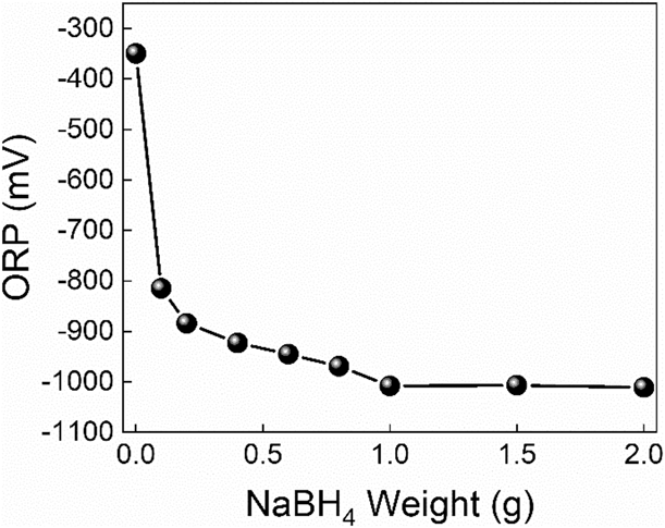
Figure 1 shows the ORP diagram of the reduction system with different NaBH4 dosages. The corresponding experimental samples were numbered as G-Sd-n (n = 1, 2, 3, …, 7, 8).
ORP diagram with different NaBH4 dosages. Eight different dosage values, from 0.1 to 2.0 g, were added into the reactor successively to determine the real-time ORPs of the corresponding system.

It can be seen from Fig. 1 that the initial ORP value of the system is −353 mV. Because the solvent is NaOH solution, it has a certain reduction effect on graphene oxide, and the ORP value decreases to a negative value after the reaction temperature is raised. With the increase of NaBH4 dosage, the ORP value of the system decreases gradually. When the NaBH4 dosage is more than 1.0 g, the ORP value of the system decreases to −1008.1 mV and tends to be stable, and the reductive properties of the system can no longer be improved by the addition of NaBH4. Therefore, the optimum initial dosage of NaBH4 is 1.0 g.
The reduction temperature and restore time
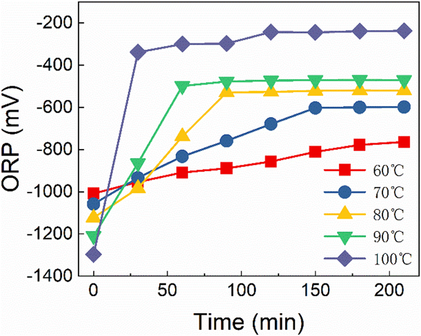
Figure 2 shows the variation of ORP value with different reduction temperature and time. In order to determine the best reduction temperature and time, the reduction temperatures of graphene oxide suspensions were set from 60 to 100 °C, at intervals of 10 °C. The corresponding experimental samples were numbered as G-St-n (n = 1, 2, 3, 4, 5).
ORP diagram with different reduction temperature and time. The mixture of graphene oxide and reductant reacted at different temperatures for a certain time, and the ORP value of the mixture was determined every 30 min.
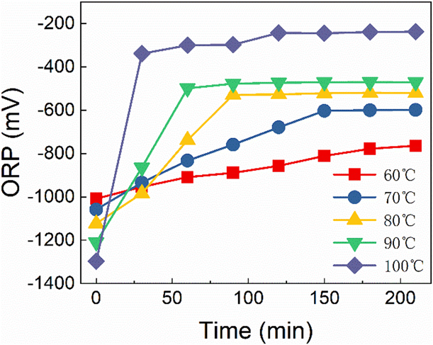
From the above Fig. 2, we can see that the initial ORP values of GS-2-n varies from −1303 to −1009 mV with the increase of temperature, and the initial value of G-St-5 at 100 °C is −1009 mV, while it is −1303 mV corresponding to G-St-1. The ORP values of G-St-n increases gradually as the reaction goes on, and the value of G-St-1 increases slowly all the time, which takes nearly 210 min to reach −810 mV, and then the reaction of other four samples reaches equilibriums after a period of time with the ORP remaining unchanged upon itself rising to a certain point.
Furthermore, we can find out the higher the temperature of G-St-n, the faster the equilibrium can be reached. It is for 30 min that the ORP of G-St-5 rises to −389 mV, while G-St-4 goes through 60 min to reach an equilibrium and the values of G-St-3 and G-St-2 remains unchanged after 90 min and 150 min with their final values are −557 mV and −611 mV, respectively.
Besides, we can find out that the greater the variation of the difference between the beginning and the end of ORP is, the higher the reduction degree of graphene oxide is. The ORP difference (∆ORP) of G-St-n samples is 199 mV, 440 mV, 575 mV, 695 mV, and 914 mV, respectively. However, when the reaction temperature is 100 °C, the volatilization of water in the solvent is much more serious, which leads to the increase of the concentration of reducing substances in the mixture, the ORP value increases correspondingly, and the reaction is violent and difficult to control. In other words, 100 °C is not suitable to be set as the reduction temperature. In addition, the ∆ORP of G-St-4, the maximum variation value, reaches 695 mV; therefore, it is appropriate to set 90 °C as the reaction temperature in the reduction process. In order to ensure the full reduction of graphene oxide, the reaction time would better be set to 210 min.
Effects of the redox potential on the productivity
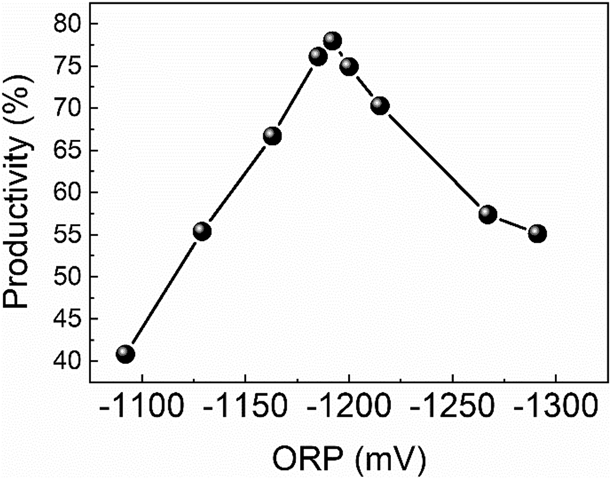
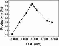
Figure 3 has shown the yield chart from a series of graphene products, G-SP-n (n = 1, 2, 3, …, 8, 9), prepared by different initial ORP values during the reduction phase of graphene oxide.
Graphene yield diagram prepared with different initial ORP values. The mass of graphite raw material from suspension was 2.0 g.

As can be seen from Fig. 3, graphene yields vary from 40 to 78%. With the decrease of the ORP value, the reduction ability of the system is enhanced, and the graphene yield increases at first and then decreases. The corresponding graphene yields of G-SP-4, G-SP-5, and G-SP-6 are 76.1%, 77%, and 74.9%, which are larger than that of other samples. Therefore, the optimal initial ORP interval in the reduction phase of graphene oxide is determined to be [−1200, −1180] mV [Reference He, Tian and Sun5, Reference Hu, Gao and Liu6].
Effects of the redox potential on the microscopic morphology
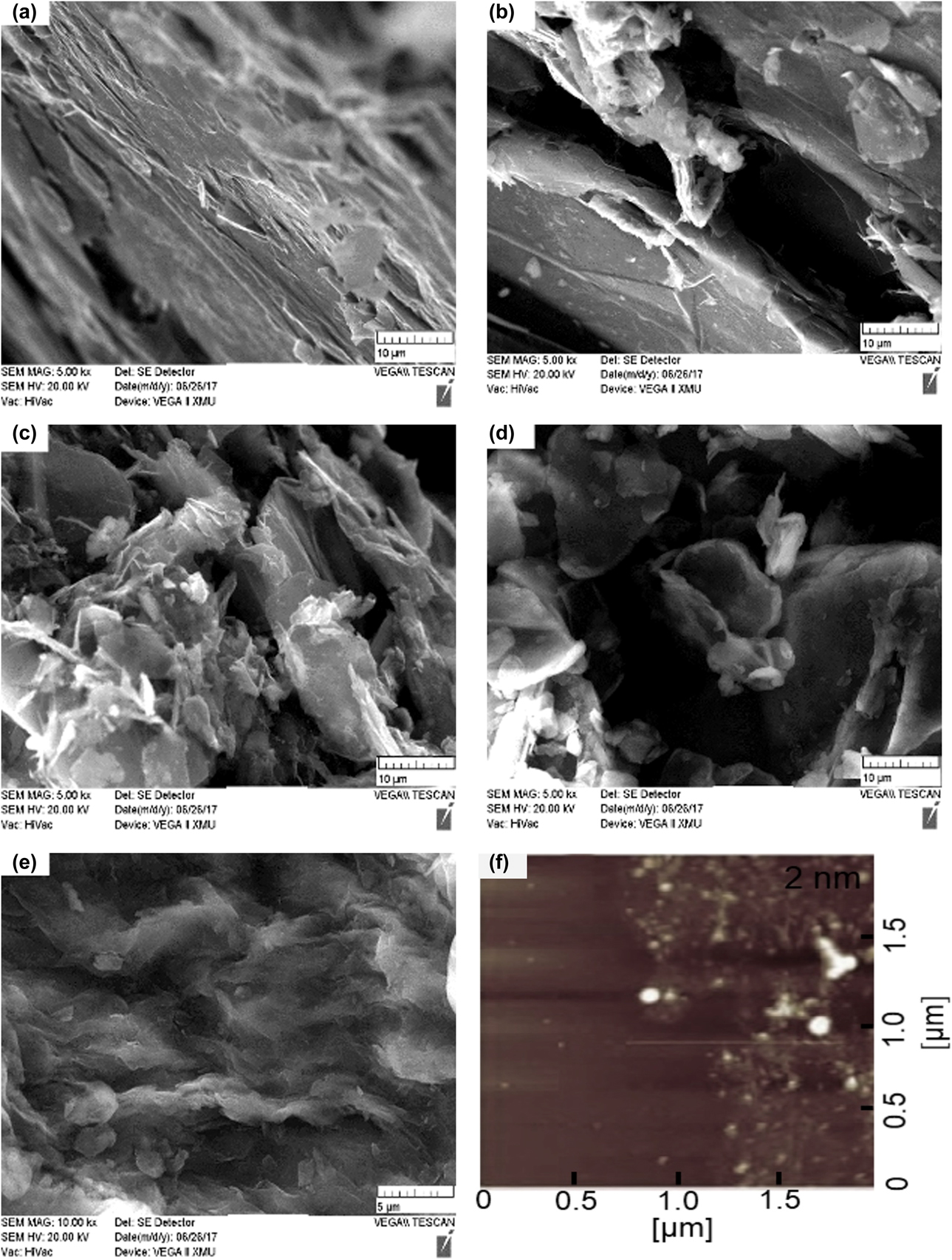
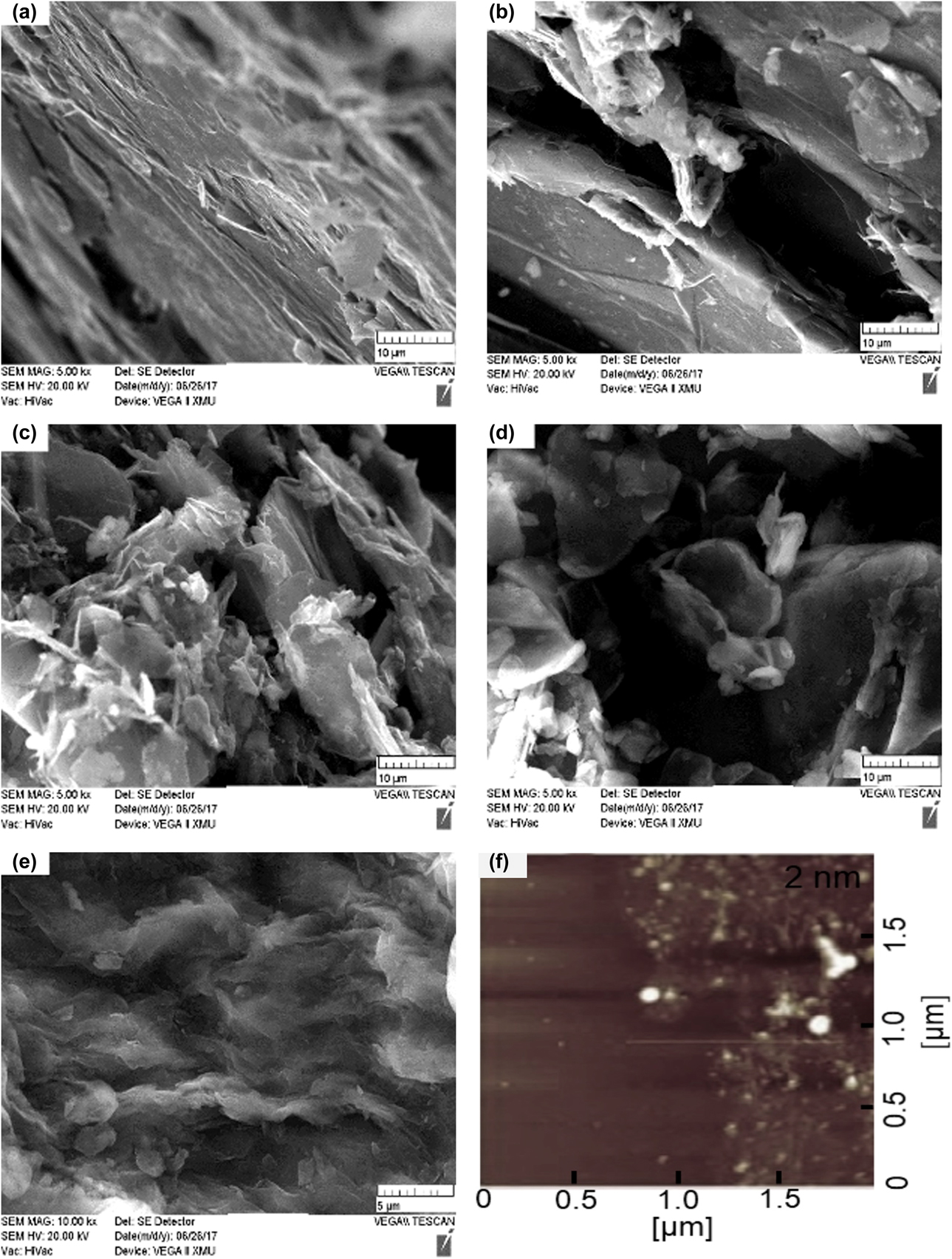
Figure 4 has shown a series of graphene products G-SS-n (n = 1, 2, 3, 4, 5), prepared by various initial ORP at the reduction stage and characterized by scanning electron microscope (SEM) and atomic force microscope (AFM). The result reveals that when the initial ORP of the reduction stage is relatively large and the amplification ratio is 5k times, the graphite structure layer is obviously layered and the surface is relatively smooth in the Figs. 4(a) and 4(b), which indicates that the graphite layer has not been exfoliated well. With the decrease of the ORP value, the layered structure of “graphite phase” gradually disappears, and there is almost no clearly visible layered structure and more folds in graphene form is present instead from Figs. 4(c) to 4(e). The closer the initial ORP value is to the optimal ORP interval, the more and more evenly distributed folds can be seen when observed at a high multiple of 20k times, which indicates that the graphite sheets are well peeled off to form homogeneous graphene. At the same time, combined with AFM characterization from Fig. 4(f), the thickness of G-SS-5 was approximately 2 nm. Considering the gap between the pattern and the substrate and the presence of functional groups, it can be calculated that its number of sheets is about 1 layer [Reference Chen, Jin and Liang7].
SEM and AFM diagrams of graphene products with different reduction degree. (a)–(e) refer to SEM image of G-SS-n (n = 1, 2, 3, 4, 5) and (f) refers to the AFM image of G-SS-5 and the thickness of its single layer is around 2 nm. Their initial ORPs are −1092 mV, −1129 mV, −1185 mV, −1192 mV, and −1200 mV, respectively.
Effects of the redox potential on the structural properties
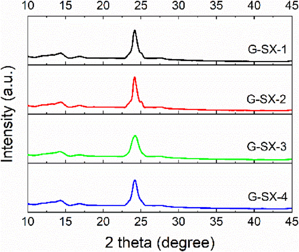
As shown in Fig. 5, it is X-ray diffraction (XRD) patterns of graphene products, G-SX-n (n = 1, 2, 3, 4). There are no obvious diffraction peaks in the XRD patterns of these products, and the characteristic diffraction peaks at 26.5° of graphite and 10° of graphite oxide have disappeared, but a new diffraction peak appears at 24°, with two weak diffraction peaks at 15°. This is mainly due to the stacking and aggregation of the reduced graphene lamellae after the graphite oxide structure layer is peeled off, so the peak value d 2θ at 24° could represent the distance between graphene stacking layers [Reference Chen, Jin and Liang7, Reference Sereshti, Khosraviani, Samadi and Amini-Fazl8]. Besides, the added fluorinated surfactant FC-4430 effectively reduced agglomeration. During the gradual reduction of graphene oxide, a locally ordered overlapping structure is formed, resulting in two weak second-order diffraction peaks around 15°.
XRD patterns of graphene products, G-SX-n (n = 1, 2, 3, 4), prepared by different initial ORPs: −1190 mV, −1210 mV, −1175 mV and −1180 mV, respectively.
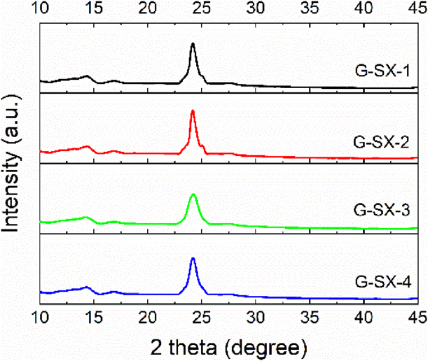
The microscopic size of graphene could be calculated according to Scherrer formula [Reference Gupta, Shaw and Saha9], that is,
 $${L_{\rm{c}}} = {{K\lambda } / {\beta \;\cos \;\theta }}\quad ,$$
where the value of Scherrer constant K is 0.89; the wavelength of XRD λ is 0.15406 nm; θ is the diffraction angle; β is the FWHM of the diffraction peak at the diffraction angle of 24°, which can be obtained by Gaussian fitting of the diffraction peak [Reference Andonovic, Temkov and Ademi10].
The stacking number of graphene can be obtained by dividing the size of microcrystals L c by the interlayer spacing of graphene d 2θ, i.e.,
 $$n = {{{L_{\rm{c}}}} / {{d_{2\theta }}}}\quad .$$
The obtained microcrystalline size L c and stacking number n of these products are calculated, among which the structure of G-SX-1 is a single-layer stacking layer, while other three products have multilevel layers, which indicates that the initial ORP value at the reduction stage is directly related to the final graphene quality, that is, the closer the initial ORP value is to the optimal ORP range, the smaller the stacking numbers of graphene products are [Reference Danilov, Slobodyanyuk and Rusetskii11, Reference Dervishi, Li, Watanabe, Biswas and Xu12].
Effects of the redox potential on the intrinsic properties
Raman spectroscopy has its unique advantages in characterizing graphene. Compared with other characterization techniques, Raman spectroscopy gives the intrinsic information of graphene and does not depend on the substrate used in characterization [Reference Cançado, Mateus, Martins Ferreira, Ferdinand, Katerina, Kai, Alain, Carlos, Rodrigo and Ado13].
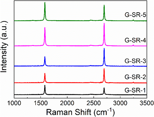
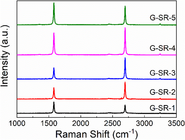
According to Fig. 6, there are two characteristic absorption peaks with G peak at 1579 cm−1 and 2D peak at 2696 cm−1, which are typical Raman peaks of graphene [Reference Budde, Cocalópez, Xian, Richard, Antonio, Duhee, Andrea and Achim14, Reference Beams, Gustavo and Novotny15, Reference Frolova, Magedov, Harper, Jha, Ovezmyradov, Chandler, Garacia, Donald, Shaner, Vasiliev and Kalugin16]. By integrating G peak and 2D peak and calculating their peak areas, we can find that the integral intensity ratios (I G/I 2D) of G-SR-n are 1.38, 0.76, 0.60, 0.91 and 1.29, respectively, among which strength ratio of G-SR-3 is 0.60, which reaches the minimum value. Combined with the optimal interval of initial ORPs, the initial potential of G-SR-3 is −1191 mV, from which we can draw a preliminary conclusion that the closer the initial ORP value is to the optimal ORP interval, the lower is the integral strength ratio of peak G divided by peak 2D.
Raman spectra of graphene products G-SR-n (n = 1, 2, 3, 4, 5) with two distinct characteristic peaks called G peak and 2D peak. The corresponding ORP values for these samples are −1138 mV, −1163 mV, −1191 mV, −1210 mV and −1297 mV, respectively.
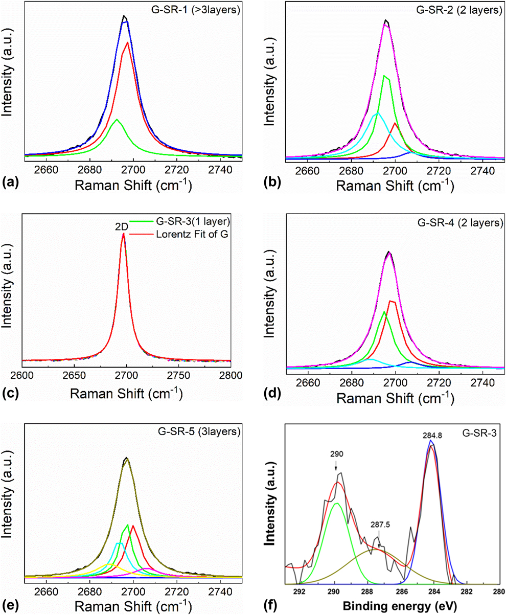
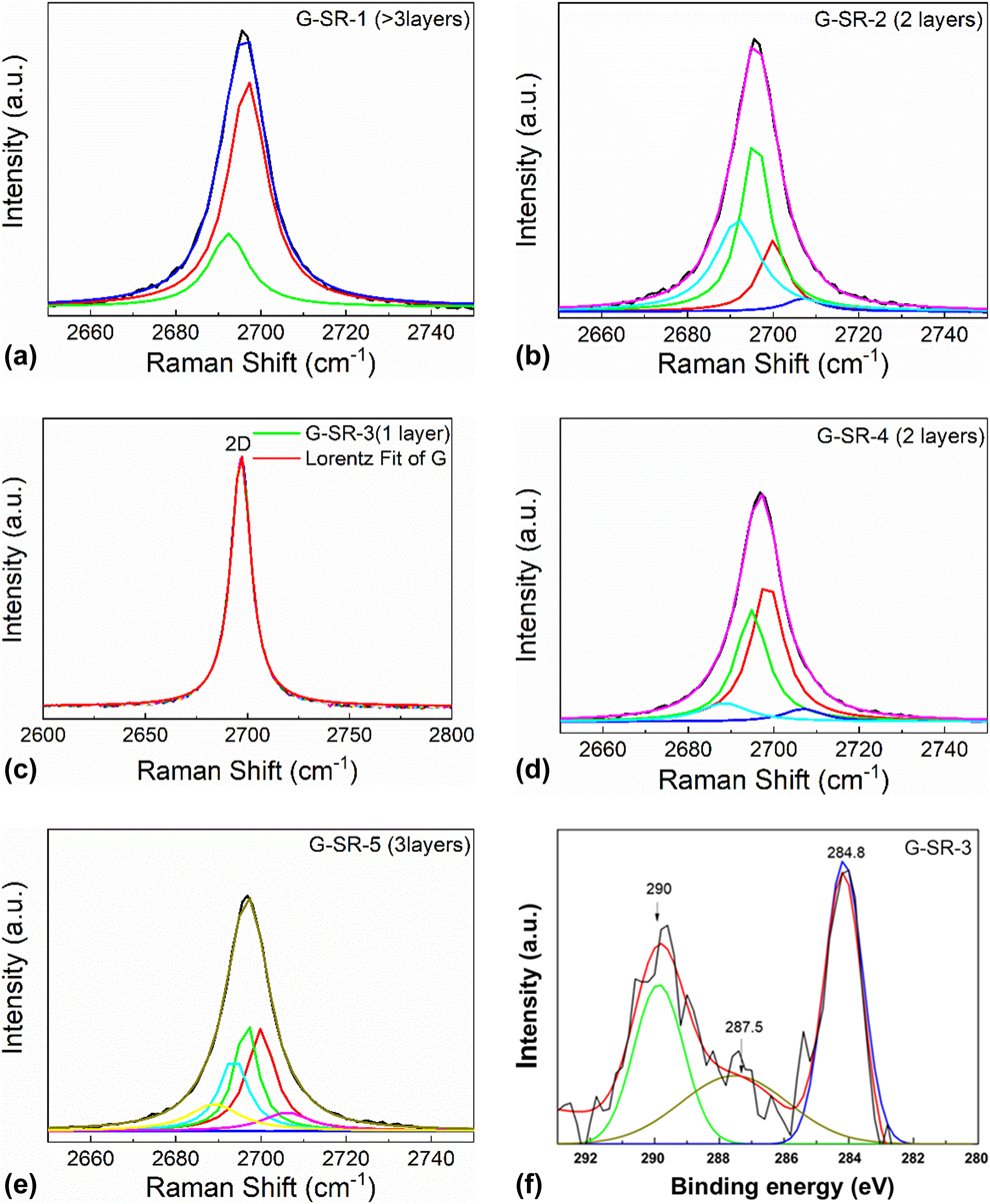
For the sake of further ascertaining the specific layers of graphene, the characteristic absorption peaks of products need Lorentz fitting and peak-splitting treatment. We mainly used Lorentz separation of 2D peak, because the shape and location of 2D peak and its relative strength with G peak were directly related to the number of graphene layers. Monolayer graphene can be used to synthesize a single Lorenz peak; double graphene can be fitted into four Lorenz peaks because of four possible double resonance scattering processes; similarly, three layers of graphene can be simulated to synthesize six Lorenz peaks. The double resonance scattering intensity increases with the increase of graphene layers. When graphene layers exceed 5 layers, it is difficult to distinguish the outline of Lorenz peak from graphite. Finally, there are only two Lorenz peaks just like graphite [Reference Ranjan, Tulika, Laha and Balakrishnan17].
Before Lorenz peak splitting, baseline adjustment and Lorenz fitting are needed for Raman spectra of the products. These products generally have three absorption peaks, G peak and 2D peak located in 1579.62 and 2696.72 cm−1, and 2G peak around 3200 cm−1. The baselines are adjusted first, and then the main absorption peaks are fitted by Lorenz. The G peak and 2D peak of graphene are synthesized to be independent peaks, which is convenient for obtaining various analysis parameters of Raman spectra, and is also conducive to the next step of Lorentz peak separation of 2D peaks. When the Raman 2D peak of the standard graphene sample purchased passes through the Lorentz fractionation to form a symmetrical Lorentz peak, it indicates that the number of layers is monolayer [Reference Budde, Cocalópez, Xian, Richard, Antonio, Duhee, Andrea and Achim14, Reference Cong and Yu18].
Figure 7 has illustrated that the 2D peak of G-SR-1 is divided into two Lorenz peaks, indicating that the number of layers is more than three layers. The 2D peak of G-SR-5 is divided into six Lorenz peaks, which reveals that the layers have three levels. The 2D peaks of G-SR-2 and G-SR-4 can be divided into four Lorenz peaks, which suggests that the figure for layers is two. G-SR-3 is intended to synthesize a highly symmetric Lorenz peak, which is similar to the fitting peak of the standard graphene sample, indicating that the graphene layer is the single layer. It is shown from above that the initial reduction ORP value of graphene preparation process is directly related to the layer number of graphene, which also determines the quality of graphene product. Because the initial ORP of G-SR-3 is within the optimal initial ORP range, its graphene yield is the highest among five products and the most ideal preparation effect as well. Combined with the peak-matching spectrum of its C 1s spectrum of XPS in Fig. 7(f), the C 1s spectrum can be mainly divided into three fitting peaks of 284.8, 287.5, and 290.0 eV. According to the standard C 1s spectral electronic energy spectrum table, the three fitted peaks correspond to characteristic peaks of C=C, C–O–C, and O–C=O, respectively [Reference Cong and Yu18]. With the optimization of the reduction potential of the reaction system, the characteristic absorption peak intensity of oxygen-containing energy groups like C–O–C and O–C=O would be gradually widening and weakening.
Lorenz splitting and fractionation for 2D peaks of G-SR-n (n = 1, 2, 3, 4, 5) and XPS diagram of G-SR-3. The black lines are the original peaks of 2D and their fitting peaks are expressed in different colors from (a)–(e) respectively. The fitting numbers indicate the figure for structural layers of graphene products; the black chromatogram line in (f) is the original XPS data of G-SR-3. After the peak fitting, three fitting peaks can be obtained with positions at 284.8, 287.5, and 290 eV.
It can be further determined that the integral strength ratio I G/I 2D has an inevitable relationship with graphene layer number [Reference Zhan, Olmedo, Wang and Liu19]. As I G/I 2D continues to grow, so does the number of layers. It is proved by many experiments that when I G/I 2D is less than 0.7, the graphene layer is monolayer; when I G/I 2D is between 0.7 and 1.0, it is double layer; and when I G/I 2D is between 1.0 and 1.3, it has three layers. However, when the ratio exceeds 1.3, there is no necessary relationship between the ratio and graphene layer number, because the higher the ratio is, the more obvious the “graphite phase structure” of the product will become [Reference Gayathri, Jayabal, Kottaisamy and Ramakrishnan20].
Conclusions
As is revealed by approaches of XRD, FT-IR, and Raman characterization, the optimum redox potential range, with HNO3–27S as the oxidant source of GO for preparing graphene, is from −1200 to −1185 mV. Within the optimum redox potential range, the yield of graphene, the target product, can be between 74.9 and 77.8%. As a result, a large amount of monolayer graphene can be formed with the conditions, under which the addition of reagents and the reaction temperature is precisely controlled. The research can be useful for simplifying preparation of graphene with chemical reduction, and also an important theoretical reference for the automation and industrialization in preparation of graphene.
Experimental methodology
Materials and apparatus
Natural flake graphite powder (NFG) (90 wt%, 50 mesh) was supplied by Qingdao Sheng-Ping Graphite Company (Qingdao, Shandong Province, China); KMnO4 (99.5 wt%), H2O2 (30.0 wt%), NaOH (96.0 wt%), NaBH4 (98.0 wt%) were bought from Xi’an Sanpu Chemical Reagent Co., Ltd. (Xi'an, Shannxi Province, China); HNO3–27S (HNO3 65.0 wt%, N2O4 25.0 wt%, HF 0.4 wt%, H3PO4 1.5 wt%), a common oxidizer for rocket liquid propellants, was obtained from Jilin Chemical Fertilizer Plant (Jilin, China); Fluorocarbon surfactant (FC-4430) was bought from American 3M Co., Ltd, (St. Paul, Minnesota).
X-ray diffraction (XRD) patterns were performed using a D8 ADVANCE system (Brook, Berlin, Germany) with Cu Kα radiation. Scanning electron microscope (SEM) observation was conducted by FEI Sirion Field Emission Gun SEM with energy dispersive X-ray spectroscopy (EDX) for the elemental analysis. The ORP determination was carried out with FJA-5 produced by Nanjing Chuandi instrument equipment Co., Ltd. (Nanjing, Jiangsu Province, China). Raman characterization was carried out using a RM-1000 Laser Confocal Raman Microspectroscopy (Renishaw, East Midlands, England) employing a 514.5 nm laser beam. Atomic force microscope (AFM) was from Bruker Fast Scan, Berlin, Germany; X-ray photoelectron spectroscopy (XPS: 40 kV, 40 mA) was from Bruker D8 Advance, Berlin, Germany.
Preparation of graphene
Two grams of graphite was added to the reaction kettle containing a certain amount of HNO3–27S, and then the kettle was placed in a constant temperature reaction bath below 5 °C, followed by the addition of 30 wt% H2O2 and 2 g FC-4430 with temperature unchanged; proper amount of KMnO4 was added slowly, the reaction kettle was moved into the heating sleeve, and the temperature was raised to keep the reaction for a certain period of time.
The above sample was stirred continuously, proper amount of ultrapure water was added, temperature was quickly raised and kept below 100 °C for 30 min, and then the sample was filtered immediately. The sample was washed with 5 wt% dilute hydrochloric acid and ultrapure water 5 times until it becomes neutral, filtered again, and dried at 60 °C for 12 h to obtain graphite oxide intermediate.
NaOH solution (pH = 11) was used as dispersant, the above sample was added into the reactor with 30-min ultrasonic dispersion and then high-speed centrifugation for 2 min. The sample was stirred mechanically and NaBH4 was added slowly, then stirring was continued and ORP determined at regular intervals until the ORP value remains stable for a period of time. The reduced graphene suspension was separated from the solid–liquid state, filtered, and dried at 100 °C for 6 h to obtain the target graphene product.
Productivity of graphene
After the above dried graphene was cooled to room temperature, it was weighed as m 1 by electronic balance and the mass of graphite raw material was recorded as m 2, then the yield of graphene could be calculated as follows:
 $$X = {m_1}/{m_2}\quad .$$
Competing interests
The authors declare that they have no competing interests.
Contributions
Both of the authors have taken part in the preparation of this manuscript, have reviewed the results, and have approved the final version of this manuscript. Prof. Wang conceived the idea and the experimental design of the project. Dr. Zhang performed all of the experiments and analyses.
Acknowledgments
The authors would like to thank Jilin Chemical Fertilizer Plant for financial support. The authors also thank Profs. X.X. Liu, Y.Z. Zhang and Dr. X.G. Mu for helpful discussions.