1 Introduction
The flow driven by a temperature difference imposed along a horizontal boundary is known as horizontal convection, which arises in myriad geophysical and industrial systems (Hughes & Griffiths Reference Hughes and Griffiths2008). A natural convection flow develops as a result of the horizontal temperature differences, which if sufficiently large lead to unsteady overturning circulation. Numerous studies (Mullarney, Griffiths & Hughes Reference Mullarney, Griffiths and Hughes2004; Sheard & King Reference Sheard and King2011; Gayen, Griffiths & Hughes Reference Gayen, Griffiths and Hughes2014) have focused on planar horizontal convection where the effects of thermal forcing and aspect ratio are investigated. However, this paper will focus on the effect of rotation on horizontal convection flows, which is important in many industrial applications as well as in geophysical flows, including circulations of ocean and atmospheres (Marshall & Schott Reference Marshall and Schott1999). More specifically, this paper addresses the linear stability of rotating horizontal convection to non-axisymmetric disturbances.
For non-rotating horizontal convection at high Rayleigh number, Rossby (Reference Rossby1965) demonstrated that the horizontal thermal layer has a thickness proportional to the
 $-1/5$
th power of Rayleigh number. However, in a rapidly rotating system, the thinnest horizontal boundary layer is the Ekman layer (Hignett, Ibbetson & Killworth Reference Hignett, Ibbetson and Killworth1981). The ratio between thermal boundary layer thickness and Ekman layer thickness is important in describing the flow; the square of this ratio (Park, & Whitehead Reference Park and Whitehead1999; Barkan, Winters & Smith Reference Barkan, Winters and Smith2013) is the non-dimensional rotation parameter
 $$\begin{eqnarray}Q=2\!\left(\frac{{\it\delta}_{{\it\theta}}}{d}\right)^{2},\end{eqnarray}$$
where the non-rotating thermal boundary layer thickness
 ${\it\delta}_{{\it\theta}}=R/\mathit{Ra}^{1/5}$
and
 $d=\sqrt{2{\it\nu}/f}$
is the Ekman depth.
 $R$
is the radius,
 $\mathit{Ra}$
is the horizontal Rayleigh number defined later in § 3,
 ${\it\nu}$
is the fluid kinematic viscosity and
 $f$
is the Coriolis frequency (
 $f=2{\it\Omega}$
, where
 ${\it\Omega}$
is the background rotation rate).
In a classical Rayleigh–Bénard convection, thermal buoyancy is the main source of instability production. On the other hand, the stability of rotating horizontal convection depends on the thermal gradient, vertical velocity shear as well as radial velocity shear. In fact, for rapidly rotating stratified fluids that are subjected to a horizontal temperature gradient, baroclinic instability originates as unstable wave-like disturbances (Lappa Reference Lappa2012). Charney (Reference Charney1947) and Eady (Reference Eady1949) developed a theoretical framework for the analysis of baroclinic instability in a rotating system, though in the practical confines of a laboratory apparatus, different types of instabilities can occur and might be hybrid in nature.
The important variables for baroclinic instability are the vertical shear of geostrophic velocities and the stratification. The Richardson number (
 $\mathit{Ri}$
) combines these two variables to characterise baroclinic instability in the ocean. Stone (Reference Stone1966, Reference Stone1970, Reference Stone1971) studied three-dimensional instability of baroclinic flow for small
 $\mathit{Ri}$
. They considered the Eady basic state of a plane baroclinic flow with constant temperature gradients and constant vertical shear. Horizontal shear was omitted, and viscous and thermal diffusion effects were neglected in both the basic state and perturbation analysis. They determined that conventional baroclinic instability dominates if
 $\mathit{Ri}>0.95$
, symmetric baroclinic instability dominates if
 $0.25\leqslant \mathit{Ri}\leqslant 0.95$
and Kelvin–Helmholtz instability dominates if
 $Ri<0.25$
. However, his results failed to predict the existence of symmetric baroclinic instability in the laboratory (Stone et al.
Reference Stone, Hess, Hadlock and Ray1969; Hadlock, Na & Stone Reference Hadlock, Na and Stone1972). Therefore, the studies on symmetric baroclinic instability which followed Stone’s analyses added viscous and thermal effects to make the model more representative.
The effects of rotation on horizontal convection have been investigated by Stern (Reference Stern1975), Hignett et al. (Reference Hignett, Ibbetson and Killworth1981), Barkan et al. (Reference Barkan, Winters and Smith2013) and more recently by Hussam, Tsai & Sheard (Reference Hussam, Tsai and Sheard2014). Hignett et al. (Reference Hignett, Ibbetson and Killworth1981) investigated the dynamics of horizontal convection in an annulus rotating about its central axis and a radial temperature gradient was maintained along the lower boundary. Their experiments focused on the rotating regime with
 $Q\sim O(1)$
. For a large Rayleigh number, six flow regimes were determined depending on the magnitude of parameter
 $Q$
. They found that for small
 $Q$
, the flow is only weakly modified by rotation, and the scaling laws for heat flux and thermal boundary layer thickness are similar to the non-rotating case (i.e. Rossby scaling for horizontal convection).
Experiments on thermal convection in annular geometry showed that when the rotation exceeds a certain critical value
 $Q_{c}\approx 3.4$
, Coriolis forces inhibit overturning motion in the meridional plane and promote a sloping convection or baroclinic waves flow. The sloping temperature surfaces can amplify a perturbation by converting potential energy into kinetic energy (Lappa Reference Lappa2012). Barkan et al. (Reference Barkan, Winters and Smith2013) performed a linear stability analysis on an analytical solution for rapidly rotating horizontal convection, and demonstrated that the sloping isopycnals (equivalent to isotherms in the present study) of the rotating horizontal convection flow result in greatly enhanced available potential energy, and hence the flow was expected to support baroclinic instability. The global stability of the flow within the enclosure remains an open question; one we address in the present study via a global linear stability analysis.
Barkan et al. (Reference Barkan, Winters and Smith2013) also performed direct numerical simulations of rotating horizontal convection in a rectangular enclosure with an arbitrary axis of rotation. They extended the previous studies by exploring the rapidly rotating
 $Q\gg 1$
regime (specifically up to
 $Q=24$
), which is more relevant to Earth’s oceans. They also discussed the effect of baroclinic eddies on the zonally averaged flows, as these are thought to play an important role in the dynamics of oceanic overturning circulation. Analysis extending the models of Smith (Reference Smith1976) and Whitehead (Reference Whitehead1981) applied to the rapidly rotating case did an excellent job of predicting the inclination of stratification in the interior. Their results demonstrated that rapid rotation and baroclinic instability significantly modify the steady state compared to non-rotating horizontal convection and therefore are essential components for the model of the overturning circulation and thermal structure of the ocean. They estimated a critical
 $Q_{c}=2.63$
for baroclinic instability based on a relation obtained by Hignett et al. (Reference Hignett, Ibbetson and Killworth1981) for the critical rotation parameter, and proceeded to compute baroclinically active rotating horizontal convection at a flux-based Rayleigh number
 $\mathit{Ra}_{B}=3.8\times 10^{9}$
and
 $Q=10$
. The present study seeks to obtain solutions at sufficiently high
 $Q$
to elucidate instabilities towards Hignett et al.’s very strong rotation regime.
Geophysical applications provoke interest in baroclinic instability in these flows, though in practice the finite enclosure of this system in laboratory set-ups inevitably render them susceptible to other instability mechanisms, including Stewartson layers arising from differential rotation between interior flow and sidewall shear layers (Stewartson Reference Stewartson1957; Hide & Titman Reference Hide and Titman1967; Früh & Read Reference Früh and Read1999; Vo, Montabone & Sheard Reference Vo, Montabone and Sheard2014, Reference Vo, Montabone and Sheard2015) and thermal instability in regions of strong adverse temperature gradient (Bodenschatz, Pesch & Ahlers Reference Bodenschatz, Pesch and Ahlers2000; King & Aurnou Reference King and Aurnou2012). A key question for the correct interpretation of laboratory investigations of baroclinically active flows and horizontally driven convection flows with rotation is therefore its global stability to axisymmetric and non-axisymmetric disturbances. The effects of eddies on large-scale flows are frequently predicted using residual mean theories (Andrews & McIntyre Reference Andrews and McIntyre1976, Reference Andrews and McIntyre1978) such as the transformed Eulerian-mean approach (Plumb & Ferrari Reference Plumb and Ferrari2005; Barkan et al. Reference Barkan, Winters and Smith2013). In the present study a global linear stability analysis is employed to predict the instability modes of the flow, and to interrogate the dominant instability modes using several approaches, including application of an energetics analysis of the azimuthally averaged perturbation fields to elucidate the dominant mechanisms of energy production and instability growth, and the change in potential energy density criterion to identify those modes with characteristics consistent with baroclinic instability (Lappa Reference Lappa2012; Barkan et al. Reference Barkan, Winters and Smith2013). A contribution of the present work is the spatial elucidation of the instability modes and their energetics.
The paper is organised as follows: § 2 briefly describes the system under investigation, § 3 introduces the governing equations, parameters, the change in potential energy criterion for baroclinic instability, the available potential energy, the linear stability analysis, the azimuthally averaged perturbation kinetic energy equation and the numerical code used herein. Section 4 contains the results of the axisymmetric computations, and § 5 contains results of the stability analysis and perturbation energy analysis. Finally, concluding remarks are presented in § 6.
2 System description
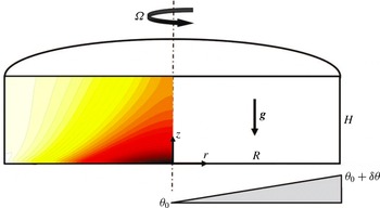
The system under consideration consists of a free-surface cylindrical enclosure rotating with an angular velocity
 ${\it\Omega}$
about its vertical axis of symmetry. It is filled with fluid, and a radially increasing temperature profile is imposed on the base. The tank radius
 $R$
and height
 $H$
combine to define an aspect ratio which in this study is fixed at
 $H/R=0.4$
. The system is depicted in figure 1.
Schematic representation of the system, showing key symbols. Representative contours of temperature are plotted on the computational domain spanning the meridional semi-plane.

Taking a velocity field in cylindrical coordinates,
 $\boldsymbol{u}(z,r,{\it\phi},t)=\langle u_{z},u_{r},u_{{\it\phi}}\rangle$
, the tank rotation is described by imposing an azimuthal velocity on the impermeable base and side wall as
 $u_{{\it\phi}}=r{\it\Omega}$
, where
 $r$
is the radial coordinate. To model a free surface, a stress-free condition is imposed on the top boundary (
 $u_{z}=\partial u_{r}/\partial z=\partial u_{{\it\phi}}/\partial z=0$
). The side wall is thermally insulated by imposition of a zero normal temperature gradient, and to simplify the computational model, no heat loss is permitted through the stress-free top surface, which is also approximated as being thermally insulated. A linear temperature profile with an increase of
 ${\it\delta}{\it\theta}$
from
 $r=0$
to
 $r=R$
along the base is imposed to drive horizontal convection in the
 $z$
–
 $r$
plane.
3 Numerical methodology
A Boussinesq approximation for fluid buoyancy is employed, in which density differences in the fluid are neglected except through the gravity term in the momentum equation (Barkan et al.
Reference Barkan, Winters and Smith2013). Under this approximation the thermodynamic equation reduces to a scalar advection–diffusion equation for temperature which is evolved in conjunction with the velocity field. The fluid temperature (
 ${\it\theta}$
) is related linearly to density (
 ${\it\rho}$
) via
 ${\it\rho}={\it\rho}_{0}[1-{\it\alpha}\left({\it\theta}-{\it\theta}_{0}\right)]$
, where
 ${\it\alpha}$
is the volumetric thermal expansion coefficient, while
 ${\it\theta}_{0}$
and
 ${\it\rho}_{0}$
are reference temperature and density, respectively.
The dimensionless incompressible Navier–Stokes equations and thermodynamic equation governing a Boussinesq fluid flowing in an inertial frame may be written as
 $$\begin{eqnarray}\boldsymbol{{\rm\nabla}}\boldsymbol{\cdot }\boldsymbol{u}=0,\end{eqnarray}$$
 $$\begin{eqnarray}\frac{\partial \boldsymbol{u}}{\partial t}=\boldsymbol{N}_{\boldsymbol{u}}-\boldsymbol{{\rm\nabla}}p+\frac{2}{Q\mathit{Ra}^{2/5}}{\rm\nabla}^{2}\boldsymbol{u}-\hat{\boldsymbol{g}}{\it\theta}\frac{4\mathit{Ra}^{1/5}}{\mathit{Pr}Q^{2}},\end{eqnarray}$$
 $$\begin{eqnarray}\frac{\partial {\it\theta}}{\partial t}=N_{{\it\theta}}+\frac{2}{\mathit{Pr}\,Q\mathit{Ra}^{2/5}}{\rm\nabla}^{2}{\it\theta},\end{eqnarray}$$
where nonlinear momentum and thermal advection terms are evaluated in convective form written as
 $\boldsymbol{N}_{\boldsymbol{u}}=-(\boldsymbol{u}\boldsymbol{\cdot }\boldsymbol{{\rm\nabla}})\boldsymbol{u}$
and
 $N_{{\it\theta}}=-(\boldsymbol{u}\boldsymbol{\cdot }\boldsymbol{{\rm\nabla}}){\it\theta}$
, respectively. Symbols
 $p$
,
 $t$
,
 $Q$
,
 $\mathit{Pr}$
and
 $\hat{\boldsymbol{g}}$
are the pressure, time, rotation parameter, Prandtl number and unit vector in the direction of gravity, respectively. In (3.1)–(3.3) and hereafter, lengths are scaled by
 $R$
, velocity by
 $R{\it\Omega}$
, time by
 ${\it\Omega}^{-1}$
, pressure by
 ${\it\rho}_{0}R^{2}{\it\Omega}^{2}$
(where
 ${\it\rho}_{0}$
is the reference density) and temperature by
 ${\it\delta}{\it\theta}$
.
A horizontal Rayleigh number characterising the thermal forcing is given by
 $$\begin{eqnarray}\mathit{Ra}=\frac{g{\it\alpha}\,{\it\delta}{\it\theta}R^{3}}{{\it\nu}{\it\kappa}_{T}},\end{eqnarray}$$
where
 $g$
is the gravitational acceleration and
 ${\it\kappa}_{T}$
is the thermal diffusivity of the fluid.
The rotation parameter (1.1) can be written
 $$\begin{eqnarray}Q=\frac{1}{\mathit{Ek}\,\mathit{Ra}^{2/5}}\left(\frac{H}{R}\right)^{-2},\end{eqnarray}$$
where
 $\mathit{Ek}$
is an Ekman number characterising the ratio of viscous to Coriolis forces (Hignett et al.
Reference Hignett, Ibbetson and Killworth1981)
 $$\begin{eqnarray}\mathit{Ek}=\frac{{\it\nu}}{2{\it\Omega}H^{2}}.\end{eqnarray}$$
The rotation parameter
 $Q$
accounts for the importance of rotation in horizontal convection. When
 $Q>O(1)$
, the thermal boundary layer is thicker and rotation is important. When
 $Q<O(1)$
, the Ekman boundary layer is thicker than the thermal boundary layer and frictional dissipation is important within the thermal boundary layer.
The Prandtl number of the fluid is given as
 $$\begin{eqnarray}\mathit{Pr}=\frac{{\it\nu}}{{\it\kappa}_{T}},\end{eqnarray}$$
and throughout this study
 $\mathit{Pr}=6.14$
, which approximates water at laboratory conditions. To explore the various modes of instability produced in a horizontal convection flow across the full span of rotation-affected flow regimes (Hussam et al.
Reference Hussam, Tsai and Sheard2014), a strongly convective Rayleigh number
 $\mathit{Ra}=10^{9}$
and rotation parameters (
 $0\leqslant Q\leqslant 60$
) are considered in the bulk of this study, while the Rayleigh number dependence of the stability is also considered. This range of rotation is below estimates of both molecular and turbulent values (
 $Q\approx 130$
and
 $210$
, respectively) for oceanic basin scale values on an
 $f$
-plane (Barkan et al.
Reference Barkan, Winters and Smith2013). However, the range both significantly exceeds the coverage of previous studies, and extends far beyond the estimated onset of baroclinic instability (
 $Q=O(1)$
).
3.1 Change in potential energy density
 ${\rm\Delta}\mathscr{E}_{p}$

In an inviscid flow with positive temperature gradients in both the upward vertical and horizontal directions, a particle moving from a colder higher region to a hotter lower region (while also traversing a horizontal distance
 ${\rm\Delta}L$
) experiences a change in potential energy density which under the Boussinesq approximation (Lappa Reference Lappa2012) is
 $$\begin{eqnarray}{\rm\Delta}\mathscr{E}_{p}=-g{\it\rho}_{0}{\it\alpha}\,{\rm\Delta}L^{2}{\it\xi}\frac{\partial {\it\theta}}{\partial r}\left[1-\frac{{\it\xi}}{{\it\delta}}\right],\end{eqnarray}$$
where
 ${\it\xi}$
is the angle from the horizontal of the path taken by the particle, and
 ${\it\delta}=\tan ^{-1}(-\partial _{r}{\it\theta}/\partial _{z}{\it\theta})$
is the inclination of the lines of constant temperature to the horizontal. When
 $0<{\it\xi}<{\it\delta}$
,
 ${\rm\Delta}\mathscr{E}_{p}<0$
and potential energy is released, which may amplify a perturbation by converting potential energy to kinetic energy, leading to baroclinic instability. Differentiating with respect to
 ${\it\xi}$
demonstrates that the maximum energy transfer occurs when
 ${\it\xi}={\it\delta}/2$
. This optimal orientation relates the horizontal displacement to a fixed particle path length through
 ${\rm\Delta}L=L_{p}\cos ({\it\delta}/2)$
, and hence equation (3.8) can be expressed for change in potential energy normalised by path length squared as
 $$\begin{eqnarray}\frac{{\rm\Delta}\mathscr{E}_{p}}{{L_{p}}^{2}}=-\frac{1}{4}\mathit{Ra}\,{\it\delta}\cos ^{2}\left(\frac{{\it\delta}}{2}\right)\!\frac{\partial {\it\theta}}{\partial r},\end{eqnarray}$$
where
 ${\rm\Delta}\mathscr{E}_{p}/{L_{p}}^{2}$
is normalised by
 ${\it\rho}_{0}{\it\nu}{\it\kappa}/R^{4}$
. Equation (3.9) will be plotted on axisymmetric base flow fields to identify those regions where the necessary condition for baroclinic instability,
 ${\rm\Delta}\mathscr{E}_{p}<0$
, is satisfied. Interpretation of modes will be aided by considering the alignment of disturbance mode structures with regions of negative
 ${\rm\Delta}\mathscr{E}_{p}$
, while instability structures confined to regions of
 ${\rm\Delta}\mathscr{E}_{p}>0$
would suggest a non-baroclinic origin. As a necessary but not sufficient criterion for baroclinic instability, (3.9) may yield
 ${\rm\Delta}\mathscr{E}_{p}<0$
in flows where baroclinic instability is not observed, and its inviscid and local nature may lead to disparity against the global stability solutions for the viscous flows obtained within this study. A powerful alternative for assessing the capacity for a flow to be baroclinically active is the available potential energy (Winters & Barkan Reference Winters and Barkan2013), which is described in the subsection to follow.
3.2 Available potential energy
$E_{a}$
and density
$\mathscr{E}_{a}$


The development of baroclinic instability is contingent on potential energy in the fluid being available for conversion to kinetic energy. The elaboration to follow draws from Winters et al. (Reference Winters, Lombard, Riley and D’Asaro1995), Winters & Barkan (Reference Winters and Barkan2013) and references therein, and in this subsection quantities are expressed in their dimensional form. To begin, at any instant in time a body of fluid contains a total potential energy
 $$\begin{eqnarray}E_{p}\equiv g\int {\it\rho}z\,\text{d}\mathscr{V},\end{eqnarray}$$
where
 $\mathscr{V}$
is the fluid volume. If we imagine permitting the parcels of fluid to adiabatically (i.e. without heat or molecular mass transfer Winters et al.
Reference Winters, Lombard, Riley and D’Asaro1995) settle to their equilibrium heights, then a minimum potential energy state is achieved, known as the background potential energy
 $E_{b}\equiv g\int {\it\rho}z_{\ast }\,\text{d}\mathscr{V}$
. Here
 $z_{\ast }(\boldsymbol{x},t)$
is the equilibrium height of fluid parcel with density
 ${\it\rho}$
, and the one-dimensional function
 ${\it\rho}(z_{\ast })$
is independent of the spatial distribution of fluid parcels.
It follows then that the available potential energy is the difference between potential and background potential energies, i.e.
 $$\begin{eqnarray}E_{a}=E_{p}-E_{b}=g\int {\it\rho}(z-z_{\ast })\,\text{d}\mathscr{V}.\end{eqnarray}$$
Winters & Barkan (Reference Winters and Barkan2013) made the further contribution of defining the available potential energy density
 $\mathscr{E}_{a}(\boldsymbol{x},t)$
, a positive-definite field that integrates to the total available potential energy, i.e.
 $$\begin{eqnarray}E_{a}=g\int \mathscr{E}_{a}\,\text{d}\mathscr{V}.\end{eqnarray}$$
The available potential energy density is zero where fluid parcels are at their equilibrium height, and larger values indicate greater displacement from equilibrium. It is formally defined as
 $$\begin{eqnarray}\displaystyle & \displaystyle \mathscr{E}_{a}\equiv \left(z-z_{\ast }\right)\left[{\it\rho}(\boldsymbol{x},t)-\bar{{\it\rho}}(z,z_{\ast })\right], & \displaystyle\end{eqnarray}$$
 $$\begin{eqnarray}\displaystyle & \displaystyle \bar{{\it\rho}}(z,z_{\ast })={\displaystyle \frac{1}{z-z_{\ast }}}\int _{z_{\ast }}^{z}{\it\rho}(z_{\ast }^{\prime })\,\text{d}z_{\ast }^{\prime }. & \displaystyle\end{eqnarray}$$
For convenience (3.13)–(3.14) are recast in terms of temperature consistent with (3.1)–(3.3), yielding
 $$\begin{eqnarray}\mathscr{E}_{a}\equiv {\it\alpha}{\it\rho}_{0}\left[\int _{z_{\ast }}^{z}{\it\theta}(z_{\ast }^{\prime })\,\text{d}z_{\ast }^{\prime }-\left(z-z_{\ast }\right){\it\theta}(\boldsymbol{x},t)\right].\end{eqnarray}$$
When presented in this study,
 $\mathscr{E}_{a}$
is given in dimensionless form, scaled by
 ${\it\rho}_{0}{\it\nu}{\it\kappa}/gR^{2}$
.
Winters & Young (Reference Winters and Young2009), Winters & Barkan (Reference Winters and Barkan2013) describe horizontal convection as being driven by the conversion of available potential energy to kinetic energy, emphasising the importance of the
 $\mathscr{E}_{a}$
distribution and buoyancy fluxes in these flows. Buoyancy relates to temperature through a linear equation of state approximation,
 $b={\it\alpha}g{\it\theta}$
.
3.3 Linear stability analysis
The potential for non-axisymmetric three-dimensional instability developing and significantly altering its characteristics on an axisymmetric base flow motivates an application of linear stability analysis. In this analysis, first an axisymmetric solution to equations (3.1)–(3.3) is obtained by fixing
 $\partial /\partial {\it\phi}=0$
. Then the linearised governing equations are obtained by decomposing the velocity, pressure and temperature into the sum of an axisymmetric field (
 $\bar{\boldsymbol{u}}$
,
 $\bar{p}$
,
 $\bar{{\it\theta}}$
) and a small non-axisymmetric perturbation (
 $\boldsymbol{u}^{\prime }$
,
 $p^{\prime }$
,
 ${\it\theta}^{\prime }$
). The perturbation field is constructed as a single complex Fourier mode of an azimuthal expansion of the flow field and the wavenumber of the perturbation is a parameter in the stability analysis. Substituting these into (3.1)–(3.3) and retaining only terms of order of the perturbation field yields the linearised Navier–Stokesand thermodynamic equations
 $$\begin{eqnarray}\boldsymbol{{\rm\nabla}}\boldsymbol{\cdot }\boldsymbol{u}^{\prime }=0,\end{eqnarray}$$
 $$\begin{eqnarray}\frac{\partial \boldsymbol{u}^{\prime }}{\partial t}=\boldsymbol{L}_{\boldsymbol{u}}^{\prime }-\boldsymbol{{\rm\nabla}}p^{\prime }+\frac{2}{Q\mathit{Ra}^{2/5}}{\rm\nabla}^{2}\boldsymbol{u}^{\prime }-\hat{\boldsymbol{g}}{\it\theta}^{\prime }\frac{4\mathit{Ra}^{1/5}}{\mathit{Pr}Q^{2}},\end{eqnarray}$$
 $$\begin{eqnarray}\frac{\partial {\it\theta}^{\prime }}{\partial t}=L_{{\it\theta}}^{\prime }+\frac{2}{\mathit{Pr}\,Q\mathit{Ra}^{2/5}}{\rm\nabla}^{2}{\it\theta}^{\prime },\end{eqnarray}$$
where the linear advection terms are
 $\boldsymbol{L}_{\boldsymbol{u}}^{\prime }=-[(\bar{\boldsymbol{u}}\boldsymbol{\cdot }\boldsymbol{{\rm\nabla}})\boldsymbol{u}^{\prime }+(\boldsymbol{u}^{\prime }\boldsymbol{\cdot }\boldsymbol{{\rm\nabla}})\bar{\boldsymbol{u}}]$
and
 $L_{{\it\theta}}^{\prime }=-[(\bar{\boldsymbol{u}}\boldsymbol{\cdot }\boldsymbol{{\rm\nabla}}){\it\theta}^{\prime }+(\boldsymbol{u}^{\prime }\boldsymbol{\cdot }\boldsymbol{{\rm\nabla}})\bar{{\it\theta}}]$
.
An operator
 $\mathscr{A}(T)$
is defined as being equivalent to time integration of a perturbation field by equations (3.16–3.18) over some time interval
 $T$
. Linear stability of a base flow of a given
 $(\mathit{Ra},Q,\mathit{Pr})$
and azimuthal wavenumber
 ${\it\beta}$
is dictated by the leading eigenmode of
 $\mathscr{A}(T)$
, which is obtained using an implicitly restarted Arnoldi method in conjunction with time integration of the base flow and one or more perturbation fields (Cogan, Ryan & Sheard Reference Cogan, Ryan and Sheard2011; Vo et al.
Reference Vo, Montabone and Sheard2015). The leading complex eigenvalue
 $|{\it\mu}|$
is related to the exponential growth rate
 ${\it\sigma}$
of the corresponding eigenmode (corresponding to the most asymptotically unstable perturbation field) via
 ${\it\sigma}=\log |{\it\mu}|/T$
. In the case of steady-state base flows (all cases considered in this study reach a steady-state axisymmetric equilibrium),
 $T$
may be chosen arbitrarily. If
 $|{\it\mu}|>1$
for any
 ${\it\beta}$
, then
 ${\it\sigma}>0$
and the flow is unstable, whereas if
 $|{\it\mu}|<1$
for all
 ${\it\beta}$
, then the axisymmetric flow is asymptotically stable to all infinitesimal disturbances. The azimuthal wavenumber relates to the azimuthal wavelength of the instability through
 ${\it\beta}=2{\rm\pi}/{\it\lambda}$
.
3.4 Azimuthally averaged perturbation kinetic energy
To complement the linear stability analysis, consideration is given to energy conversion from the base flow to growing disturbances via analysis of the volume integrated energetics of the predicted eigenmodes (Gill Reference Gill1982; Ménesguen, McWilliams & Molemaker Reference Ménesguen, McWilliams and Molemaker2012). The fluctuation kinetic energy per unit mass is defined as
 $k^{\,\prime }=({u_{z}^{\prime }}^{2}+{u_{r}^{\prime }}^{2}+{u_{{\it\phi}}^{\prime }}^{2})/2$
, and an equation describing its evolution is obtained by taking the dot product of
 $\boldsymbol{u}^{\prime }$
with (3.17), given that
 $\partial _{t}k^{\,\prime }=(1/2)\partial _{t}(\boldsymbol{u}^{\prime }\boldsymbol{\cdot }\boldsymbol{u}^{\prime })=\boldsymbol{u}^{\prime }\boldsymbol{\cdot }\partial _{t}\boldsymbol{u}^{\prime }$
. The azimuthal average of the equation is then taken (denoted by overbars), resulting in the azimuthally averaged perturbation kinetic energy equation
 $$\begin{eqnarray}\displaystyle \frac{\partial \overline{k^{\,\prime }}}{\partial t} & = & \displaystyle -\left[\bar{u}_{z}\frac{\partial \overline{k^{\,\prime }}}{\partial z}+\bar{u}_{r}\frac{\partial \overline{k^{\,\prime }}}{\partial r}\right]+\{\text{Divergence terms}\}\nonumber\\ \displaystyle & & \displaystyle -\,\left[\overline{{u_{z}^{\prime }}^{2}}\frac{\partial \bar{u}_{z}}{\partial z}+\overline{u_{z}^{\prime }u_{r}^{\prime }}\frac{\partial \bar{u}_{z}}{\partial r}+\overline{u_{r}^{\prime }u_{z}^{\prime }}\frac{\partial \bar{u}_{r}}{\partial z}+\overline{{u_{r}^{\prime }}^{2}}\frac{\partial \bar{u}_{r}}{\partial r}+\overline{u_{{\it\phi}}^{\prime }u_{z}^{\prime }}\frac{\partial \bar{u}_{{\it\phi}}}{\partial z}+\overline{u_{{\it\phi}}^{\prime }u_{r}^{\prime }}\frac{\partial \bar{u}_{{\it\phi}}}{\partial r}\right.\nonumber\\ \displaystyle & & \displaystyle \left.-\,\overline{u_{{\it\phi}}^{\prime }u_{r}^{\prime }}\frac{\bar{u}_{{\it\phi}}}{r}+\overline{{u_{{\it\phi}}^{\prime }}^{2}}\frac{\bar{u}_{r}}{r}\right]-\frac{4}{Q\,\mathit{Ra}^{2/5}}\;\overline{\unicode[STIX]{x1D634}_{ij}^{\,\prime }\unicode[STIX]{x1D634}_{ij}^{\,\prime }}+\frac{4\mathit{Ra}^{1/5}}{\mathit{Pr}\,Q^{2}}\;\overline{u_{z}^{\prime }{\it\theta}^{\prime }},\end{eqnarray}$$
where
 $$\begin{eqnarray}\overline{k^{\,\prime }}={\textstyle \frac{1}{2}}\left(\overline{u_{z}^{\prime }u_{z}^{\prime }}+\overline{u_{r}^{\prime }u_{r}^{\prime }}+\overline{u_{{\it\phi}}^{\prime }u_{{\it\phi}}^{\prime }}\right)\end{eqnarray}$$
and
 $\unicode[STIX]{x1D634}_{ij}^{\,\prime }$
is the instantaneous rate-of-strain tensor, which in cylindrical (
 $z$
,
 $r$
,
 ${\it\phi}$
) coordinates is written
 $$\begin{eqnarray}\unicode[STIX]{x1D634}_{ij}^{\,\prime }={\displaystyle \frac{1}{2}}\left[\begin{array}{@{}ccc@{}}2{\displaystyle \frac{\partial u_{z}^{\prime }}{\partial z}} & {\displaystyle \frac{\partial u_{z}^{\prime }}{\partial r}}+{\displaystyle \frac{\partial u_{r}^{\prime }}{\partial z}} & {\displaystyle \frac{\partial u_{{\it\phi}}^{\prime }}{\partial z}}+{\displaystyle \frac{1}{r}}{\displaystyle \frac{\partial u_{z}^{\prime }}{\partial {\it\phi}}}\\ {\displaystyle \frac{\partial u_{z}^{\prime }}{\partial r}}+{\displaystyle \frac{\partial u_{r}^{\prime }}{\partial z}} & 2{\displaystyle \frac{\partial u_{r}^{\prime }}{\partial r}} & r{\displaystyle \frac{\partial }{\partial r}}\!\left({\displaystyle \frac{u_{{\it\phi}}^{\prime }}{r}}\right)+{\displaystyle \frac{1}{r}}{\displaystyle \frac{\partial u_{r}^{\prime }}{\partial {\it\phi}}}\\ {\displaystyle \frac{\partial u_{{\it\phi}}^{\prime }}{\partial z}}+{\displaystyle \frac{1}{r}}{\displaystyle \frac{\partial u_{z}^{\prime }}{\partial {\it\phi}}} & r{\displaystyle \frac{\partial }{\partial r}}\!\left({\displaystyle \frac{u_{{\it\phi}}^{\prime }}{r}}\right)+{\displaystyle \frac{1}{r}}{\displaystyle \frac{\partial u_{r}^{\prime }}{\partial {\it\phi}}} & {\displaystyle \frac{2}{r}}\!\left({\displaystyle \frac{\partial u_{{\it\phi}}^{\prime }}{\partial {\it\phi}}}+u_{r}^{\prime }\right).\end{array}\right].\end{eqnarray}$$
For brevity we have adopted tensor notation to represent the double-dot-product of the rate-of-strain tensor (i.e.
 $\unicode[STIX]{x1D634}_{ij}^{\,\prime }\unicode[STIX]{x1D634}_{ij}^{\,\prime }$
represents the sum of the square of each element in
 $\unicode[STIX]{x1D634}_{ij}^{\,\prime }$
).
In (3.19), the left-hand side is the rate of change of azimuthally averaged perturbation kinetic energy due to time dependence in the perturbation field, and the first group of terms (in square brackets) on the right-hand side describes the rate of change of azimuthally averaged perturbation kinetic energy due to its advection on the base flow in the
 $r$
–
 ${\it\phi}$
plane. Omitted from the right-hand side are the divergence terms, which describe transport of azimuthally averaged kinetic energy on the
 $r$
–
 ${\it\phi}$
plane due to pressure fluctuations and viscous stresses, but which identically contribute nothing to the overall change in the integral of
 $\overline{k^{\,\prime }}$
over the flow domain. The next group of terms on the right-hand side describe the rate of
 $\overline{k^{\,\prime }}$
production from shear in the base flow. Following this is a term describing the rate of
 $\overline{k^{\,\prime }}$
dissipation due to viscous stresses, and finally a perturbation buoyancy flux term. In general, this last term would be written
 $-(4\mathit{Ra}^{1/5}/\mathit{Pr}\,Q^{2})[{\hat{g}}_{r}\overline{u_{r}^{\prime }{\it\theta}^{\prime }}+{\hat{g}}_{{\it\phi}}\overline{u_{{\it\phi}}^{\prime }{\it\theta}^{\prime }}+{\hat{g}}_{z}\overline{u_{z}^{\prime }{\it\theta}^{\prime }}]$
, with
 ${\hat{g}}_{z}$
,
 ${\hat{g}}_{r}$
and
 ${\hat{g}}_{{\it\phi}}$
being components of the unit vector in the direction of gravity, but in (3.19) only the axial component is included as gravity acts solely in the negative axial (downward) direction in the present study.
The perturbation buoyancy flux describes the reversible exchange of energy between potential energy in the axisymmetric base flow and kinetic energy in the perturbation field. This may be demonstrated by considering the evolution of potential energy. Winters et al. (Reference Winters, Lombard, Riley and D’Asaro1995) combine their buoyancy transport equation and the incompressibility constraint to obtain an evolution equation for total potential energy; here instead the local potential energy evolution is considered. Defining a potential energy density
 $\mathscr{E}_{p}={\it\rho}z$
such that (3.10) becomes
 $E_{p}\equiv g\int \mathscr{E}_{p}\,\text{d}\mathscr{V}$
, which has axisymmetric mean and fluctuating perturbation components
 $\bar{\mathscr{E}}_{p}$
and
 $\mathscr{E}_{p}^{\prime }$
, respectively, appendix A details the derivation of the evolution equation for azimuthally averaged potential energy density in the mean flow. In dimensionless form this equation is written
 $$\begin{eqnarray}{\displaystyle \frac{\partial \bar{\mathscr{E}_{p}}}{\partial t}}=-(\bar{\boldsymbol{u}}\boldsymbol{\cdot }\boldsymbol{{\rm\nabla}})\bar{\mathscr{E}}_{p}-\overline{(\boldsymbol{u}^{\prime }\boldsymbol{\cdot }\boldsymbol{{\rm\nabla}})\mathscr{E}_{p}^{\prime }}-\frac{4\mathit{Ra}^{1/5}\mathit{Fr}}{\mathit{Pr}Q^{2}}\left[\bar{u}_{z}\bar{{\it\theta}}+\overline{u_{z}^{\prime }{\it\theta}^{\prime }}\right]+\frac{2}{\mathit{Pr}Q\mathit{Ra}^{2/5}}z{\rm\nabla}^{2}\bar{{\it\rho}},\end{eqnarray}$$
where a Froude number
 $\mathit{Fr}=R{\it\Omega}^{2}/g$
has been introduced. The first two terms on the right-hand side of (3.22) describe advective transport of potential energy density by the mean flow and perturbation, respectively. The third term describes vertical advective buoyancy fluxes in the mean flow and perturbation field and the final term describes the effect of thermal dissipation in the mean flow. When comparing the prefactors to the dimensionless azimuthally averaged vertical advective buoyancy flux terms in the perturbation kinetic energy equation (3.19) and (3.22), the Froude number captures the ratio of the quantities used to scale kinetic and potential energy in the present study. Notice that in (3.22) the perturbation buoyancy flux term is negative, whereas the corresponding term is positive in (3.19), reflecting the reversible exchange role of these terms. Crucially, vertical advective buoyancy flux facilitates a conversion of potential energy in the axisymmetric mean flow to kinetic energy in a non-axisymmetric perturbation.
The power of equation (3.19) is revealed when we consider its application to the predicted linear instability modes of the axisymmetric base flows. These modes necessarily exhibit exponential growth (at a rate
 ${\it\sigma}$
), and it is straightforward to show then that
 $$\begin{eqnarray}{\it\sigma}=\frac{1}{2E_{k}}\int _{\mathscr{V}}\frac{\partial \overline{k^{\,\prime }}}{\partial t}\,\text{d}\mathscr{V},\end{eqnarray}$$
where total perturbation kinetic energy
 $E_{k}=\int _{{\it\Omega}}\overline{k^{\,\prime }}\,\text{d}\mathscr{V}$
. Hence when normalised by
 $2E_{k}$
, (3.19) equates to the exponential growth rate of eigenmodes arising from the linear stability analysis, and therefore, the integrals of each term normalised by
 $2E_{k}$
provide insight into their individual contributions to the overall growth or decay of each instability mode. Furthermore, the spatial variation of each term on the
 $z$
–
 $r$
plane will provide insight into the local features of the underlying axisymmetric velocity and temperature fields that most actively contribute to the instability growth, facilitating a quantitative basis for the classification of instability modes reported herein.
3.5 Spatial and temporal discretisation
The governing equations (3.1)–(3.3) are solved in cylindrical coordinates using a nodal spectral element method in space, and a third-order scheme based on backwards differentiation is employed for time integration (Karniadakis, Israeli & Orszag Reference Karniadakis, Israeli and Orszag1991). The same scheme is also employed for solution of the linearised equations (3.16)–(3.18). Lagrangian tensor-product polynomial shape functions are imposed upon each macro-element. The polynomial order is varied to control spatial resolution and interpolated at the Gauss–Lobatto–Legendre quadrature points. The cylindrical formulation of the solver employed here has been validated in previous studies (Sheard & Ryan Reference Sheard and Ryan2007; Sheard Reference Sheard2009) and was used recently to study axisymmetric rotating radial horizontal convection by Hussam et al. (Reference Hussam, Tsai and Sheard2014).
The computational domain in the
 $z$
–
 $r$
plane is discretised into quadrilateral elements. A rectangular mesh comprising
 $1320$
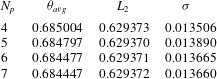
elements was constructed to discretise the meridional semi-plane. To resolve the flow accurately, the grid size was much smaller in the vicinity of the side and bottom walls, particularly the heated boundary, with coarser grid spacing in the interior. A grid resolution study was undertaken to determine a suitably accurate element polynomial degree. The test was performed at the upper end of the parameter range of this study,
 $\mathit{Ra}=10^{9}$
and
 $Q=60$
as a stringent test of the mesh resolution. Three parameters are monitored for convergence: domain integral of temperature (
 ${\it\theta}_{avg}$
) and square of velocity magnitude (
 $L_{2}$
), and the growth rate of the leading eigenmode obtained from the linear stability analysis at the dominant azimuthal wavenumber (
 ${\it\sigma}$
). As shown in table 1,
 ${\it\theta}_{avg}$
and
 $L_{2}$
are highly resolved:
 ${\it\theta}_{avg}$
errors between polynomial degree
 $N_{p}$
and
 $N_{p}+1$
decrease from
 $3.0\times 10^{-2}\,\%$
down to
 $4.4\times 10^{-3}\,\%$
from
 $N_{p}=4$
to
 $6$
, while
 $L_{2}$
errors decrease from
 $4.8\times 10^{-4}\,\%$
down to
 $1.6\times 10^{-4}\,\%$
. However, the higher resolution required to resolve the instability eigenmodes is reflected in the
 ${\it\sigma}$
case, with errors decreasing from
 $2.8\,\%$
at
 $N_{p}=4$
down to
 $3.7\times 10^{-2}\,\%$
. Hence
 $N_{p}=7$
is used hereafter to constrain errors to less than
 $O(0.1\,\%)$
.
For time integration of equations (3.2)–(3.3), the advection/convection terms are concurrently solved explicitly, followed by a projection of the velocity field onto a divergence-free space, and finally implicit solves for velocity components and temperature. This procedure extends the backwards differentiation algorithm of Karniadakis et al. (Reference Karniadakis, Israeli and Orszag1991) to the coupled Boussinesq equations. The temperature transport formulation of the present code has been validated in studies on buoyancy-driven flows (Sheard & King Reference Sheard and King2011; Hussam et al. Reference Hussam, Tsai and Sheard2014).
Convergence of the integral temperature magnitude throughout the domain
 ${\it\theta}_{avg}$
, integral velocity magnitude
 $L_{2}$
and maximum growth rate
 ${\it\sigma}$
for different polynomial degree
 $N_{p}$
at
 $\mathit{Ra}=10^{9}$
and
 $Q=60$
.

4 Axisymmetric base flows: structure, scaling and available potential energy
Axisymmetric solutions are obtained at
 $\mathit{Ra}=10^{9}$
for rotation parameters up to
 $Q=60$
. While the algorithm employed in this study computes the time-dependent flow solution, ultimately all flows saturated to a steady state. Solutions were considered as time independent once maximum variations in dimensionless velocity and temperature between successive time steps were less than
 $10^{-10}$
and
 $10^{-9}$
, respectively. These tight convergence criteria are necessitated by the slow asymptotic approach towards thermal equilibrium exhibited by the base flows. A detailed study of the axisymmetric flows, their associated regimes and heat transport through the forcing boundary was carried out in Hussam et al. (Reference Hussam, Tsai and Sheard2014); the present study explores a larger range of
 $Q$
, and here features potentially relevant to the stability of these flows are explored.
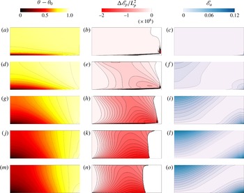
Contour plots of temperature (a,d,g,j,m), change in potential energy
 ${\rm\Delta}\mathscr{E}_{p}/L_{p}^{2}$
(b,e,h,k,n) and available potential density
 $\mathscr{E}_{a}$
(c,f,i,l,o) at different
 $Q$
((a–c)
 $Q=1$
(regime III), (d–f)
 $Q=4$
(regime II), (g–i)
 $Q=10$
(regime II), (j–l)
 $Q=30$
(regime II), (m–o)
 $Q=60$
(regime
 $\text{II}\rightarrow \text{I}$
)) as indicated for Rayleigh number
 $\mathit{Ra}=10^{9}$
, plotted on a meridional cross-section through the centre of the tank. The symmetry axis is at the left of each frame. For
 ${\rm\Delta}\mathscr{E}_{p}/L_{p}^{2}$
, positive values are not shown for clarity. Temperature,
 ${\rm\Delta}\mathscr{E}_{p}/L_{p}^{2}$
and
 $\mathscr{E}_{a}$
are respectively normalised by
 ${\it\delta}{\it\theta}$
,
 ${\it\rho}_{0}{\it\nu}{\it\kappa}/R^{4}$
and
 ${\it\rho}_{0}{\it\nu}{\it\kappa}/gR^{2}$
.

In order to illustrate the effects of rotation on the flow, figure 2 plots the axisymmetric temperature field along with the corresponding available potential density
 $\mathscr{E}_{a}$
at several values of
 $Q$
. Here
 $\mathscr{E}_{a}$
represents the positive-definite spatial contribution of available potential energy, which integrates to
 $E_{a}$
(3.11) (Winters et al.
Reference Winters, Lombard, Riley and D’Asaro1995; Barkan et al.
Reference Barkan, Winters and Smith2013; Winters & Barkan Reference Winters and Barkan2013). Depending on the strength of rotation, the flow can be divided into three regimes (Hussam et al.
Reference Hussam, Tsai and Sheard2014): a rotation-dominated regime at high
 $Q$
where convection in the
 $z$
–
 $r$
plane is suppressed (regime I), a rotation-affected mixed regime (regime II) and a convective regime at low
 $Q$
that is insensitive to rotation (regime III). Hignett et al. (Reference Hignett, Ibbetson and Killworth1981) defined six regimes for rotating horizontal convection: no rotation at
 $Q=0$
; very weak, weak and medium rotation up to
 $Q\sim 1$
(corresponding to Hussam et al.’s regime III); strong rotation for
 $1\ll Q\ll \mathit{Ra}^{4/15}$
(corresponding approximately to regime II); and very strong rotation for
 $Q\gg \mathit{Ra}^{4/15}$
(corresponding approximately to regime I).
Hussam et al. (Reference Hussam, Tsai and Sheard2014) proposed a threshold between regimes III and II of
 $Q_{\text{II-III}}=1$
. Figure 2(a–c) shows an example of a regime III flow at this threshold. The temperature and available potential energy density fields are similar to those of non-rotating horizontal convection, in agreement with experimental results of Hignett et al. (Reference Hignett, Ibbetson and Killworth1981) and numerical results of Sheard & King (Reference Sheard and King2011), Barkan et al. (Reference Barkan, Winters and Smith2013), Hussam et al. (Reference Hussam, Tsai and Sheard2014). This regime is characterised by a thin boundary layer on the base where temperature changes rapidly in the vertical direction, with only minimal variation throughout the interior of the enclosure. The adverse vertical thermal gradient in the forcing boundary layer in regime III is potentially a source of instability via a Rayleigh–Bénard mechanism (Bodenschatz et al.
Reference Bodenschatz, Pesch and Ahlers2000; King & Aurnou Reference King and Aurnou2012). The isotherms depart the bottom wall towards the right (hotter end) before rapidly turning towards the axis, establishing a strong stratification above the forcing boundary. This is due to the strong horizontal boundary layer near the bottom boundary. Almost
 $90\,\%$
of the inner part of the base has isotherms departing the base and terminating at the symmetry axis. The corresponding plot of
 $\mathscr{E}_{a}$
is consistent with figure 8(a) in Barkan et al. (Reference Barkan, Winters and Smith2013), in that available potential energy density is zero everywhere except in close proximity to the corner of the enclosure where destabilising buoyancy is supplied (bottom right here and top right in the Barkan et al. study). The predominance of
 $\mathscr{E}_{a}\approx 0$
is consistent with the corresponding temperature distribution in this case. Available potential energy density is low where fluid is near its equilibrium height, and high otherwise. Here the coolest fluid is located towards the left of the base and is therefore near its equilibrium height, as is the near-uniform-temperature bulk above the bottom boundary layer. However, the hotter fluid near the bottom right corner seeks an equilibrium at the top of the enclosure, resulting in the high
 $\mathscr{E}_{a}$
seen in this region.
For strong rotation cases (regime II) shown in figure 2(d–i), there is still evidence of a horizontal boundary layer above the base, though isotherms are now more strongly inclined with greater vertical temperature variation throughout the enclosure. At
 $Q=4$
(figure 2
d–f), approximately
 $70\,\%$
of the isotherms depart the base and terminate at the symmetry axis. The emergence of the slanted isotherms with temperature gradient inclined upward and away from the axis produces conditions potentially supportive of baroclinic instability (Marshall et al.
Reference Marshall, Jones, Karsten and Wardle2002; Wolfe & Cessi Reference Wolfe and Cessi2010; Lappa Reference Lappa2012; Barkan et al.
Reference Barkan, Winters and Smith2013). Hussam et al. (Reference Hussam, Tsai and Sheard2014) employed the criteria suggested by Hignett et al. (Reference Hignett, Ibbetson and Killworth1981) with
 $\mathit{Pr}=6.14$
and estimated a critical rotation parameter of
 $Q_{c}=2.76$
beyond which baroclinic instability would be anticipated. It would therefore be expected that the temperature fields exhibit characteristics supportive of baroclinic instability at strong and very strong rotations within regime II and I, respectively (Lappa Reference Lappa2012; Barkan et al.
Reference Barkan, Winters and Smith2013; Hussam et al.
Reference Hussam, Tsai and Sheard2014), which will be explained in the next section. Indeed
 $Q=4$
shows that the available potential energy density field is beginning to exhibit the characteristic distribution seen earlier at baroclinically active higher rotation parameters by Barkan et al. (Reference Barkan, Winters and Smith2013), where the higher-
 $\mathscr{E}_{a}$
region at the bottom right corner broadens, and a similarly broad region of higher
 $\mathscr{E}_{a}$
appears at the opposite corner. This is characteristic of the temperature/buoyancy distribution in these cases: the inclination of isotherms creates a radial thermal gradient at all heights. Therefore, near the top of the enclosure the cooler fluid at the left seeks a lower equilibrium height while the warmer fluid at bottom right of the enclosure seeks a higher equilibrium position, leading to the higher
 $\mathscr{E}_{a}$
in these regions, while across a band spanning from the cool bottom left to hot top right of the enclosure, fluid is near its equilibrium height and
 $\mathscr{E}_{a}\approx 0$
.
Figure 2(m–o) shows the flow at
 $Q=60$
, within the rotation-dominated regime I. In this regime the thermal and available potential density fields have reached an asymptotic regime with increasing
 $Q$
. This is characterised by a smooth appearance of the
 ${\it\theta}$
and
 $\mathscr{E}_{a}$
contours, reflecting the suppression of horizontal convection in the
 $z$
–
 $r$
plane. In contrast, the corresponding fields in regime II, depicted at
 $Q=4$
, 10 and 30 in figure 2(d–i), exhibit small-scale deviations towards the hotter end of the enclosure: near the bottom wall at lower
 $Q$
, and more visible towards the enclosure side wall at
 $Q=10$
and 30.
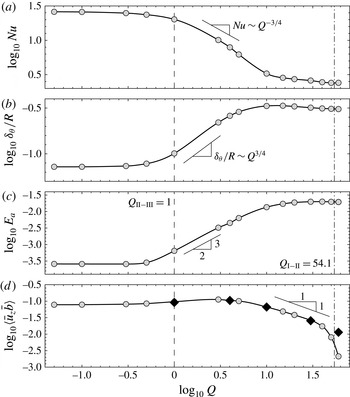
Plots of (a)
 $\log _{10}\mathit{Nu}$
, (b)
 $\log _{10}{\it\delta}_{{\it\theta}}/R$
, (c)
 $\log _{10}E_{a}$
and (d)
 $\log _{10}\langle \bar{u}_{z}\bar{b}\rangle$
against
 $\log _{10}Q$
for saturated axisymmetric flows at
 $\mathit{Ra}=10^{9}$
and
 $\mathit{Pr}=6.14$
.
 $E_{a}$
is normalised by
 ${\it\rho}_{0}R{\it\nu}{\it\kappa}$
and
 $\langle \bar{u}_{z}\bar{b}\rangle$
by
 ${\it\nu}^{2}{\it\kappa}/R^{4}$
. In (d), black diamond symbols show
 $\log _{10}({\it\kappa}/H){\rm\Delta}\hat{b}$
. The regime thresholds
 $Q_{\text{II-III}}=1$
and
 $Q_{\text{I-II}}=54.1$
from Hussam et al. (Reference Hussam, Tsai and Sheard2014) are included for reference, and are respectively shown by vertical dashed and dash-dot lines. Gradient indicators are included for guidance where the data is consistent with Stern’s scaling (a,b) or where it may locally support a power-law scaling (c,d).

A consequence of the suppression of horizontal convection with increasing
 $Q$
is a corresponding decrease in Nusselt number characterising the transfer of heat through the base (Hussam et al.
Reference Hussam, Tsai and Sheard2014). Here Nusselt number is defined as the heat flux relative to that due to conduction following convention in horizontal convection (e.g. Mullarney et al.
Reference Mullarney, Griffiths and Hughes2004; Hussam et al.
Reference Hussam, Tsai and Sheard2014),
 $$\begin{eqnarray}\mathit{Nu}=\overline{\left|{\displaystyle \frac{\partial {\it\theta}}{\partial z}}\right|}\frac{R}{{\it\delta}{\it\theta}},\end{eqnarray}$$
where
 $\overline{\,\left|\partial {\it\theta}/\partial z\right|}$
is the integral of the absolute value of temperature flux over the base, and the combination of a vertical heat flux with a horizontal conduction scale mean that this definition does not follow
 $\mathit{Nu}\rightarrow 1$
with vanishing convection.
It would be expected that in the low-
 $Q$
regime III the Nusselt number would be constant and consistent with that of the non-rotating case for the given Rayleigh number, while in the high-
 $Q$
regime I the Nusselt number would adhere to the low-
 $\mathit{Ra}$
value in the non-rotating system due to the aforementioned suppression of horizontal convection. The intermediate regime II would then see a decrease in
 $\mathit{Nu}$
with increasing
 $Q$
to bridge the two asymptotic regimes. Hussam et al. (Reference Hussam, Tsai and Sheard2014) showed for higher rotation parameters that rotating radial convection demonstrated behaviour consistent with a scaling proposed by Stern (Reference Stern1975). Stern developed a scaling for thermal boundary layer thickness (
 ${\it\delta}_{{\it\theta}}$
) in rotating horizontal convection which using the present nomenclature is
 ${\it\delta}_{{\it\theta}}/R=Q^{3/4}\mathit{Ra}^{-1/5}$
. Given that
 $\mathit{Nu}\sim R/{\it\delta}_{{\it\theta}}$
, the corresponding Nusselt number scaling is
 $\mathit{Nu}\sim Q^{-3/4}\mathit{Ra}^{1/5}$
. Figure 3(a) plots logarithms of
 $\mathit{Nu}$
and
 ${\it\delta}_{{\it\theta}}/R$
against the logarithm of
 $Q$
. Immediately apparent is an asymptotic behaviour in
 $\mathit{Nu}$
and
 ${\it\delta}_{{\it\theta}}/R$
as both
 $Q\rightarrow 0$
and
 $\rightarrow \infty$
. Furthermore, the expected decrease in
 $\mathit{Nu}$
and increase in
 ${\it\delta}_{{\it\theta}}/R$
at intermediate
 $Q$
is observed. The bulk of the decrease in Nusselt number occurs over
 $1\lesssim Q\lesssim 10$
, and throughout this range the decrease closely follows the
 $\mathit{Nu}\sim Q^{-3/4}$
scaling of Stern (Reference Stern1975).
Hussam et al. (Reference Hussam, Tsai and Sheard2014) proposed a threshold between regimes I and II at higher rotation parameters where they found the Stern scaling to hold, given by
 $Q_{\text{I-II}}=0.215\mathit{Ra}^{4/15}$
. This threshold has the same form as the very strong rotation threshold given by Hignett et al. (Reference Hignett, Ibbetson and Killworth1981). The threshold was taken as the value of
 $Q$
where the Nusselt number first reached its high-
 $Q$
asymptotic value. Extrapolating to the present conditions (
 $\mathit{Ra}=10^{9}$
), Hussam et al.’s threshold predicts
 $Q_{\text{I-II}}=54.1$
. Their threshold was estimated using data acquired only up to
 $Q=1.59$
at
 $\mathit{Ra}=10^{9}$
, so its applicability to the rotation parameters
 $Q\gg 1$
traversed in the present study is unknown. In figure 3(a), Nusselt number decreases steeply in accordance with the
 $\mathit{Nu}\sim Q^{-3/4}$
scaling only up to
 $Q\approx 10$
. Beyond this, only a gradual decrease in Nusselt number is observed towards the high-
 $Q$
asymptotic value. Stern’s scaling relies on the thickness of the thermal boundary layer being much less than the enclosure height, i.e.
 ${\it\delta}_{{\it\theta}}\ll H$
. This condition breaks down at
 $Q\approx 10$
, impeding further growth in
 ${\it\delta}_{{\it\theta}}$
with increasing
 $Q$
(and thus impeding further reduction in
 $\mathit{Nu}$
). Nevertheless, the data in figure 3(a) reaches constant values at high
 $Q$
for
 $Q\gtrsim 50$
. Inspecting figure 4(b) in Hussam et al. (Reference Hussam, Tsai and Sheard2014) demonstrates that while the departure of
 $\mathit{Nu}$
from its regime I value occurs at
 $\log _{10}\!\left(Q^{-3/4}\mathit{Ra}^{1/5}\right)\approx 0.5$
, it reaches the power-law dependence on
 $Q^{-3/4}\mathit{Ra}^{1/5}$
predicted by Stern at
 $\log _{10}\!\left(Q^{-3/4}\mathit{Ra}^{1/5}\right)\approx 1$
. This corresponds to
 $Q\approx 12$
, close to the
 $Q\approx 10$
value at which the
 $\mathit{Nu}\sim Q^{-3/4}$
behaviour seen in figure 3(a) ceases. These results combine to verify that the scaling proposed by Stern persists to the high
 $Q$
range of the present study. However, it should be noted that baroclinic eddies will play a key role in determining the depth of the thermal boundary layer in the three-dimensional (non-axisymmetric) flow (Cessi & Fantini Reference Cessi and Fantini2004; Barkan et al.
Reference Barkan, Winters and Smith2013), which is likely to disrupt the scaling underpinning the
 $Q_{\text{I}-\text{II}}$
threshold discussed here. The linear stability of the baroclinically active flows will be explored in § 5.
It is pertinent to briefly discuss the role of the height ratio in determining the regime thresholds (Sheard & King Reference Sheard and King2011). The threshold between regimes III and II represents the point at which rotation effects begin to modify Rossby’s (Reference Rossby1965) scaling for the horizontal convection boundary layers valid at low rotations (
 $Q<O(1)$
), producing a thicker thermal layer on the base and smaller Nusselt numbers. Both Rossby’s and Stern’s scalings require the boundary layer to be much thinner than the enclosure height: hence at a sufficiently low Rayleigh number, the layers will interfere with the limited enclosure height, suppressing the rotation-affected regimes II and III altogether. Smaller height ratios require higher Rayleigh numbers to produce the sufficiently thin boundary layers to avoid this interference. This effect is amplified at higher
 $Q$
, as under Stern’s scaling the boundary layer is relatively thicker than the corresponding horizontal convection layer under weak rotation (scaling with
 $Q^{3/4}\mathit{Ra}^{-1/5}$
rather than
 $\mathit{Ra}^{-1/5}$
). Hence even higher Rayleigh numbers would be required to produce distinct boundary layers at smaller height ratios under stronger rotation.
The available potential energy density plots in figure 2 exhibited an increase in both the strength and extent of
 $\mathscr{E}_{a}$
across the flow. This observation is supported quantitatively by figure 3(c), which relates the total available potential energy (
 $E_{a}$
) to
 $Q$
.
 $E_{a}$
is low and constant in regime III at low
 $Q$
, and increases monotonically throughout regime II. As indicated in the figure, the data follows an approximate scaling
 $E_{a}\sim Q^{3/2}$
within this regime over
 $O(1)<Q<O(10)$
. Beyond
 $Q\approx 10$
, the rate of increase of
 $E_{a}$
becomes shallower, before it ultimately plateaus towards the high-
 $Q$
regime.
Barkan et al. (Reference Barkan, Winters and Smith2013) showed that advection dominated the horizontal buoyancy flux at low rotation parameters, while diffusion dominated at high rotations. The present axisymmetric solutions support this: figure 2 shows that lateral thermal gradients are low at small
 $Q$
(corresponding to small lateral diffusive buoyancy flux), and become more pronounced as the isotherms begin inclining from the near horizontal at low
 $Q$
towards the vertical at high
 $Q$
(supporting stronger diffusive lateral buoyancy flux). Simultaneously, with increasing
 $Q$
, the progressive suppression of lateral heat and mass transport via horizontal convection achieves the switch from advective to diffusive lateral buoyancy flux with increasing
 $Q$
. Winters & Young (Reference Winters and Young2009) presented the volume-averaged potential energy equation applicable to horizontal convection, which can be used to show (Barkan et al.
Reference Barkan, Winters and Smith2013) that at saturation, the volume-averaged vertical buoyancy flux
 $\langle \bar{u}_{z}\bar{b}\rangle$
is proportional to the difference between the mean buoyancy at the top and bottom boundaries (
 ${\rm\Delta}\hat{b}$
) through
 $\langle \bar{u}_{z}\bar{b}\rangle =({\it\kappa}/H){\rm\Delta}\hat{b}$
. In figure 3(d) the variation of vertical buoyancy flux with
 $Q$
is plotted. The flux is strong at low
 $Q$
, before elevating slightly up to its maximum value at
 $Q\approx 3$
. It subsequently decreases as
 $Q$
is increased further. Over
 $5\lesssim Q\lesssim 30$
this decrease approximately follows a power law
 $\langle \bar{u}_{z}\bar{b}\rangle \sim Q^{-1}$
, and thereafter the rate of decrease accelerates rapidly as the very strongly rotating regime is reached. Competing effects combine to produce the observed behaviour. The shift from the horizontally stratified low-
 $Q$
state to a predominantly horizontal thermal gradient with increasing
 $Q$
places cooler fluid nearer the axis where downwelling occurs and warmer fluid towards the side wall where fluid is transported upwards, which serves to enhance vertical buoyancy flux. Conversely, as
 $Q$
is increased from the non-rotating scenario, the suppression of horizontal convection serves to reduce the vertical buoyancy flux. While the former effect is stronger at lower
 $Q$
leading to the slight increase in
 $\langle \bar{u}_{z}\bar{b}\rangle$
up to
 $Q\approx 3$
, at higher
 $Q$
the arrest of horizontal convection overturning in the
 $z$
–
 $r$
plane reduces and ultimately suppresses
 $\langle \bar{u}_{z}\bar{b}\rangle$
.
Figure 3(d) also includes calculations of
 $({\it\kappa}/H){\rm\Delta}\hat{b}$
for the
 $5$
cases shown in figure 2. The average buoyancy at the bottom boundary was calculated analytically using the prescribed thermal boundary condition
 $$\begin{eqnarray}\hat{b}_{z=0}=\frac{2{\rm\pi}{\it\alpha}g}{{\rm\pi}R^{2}}\int _{0}^{R}r\,\bar{{\it\theta}}_{z=0}\,\text{d}r=\frac{2}{3}{\it\alpha}g\,{\it\delta}{\it\theta},\end{eqnarray}$$
while at the top boundary it was approximated using a trapezoidal quadrature rule employing a very large number of intervals (
 $N=999$
intervals;
 $1000$
sample points) interpolated at spectral accuracy from the high-order temperature field solution,
 $$\begin{eqnarray}\hat{b}_{z=H}\approx \frac{2{\rm\pi}{\it\alpha}g}{{\rm\pi}R^{2}}\frac{R}{N}\left[\frac{R\,\bar{{\it\theta}}_{z=H,r=R}}{2}+\mathop{\sum }_{k=1}^{N-1}\frac{kR}{N}\,\bar{{\it\theta}}_{z=H,r=kR/N}\right].\end{eqnarray}$$
Calculations of the integrals were repeated with
 $500$
points, and these agreed to between
 $5$
and
 $7$
significant figures, verifying the accuracy of the quadrature estimates. A very close agreement between the
 $\langle \bar{u}_{z}\bar{b}\rangle$
and
 $({\it\kappa}/H){\rm\Delta}\hat{b}$
data is seen up to
 $Q=30$
. However, at
 $Q=60$
 $\langle \bar{u}_{z}\bar{b}\rangle$
drops below the
 $({\it\kappa}/H){\rm\Delta}\hat{b}$
values, which are observed continuing to follow the aforementioned
 $Q^{-1}$
scaling trend. This discrepancy appears at the highest
 $Q$
investigated, and where the buoyancy flux is smallest, so may reflect a difficulty in accurately capturing the buoyancy flux when the advective transport in the
 $z$
–
 $r$
plane becomes very weak. Nevertheless, the observed agreement confirms that the relation obtained from the potential energy equation for horizontal convection (Winters & Young Reference Winters and Young2009; Barkan et al.
Reference Barkan, Winters and Smith2013) at steady state extends to radial horizontal convection with rotation in cylindrical enclosures.
Hussam et al. (Reference Hussam, Tsai and Sheard2014) demonstrated that a consequence of the radial horizontal convection combined with the system rotation is the development of an azimuthal swirl in the interior exceeding the background rotation rate. This incites azimuthal shear at the enclosure side wall that may promote non-axisymmetric instability through mechanisms such as centrifugal instability (Lopez & Marques Reference Lopez and Marques2009; Lopez, Marques & Avila Reference Lopez, Marques and Avila2013; Curbelo et al. Reference Curbelo, Lopez, Mancho and Marques2014), or Stewartson layer instabilities (Stewartson Reference Stewartson1957; Hide & Titman Reference Hide and Titman1967; Niino & Misawa Reference Niino and Misawa1984; Vo et al. Reference Vo, Montabone and Sheard2014, Reference Vo, Montabone and Sheard2015). The next section describes the linear stability analysis performed to elucidate the instability mechanisms active in the rotating radial horizontal convection system.
5 Linear stability of the axisymmetric base flows
Growth rates of the leading eigenmode as a function of azimuthal wavenumber were obtained across a wide range of rotation parameter
 $0\leqslant Q\leqslant 60$
. The leading eigenmode was found to be consistently complex across the
 $Q$
–
 ${\it\beta}$
parameter space. A map of instabilities in the
 $Q$
–
 ${\it\beta}$
parameter space was constructed from stability calculations performed at over
 $300$
 $Q$
–
 ${\it\beta}$
combinations at
 $\mathit{Ra}=10^{9}$
and
 $\mathit{Pr}=6.14$
. A marginal stability envelope was obtained by interpolating for the values of
 ${\it\beta}$
giving zero growth rate. The loci of peak growth rate for distinct instability modes branches were extracted, and the instability mode were classified by inspection of their respective eigenmodes.
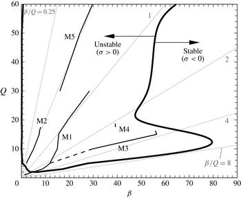
Neutral stability (solid line) and loci of maximum growth rate (dashed lines) for the
 $5$
identified mode branches (labelled) across the
 $Q$
–
 ${\it\beta}$
parameter space for
 $\mathit{Ra}=10^{9}$
and
 $\mathit{Pr}=6.14$
. For guidance, the data are plotted over faint radial lines of constant
 ${\it\beta}/Q$
, with values doubling in the clockwise direction from
 ${\it\beta}/Q=0.25$
to
 $8$
.

Figure 4 plots the marginal stability curve for
 $Q\leqslant 60$
. Everywhere inside the marginal stability curve, the growth rate is positive and hence the flow is unstable to infinitesimal disturbances of the enclosed azimuthal wavenumbers. Five distinct instability mode branches have been identified in the
 $Q$
–
 ${\it\beta}$
parameter space. Below
 $Q=1.86$
the flow is stable. At
 $Q=1.86$
, instability first emerges with an azimuthal wavenumber
 ${\it\beta}\approx 5$
. The domain of unstable wavenumbers widens rapidly with increasing
 $Q$
up to
 $Q\approx 12$
, with instability growth predicted across
 $0\lesssim {\it\beta}\lesssim 80$
. The band of unstable wavenumbers contracts to
 ${\it\beta}\approx 48$
at
 $Q\approx 20$
, and a gradual monotonic increase is observed thereafter, passing
 ${\it\beta}\approx 64$
at
 $Q=60$
. The asymptotic state for high
 $Q$
appears to be a single instability mode branch of more modest wavenumber, ranging from
 ${\it\beta}\approx 15$
at
 $Q=30$
to
 ${\it\beta}\approx 30$
at
 $Q=60$
.
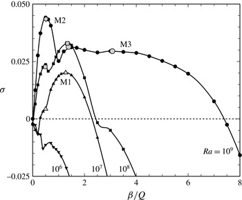
A plot of
 ${\it\sigma}$
scaled by
 ${\it\nu}/R^{2}$
against
 ${\it\beta}/Q$
for the dominant eigenvalue at each wavenumber at
 $Q$
values as shown. Line dash length and line thickness increase with increasing
 $Q$
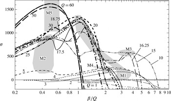
to aid reading of the plot, and the actual computed eigenvalues are represented by symbols. Shaded regions contain the local maxima corresponding to each mode branch identified in this study, as labelled.

A feature that emerges from figure 4 is that the loci of maximum growth, and indeed the neutral stability boundary over
 $2\lesssim Q\lesssim 10$
, lie approximately along radial lines extending from the origin (or in other words, along lines of constant
 ${\it\beta}/Q$
). In figure 5 the growth rate of the dominant eigenvalue (
 ${\it\sigma}$
) is plotted against this scaled wavenumber (
 ${\it\beta}/Q$
). In this plot the growth rate has been re-scaled: under the normalisation described in § 3, the physical growth rate is normalised by
 ${\it\Omega}$
, whereas here it is scaled by
 ${\it\nu}/R^{2}$
. Under close inspection, this figure reveals subtleties in the alteration in the flow stability with changing
 $Q$
.
Beginning with the M1 branch, a stable local maximum is seen at
 $Q=1$
and
 ${\it\beta}/Q\approx 1.2$
, which by
 $Q=2$
has just become unstable, with peak growth rate occurring at
 ${\it\beta}/Q\approx 2.6$
. By
 $Q=3$
, the growth rate is stronger, with a peak at
 ${\it\beta}/Q\approx 3$
, and maxima corresponding to this branch are observed up to
 $Q=5$
, with monotonically increasing growth rate. A retreat in peak scaled wavenumber back to
 ${\it\beta}/Q\approx 2.5$
is found over this increase in
 $Q$
, which reflects the positive curvature in
 $Q$
–
 ${\it\beta}$
space for the M1 branch seen in figure 4. The mode exhibits an increase in growth rate and reduction in
 ${\it\beta}/Q$
, having
 ${\it\beta}/Q\approx 1.4$
at
 $Q=10$
.
 $Q=5$
is also notable for the appearance of a second peak exhibiting weaker growth rates at a lower
 ${\it\beta}/Q\approx 0.4$
: this peak marks the inception of the M2 branch.
The M2 branch is dominant at
 $Q=10$
, and exhibits little change in peak growth rate or scaled peak wavenumber (
 ${\it\beta}/Q\approx 0.5$
) over
 $10\leqslant Q\leqslant 17.5$
. However, the M1 branch at
 $Q=15$
and beyond consistently achieves a higher peak growth rate than the M2 branch. In fact, in the vicinity of
 $0.5\lesssim {\it\beta}/Q\lesssim 0.7$
evidence of an erosion of the M2 local maxima from the higher-wavenumber side is observed with increasing
 $Q$
. From
 $Q=16.5$
to
 $17.5$
, the M2 local maximum vanishes due to encroachment of the waveband of the higher-wavenumber M1 branch. This suppression of a low-wavenumber mode persists through to
 $Q=25$
, but by
 $Q=30$
, a peak with
 ${\it\beta}/Q\approx 0.5$
corresponding to the M5 branch appears. This branch is weaker than the higher-wavenumber M1 branch at
 $Q=30$
, but at higher
 $Q$
the higher-wavenumber mode peaks vanish, leaving the M5 branch as the sole branch for
 $Q\gtrsim 50$
.
Between
 $Q=10$
and
 $17.5$
, the higher-wavenumber M3 branch is also found at
 ${\it\beta}/Q\approx 3.8$
. This mode is notable in that its peak growth rate is almost independent of
 $Q$
. Beyond
 $Q=16.25$
the M3 branch too gives way as the maximum scaled wavenumber producing unstable eigenmodes contracts from
 ${\it\beta}/Q\approx 7.4$
at
 $Q=10$
to
 ${\it\beta}/Q\approx 2.8$
at
 $Q=17.5$
. The final mode branch found in this study is M4, which exists as a small local maximum at
 ${\it\beta}/Q\approx 2.2$
and
 $17.5\lesssim Q\lesssim 18.75$
. However, with a growth rate
 ${\it\sigma}\approx 230$
, this mode is insignificant against the M1 branch (
 ${\it\sigma}>1200$
) at these
 $Q$
values.
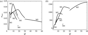
Plots of maximum growth rate
 ${\it\sigma}_{max}$
against
 $Q$
for each identified mode branch. Panels (a) and (b) show
 ${\it\sigma}_{max}$
respectively scaled by
 ${\it\Omega}$
and
 ${\it\nu}/R^{2}$
.

Figure 6 distils the maximum growth rate of each of the mode branches against
 $Q$
, using both the native
 ${\it\Omega}$
-scaling as well as the alternative
 ${\it\nu}/R^{2}$
scaling employed in figure 5. Considering figure 6(b), with increasing
 $Q$
the growth rate progressively increases, with each of the mode peaks observed in figure 6(a) emerging with a rapid increase in growth rate before plateauing and being replaced by a subsequent mode: first the M1 mode emerges at
 $1.86$
, before being surpassed by the M2 mode at
 $Q\approx 5$
, which is overtaken by the M1 branch again at
 $Q\approx 14$
. The M1 branch reaches a peak growth rate at
 $Q\approx 20$
before gradually reducing and being replaced by the M5 branch at higher
 $Q$
. The growth rate appears to plateau at
 ${\it\sigma}\approx 1.6\times 10^{3}$
beyond
 $Q\approx 55$
. This corresponds to the very strongly rotating regime I described in § 4, in which the underlying axisymmetric base flows reach an asymptotic state invariant with further increases in
 $Q$
. It is therefore expected that no additional instability modes will manifest beyond the range
 $Q\leqslant 60$
investigated in this study. This assertion is supported by the single maximum in the
 ${\it\sigma}$
–
 ${\it\beta}$
data presented for
 $Q=50$
and
 $60$
in figure 5.
Characterisation of, and elaboration on, each of the mode branches shown in figure 4 is provided in the subsections to follow.
5.1 Eigenmode energetics along instability mode branches
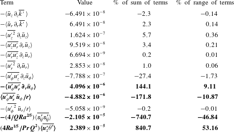
Along each of the mode branches revealed in figures 4 and 6, the energetics of the azimuthally averaged eigenvector fields were analysed by evaluating each term of equation (3.19). In every case considered in this work, the same four terms consistently had the largest magnitudes across the
 $12$
calculated terms: the next largest term was at most
 $5\,\%$
of the dominant term in all cases, with a mean of
 $2.1\,\%$
. As an example, table 2 displays the computed integral summations of each term for the leading instability mode at
 $Q=5$
and
 $k=12$
, with the dominant terms highlighted.
Volume integrated values of terms in (3.19) for the leading instability eigenmode with
 ${\it\beta}=12$
for a flow with
 $Q=5$
and
 $\mathit{Ra}=10^{9}$
. The integrated term values are scaled by
 $R^{5}{\it\Omega}^{3}$
. For each term, the two right-most columns respectively include the percentage contributions of each term to the sum and range (
 $\max {-}\min$
) of the terms contributing to
 $\partial _{t}\overline{k^{\,\prime }}$
. Highlighted in bold are the four terms of largest absolute value contribution.

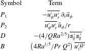
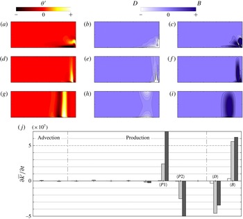
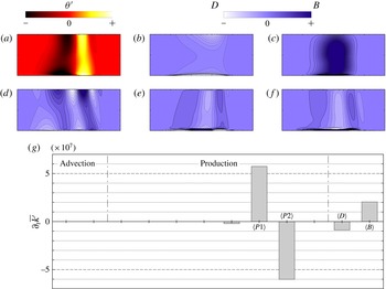
For brevity, nomenclature is assigned to each of the four dominant terms, as per table 3. The first two terms describe the production of perturbation kinetic energy in the
 $r$
-
 ${\it\theta}$
plane due respectively to horizontal shear in, and azimuthal rotation of, the base flow, and are denoted by
 $P_{1}$
and
 $P_{2}$
. The third term, denoted by
 $D$
, describes the viscous dissipation of perturbation kinetic energy and the fourth term, denoted by
 $B$
, describes the transfer from perturbation potential energy to kinetic energy. Note that due to the absence of the integration operators
 $\langle \cdots \,\rangle$
from the terms in table 3 compared to the corresponding terms in table 2,
 $P_{1}$
,
 $P_{2}$
,
 $D$
and
 $B$
each represent a spatially varying field on the
 $z$
–
 $r$
plane.
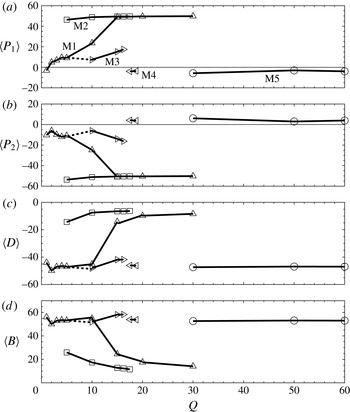
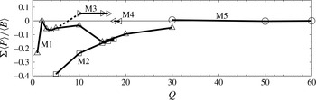
(a–d) Plots of the respective percent-of-range contributions of
 $\langle P_{1}\rangle$
,
 $\langle P_{2}\rangle$
,
 $\langle D\rangle$
and
 $\langle B\rangle$
against
 $Q$
, for each of the mode branches identified in figure 4.


Percent-of-range contributions of each of the four dominant terms were evaluated along the loci of maximum growth rate for the mode branches from figures 4 and 6. These are plotted in figure 7. Several different instability behaviours are suggested by the markedly different proportional contributions of the four dominant terms in these plots:
-
(1) At both
$Q\gtrsim 30$
(M5) and
$Q\approx 18$
(M4), the two production terms
$\langle P_{1}\rangle$
and
$\langle P_{2}\rangle$
are weakly negative and positive, respectively (magnitudes being less than approximately
$6\,\%$
), and sum to approximately zero. The dissipation term
$\langle D\rangle$
is strongly negative (
${\approx}-47\,\%$
), while the buoyancy term
$\langle B\rangle$
is slightly stronger (
${\approx}52\,\%$
) and positive. -
(2) The M1 and M3 modes at smaller
$Q$
values exhibit similar proportions to M4 and M5 for the
$\langle D\rangle$
and
$\langle B\rangle$
terms, but are notably different in the production terms. In addition to being stronger (M1 and M2 having production term magnitudes up to
$12\,\%$
and
$18\,\%$
, respectively), the terms are opposite-signed, with
$\langle P_{1}\rangle$
predominantly positive and
$\langle P_{2}\rangle$
negative. -
(3) The M2 mode is different again: production terms
$\langle P_{1}\rangle$
and
$\langle P_{2}\rangle$
are strong (
${\approx}50\,\%$
), with
$\langle P_{1}\rangle$
positive and
$\langle P_{2}\rangle$
negative. This mode exhibits the weakest proportions of dissipation (between
$-7\,\%$
and
$-14\,\%$
) and buoyancy (between approximately
$12\,\%$
and
$25\,\%$
) amongst all mode branches. -
(4) The M1 mode exhibits the most significant change in the relative contributions of the terms over intermediate
$Q$
values
$5\lesssim Q\lesssim 15$
. At low
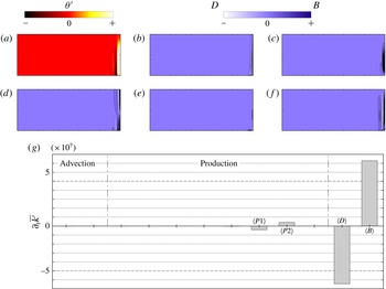
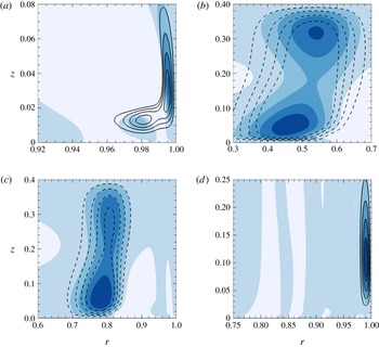
$Q$
, the mode exhibits modest production term contributions, a strong negative dissipation contribution, and a stronger positive buoyancy contribution, while at higher
$Q$
, the distribution is similar to the M2 mode.


In order to confirm if the categorisation of instability modes based on their energetics is valid, attention is turned to the eigenvector fields in the subsections to follow.
5.2 Eigenmode structure and dominant energetics fields
The first mode branch to be considered is the M1 branch. In contrast to the other mode branches described herein, the energetics analysis in figure 7 shows that the M1 branch experiences a significant change in the proportional contributions of individual terms to the evolution of azimuthally averaged perturbation kinetic energy as a function of
 $Q$
: when
 $Q\lesssim 5$
the M1 branch has energy evolution contributions consistent with the M3 branch; the shift in the distribution of contributions occurs over
 $5\lesssim Q\lesssim 15$
; and for
 $Q\gtrsim 15$
the M1 branch has energy evolution contributions resembling the M2 branch. Figure 8 illustrates the eigenmode structure and the integral contributions of all
 $12$
terms from table 3 for the M1 branch at values of
 $Q$
capturing each of the aforementioned behaviours.
(a–i) Structure of the M1 eigenmode; contour plots of perturbation temperature, azimuthally averaged perturbation kinetic energy evolution viscous dissipation (
 $D$
) and available potential energy conversion fields (
 $B$
) at
 $Q$
and
 ${\it\beta}$
as shown. Arbitrary contour levels equispaced about zero are plotted to elucidate the perturbation field structure. For each
 $Q$
–
 ${\it\beta}$
combination, the same contour levels are used for
 $D$
and
 $B$
fields. (j) Plots the integral contributions of each of the terms contributing to the azimuthally averaged perturbation kinetic energy equation, for each of the
 $Q$
–
 ${\it\beta}$
combinations in (a–i). White, light grey and dark grey bars represent (a–c)
 $Q=2,{\it\beta}=5^{\circ }$
, (d–f)
 $Q=10,{\it\beta}=15^{\circ }$
, and (g–i)
 $Q=20,{\it\beta}=20^{\circ }$
, respectively. From left to right, the plot follows the order of terms shown in table 2, while the four dominant terms,
 $\langle P1\rangle$
,
 $\langle P2\rangle$
,
 $\langle D\rangle$
and
 $\langle B\rangle$
are labelled. The first two terms arise from advection of
 $\overline{k^{\,\prime }}$
on the mean flow, the next
 $8$
terms arise from production of
 $\overline{k^{\,\prime }}$
due to velocity shear, as labelled. The contributions to
 $\partial \overline{k^{\,\prime }}/\partial t$
are scaled by
 ${\it\nu}^{3}/R^{4}$
.

The first case,
 $Q=2$
and
 ${\it\beta}=5$
, demonstrates that the eigenmode is concentrated adjacent to the hot outer part of the forcing boundary and up the outer side wall (occupying approximately the outer radial
 $25\,\%$
of the base and lower
 $40\,\%$
of the side wall). This is reflected by the
 ${\it\theta}^{\prime }$
,
 $D$
and
 $B$
fields shown in figure 8(a–i). The dissipation field
 $D$
is strongest at the boundaries in the vicinity of the junction between base and side wall. This behaviour is consistent with dissipation due to viscous shear in perturbation velocity boundary layers in this vicinity. In terms of the
 $B$
field, regions of high production extend from the hot corner. At
 $Q=2$
, the mode is only very weakly unstable (ref. the small positive peak growth rate in figure 5). Correspondingly, in figure 8(j) the integrals of the two dominant terms,
 $D$
and
 $B$
, are seen to be approximately equal and opposite.
In the region of shifting mode behaviour (
 $Q=10$
and
 ${\it\beta}=15$
, figure 8
d–f), the eigenmode is found to become narrower and extend further in the vertical direction. In notable contrast to the
 $Q=2$
case, here the perturbation field structure is displaced from the side wall, the dissipation field
 $D$
is again strongest at the bottom boundary at the same location as the temperature field features and the
 $B$
field is dominated by a region of strong energy production extending vertically from the base through much of the interior. At
 $Q=20$
, the eigenmode structure is positioned at approximately
 $80\,\%$
of the tank radius from the axis. The
 $B$
field exhibits a similar dominant vertical structure to the
 $Q=10$
case, but the structure is broader.
In figure 8(j) the production term contributions
 $\langle P1\rangle$
and
 $\langle P2\rangle$
are consistently positive and negative, respectively, and approximately cancel. While not shown in this paper, the authors consistently found the fields for the
 $P1$
and
 $P2$
production terms to be similarly structured, but opposite signed. Hence the
 $P1$
and
 $P2$
fields typically sum to approximately zero both locally and globally. With increasing
 $Q$
, the M1 branch exhibits a strong increase in the magnitude of
 $\langle P1\rangle$
and
 $\langle P2\rangle$
. At
 $Q=2$
, the
 $\langle D\rangle$
and
 $\langle B\rangle$
contributions have a significantly greater magnitude than
 $\langle P1\rangle$
and
 $\langle P2\rangle$
, but by
 $Q=20$
this is reversed.
The M2 branch is represented at
 $Q=10$
with dominant wavenumber
 ${\it\beta}=5$
in figure 9. In figure 9(a–f), fields
 ${\it\theta}^{\prime }$
,
 $D$
and
 $B$
are plotted, along with the axial, radial and azimuthal components of vorticity in the eigenvector field (
 ${\it\omega}_{z}^{\prime }$
,
 ${\it\omega}_{r}^{\prime }$
and
 ${\it\omega}_{{\it\phi}}^{\prime }$
, respectively). Strong similarities are observed between the M2 branch eigenmode visualised here and the M1 branch at
 $Q=20$
in figure 8 (moreover, the energetics data in figure 7 indicates that the behaviour at
 $Q=20$
will be maintained over
 $15\lesssim Q\lesssim 30$
). However, here the M2 eigenmode structures are approximately three times broader than the
 $Q=20$
M1 eigenmode, likely reflecting the lower dominant wavenumbers of the M2 branch (here
 ${\it\beta}=5$
) in comparison to the M2 branch beyond
 $Q\approx 15$
(
 ${\it\beta}\gtrsim 15$
).
Representative structure of the M2 eigenmode at
 $Q=10$
and
 ${\it\beta}=5$
. (a–f) Plots fields of
 ${\it\theta}^{\prime }$
,
 $D$
,
 $B$
and perturbation vorticity components
 ${\it\omega}_{z}^{\prime }$
,
 ${\it\omega}_{r}^{\prime }$
and
 ${\it\omega}_{{\it\phi}}^{\prime }$
. For
 ${\it\theta}^{\prime }$
,
 $D$
and
 $B$
, contour levels and shading are as per figure 8. The same set of arbitrary contour levels are used for each vorticity component. (g) Plots contributions to
 $\partial _{t}\overline{k^{\,\prime }}$
as per figure 8.

The perturbation kinetic energy contributions plotted in figure 9(b) demonstrate that the production terms sum to a weakly negative contribution. The gain from
 $\langle B\rangle$
is more than twice the deficit due to viscous dissipation through
 $\langle D\rangle$
, reflecting the importance of
 $\langle B\rangle$
to the instability growth. The spatial distribution of
 $B$
reveals that this conversion of perturbation available potential energy to kinetic energy is strongest in a broad region extending almost the full depth of the enclosure at approximately
 $50\,\%$
of the radial distance from the axis. The vorticity fields reveal alternating-sign axial vorticity structures extending from the top to the base of the enclosure. The radial and azimuthal vorticity fields are both strongest in a thin layer adjacent to the bottom wall, which the
 $D$
field in figure 9(a–f) demonstrates is responsible for significant viscous dissipation, but because it is localised to a slender region, its integral
 $\langle D\rangle$
is modest, and does not inhibit instability growth. Revisiting the axisymmetric base flow for this case with
 $Q=10$
depicted in figure 2(g–i), the region occupied by the eigenmode structures has inclined isotherms with thermal gradient directed diagonally upward and radially outward. Under rotation, this flow pattern is susceptible to baroclinic instability, and the change in potential energy field
 ${\rm\Delta}\mathscr{E}_{p}$
in figure 2(g–i) is indeed found to be strongly negative in the region occupied by the eigenmode structures, supporting the assertion that this instability mode has a baroclinic origin. Furthermore, the available potential energy density field
 $\mathscr{E}_{a}$
for the axisymmetric base flow demonstrates that the flow has accumulated a significant amount of potential energy that cannot be released into the axisymmetric flow, but is available for release to the non-axisymmetric (three-dimensional) modes. Barkan et al. (Reference Barkan, Winters and Smith2013) demonstrated using numerical simulation that two-dimensional rotating horizontal convection in a rectangular enclosure accumulated significantly more available potential energy than its three-dimensional counterpart. The present results demonstrate a global linear instability mode with baroclinic features that may facilitate a conversion of accumulated axisymmetric available potential energy to perturbation kinetic energy in a non-axisymmetric flow state.
Representative structure of the M5 eigenmode at
 $Q=50$
and
 ${\it\beta}=25$
. Contour levels and shading are as per figure 9.

A representative eigenmode from the M5 branch is displayed in figure 10 for
 $Q=50$
and
 ${\it\beta}=25$
. Figure 10(g) demonstrates the unusual feature amongst these mode branches that
 $\langle P1\rangle <0$
and
 $\langle P2\rangle >0$
which is contrary to all but the fleeting M4 branch. The eigenmode structures are concentrated in a narrow region adjacent to the side wall. The radial vorticity component is small compared to the axial and azimuthal components, both of which are prominent.

In addition to thermal instability mechanisms, consideration was also given to the possibility that hydrodynamic shear-layer instabilities may play a role in this system. For instance, the development of swirling flow about a vertical axis of rotation may invite shear-layer instabilities on horizontal planes. The Rayleigh–Kuo criterion (Rayleigh Reference Rayleigh1879; Kuo Reference Kuo1949) is a necessary but not sufficient condition for instability that requires the horizontal gradient of absolute vorticity to change sign somewhere within the domain. The base flows obtained in § 4 were tested at various depths across the investigated range of
 $Q$
against the Rayleigh–Kuo criterion. All
 $Q\geqslant 4$
satisfied this criterion at radial positions
 $0.85\lesssim r<1$
. This does appear to correspond to the location of eigenmode structures in this case. However, it would be expected that an instability mechanism of this kind would present in the azimuthally averaged perturbation kinetic energy evolution analysis through a significant net contribution of the
 $P1$
and
 $P2$
terms, as these describe the production of perturbation kinetic energy due to perturbation velocity on the horizontal plane and the radial variation in azimuthal velocity (ref. table 3). No such net contribution from these production terms is found for this mode nor any of the mode branches elucidated in this study. The dominance of thermal instability mechanisms in this system is discussed in detail in the section to follow.
5.3 The dominant mechanism of perturbation kinetic energy growth
It is apparent from the plots of the contributions of terms of
 $\partial \overline{k^{\,\prime }}/\partial t$
that the two terms largest in magnitude,
 $P1$
and
 $P2$
, approximately offset each other, and that the other production terms are significantly smaller in magnitude. Hydrodynamic instabilities, such as shear-layer instability, would present through these production terms. On the other hand, it was shown in § 3.4 and (3.22) that buoyancy-driven instabilities, such as baroclinic or Rayleigh–Bénard type instabilities, will present through vertical advective buoyancy flux (term
 $B$
). Insight into the dominant mechanism driving perturbation kinetic energy growth (and hence growth of the underlying instability modes) is gleaned from consideration of the relative contributions of the sum total of the production terms to the buoyancy flux term. Figure 11 plots this ratio against
 $Q$
for each mode branch. The largest value of this ratio is found to be approximately
 $5.5\,\%$
for the M3 mode. As the buoyancy flux contribution was always positive, any negative values of the ratio
 $\sum \langle P\rangle /\langle B\rangle$
correspond to negative net contributions from the production terms. Modes M1 and M2 both exhibit this behaviour. The M4 and M5 branches are approximately zero, corresponding to a near-zero contribution to instability growth by the production terms in these cases. Given that the production terms contribute at best approximately
 $5\,\%$
of the contribution of vertical advective perturbation buoyancy flux, it is apparent that the instability modes identified in this study consistently have a thermal origin, being driven by the conversion of available potential energy in the axisymmetric mean flow to kinetic energy in the perturbation field.
Recently, Tsai et al. (Reference Tsai, Hussam, Fouras and Sheard2016) confirmed via a local one-dimensional linear stability analysis that the instability leading to unsteady flow in planar horizontal convection had a thermal origin – specifically of a Rayleigh–Bénard kind at the hotter end of the heated bottom boundary. Their study also demonstrated the near insensitivity of the instability to velocity shear in the boundary layer adjacent to the heated boundary. This is consistent with the observations reported herein of negligible net contribution to perturbation kinetic energy growth from the production terms, relative to the contribution from perturbation buoyancy flux, across all instability branches.
The role played by the axisymmetric mean thermal field towards the exchange of vertical advective perturbation buoyancy flux is now considered. Appendix B describes the derivation of an evolution equation for azimuthally averaged buoyancy flux,
 $$\begin{eqnarray}\displaystyle {\displaystyle \frac{\partial \overline{u_{z}^{\prime }{\it\theta}^{\prime }}}{\partial t}} & = & \displaystyle -\overline{u_{z}^{\prime }{\it\theta}^{\prime }}\,{\displaystyle \frac{\partial \bar{u}_{z}}{\partial z}}-\overline{u_{r}^{\prime }{\it\theta}^{\prime }}\,{\displaystyle \frac{\partial \bar{u}_{z}}{\partial r}}\end{eqnarray}$$
 $$\begin{eqnarray}\displaystyle & & \displaystyle -\,\frac{1}{{\it\rho}}\,\overline{\,\,{\it\theta}^{\prime }{\displaystyle \frac{\partial p^{\prime }}{\partial z}}}\end{eqnarray}$$
 $$\begin{eqnarray}\displaystyle & & \displaystyle +\,{\it\kappa}(1+\mathit{Pr})\left[{\rm\nabla}^{2}\overline{u_{z}^{\prime }{\it\theta}^{\prime }}-2\overline{\boldsymbol{{\rm\nabla}}u_{z}^{\prime }\boldsymbol{\cdot }\boldsymbol{{\rm\nabla}}{\it\theta}^{\prime }}\right]\end{eqnarray}$$
 $$\begin{eqnarray}\displaystyle & & \displaystyle -\,\left[\bar{u}_{z}{\displaystyle \frac{\partial \overline{u_{z}^{\prime }{\it\theta}^{\prime }}}{\partial z}}+\bar{u}_{r}{\displaystyle \frac{\partial \overline{u_{z}^{\prime }{\it\theta}^{\prime }}}{\partial r}}\right]\end{eqnarray}$$
 $$\begin{eqnarray}\displaystyle & & \displaystyle -\left[\overline{{u_{z}^{\prime }}^{2}}\,{\displaystyle \frac{\partial \bar{{\it\theta}}}{\partial z}}+\overline{u_{z}^{\prime }u_{r}^{\prime }}\,{\displaystyle \frac{\partial \bar{{\it\theta}}}{\partial r}}\right].\end{eqnarray}$$
 $u_{z}^{\prime }$
, rearranging and azimuthally averaging. The first two terms on the right-hand side (5.1a
) describe vertical buoyancy flux production by buoyancy flux through vertical and radial gradients of axial velocity in the base flow. The contributions arising from the perturbation pressure gradient (5.1b
) and both thermal and viscous dissipation (5.1c
) follow. The transport of the buoyancy flux field on the
 $z$
–
 $r$
plane is described by (5.1d
), and the production of buoyancy flux through interaction of the perturbation velocity field and thermal gradients in the axisymmetric mean flow is described by (5.1e
).
Volume integration of the two thermal production terms (5.1e
) for each of the instability modes identified in this study will reveal the nature of the instability mechanism – whether either or both of the radial (horizontal) and vertical thermal gradients actively drive the exchange of perturbation buoyancy flux feeding the instability growth – and the corresponding distributions of these production terms on the
 $z$
–
 $r$
plane will elucidate the regions of the flow producing this activity.
It is pertinent to discuss these two terms in the context of thermal instability: the change of potential energy criterion outlined in § 3.1 demonstrated that under an upward and radially outward thermal gradient, movement of a fluid element from a higher cooler position to a lower hotter position could incite baroclinic instability via exchange of potential energy in the background flow to kinetic energy in a disturbance. With respect to the second term of (5.1e
), downward (negative
 $u_{z}^{\prime }$
) and radially outward (positive
 $u_{r}^{\prime }$
) motion from a cooler to a hotter region is facilitated by a positive
 $\partial _{r}\bar{{\it\theta}}$
. Gathering these returns the form of the second term,
 $-u_{z}^{\prime }u_{r}^{\prime }\partial _{r}\bar{{\it\theta}}$
, and hence eigenmodes exhibiting regions with a positive value for this term may indicate a baroclinic instability mechanism. Consider the first term of (5.1e
) in the context of Rayleigh–Bénard instability: upward or downward vertical motion of a fluid element (i.e. positive
 ${u_{z}^{\prime }}^{2}$
) through an adverse vertical thermal gradient (negative
 $\partial _{z}\bar{{\it\theta}}$
) causes a reduction in potential energy, facilitating instability growth. Hence positive values of the first term,
 $-{u_{z}^{\prime }}^{2}\partial _{z}\bar{{\it\theta}}$
may be representative of a Rayleigh–Bénard instability mechanism.
Contour plots showing the production of azimuthally averaged vertical advective buoyancy flux by spatial gradients in the axisymmetric thermal field, for select cases from figures 8 to 10. Solid and dashed contour lines separately depict
 $-\overline{{u_{z}^{\prime }}^{2}}\,\partial _{z}\bar{{\it\theta}}$
and
 $-\overline{u_{z}^{\prime }u_{r}^{\prime }}\,\partial _{r}\bar{{\it\theta}}$
, respectively, and their sum is shown by the flooded contours. Only positive values are plotted, with darker shading representing larger values. In each frame, contour levels are equispaced between zero and an arbitrarily maximum magnitude. (a) M1:
 $Q=2$
,
 ${\it\beta}=5^{\circ }$
, (b) M2:
 $Q=10$
,
 ${\it\beta}=5^{\circ }$
, (c) M1:
 $Q=20$
,
 ${\it\beta}=20^{\circ }$
, (d) M5:
 $Q=50$
,
 ${\it\beta}=25^{\circ }$
.

Growth rate as a function of azimuthal wavenumber
 ${\it\beta}/Q$
for
 $10^{6}\leqslant \mathit{Ra}\leqslant 10^{9}$
for
 $Q=10$
. The highlighted symbols show the interpolated maximum growth rate for each of the M1, M2 and M3 mode branches.

Figure 12 plots these thermal mean flow buoyancy flux production terms for four cases from figures 8 to 10. These show the various dominant modes with increasing
 $Q$
. From figure 12(a), it is apparent that the M1 mode is initially an instability apparently produced by an adverse thermal gradient adjacent to the bottom wall at the outer hot end, and adjacent to the enclosure side wall. The local Rayleigh number across the thermal boundary layer at the radial location where the left-most local maximum of buoyancy flux production occurs was calculated to be
 $\mathit{Ra}_{{\it\theta}}=738$
. This is somewhat lower than the accepted critical value for Rayleigh–Bénard convection (
 $\mathit{Ra}_{crit.}=1707.76$
; Reid & Harris Reference Reid and Harris1958), which is consistent with the stable axisymmetric flows found at this Rayleigh number. Hence figure 12(a) may depict production of perturbation buoyancy flux associated with a thermal instability of the side-wall jet.
As per earlier observations, in figure 12(b) the M2 branch is found to be similar to the high-
 $Q$
M1 branch, having characteristics consistent with baroclinic instability.
Finally, the M5 branch at
 $Q=50$
with
 ${\it\beta}=25$
shown in figure 12(d) has a thin vertical region adjacent to the lower half of the side wall exhibiting strong perturbation buoyancy flux production by the locally adverse thermal gradient. In this region the distribution of these production terms is similar to those of the M1 branch at
 $Q=2$
with
 ${\it\beta}=5$
in figure 12(a), though the absence of an additional region of positive values of the vertical production term above the bottom boundary likely explains the less evident similarities between these cases in the eigenmodes (cf. figures 8(a–c) and 10).
The next section addresses the Rayleigh number dependence of the flow stability.
5.4 Rayleigh number dependence
The Rayleigh number dependence of the maximum growth rate and the associated disturbances is now considered. Figure 13 shows the predicted growth rate against
 ${\it\beta}/Q$
for
 $Q=10$
. The case of
 $Q=10$
is considered as it was particularly active to instability, exhibiting each of the M1, M2 and M3 branches at
 $\mathit{Ra}=10^{9}$
, permitting the Rayleigh number dependence of several of the mode branches to be examined. Decreasing Rayleigh number results in a decrease in the number of instability modes from three to two modes, with the suppression of the thermal M3 mode. This is not surprising given that thermal instability is expected to be strongly dependent on Rayleigh number, so reducing Rayleigh number suppresses the M3 mode. It is found that decreasing Rayleigh number from
 $\mathit{Ra}=10^{9}$
to
 $10^{7}$
leads to a significant reduction in the maximum growth rate of the dominant instability, the M2 mode, and a switch of the dominant instability mode to the M5 mode. In fact, the maximum growth rate decreases by
 $46\,\%$
and
 $90\,\%$
from
 $\mathit{Ra}=10^{9}$
down to
 $\mathit{Ra}=10^{8}$
and
 $10^{7}$
, respectively. However, the peak wavenumber where the maximum growth rate occurs is approximately independent of Rayleigh number. For the M2 mode, instability emerges with peak wavenumber at
 ${\it\beta}/Q=0.55$
regardless of Rayleigh number, while it emerges with peak wavenumber ranging from
 $1.3$
to
 $1.5$
for the M3-mode instability. The suppression of the M2 mode identified earlier as having features consistent with baroclinic instability with decreasing Rayleigh number illuminates the role of the base flow in determining the sensitivity of the flow to baroclinic instability. It was earlier shown that for
 $\mathit{Ra}=10^{9}$
, baroclinic instability is supported through much of regime II, but is suppressed in regime I at
 $Q=60$
. Taking the
 $Q_{\text{I-II}}$
criterion from Hussam et al. (Reference Hussam, Tsai and Sheard2014), it is found that from
 $\mathit{Ra}=10^{8}$
to
 $10^{7}$
to
 $10^{6}$
, the threshold rotation parameter decreases from
 $Q_{\text{I-II}}=29$
to
 $16$
to
 $8.6$
. Hence at
 $Q=10$
the Rayleigh numbers producing baroclinic instability correspond to those in which
 $Q_{\text{I-II}}>10$
(i.e. lying within regime II).
 $\mathit{Ra}=10^{6}$
is stable at
 $Q=10$
, and lies within the very strongly rotating regime I.
This is a significant outcome from this study: following the definitions of Hignett et al. (Reference Hignett, Ibbetson and Killworth1981) baroclinic instability is supported in rotating horizontal convection under strong rotation, but not very strong rotation. It is the strong rotation regime that is most relevant to Earth’s oceans.
6 Conclusions
This study has investigated the effect of rotation on radially forced horizontal convection in a free-surface cylindrical enclosure at a fixed Prandtl number
 $\mathit{Pr}=6.14$
and height ratio
 $H/R=0.4$
. Axisymmetric solutions are obtained at a Rayleigh number
 $\mathit{Ra}=10^{9}$
and rotation parameters up to
 $Q=60$
and are always found to reach a time-independent state at equilibrium. At small rotation parameters (
 $Q\lesssim 1$
) the flows solutions are unaffected by rotation: convection is predominantly within the meridional semi-plane consistent with non-rotating horizontal convection. Rotation becomes significant beyond
 $Q=O(1)$
: up to
 $Q=O(10)$
the Nusselt number and thermal boundary layer thickness exhibit a variation consistent with the scaling proposed by Stern (Reference Stern1975), which had earlier been reported for rotating horizontal convection for more modest thermal forcing (Hussam et al.
Reference Hussam, Tsai and Sheard2014). Total available potential energy increases approximately with the square of the thermal boundary layer thickness over these
 $Q$
values. Beyond
 $Q=O(10)$
, Nusselt number, boundary layer thickness and available potential energy gradually approach asymptotic high-
 $Q$
values as the top boundary confines further growth of the thermal boundary layer. The very strong rotation regime (Hignett et al.
Reference Hignett, Ibbetson and Killworth1981) is approached beyond
 $Q=O(50)$
in this system.
Linear stability analysis reveals five instability mode branches, four of which are dominant at some
 $Q$
. Instability first appears at
 $Q=1.86$
and persists for all
 $Q$
thereafter. Instability modes have dominant wavenumbers typically scaling with
 $Q$
. An azimuthally averaged perturbation kinetic energy equation is constructed to interrogate the predicted eigenmodes for the terms that contribute most significantly to instability growth. For all
 $Q$
, the same four terms consistently dominate: two terms relating disturbances in the
 $r$
–
 ${\it\phi}$
plane to radial variation in azimuthal velocity in the mean flow, a vertical advective perturbation buoyancy flux term and the viscous dissipation term. The net contribution of perturbation production terms is negligible (always
 ${<}5.5\,\%$
) relative to buoyancy flux: hence instability in this system is produced by the conversion of available potential energy in the mean flow to kinetic energy in the disturbance. This system presents as a viable candidate for the study of baroclinic instability in the laboratory across a wide range of rotation rates. An evolution equation for vertical advective buoyancy flux is constructed, revealing that instability is governed by a baroclinic instability mechanism over
 $5\lesssim Q\lesssim 30$
, whereas flows at lower and higher rotations are destabilised by vertical thermal gradients in the mean flow.
The baroclinically active simulations by Barkan et al. (Reference Barkan, Winters and Smith2013) were conducted at
 $Q=10$
, corresponding to both Hignett et al.’s strong rotation regime, and lying within the regime dominated by baroclinic instability in the present study. Their baroclinically active simulations demonstrated a significant reduction towards the non-rotating values for volume averaged available potential energy, kinetic energy and its dissipation rate and vertical buoyancy flux, compared with the corresponding two-dimensional simulation at the same
 $Q$
. The present study demonstrates that instability at higher rotation rates towards the very strong rotation regime (e.g. exceeding
 $Q=O(50)$
) no longer has a baroclinic origin and instead features isolated structure near the enclosure end wall. This suggests that the large-scale baroclinic eddies responsible for mixing and consumption of the accumulated available potential energy may not be generated in this regime. An interesting direction for future work would be the exploration of this high-
 $Q$
regime to characterise the energetics and role (if any) of baroclinic instability on any three-dimensional flow states in the very strong rotation regime.
The analysis contained herein, based on the azimuthally averaged perturbation kinetic energy evolution equation, may readily be adopted to augment linear stability analyses of planar natural convection flows in cylindrical or Cartesian systems alike, as well as more general hydrodynamic linear stability analyses by excluding the buoyancy flux term. To the authors’ knowledge this approach has seldom been applied to classical linear stability problems including wake flows (Barkley & Henderson Reference Barkley and Henderson1996) and barotropic shear flows (Niino & Misawa Reference Niino and Misawa1984).
In addition to the contribution of this work in elucidating the instability mode branches and their dominant wavenumbers in this system, the characterisation of the eigenmodes structures and the key instability mechanisms will inform contemporary and future laboratory experiments and three-dimensional direct numerical simulation of rotating horizontal convection. In particular, this work provides information crucial to distinguishing baroclinic instability from instabilities arising from the confinement of an experimental apparatus.
Acknowledgement
The authors are grateful to Dr R. Barkan, UCLA, and the anonymous reviewers for their helpful suggestions that improved this work. This research was supported by the Australian Research Council through Discovery Grants DP120100153 and D150102920, the National Computational Infrastructure (NCI), and the Monash e-Research Centre. NCI is supported by the Australian Commonwealth Government.
Appendix A. Energy exchange between mean flow potential energy and perturbation kinetic energy
Here the evolution equation for azimuthally averaged potential energy density is derived. A potential energy density
 $\mathscr{E}_{p}={\it\rho}z$
is defined such that total potential energy is
 $E_{p}\equiv g\int \mathscr{E}_{p}\,\text{d}\mathscr{V}$
, and is decomposed into axisymmetric mean and non-axisymmetric perturbation components as
 $\mathscr{E}_{p}=\bar{\mathscr{E}}_{p}+\mathscr{E}_{p}^{\prime }$
. Under the Boussinesq approximation, density and temperature are related through
 ${\it\rho}/{\it\rho}_{0}=1-{\it\alpha}({\it\theta}-{\it\theta}_{0})$
, and hence spatial and temporal gradients of
 ${\it\theta}$
and
 ${\it\rho}$
are proportional. The thermodynamic equation (3.3) may then be rewritten in terms of density as
 $$\begin{eqnarray}{\displaystyle \frac{\partial {\it\rho}}{\partial t}}=-(\boldsymbol{u}\boldsymbol{\cdot }\boldsymbol{{\rm\nabla}}){\it\rho}={\it\kappa}{\rm\nabla}^{2}{\it\rho}.\end{eqnarray}$$
Rewriting in terms of the mean and perturbation components, and retaining the nonlinear term, gives
 $$\begin{eqnarray}{\displaystyle \frac{\partial \bar{{\it\rho}}}{\partial t}}+{\displaystyle \frac{\partial {\it\rho}^{\prime }}{\partial t}}=-(\bar{\boldsymbol{u}}\boldsymbol{\cdot }\boldsymbol{{\rm\nabla}})\bar{{\it\rho}}-(\bar{\boldsymbol{u}}\boldsymbol{\cdot }\boldsymbol{{\rm\nabla}}){\it\rho}^{\prime }-(\boldsymbol{u}^{\prime }\boldsymbol{\cdot }\boldsymbol{{\rm\nabla}})\bar{{\it\rho}}-(\boldsymbol{u}^{\prime }\boldsymbol{\cdot }\boldsymbol{{\rm\nabla}}){\it\rho}^{\prime }+{\it\kappa}{\rm\nabla}^{2}(\bar{{\it\rho}}+{\it\rho}^{\prime }).\end{eqnarray}$$
Averaging over the azimuthal direction eliminates terms linear in the perturbation (which also demonstrates that the azimuthal average of the perturbation potential energy is always zero), leaves
 $$\begin{eqnarray}{\displaystyle \frac{\partial \bar{{\it\rho}}}{\partial t}}=-(\bar{\boldsymbol{u}}\boldsymbol{\cdot }\boldsymbol{{\rm\nabla}})\bar{{\it\rho}}-\overline{(\boldsymbol{u}^{\prime }\boldsymbol{\cdot }\boldsymbol{{\rm\nabla}}){\it\rho}^{\prime }}+{\it\kappa}{\rm\nabla}^{2}\bar{{\it\rho}}.\end{eqnarray}$$
Substitution of
 $\bar{{\it\rho}}=\bar{\mathscr{E}}_{p}/z$
and
 ${\it\rho}^{\prime }=\mathscr{E}_{p}^{\prime }/z$
, and multiplication by
 $z$
, produces
 $$\begin{eqnarray}{\displaystyle \frac{\partial \bar{\mathscr{E}_{p}}}{\partial t}}=-(\bar{\boldsymbol{u}}\boldsymbol{\cdot }\boldsymbol{{\rm\nabla}})\bar{\mathscr{E}}_{p}+\frac{1}{z}\bar{u}_{z}\bar{\mathscr{E}}_{p}-\overline{(\boldsymbol{u}^{\prime }\boldsymbol{\cdot }\boldsymbol{{\rm\nabla}})\mathscr{E}_{p}^{\prime }}+\frac{1}{z}\overline{u_{z}^{\prime }\mathscr{E}_{p}^{\prime }}+{\it\kappa}z{\rm\nabla}^{2}\bar{{\it\rho}},\end{eqnarray}$$
where it can be seen that vertical advective flux terms have been generated by the appearance of
 $z$
in the advection spatial derivatives arising from the potential energy density substitutions. Substitution recasts these terms in a form consistent with the vertical advective buoyancy flux term in (3.19). In dimensional form the equation is
 $$\begin{eqnarray}{\displaystyle \frac{\partial \bar{\mathscr{E}_{p}}}{\partial t}}=-(\bar{\boldsymbol{u}}\boldsymbol{\cdot }\boldsymbol{{\rm\nabla}})\bar{\mathscr{E}}_{p}-{\it\alpha}{\it\rho}_{0}\bar{u}_{z}\bar{{\it\theta}}-\overline{(\boldsymbol{u}^{\prime }\boldsymbol{\cdot }\boldsymbol{{\rm\nabla}})\mathscr{E}_{p}^{\prime }}-{\it\alpha}{\it\rho}_{0}\overline{u_{z}^{\prime }{\it\theta}^{\prime }}+{\it\kappa}z{\rm\nabla}^{2}\bar{{\it\rho}},\end{eqnarray}$$
which can be non-dimensionalised to give (3.22) found in the main text of this paper.
Appendix B. Production of perturbation buoyancy flux by the mean thermal field
Here the role of thermal gradients in the mean flow in facilitating the exchange of azimuthally averaged vertical advective buoyancy flux is considered. We begin by premultiplying the linearised thermodynamic equation (3.18) by the vertical perturbation velocity component
 $u_{z}^{\prime }$
. For simplicity in the present working, quantities are considered in their dimensional form (e.g. the prefactor to the thermal dissipation term is
 ${\it\kappa}$
rather than
 $2/\mathit{Pr}Q\mathit{Ra}^{2/5}$
). This gives
 $$\begin{eqnarray}u_{z}^{\prime }{\displaystyle \frac{\partial {\it\theta}^{\prime }}{\partial t}}=-u_{z}^{\prime }\left[\left(\bar{\boldsymbol{u}}\boldsymbol{\cdot }\boldsymbol{{\rm\nabla}}\right){\it\theta}^{\prime }+\left(\boldsymbol{u}^{\prime }\boldsymbol{\cdot }\boldsymbol{{\rm\nabla}}\right)\bar{{\it\theta}}\right]+{\it\kappa}{\rm\nabla}^{2}{\it\theta}^{\prime }.\end{eqnarray}$$
The product rule is invoked to recast the left-hand side for the time derivative of vertical advective perturbation buoyancy flux, and terms on the right-hand side are expanded in cylindrical coordinates to give

where it is recognised that azimuthal derivatives of the axisymmetric base flow are zero by definition. The product rule is invoked to recast the advection derivatives in terms of the advective vertical perturbation buoyancy flux, and the thermal dissipation term is recast using a vector identity. Rearranging then gives
 $$\begin{eqnarray}\displaystyle {\displaystyle \frac{\partial (u_{z}^{\prime }{\it\theta}^{\prime })}{\partial t}} & = & \displaystyle {\it\theta}^{\prime }\left[{\displaystyle \frac{\partial u_{z}^{\prime }}{\partial t}}+\bar{u}_{z}{\displaystyle \frac{\partial u_{z}^{\prime }}{\partial z}}+\bar{u}_{r}{\displaystyle \frac{\partial u_{z}^{\prime }}{\partial r}}+\frac{\bar{u}_{{\it\phi}}}{r}{\displaystyle \frac{\partial u_{z}^{\prime }}{\partial {\it\phi}}}\right]\nonumber\\ \displaystyle & & \displaystyle -\,\left[\bar{u}_{z}{\displaystyle \frac{\partial (u_{z}^{\prime }{\it\theta}^{\prime })}{\partial z}}+\bar{u}_{r}{\displaystyle \frac{\partial (u_{z}^{\prime }{\it\theta}^{\prime })}{\partial r}}+\frac{\bar{u}_{{\it\phi}}}{r}{\displaystyle \frac{\partial (u_{z}^{\prime }{\it\theta}^{\prime })}{\partial {\it\phi}}}\right]\nonumber\\ \displaystyle & & \displaystyle -\,\left[u_{z}^{\prime }u_{z}^{\prime }{\displaystyle \frac{\partial \bar{{\it\theta}}}{\partial z}}+u_{z}^{\prime }u_{r}^{\prime }{\displaystyle \frac{\partial \bar{{\it\theta}}}{\partial r}}\right]+{\it\kappa}\left[{\rm\nabla}^{2}(u_{z}^{\prime }{\it\theta}^{\prime })-2\boldsymbol{{\rm\nabla}}u_{z}^{\prime }\boldsymbol{\cdot }\boldsymbol{{\rm\nabla}}{\it\theta}^{\prime }\right].\end{eqnarray}$$
The bracketed part of the first term on the right-hand side can be substituted using the
 $z$
-component of (3.17), i.e. the bracketed part equals
 $-(\boldsymbol{u}^{\prime }\boldsymbol{\cdot }\boldsymbol{{\rm\nabla}})\bar{u}_{z}-(1/{\it\rho})\partial _{z}p^{\prime }+{\it\nu}{\rm\nabla}^{2}u_{z}^{\prime }$
. The premultiplication by
 ${\it\theta}^{\prime }$
permits the viscous diffusion term to be rewritten similarly to the thermal dissipation term,
 ${\it\nu}{\it\theta}^{\prime }{\rm\nabla}^{2}u_{z}^{\prime }={\it\nu}[{\rm\nabla}^{2}(u_{z}^{\prime }{\it\theta}^{\prime })-2\boldsymbol{{\rm\nabla}}u_{z}^{\prime }\boldsymbol{\cdot }\boldsymbol{{\rm\nabla}}{\it\theta}^{\prime }]$
. The thermal and viscous dissipation terms may then be combined, and the equation simplifies to
 $$\begin{eqnarray}\displaystyle {\displaystyle \frac{\partial (u_{z}^{\prime }{\it\theta}^{\prime })}{\partial t}} & = & \displaystyle -\left[u_{z}^{\prime }{\it\theta}^{\prime }{\displaystyle \frac{\partial \bar{u}_{z}}{\partial z}}+u_{r}^{\prime }{\it\theta}^{\prime }{\displaystyle \frac{\partial \bar{u}_{z}}{\partial r}}+\frac{u_{{\it\phi}}^{\prime }{\it\theta}^{\prime }}{r}{\displaystyle \frac{\partial \bar{u}_{z}}{\partial {\it\phi}}}\right]\nonumber\\ \displaystyle & & \displaystyle -\frac{1}{{\it\rho}}{\it\theta}^{\prime }{\displaystyle \frac{\partial p^{\prime }}{\partial z}}+{\it\kappa}(1+\mathit{Pr})\left[{\rm\nabla}^{2}(u_{z}^{\prime }{\it\theta}^{\prime })-2\boldsymbol{{\rm\nabla}}u_{z}^{\prime }\boldsymbol{\cdot }\boldsymbol{{\rm\nabla}}{\it\theta}^{\prime }\right]\nonumber\\ \displaystyle & & \displaystyle -\,\left[\bar{u}_{z}{\displaystyle \frac{\partial (u_{z}^{\prime }{\it\theta}^{\prime })}{\partial z}}+\bar{u}_{r}{\displaystyle \frac{\partial (u_{z}^{\prime }{\it\theta}^{\prime })}{\partial r}}+\frac{\bar{u}_{{\it\phi}}}{r}{\displaystyle \frac{\partial (u_{z}^{\prime }{\it\theta}^{\prime })}{\partial {\it\phi}}}\right]\nonumber\\ \displaystyle & & \displaystyle -\left[{u_{z}^{\prime }}^{2}{\displaystyle \frac{\partial \bar{{\it\theta}}}{\partial z}}+u_{z}^{\prime }u_{r}^{\prime }{\displaystyle \frac{\partial \bar{{\it\theta}}}{\partial r}}\right].\end{eqnarray}$$
Azimuthally averaging the equation eliminates the remaining
 ${\it\phi}$
-derivative term, which reduces the equation to
 $$\begin{eqnarray}\displaystyle {\displaystyle \frac{\partial \overline{u_{z}^{\prime }{\it\theta}^{\prime }}}{\partial t}} & = & \displaystyle -\overline{u_{z}^{\prime }{\it\theta}^{\prime }}\,{\displaystyle \frac{\partial \bar{u}_{z}}{\partial z}}-\overline{u_{r}^{\prime }{\it\theta}^{\prime }}\,{\displaystyle \frac{\partial \bar{u}_{z}}{\partial r}}-\frac{1}{{\it\rho}}\,\overline{\,\,{\it\theta}^{\prime }{\displaystyle \frac{\partial p^{\prime }}{\partial z}}}+{\it\kappa}(1+\mathit{Pr})\left[{\rm\nabla}^{2}\overline{u_{z}^{\prime }{\it\theta}^{\prime }}-2\overline{\boldsymbol{{\rm\nabla}}u_{z}^{\prime }\boldsymbol{\cdot }\boldsymbol{{\rm\nabla}}{\it\theta}^{\prime }}\,\right]\nonumber\\ \displaystyle & & \displaystyle -\left[\bar{u}_{z}{\displaystyle \frac{\partial \overline{u_{z}^{\prime }{\it\theta}^{\prime }}}{\partial z}}+\bar{u}_{r}{\displaystyle \frac{\partial \overline{u_{z}^{\prime }{\it\theta}^{\prime }}}{\partial r}}\right]-\left[\overline{{u_{z}^{\prime }}^{2}}\,{\displaystyle \frac{\partial \bar{{\it\theta}}}{\partial z}}+\overline{u_{z}^{\prime }u_{r}^{\prime }}\,{\displaystyle \frac{\partial \bar{{\it\theta}}}{\partial r}}\right].\end{eqnarray}$$