INTRODUCTION
Grain has been a staple food for humans from prehistoric times due to their extensive cultivation, good preservation quality and wide variety. The production of grain has increased dramatically during the past 50 years, as a consequence of increased area, breeding of new varieties, intensified land management and introduction of new technologies such as increased inputs of fertilizer, water and pesticides (Neumann et al. Reference Neumann, Verburg, Stehfest and Muller2010). This has increased the global per capita food supply, reducing hunger, improving nutrition and sparing natural ecosystems from conversion to agriculture (Tilman et al. Reference Tilman, Cassman, Matson, Naylor and Polasky2002). However, the problem of food supply is constant and food shortage is becoming a serious global issue. The rate of world population growth currently exceeds the rate of increase in food production, and the demands for arable land for energy crop cultivation in addition to staple crop cultivation only intensifies this situation (Sakamoto & Matsuoka Reference Sakamoto and Matsuoka2008). Meanwhile the associated variations in regional grain production can have important implications for grain price and food security risk (Lobell et al. Reference Lobell, Monasterio and Falcon2007).
For thousands of years, grain has been regarded as one of the key factors influencing economic development and national stability in China. In recent decades, China's agricultural development has witnessed several twists and turns, with resultant variations in grain production. From 1978 to 2008, China achieved two periods of consecutive increases in annual grain output, from 1978 to 1984 and 2004 to 2008, and one continuous period of decreased output, from 2000 to 2003. With the exceptions of 1996, 1998, 1999, 2007 and 2008, the annual grain output exceeded 500 million tons, whereas those of the other 26 years fluctuated around the level of 400 million tons (NBS 2013). In recent years, grain production capability has been enhanced due to a series of policies implemented by the Chinese government, for example, optimizing the industrial structure and farming system, protecting cultivated land resources, strengthening scientific management, etc. However, objectively speaking, with only 7% of the world's land supporting 22% of the world's population, China has always been menaced by grain shortages with struggles to combat the insufficient supply of grain. In addition, such problems as reduction of arable land, water shortages, serious soil pollution and rapid population growth make the situation even worse. According to statistics, the population in China increased by 85·03 million between 1998 and 2007, whereas the cultivated land decreased by 8 million hectares (Bai et al. Reference Bai, Song, Zhao and Song2009). Now China has become one of the main grain importers in the world and the bottom line of grain self-support has been broken, which is very dangerous to an agricultural country.
In this sense, timely and accurate grain production forecasting and prediction is important and meaningful. By providing timely information, precise crop production forecasting not only plays a vital role in the scientific and rational early decision-making of producers and policy-makers, but also helps the economic stability of a country. For China in particular, as a major producer and importer of grain, accurate grain production forecasting would aid food security and economic development both in China and the rest of the world. Therefore, the present study aimed to present a new feasible forecasting model to predict grain production.
Currently, the methods used for grain production forecasting are mainly set up by taking the uncertainty in the grain system into consideration. However, due to the large uncertainties in crop production including planting area, climate change, the spatial and temporal changes in weather, soil, cultural practices, grain varieties, fertilization, irrigation, pesticides, mechanization and so on, it is difficult to achieve accurate estimates on production in a timely fashion (Matson et al. Reference Matson, Parton, Power and Swift1997; Gregory et al. Reference Gregory, Ingram and Brklacich2005; Wang et al. Reference Wang, Chang, Chen, Lo and Shen2010). With the purpose of improving grain production forecasting techniques, much research has been undertaken and various methods employed. For example, traditional time series forecast models (Chen & Li Reference Chen and Li2011; Wang et al. Reference Wang, Du and Jia2011) are used to forecast grain production and the results show that the ARIMA model is more suitable for short-term forecasting, typically being based on a prediction horizon of a few hours to a few days (Wang et al. Reference Wang, Du and Jia2011). Artificial neural network models and improved models have also been used to forecast grain production (Guo et al. Reference Guo, He and Li2011; Niu et al. Reference Niu, Li and Zhang2012), and results obtained by the improved model forecast has been found to be more accurate than the original artificial neural network model (Guo et al. Reference Guo, He and Li2011). However, the solutions obtained by artificial neural networks fall easily into the local optimum. Moreover, multiple linear regression models, which depend on grain production influencing factors, have also been applied (Zhou et al. Reference Zhou, Xiao and Huang2011; Chen et al. Reference Chen, Li and Liang2012). Although these methods could consider various factors in grain production, and may have satisfactory forecast abilities, there still exist some weaknesses, such as limitations due to insufficient data and incomplete information, various uncertainties in the forecasting process and complicated input factors, etc. Traditional time series forecast models, regression models and artificial neural network models have been based on samples with large data sets; however, the grain production data collected are always very limited. Most time series forecast models cannot reflect nonlinear factors.
Meanwhile, models based on grey system theory and the improved grey model have been tried as more effective methods to forecast grain production (Gong et al. Reference Gong, Xiao and Zhang2012; Nie Reference Nie2012; Zhou Reference Zhou2012). Grey system theory was first proposed by the Chinese Professor Deng Ju-long in 1982 (Deng Reference Deng1989); it is a new theory and method applicable to the study of unascertained problems with partially known and partially unknown information, drawing out valuable information by generating and developing the partially known information. Grey theory has been applied widely and successfully in various fields, such as prediction in electronics industry production value, traffic, marketing, seismology, agriculture, engineering, tourism and so on (Chen Reference Chen2008).
In the present paper, the grey model was used to forecast China's grain production for the following reasons: firstly, the grey model is more robust for processing samples with small data sets compared with other forecasting models such as neural networks, regression models and time series models, which only perform well with a large sample size. The grey model can be used in situations with relatively limited data, down to as few as four observations, where just a few discrete data are sufficient to characterize an unknown system (Hsu Reference Hsu2003). Grey system theory supposes that all the stochastic processes are grey variables, which change in a certain range and a certain time zone. It explores the law of subject's motivation by functions of sequence operators according to information coverage (Deng Reference Deng, Liu and Xu1996). However, stochastic processes based on probability and statistics focus on historical statistical laws and the probability of each result of that phenomenon within numerous possible outcomes. It is based on large samples and requires its objects submit to certain canonical distribution (Lin & Liu Reference Lin and Liu2004). Even the statistical law is obtained by means of stochastic processes based on probability and statistics; this may be atypical (such as the non-stationary process, and the processes with non-Gaussian distribution or non-white noise, etc.), which is very difficult to deal with. Grain production belongs to a non-stationary stochastic process, and the grey model has certain advantages for solving this type of problem.
Secondly, compared with other forecasting models, the grey model performs much better when the original data sequence poses an exponential trend. In the grey process, an obvious exponential rule appears when the historical data are accumulated. Although the presentation of the objective system is complex and the data are chaotic, it has an overall function and is ordered, and some kind of inherent laws exist inevitably in the system. Thus, the key is to find suitable and appropriate ways to expose the rules and then use them. For example, the data present an exponential trend after data processing because most of the systems are energy systems and the exponential rule reflects the energy variation. For the generated data which has an obvious rule, it is possible to describe the changing process and thus to improve the forecasting accuracy.
Thirdly, models based on remote sensing or meteorological data are suitable for local areas with one type of topography, whereas for large areas with different topographies, it is very difficult to obtain high forecasting accuracy. The grey model has no such limitations, since it only deals with historical data.
Last but not least, the characteristics of grain production data in China satisfy the aforementioned three features, resulting in the use of the grey model in the present paper. In the past 100 years, there has been no long-term or large-scale grain production sampling data in China (Wang & Hung Reference Wang and Hung2003), and the samples were small. In addition, China's grain production data sequence shows an exponential trend; China also covers a vast area with dramatically different topographies. In this case, the grey forecasting method is much more suitable as a practical solution in this field (Wang & Hung Reference Wang and Hung2003).
By means of the grey system, simpler models can be obtained using only historical data, instead of taking the influences of complicated uncertainty factors and huge complex data into consideration.
Although the grey forecasting model has demonstrated promising results in different fields, the literature shows that its performance could still be improved (Lin et al. Reference Lin, Lee and Chang2009). Zhou et al. (Reference Zhou, Ang and Poh2006) combine the traditional grey model GM (1,1) with the trigonometric residual modification technique to forecast electricity demand; Tien (Reference Tien2005) combines the deterministic grey dynamic model with the Grey–Markov chain to predict the time for which the deviation is over the limit of tolerance deviation; Liu & Yu (Reference Liu and Yu2007) introduce the grey linear power index model (GIM (1)), grey logarithm power model (GLPM (1)) and grey parabola power model (GPPM (1)); Lin & Lee (Reference Lin and Lee2007) propose a novel high-precision grey forecasting model MFGMn (1, 1) and the result indicates that this model can increase the prediction accuracy; Ou (Reference Ou2012) forecasts agricultural production in Taiwan with an improved grey forecasting model based on the genetic algorithm, and finds that the improved model can raise the forecasting accuracy of the GM (1,1) model.
Being a kind of intelligent optimization technique, the simply structured and easily implemented particle swarm optimization (PSO) has been widely utilized in various areas such as function optimization, neural network training, pattern recognition and signal processing. Also, since PSO could provide valid solutions for the optimization of nonlinear continuous functions, combinatorial optimization and mixed integer nonlinear optimization etc., PSO is also used to search for optimal solutions to equations. Thus, in the present work, PSO was selected to optimize the parameters of forecasting models to achieve the objective of improving forecast abilities.
In the present paper, the parameters of three grey derivative models, namely GIM (1), GPPM (1) and GLPM (1) (Liu & Yu Reference Liu and Yu2007) were optimized with the PSO technique. In this way, the useful feature of requiring fewer data points was retained and better simulating and forecasting results with higher prediction accuracy were obtained. The forecasting precisions of optimized models are far higher than those of the original grey derivative models.
MATERIALS AND METHODS
Data
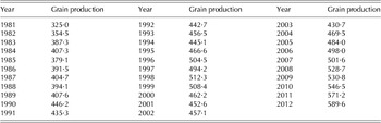
After the reform and adoption of the open door policy in 1978, grain production in China increased continuously with high growth rate for 6 years. After 1984, the annual grain output fluctuated around the level of c. 400 million tons (1996, 1998 and 1999 were exceptions, with output exceeding 500 million tons. The total output in 1996 reached 504·53 million tons thereby exceeding 500 million tons for the first time. However, in 2000, grain output began to decline dramatically and this situation continued for 4 years. As a result, the output in 2003 dropped to the level of a decade before. From 2004 to 2008, grain production rose continuously from 469·46 to 528·50 million tons, the highest peak in 30 years (NBS 2013).
The experimental data listed in Table 1 (NBS 2013) were used for model simulation, among which 32 data from 1981 to 2012 were adopted as the modelling and validating data. Since 32 data belonged to a small sample, the optimization grey model developed provided an appropriate approach because of its ability to use small samples for forecasting future grain production in China.
Grain production (million tons) in China from 1981 to 2012

GIM (1) model
The time sequence could be expressed as (Deng Reference Deng1982; Xie & Liu Reference Xie and Liu2009):
x (0)(1), x (0)(2),…, x (0)(n), where X (0)={x (0)(1), x (0)(2),…, x (0)(n)} was a raw data sequence, the sequence X (1)={x (1)(1), x (1)(2),…, x (1)(n)} was the first accumulated generation operation (1–AGO) sequence of X (0), and
 $$x^{(1)} (i) = \sum\limits_{k = 1}^i {x^{(0)} (k)}, \,i = 1,2, \ldots, n$$
The 1–AGO could be taken back to a discrete sequence as follows:
 $$x^{(0)} (i + {\rm 1}) = x^{({\rm 1})} (i + {\rm 1})-x^{({\rm 1})} (i)$$
Given the raw sequence {x (0)(i)} I=1,2,…,n, it could obtain the (1–AGO) {x (1)(k)}, then the GIM (1) model (Xiang Reference Xiang1997) could be expressed as the following differential equation:
 $$\displaystyle{{{\rm d}x^{(1)}} \over {{\rm d}i}} + a\displaystyle{{x^{(1)}} \over i} = b$$
The solution of Eqn (3) was
 $$x^{(1)} (i) = pi^{-{\rm a}} + qi$$
where
 $$p = x^{(1)} (1) - \displaystyle{b \over {1 + a}}$$
and
 $$q = \displaystyle{b \over {1 + a}}$$
Here, a, b, p and q were grey parameters. They could be obtained by the least squares method (LSM).
Denote â=[a,b]T, then
 $$\^a = \left[ {a,b} \right]^{\rm T} = \left[ {A^{\rm T} A} \right]^{-{\rm 1}} A^{\rm T} Y$$
where
 $$A = \left[ {\matrix{ { - \displaystyle{{x^{(1)} (i_2 )} \over {i_2}}} & 1 \cr { - \displaystyle{{x^{(1)} (i_3 )} \over {i_3}}} & 1 \cr { {\cdot} \cdot {\cdot}} & { {\cdot} \cdot {\cdot}} \cr { - \displaystyle{{x^{(1)} (i_n )} \over {i_n}}} & 1 \cr}} \right]$$
and
 $$Y = \left[ {\matrix{ {x^{(0)} (i_2 )} \cr {x^{(0)} (i_3 )} \cr { {\cdot} \cdot {\cdot}} \cr {x^{(0)} (i_n )} \cr}} \right]$$
So the values of a and b could be obtained. Then the grey parameters p and q were determined by LSM.
Suppose that
 $\mathop{r}\limits^\frown = \left[ {\,p,q} \right]^{\rm T}, $
p and q could be expressed as:
 $$\mathop{r}\limits^\frown = \left[ {\,p,q} \right]^{\rm T} = \left[ {B^{\rm T} B} \right]^{-{\rm 1}} B^{\rm T} Z$$
where
 $$ B = \left[ {\matrix{ {i_1^{ - {\rm a}}} & {i_2^{ - {\rm a}}} & { {\cdot} \cdot {\cdot}} & {i_n^{ - {\rm a}}} \cr {i_1} & {i_2} & { {\cdot} \cdot {\cdot}} & {i_n} \cr}} \right]^{\rm T} $$
and
 $$ Z = \left[ {x^{({\rm 1})} (i_{\rm 1} ),x^{({\rm 1})} (i_{\rm 2} ), \ldots, x^{({\rm 1})} (i_n )} \right]^{\rm T} $$
Finally, Eqn (4) could be determined.
GLPM (1) model
Similar to the GIM (1) model, GLPM (1) model (Liu & Yu Reference Liu and Yu2007) could be expressed as:
 $$ \displaystyle{{{\rm d}x^{(1)}} \over {{\rm d}i}} + a\displaystyle{{x^{(1)}} \over i} = b\displaystyle{{\ln i} \over i}$$
The solution to Eqn (3′) was:
 $$ x^{{\rm (1)}} (i) = ci^{-{\rm a}} + p\,{\rm ln}\, i + q$$
where
 $$ p = \displaystyle{b \over a}$$
and
 $$ q = \displaystyle{b \over {a^2}} $$
Similarly to GIM (1) model, the grey parameters a, b, c, p and q could be determined by LSM.
Let â=[a,b]T, then a and b could be expressed as:
 $$ \^a = \left[ {a,b} \right]^{\rm T} = \left[ {A^{\rm T} A} \right]^{-{\rm 1}} A^{\rm T} Y $$
where
 $$A = \left[ {\matrix{ { - \displaystyle{{x^{(1)} (i_2 )} \over {i_2}}} & {\displaystyle{{\ln i_2} \over {i_2}}} \cr { - \displaystyle{{x^{(1)} (i_3 )} \over {i_3}}} & {\displaystyle{{\ln i_3} \over {i_3}}} \cr { {\cdot} \cdot {\cdot}} & { {\cdot} \cdot {\cdot}} \cr { - \displaystyle{{x^{(1)} (i_n )} \over {i_n}}} & {\displaystyle{{\ln i_n} \over {i{}_n}}} \cr}} \right]$$
and
 $$Y = \left[ {\matrix{ {x^{(0)} (i_2 )} \cr {x^{(0)} (i_3 )} \cr { {\cdot} \cdot {\cdot}} \cr {x^{(0)} (i_n )} \cr}} \right]$$
Then using the method of LSM, the values of c, p and q were expressed as:
 $$\mathop{r}\limits^\frown = \left[ {c,p,q} \right]^{\rm T} = \left[ {B^{\rm T} B} \right]^{-{\rm 1}} {\rm} B^{\rm T} Z$$
where
 $$B = \left[ {\matrix{ {i_1^{ - {\rm a}}} & {\ln i_1} & 1 \cr {i_2^{ - {\rm a}}} & {\ln i_2} & 1 \cr { {\cdot} \cdot {\cdot}} & { {\cdot} \cdot {\cdot}} & { {\cdot} \cdot {\cdot}} \cr {i_n^{ - {\rm a}}} & {\ln i_n} & 1 \cr}} \right]$$
and
 $$Z = \left[ {\matrix{ {x^{(1)} (i_1 )} \cr {x^{(1)} (i_2 )} \cr { {\cdot} \cdot {\cdot}} \cr {x^{(1)} (i_n )} \cr}} \right]$$
Finally, Eqn (4′) could be determined.
GPPM (1) model
As a kind of derivative model of GM (1, 1) model, the GPPM (1) model (Xiang Reference Xiang1996), similar to GIM (1) model and GLPM (1) model, could be expressed as:
 $$\displaystyle{{{\rm d}x^{(1)}} \over {{\rm d}i}} + a\displaystyle{{x^{(1)}} \over i} = bi + \displaystyle{k \over i}$$
The solution to Eqn (3″) was:
 $$x^{({\rm 1})} (i) = ci^{-{\rm a}} + pi^{\rm 2} = q$$
where
 $$p = \displaystyle{b \over {2 + a}}$$
and
 $$q = \displaystyle{k \over a}$$
Like GIM (1) model and GLPM (1) model, the grey parameters a, b, k, c, p and q could be estimated by LSM. Let â=[a,b,k]T,
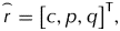 $\mathop{r}\limits^\frown = \left[ {c,p,q} \right]^{\rm T}, $
then one could have:
 $$\^a = \left[ {a,b,k} \right]^{\rm T} = \left[ {A^{\rm T} A} \right]^{-{\rm 1}} {\rm} A^{\rm T} Y$$
where
 $$A = \left[ {\matrix{ { - \displaystyle{{x^{(1)} (i_2 )} \over {i_2}}} & {i_2} & {\displaystyle{1 \over {i_2}}} \cr { - \displaystyle{{x^{(1)} (i_3 )} \over {i_3}}} & {i_3} & {\displaystyle{1 \over {i_3}}} \cr { {\cdot} \cdot {\cdot}} & { {\cdot} \cdot {\cdot}} & { {\cdot} \cdot {\cdot}} \cr { - \displaystyle{{x^{(1)} (i_n )} \over {i_n}}} & {i_n} & {\displaystyle{1 \over {i_n}}} \cr}} \right]$$
and
 $$Y = \left[ {\matrix{ {x^{(0)} (i_2 )} \cr {x^{(0)} (i_3 )} \cr { {\cdot} \cdot {\cdot}} \cr {x^{(0)} (i_n )} \cr}} \right]$$
In addition,
 $$\mathop{r}\limits^\frown = \left[ {c,p,q} \right]^{\rm T} = \left[ {B^{\rm T} B} \right]^{-{\rm 1}} {\rm} B^{\rm T} Z$$
and B and Z were represented as
 $$B = \left[ {\matrix{ {i_1^{ - {\rm a}}} & {i_1^2} & 1 \cr {i_2^{ - {\rm a}}} & {i_2^2} & 1 \cr { {\cdot} \cdot {\cdot}} & { {\cdot} \cdot {\cdot}} & { {\cdot} \cdot {\cdot}} \cr {i_n^{ - {\rm a}}} & {i_n^2} & 1 \cr}} \right]$$
and
 $$Z = \left[ {\matrix{ {x^{(1)} (i_1 )} \cr {x^{(1)} (i_2 )} \cr { {\cdot} \cdot {\cdot}} \cr {x^{(1)} (i_n )} \cr}} \right]$$
where i j=j(j=1,2,3,…,n) and x (0)(i) could be determined by Eqn (2).
Improved models based on the PSO algorithm
When the grey parameters were estimated by the LSM, an error existed in the calculation process. In order to improve prediction precision, PSO was applied to search for better grey parameters, in order to make the errors as small as possible.
Particle swarm optimization is an evolutionary computation technique. Being a kind of heuristic algorithm based on swarm intelligence, it originated from the simulation of simple social systems used to investigate the behaviour of feeding birds (Kennedy & Eberhart Reference Kennedy and Eberhart1995; Zou et al. Reference Zou, Fu, Yang and Zhang2006). In PSO, particles (individuals) representing a potential problem solution move through an n-dimensional search space. Each particle has a position vector (x i ), a velocity vector (v i ) and a fitness value decided by the objective function. From one iteration to another, the swarm renews itself by tracking two extreme values, termed Pbest and Gbest; Pbest means that each particle maintains a record of the position of its previous best performance in a vector, whereas Gbest equals the global best value, meaning that the particle took the entire population as its topological position (Huang & Dun Reference Huang and Dun2008). The velocity and position of a particle in the next step can be updated, respectively, by the following formula (Yang & Li Reference Yang and Li2004; Hao et al. Reference Hao, Huang and Yang2006; Qi et al. Reference Qi, Ma, Hu, Reffye and Cournède2010).
 $$\eqalign{v_i (k + {\rm 1}) = & v_i (k) + c_{\rm 1} rand_{\rm 1} ()(Pbest_i (k) - x_i (k)) \cr & + c_{\rm 2} rand_{\rm 2} ()(Gbest_i (k) - x_i (k))} $$
 $$x_i (k + {\rm 1}) = x_i (k) + v_i (k + {\rm 1})$$
where c 1 and c 2 were personal and social learning factors. Appropriate values of c 1 and c 2 could accelerate the conservation speed and did not fall easily into the local optimum. Uniform random numbers rand 1 and rand 2 were in the range of [0, 1] and Pbest i and Gbest i denoted the best previous position of particle i and the global position in the swarm, respectively. The velocity of every particle was restricted to the [–v max, v max] range in which v max was a predefined boundary value.
The grey parameters in the model could be estimated by LSM, but the error was significant. In order to minimize the error, PSO was applied to optimize the parameters. It is supposed that the estimated value of the original grey parameter was vector â and δ was a small perturbation in the range of [0, 1]. Then the estimated grey parameter could be reappraised by PSO in such a way that the small perturbation δ was added to the estimated parameter â, and it was reappraised in the range of [â−δ, â+δ], making the forecasting error as small as possible. What must be mentioned here was that the mean absolute percentage error (MAPE) defined as follows was employed to control the PSO processing:
 $${\rm MAPE} = \displaystyle{1 \over n}\sum\limits_{i = 1}^n {\left\vert {\displaystyle{{x^{(0)} (i) - \hat x^{(0)} (i)} \over {x^{(0)} (i)}} \times 100\%} \right\vert} $$
where x
(0)(i) and
 $\hat x^{(0)} (i)$
were the actual value and the predicted value, respectively.
Error evaluation criteria
Accuracy is an important index to measure the ability of forecasting methods (Yokuma & Armstrong Reference Yokuma and Armstrong1995; Hsu Reference Hsu2009; Li et al. Reference Li, Yeh and Chang2009). In order to evaluate the capability and accuracy of these three improved forecasting models, apart from the MAPE evaluation criterion defined in Eqn (15), the following five criteria were also employed to evaluate the prediction accuracy of the models related (He et al. Reference He, Hu, Chen, Suter, Li, Li, Yuan and Huang2010; Duan et al. Reference Duan, Yang, Bi, Chen, Luo and Liu2011): the root mean square error (RMSE), the standard error of prediction (SEP), the mean relative percentage error (MRPE) and the mean absolute error (MAE) were defined as follows:
 $${\rm RMSE} = \sqrt {\displaystyle{{\sum\limits_{i = 1}^n {(x^{(0)} (i) - \hat x^{\,(0)} (i))^2}} \over n}}$$
 $${\rm SEP} = \displaystyle{{100} \over {\bar X}}\sqrt {\displaystyle{{\sum\limits_{i = 1}^n {(\hat x^{\,(0)} (i) - x^{\left( 0 \right)} (i))^2}} \over n}} $$
 $${\rm MRPE} = \left[ {\displaystyle{1 \over n}\sum\limits_{i = 1}^n {\displaystyle{{x^{(0)} (i) - \hat x^{\,(0)} (i)} \over {x^{\,(0)} (i)}}}} \right] \times 100\% $$
 $${\rm MAE} = \displaystyle{1 \over n}\sum\limits_{i = 1}^n {\left\vert {x^{\,(0)} (i) - \hat x^{(0)} (i)} \right\vert} $$
where x
(0)(i) was the actual value,
 $\hat x^{\,(0)} (i)$
was the predicted value and
 $\bar X = \sum\nolimits_{i = 1}^n {x^{(0)} (i)/n} $
.
RESULTS
Forecasting results
The proposed new models, namely PSO–GIM (1), PSO–GPPM (1) and PSO–GLPM (1), were implemented along with the corresponding traditional models, namely GIM (1), GPPM (1) and GLPM (1), to simulate the grain production data from 1981 to 2012 and to forecast the grain production values from 2013 to 2022.
In the present paper, for comparison, the new proposed models were validated according to the following four tests, among which the first two tests were conducted based on original grain production data:
-
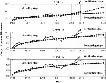
Test 1: The first 28 grain production data sets (from 1981 to 2008) were used for modelling and the other four (from 2009 to 2012) for verification.
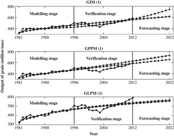
Test 2: The first 16 data sets (from 1981 to 1996) were used for modelling and the other 16 (from 1997 to 2012) for verification, i.e. half the data was used for modelling and half for verification.
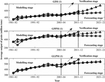
The remaining two tests were carried out based on the following pre-processed data: the data from every 2 years were grouped, i.e. the average grain production in 1981/82, 1983/84, etc. Hence, there were 16 data sets concerning the average production in 2 consecutive years. Then Tests 3 and 4 were designed as follows:
Test 3: The first 12 pre-processed data sets were used for modelling and the other four for verification.
Test 4: The first eight pre-processed data sets were used for modelling and the other eight for verification.
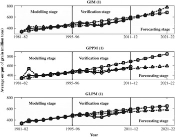
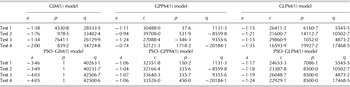
Parameters in the 1–AGO sequence {x (1)(k)} of the grain production obtained by the six models based on the grain production data from 1981 to 2012 are shown in Table 2. After the inverse 1–AGO process was conducted and expressed in Eqn (2), the forecasted grain output could be gained. The simulated/forecasted values obtained by each new model and its corresponding traditional model in modelling stages, verification stages and forecasting stages from Test 1 to Test 4 are shown in Figs 1 to 4, respectively.
Comparison among the actual (○) grain production values and the grain production values obtained by the original models (□) and the corresponding PSO optimized models (Δ) in Test 1.

Comparison among the actual (○) grain production values and the grain production values obtained by the original models (□) and the corresponding PSO optimized models (Δ) in Test 2.

Comparison among the actual (○) grain production values and the grain production values obtained by the original models (□) and the corresponding PSO optimized models (Δ) in Test 3.

Comparison among the actual (○) grain production values and the grain production values obtained by the original models (□) and the corresponding PSO optimized models (Δ) in Test 4.

Parameters in the 1–AGO sequences obtained by the six models

As observed from Figs 1 to 4, the first data obtained by the six models in the modelling stage were all equal to the corresponding actual value. Among the three PSO optimized models, i.e. PSO–GIM (1), PSO–GPPM (1) and PSO–GLPM (1), the curves obtained by the PSO–GLPM (1) model were the closest to the corresponding un-optimized model, no matter how much the data used for modelling and verification changed. In addition, among the four tests, no more than 28 data sets were used to set up the grey forecasting models, whereas for most of the traditional forecasting approaches, a complete database was needed to build the essential mathematical models. It is very clear that all the grey forecasting models in the present article could predict the future data of grain production with limited data.
Then five evaluation criteria were applied to compare the accuracy and stability of the forecasting approaches, namely MAPE, RMSE, SEP, MRPE and MAE. The comparison results for the six forecasting methods are shown in Table 3.
Forecasting performance of the six models for the grain production example

The error values in the verification stage were the most important information source to determine whether the PSO-based models were really better than the corresponding un-optimized ones, since the modelling stage was just to set up the model and the corresponding actual grain production values in the forecasting stage were unknown. For the verification stages, it could be judged from the relevant statistical indices that all PSO-based models performed better than the corresponding traditional ones.
The MAPE values for the three new models in verification stages were smaller than those of the corresponding traditional ones. In the case of the other indices, RMSE, SEP, MRPE and MAE, the performances of the new models were superior to those of the corresponding original ones except for the PSO–GLPM (1) model, which provided larger RMSE, SEP and MAE values than the GLPM (1) method in Test 2. However, in most cases, the PSO–GLPM (1) model still outperformed the GLPM (1) method. These data proved that PSO–GIM (1), PSO–GPPM (1) and PSO–GLPM (1) were adequate with regard to both accuracy and stability. Thus, the PSO-optimized grey parameters could mitigate the drawbacks of original models, and the new models using PSO to optimize the grey parameters were more accurate than the corresponding traditional models using the least square method. Although PSO-optimized models failed to perform in modelling stages compared with the original ones, their performance in verification stages were excellent. Since those models with better capability in verification stages were really needed and would be applied to subsequent forecasting, therefore, the new models possessed better performance than the traditional ones.
In addition, the MAPE, SEP, MRPE and RMSE values indicated that the proposed approach, PSO–GIM (1), outperformed the five other methods. In addition, as compared to Test 4, the six models always provided smaller MAPE values than they did in the verification stages of Test 3. This could be explained as follows: with the increase of the data in the modelling stage, more information was acquired and thus the model will probably be set up more accurately. However, the same situation did not appear in Test 1, even though it had more modelling data than Test 2. However, no matter in which tests, the application of PSO in the parameter optimization of GIM (1), GPPM (1) and GLPM (1) made the MAPE values decrease greatly, proving that the forecasting ability of PSO optimal models were stronger than those of the corresponding traditional ones.
DISCUSSION
Accurate grain production forecasting based on historical data is very challenging due to the influence of many factors, for instance agricultural techniques, weather, land use change, etc Traditional approaches such as the ARIMA model and the artificial neural network model can merely provide a rough estimation for a small sample size, and their prediction accuracy can only be guaranteed under the conditions of a large sample size. In order to improve the prediction accuracy, the present paper proposed three new models for grain production forecasting by combining PSO with the traditional GIM (1) model, GPPM (1) model and GLPM (1) model. The experimental results indicated that the new models were superior to the traditional models.
One of the contributions of the present study is to modify the algorithm of GIM (1), GPPM (1) and GLPM (1) with the PSO technique. Grey forecasting models have been adopted successfully in various fields since they were first proposed; however, they are unsatisfactory in the aspect of precision when using more random data, especially in predicting the development of a complex or instable system, the performance of adopting grey models would be rather limited for the sake of rapidly changing system development rate resulting from various interactive factors (Lin & Lee Reference Lin and Lee2007). But the optimized models proposed in the present paper can deal with the random time series more effectively and more accurately, and they are high-precision forecasting models for grain production in China.
The empirical results reveal that the optimized grey prediction models in the present paper can be applied to China's grain production forecasts very well. The three new models proposed, namely PSO–GIM (1), PSO–GLPM (1) and PSO–GPPM (1), are simple and valid. The much higher prediction accuracy of PSO optimized grey forecasting models than that of the original grey models demonstrates that the PSO technique could be regarded as a good tool for grey parameters optimization and accuracy improvement.
The work was supported by the National Natural Science Foundation of China (Grant no. 71171102).