For over a decade now our thinking on the political economy of the welfare state has focused on labor market risks and social insurance policy (Hall and Soskice Reference Hall and Soskice.2001; Iversen and Soskice Reference Iversen and Soskice2001; Moene and Wallerstein Reference Moene and Wallerstein2001; Moene and Wallerstein Reference Moene and Wallerstein2003). Citizens’ preferences over various social insurance policies (unemployment, disability, retirement, etc.) are held to be a function of the economic risks they face. Simultaneously, existing levels of social insurance affect workers’ willingness to acquire particular types of skills that may be more prone to obsolescence.
In focusing on individuals alone, this literature pays little attention to the fact that most economic decisions, especially regarding risk and insurance, are made at the household level.Footnote 1 Households in advanced economies of the Organization for Economic Cooperation and Development (OECD) typically rely on one or two individuals who earn the majority of household income through participation in the formal labor market. These earners are mutually dependent on one another but they may also have others (children, elders, or disabled persons) who also depend on them. In single-earner households, there may be a second adult who refrains from entering into the labor market in order to provide household services. These individuals depend directly on their partners for money income, yet they often care for other dependents and vote.
Major studies of public support for social insurance policies have failed to account for marital status, head of household, or the presence of children (or other dependents) in their models of public opinion (Iversen and Soskice Reference Iversen and Soskice2001; Scheve and Stasavage Reference Scheve and Stasavage2006; Rehm Reference Rehm2009; Rehm Reference Rehm2011; Nickelsburg and Timmons Reference Nickelsburg and Timmons2012). This omission is particularly worrying given the growing behavioral economics literature examining how major life events, including marriage, child bearing, and aging can affect people’s attitudes toward risky choices (Sundn and Surette Reference Sundn and Surette1998; Bellante and Green Reference Bellante and Green2004; Drewianka Reference Drewianka2008; Bertocchi, Brunetti and Torricelli Reference Bertocchi, Brunetti and Torricelli2010). The joint effect of labor market participation and marriage on risk acceptance is most pronounced among women (Sundn and Surette Reference Sundn and Surette1998; Bertocchi, Brunetti and Torricelli Reference Bertocchi, Brunetti and Torricelli2010).
In this paper, we take steps toward a better understanding of how these household interactions affect preferences for the cornerstone of the welfare state—insurance against job loss. We use a stylized laboratory setting to focus on a generic household relationship: dependency, either mutual or asymmetric. Our findings indicate that the willingness to vote in favor of a social insurance policy is responsive to unemployment risk and one’s asymmetric dependence on another for income. We then show that our lab findings are also visible in survey data.
The Political Economy of Social Insurance
Redistribution and Insurance
There is a large body of theoretical and empirical work looking at the demand for both direct income redistribution and socialized insurance.Footnote 2 Purely redistributive policies involve taxing a population (or some subset) and then distributing proceeds such that some are necessarily net beneficiaries and others are necessarily net contributors. Under canonical models of redistribution (e.g., Meltzer and Richard Reference Meltzer and Richard1981), the tax and distribution rules are known and agents anticipate whether they will be net beneficiaries, inducing preferences over tax rates and spending levels. Social insurance policies, on the other hand, are policies that mandate contributions in order to insure against specific risks. At the time of tax assessment agents do not know whether they will be (net) beneficiaries; there is some fundamental uncertainty against which the program is meant to insure. In canonical models, contributions to the social insurance program are universal.
Scholars make an analytic distinction between simple redistribution and social insurance. In the real-world economic risk exposure is often inversely related to income or wealth. Factors affecting demand for insurance and redistribution intertwine in complicated ways. Separating insurance effects (desire to insure against bad states) from redistributive concerns (desire to equalize relative outcomes across individuals or groups) is a key technical challenge. Most of the experimental literature examines voting in groups over explicitly redistributive policies (Rutstrom and Williams Reference Rutstrom and Williams2000; Cabrales, Nagel and RodrguezMora Reference Cabrales, Nagel and RodrguezMora2012; Agranov and Palfrey Reference Agranov and Palfrey2014).Footnote 3 Few studies that examine social insurance (Esarey, Salmon and Barrilleaux Reference Esarey, Salmon and Barrilleaux2011a; Barber, Beramendi and Wibbels Reference Barber, Beramendi and Wibbels2013) approach the insurance versus redistribution issue in different ways. In this study, we use our experimental design to explicitly avoid any concern with redistribution, both within and across “households,” thereby isolating the income dependency and the insurance concerns that motivate this paper.
Household Economics and Gendered Voting
The voluminous literature on the economics of the household largely examines consumption, intrahousehold resource allocation, and labor supply decisions (Lundberg and Pollak Reference Lundberg and Pollak1996; Fortin and Lacroix Reference Fortin and Lacroix1997; Gray Reference Gray1998; Ashraf Reference Ashraf2009; Hotz, Peet and Thomas Reference Hotz, Peet and Thomas2013). In this literature, there is a division among those who view the household as a unitary actor and those taking a more complicated view of intrahousehold relations and decisionmaking.Footnote 4 For political economists there is good reason to adopt the latter view.Footnote 5 This literature, however, largely ignores political economy issues.
In political science there is a parallel literature on gender differences in voting, based on an observation that women in rich countries tend to identify more with and vote for left-leaning parties. Edlund and Pande (Reference Edlund and Pande2002), for instance, find evidence that women have become more left-leaning in their voting behavior, which the authors correlate with lower marriage rates and higher divorce rates. However, in the American context, Burden (Reference Burden2008) finds that this partisan gender gap shrinks markedly when survey questions prime “feelings” rather than “thoughts.” In addition, Finseraas, Jakobsson and Kotsadam (Reference Finseraas, Jakobsson and Kotsadam2012) use a Norwegian data set to evaluate the findings of Edlund and Pande (Reference Edlund and Pande2002). They find that gender differences are largely due to more left-leaning voting by single women, with no robust effect of divorce risk or labor force participation.
Iversen and Rosenbluth (Reference Iversen and Rosenbluth2010) provide the most articulated link between the household economics and gender voting gap literatures. In their telling, household economic decisions are the result of bargaining between partners. Should the partnership dissolve each partner faces different outside options; the quality of each partner’s outside option determines bargaining leverage inside the partnership. External macroeconomic structures, in turn, determine the relative value of men’s versus women’s labor in the labor market, which then determine the outside option for women. Where women have poor outside options, policies “that favor the male breadwinner are therefore also policies that benefit women who are more or less completely dependent on their husbands” (Iversen and Rosenbluth Reference Iversen and Rosenbluth2010, 115). But there are two wrinkles here when it comes to social insurance. First, according to Iversen and Rosenbluth, women in the United States (where we gather our data) have relatively good outside options due to the “general skills” nature of the American political economy. Second, the expected gender-based differences in political preferences arise around issues of public employment and child care. “[M]any of the other spending questions—about pensions, unemployment, and so on—are not clearly related to gender conflict” (Iversen and Rosenbluth Reference Iversen and Rosenbluth2010, 119). So while we may see gender differences in partisan support, it is not clear they will be visible in levels of support for specific welfare policies.
In our experiments, we bracket concerns with intrahousehold bargaining in order to focus directly on the relationship between dependency structure and political preferences. Partnerships are induced randomly and there is no ability to dissolve them. The within-partnership division of income is fixed exogenously as are the labor market opportunities available to subjects. We ask whether there is evidence of a “dependency effect” even in the absence of or in addition to more complicated intrahousehold relations.
Dependency, Risk, and Implications for Social Insurance Demand
People bound together in dependency relationships might view income insurance differently than those who are not, but the directionality of this relationship is not obvious. A variety of other regarding payoff functions have been developed and evaluated in the theoretical and empirical economics literatures (Rabin Reference Rabin1993; Fehr and Schmidt Reference Fehr and Schmidt1999; Bolton and Ockenfels Reference Bolton and Ockenfels2000; Charness and Rabin Reference Charness and Rabin2002; Falk and Fischbacher Reference Falk and Fischbacher2006). While these models generate richer predictions about cooperative behavior and envy, none readily admits a role for a dependency effect, especially an asymmetric one.
Psychologists and marketing researchers have explored household dependency relations. Recent work from consumer research theorizes that dependency relationships may in fact change individuals’ preferences, a stark departure from the intrahousehold bargaining research, which assumes family members with fixed, stable preferences. Simpson, Griskevicius and Rothman (Reference Simpson, Griskevicius and Rothman2012) develop an informal model of dyadic decisionmaking in which each member of a household has preferences and attitudes that affect the attitudes and preferences of their partner (see also Bagozzi Reference Bagozzi2012; Gorlin and Dhar Reference Gorlin and Dhar2012). Research in regulatory focus theory (Higgins Reference Higgins1998; Lee, Aaker and Gardner Reference Lee, Aaker and Gardner2000; Zhou and Pham Reference Zhou and Pham2004) finds that an interdependent outlook shifts an individual’s focus from promotion goals to prevention goals. Also in this field, Hamilton and Biehal (Reference Hamilton and Biehal2005) find that making dependency salient leads to loss-minimizing decisions consistent with increased risk aversion. However, there is evidence that this increased loss sensitivity may be more nuanced: Mandel (Reference Mandel2003) finds that someone with an interdependent focus may engage in more financially risk-seeking behavior if “social risk”—the risk of causing disappointment or disapproval—is salient.
In a closely related area, scholars examine how risk preferences differ between individuals and households, finding that decisions made jointly are generally more risk averse than those made by individuals (Bone, Hey and Suckling Reference Bone, Hey and Suckling1999; Bateman and Munro Reference Bateman and Munro2005; de Palma, Picard and Ziegelmeyer Reference de Palma, Picard and Ziegelmeyer2011; Abdellaoui, I’Haridon and Paraschiv Reference Abdellaoui, I’Haridon and Paraschiv2013; Carlsson et al. Reference Carlsson, Martinsson, Qin and Sutter2013; Munro, Bateman and McNally Reference Munro, Bateman and McNally2013; Braaten and Martinsson Reference Braaten and Martinsson2015). Several of these studies involve real-life couples engaged in abstract joint decisions over risky lotteries. Clarke and Kalani (Reference Clarke and Kalani2011) design a framed field experiment to study demographic effects on take-up of microinsurance (such as rainfall and other index insurance) among residents in rural Ethiopia. Though household structure is not focal in their analyses, they find a significant link between measured household risk aversion and enrollment in microinsurance. However, the voting decisions that interest us are not in fact joint decisions, even if they are correlated within households. Findings on risk tolerance within couples may translate to voting for social insurance programs, but the direct connection has not yet been made.
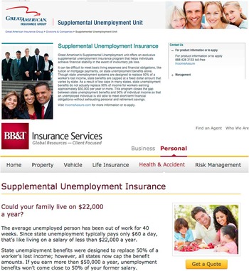
For their part, marketers of private insurance and other financial products often emphasize dependency relationships in their advertisements, as depicted in Figure 1.Footnote 6 Hopper (Reference Hopper1995) points out that families, not individuals, are the predominant purchasers of financial services and investment products. Marketing messages should therefore target both members of a household as well as the connection between members. Further research into the determinants of life insurance purchases suggests family dynamics play a key role (Anderson and Nevin Reference Anderson and Nevin1975; Ferber and Lee Reference Ferber and Lee1980; Goldsmith Reference Goldsmith1983; Zietz Reference Zietz2003).
Two examples of the marketing of private sector unemployment insurance in the United States (Accessed 1 April 2015)

Clearly, dependency relationships are important for joint decisions, especially insurance purchasing. There is some evidence that dependency status may, in fact, affect individual preferences. But all of this research emphasizes mutual or symmetric dependency, in contrast to the political economy of the household literature with its emphasis on differential outside options and asymmetric dependency. Much of the literature looks at joint economic decisions with very little discussion of political preferences. And voting decisions are, ultimately, individual-level choices, not joint ones. Existing bodies of theory provide minimal guidance on what to expect. We therefore view dependency effects on political preferences, especially for welfare state policies, as an overlooked area of research. The existence, directionality, and symmetry of such effects are empirical questions.
Expectations
Existing work across several disciplines suggests that dependency should “matter.” Isolating these relationships in an observational setting would be impossible, so we turn to the lab. In the experiment detailed in the next section, we manipulate the two key variables that emerge from the discussion above: labor market risk and dependency status. A key innovation of this study is an explicit consideration of asymmetric dependency.
We treat single subjects with no household ties as the “control” condition, representing the setup assumed in most extant models of social insurance. We examine whether subjects are sensitive to increased labor market risk, expecting subjects in high-risk treatments to vote for insurance at higher rates than those at lower risk (holding fixed insurance contributions). Second, we examine whether dependency matters. To achieve this, we construct three conditions. The first has subjects on their own, the “control” condition just mentioned. The second and third embed subjects in randomly constructed pairs. In one of these paired treatments both subjects are able to earn income and experience unemployment; we refer to this as the “paired, dual-earner” treatment. In the second paired treatment only one member of the pair (randomly determined) can earn (or suffer unemployment), while the other simply votes and shares in the earner’s income. We call this the “paired, single-earner” condition. If dependency matters then, conditioning on risk, we should see a difference in voting for social insurance between those paired off and those on their own. We compare the subjects in the paired, single-earner treatment with those on their own to explore whether there is any asymmetry in the dependency effect, that is, whether subjects factor in their partner’s vulnerability (if the “breadwinner” is more supportive of insurance) or they are more sensitive to risk when they, themselves, are unable to work for a wage (if the “homemaker” is more supportive of insurance).
Our key outcome of interest is the subjects’ voting behavior over social insurance policies. In the Supplementary Appendix C (online), we briefly discuss subjects’ effort levels in the experiment as a function of risk and dependency. We do this to show the extent of subject learning within experimental sessions and document that labor supply (as measured by task effort) does not differ significantly by experimental treatment.
The Lab Experiment
Experimental Design
We conducted experimental sessions at the University of Wisconsin BRITE lab and the xs/fs lab at Florida State University (FSU). Wisconsin subjects were recruited from large introductory courses and were told they would be participating in a political behavior research study that would last under two hours and pay roughly $20–30, including a fixed show-up fee. Recruiting at Florida State was done through Online Recruitment System for Economic Experiments (ORSEE) (Greiner Reference Greiner2015). All sessions in both locations were conducted using computer terminals separated by privacy dividers. The experimental software was implemented in zTree (Fischbacher Reference Fischbacher2007). Once all subjects had signed a consent form, instructions were distributed and read aloud, allowing for any questions to be answered publicly.
Subjects in each Wisconsin session were divided into groups of 8–12, with one or two groups in each session.Footnote 7 Sessions at Florida State divided 24 subjects into three groups of eight. Randomization and treatment assignment occurred at the session level.
Each session had two stages. The first stage consisted of ten production rounds in which the subjects earned money by completing an identical task. The second stage consisted of six guaranteed rounds after which we implemented a random stopping rule so that subjects had a 75 percent chance of seeing an additional round. In expectation subjects played a total of 20 rounds. The maximum number of rounds is 29 and minimum is 17 with an average of 22.
In each production round, subjects worked at a real-effort “slider” task (Gill and Prowse Reference Gill and Prowse2011; Gill and Prowse Reference Gill and Prowse2012). In this task, subjects see 48 “slider bars” scattered on the screen (see Figures in Supplementary Appendix A (online)) with a peg positioned at the left-most edge of each slider. Subjects used their mouse to drag the peg to the exact center of each slider, successfully completing the item when the number to the right of the slider read “50.” All subjects were given a 2-minute practice round to familiarize themselves with the slider task before round one. Subjects were paid a 120 ECU (experimental currency unit) fixed “wage” per round in addition to a 10 ECU “commission” per completed slider, with earnings accumulating over all rounds of the experiment.Footnote 8 The fixed wage and commission rates were chosen so that the fixed wage will equal approximately one-third of the expected per-round compensation, based on past experience with the sliders task.Footnote 9 In other words, we expect the piece rate earning to be about double the base wage.
We have two experimental manipulations: unemployment risk (high or low) and dependency status (single; paired, single earner; and paired, two earner). The dependency manipulation is meant to simulate, abstractly, various ways in which households might interact with the labor market. In the “single-earner-only” treatment subjects were not paired with anyone else and their payoffs depended only on their own actions and the random parameters of the experiment. In the “paired, dual-earner” treatment subjects were randomly assigned a partner. Both members of the pair were able to work at the slider task during production rounds as just described. Each member of the pair is independently subject to the same unemployment risk. In the “paired, single-earner” treatment subjects were randomly assigned a partner. At the beginning of the first stage, partners were randomly assigned a role—active or passive—such that each pair had one of each type. The active participant (corresponding to the notion of breadwinner) was able to work at the task, as described above, while the passive participant (i.e., the homemaker) was unable to work at the task during that stage. At the beginning of stage II, the participants switched roles.Footnote 10 In both the paired treatments subjects’ earnings were split equally between the matched subjects.Footnote 11 Subject pairs remain constant for all rounds in each stage.
We note immediately that our pairing protocol is quite weak. Pairing is anonymous, subjects are unable to communicate with one another, and there was no other intervention designed to increase the partner “bond.” We view our experiment as a difficult test for any dependency effect, as non-findings may be attributable to an insufficient bond between subjects. We also note that our paired, single-earner condition is not an instance of one partner simply having a weak “outside option” as partnerships cannot dissolve and the income sharing rule is fixed in our experiment.
We explore two different risk levels to see whether subjects are reacting to risk as we would expect and to ensure that we have some subjects who experience several rounds of “unemployment.” In each production round, there was a probability, q, that a subject would become “unemployed,” that is, be forced to sit out for a production round and forgo earnings. The value of p is constant for an entire experimental session and common for subjects within a session. For the low-risk treatments, q=0.05, approximately the American unemployment rate under tight labor market conditions. For the high-risk treatments, we set q =0.25, approximately equal to what we are currently witnessing in the depressed parts of Europe. All subjects were told the value of p for their session. We also explained that unemployment risk is independent across subjects and that each subjects’ unemployment risk is independent of their task performance and that of any other subject. As part of the comprehension quiz subjects were asked to state the unemployment risk for their session; the session was not allowed to proceed until all subjects answered this question correctly.
Before each stage subjects were presented with the opportunity to vote over a social insurance policy designed to partially insure participants against income losses from unemployment. Unlike other experimental studies focusing on the redistributive aspects of social insurance (Esarey, Salmon and Barrilleaux Reference Esarey, Salmon and Barrilleaux2011a; Barber, Beramendi and Wibbels Reference Barber, Beramendi and Wibbels2013), we take the policy proposal as exogenous.Footnote 12 Specifically, participants voted for either “option A” in which no insurance was provided and no taxes were levied or “option B” in which unemployed participants are guaranteed 120 ECU for that round, while all working participants contribute 7 ECU to an insurance fund. To explicitly avoid any redistributive consequences we do not require the budget to balance, that is, expenditures for insurance payments could exceed subjects’ contributions or there could be a surplus. Any deficit or surplus disappears at the end of the experiment; subjects are informed of all this.
The group decision is taken by majority vote. All subjects are able to vote, including the passive subjects in the paired, single-earner treatment. Voting is compulsory and ties are broken by random draw. Subjects were shown the adopted policy and the number of votes for and against.
Note that the 7 ECU insurance contribution, constant across both risk treatments, was derived as the value that would lead the insurance budget to balance in expectation under the low-risk condition, assuming an average slider score of 26.Footnote 13 This contribution is far less than the amount required to balance the budget under the high-risk condition. If subjects understand the situation then they should certainly vote in favor of insurance in the high-risk setting as their premiums are, in effect, massively subsidized. The decision is more ambiguous in the low-risk treatment.
The first vote takes place before subjects learn their employment status and, in the paired, single-earner treatment, their role. The second vote takes place after the completion of round ten. Among the subjects in the paired, single-earner treatment, none had prior experience for the first vote but for the second vote, half had been active during stage I and the other half passive. Importantly, neither group knew what its status would be for stage II at the time of the vote. Subjects in this treatment condition cast their second vote before they were told their role (active or passive) for the stage II rounds.
We emphasize that our protocol explicitly excludes redistributive concerns (whether from richer to poorer or more productive to less so) embedded in many real-world social insurance programs as well as the experimental (Esarey, Salmon and Barrilleaux 2011Reference Esarey, Salmon and Barrilleauxa; Barber, Beramendi and Wibbels Reference Barber, Beramendi and Wibbels2013) and observational (Iversen and Soskice Reference Iversen and Soskice2001; Scheve and Stasavage Reference Scheve and Stasavage2006; Rehm Reference Rehm2009; Rehm Reference Rehm2011; Nickelsburg and Timmons Reference Nickelsburg and Timmons2012) studies that look at them. Other studies ask respondents to enter a preferred tax rate and then pay subjects as a proportion of group income, implying distributive consequences to insurance. In our setup, we have subjects vote before they fully realize their level of productivity. We also set contribution rates exogenously. But most importantly, we do not force the budget to balance breaking any direct dependence between payments to subjects. It is now possible for everyone to be a net beneficiary or a net contributor; a payment to one does not come out of the pocket of another.
At the beginning of each production round, all subjects were informed whether they would participate in the task that round or sit out. Participating subjects then had 2 minutes to work at the sliders task, while those sitting out saw a blank screen. At the end of each production round subjects in the single-earner treatment saw whether they participated in the task, their performance in completed sliders, and their payoff in ECU. They also saw this information for prior rounds. Subjects in the paired treatments saw this information for themselves as well as their partner. Figure 3 in Supplementary Appendix A (online) displays a screen shot of the feedback given to participants.
After the final round, all participants completed a questionnaire. All subjects were paid privately, in cash, at the conclusion of the session.
We conducted 15 experimental sessions composed of 35 unique groups for a total of 282 valid participants. Details on the number of subjects in each treatment from each location are presented Supplementary Appendix B (online).
Experimental Results
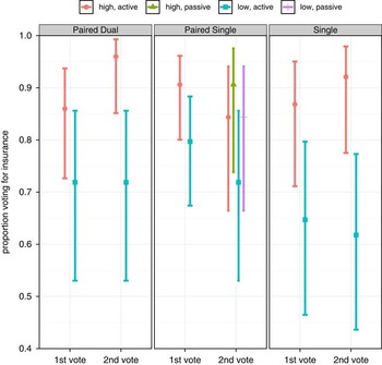
Figure 2 displays the basic results for the voting experiment. Each panel represents one of the different dependency treatments, while the colors of the bars depict risk levels and roles (for the paired, single-earner treatment). The points represent the proportion of subjects casting votes in favor of the insurance scheme, with associated 95 percent confidence intervals. Tables reporting numerical versions of these results along with sample sizes are presented in Supplementary Appendix B (online). There are three things to note: the high levels of support for insurance; the responsiveness to risk; and the asymmetric dependency effect.
Ex ante and mid-session voting for social insurance by dependency treatment, unemployment risk level (low risk=5 percent; high risk=25 percent), and stage I role Note: Subjects in the paired, single treatment did not know their role for stage I at the time of casting the first vote nor did they know their roles for stage II at the time of casting the second vote

First, regardless of risk or dependency considerations, subjects voted for insurance by large margins.Footnote 14 There were only two groups—both in the same low-risk dual-earner session—in which a majority of the subjects voted against insurance. While unsurprising in the high-risk treatments, the strong support for insurance under low risk is noteworthy: under low risk the price for insurance slightly exceeds both the amount needed to balance the budget and the expected individual benefit for any player.Footnote 15 The initial support for insurance in the ex ante vote might be attributed to subjects’ lack of familiarity with the slider task. Support for insurance did weaken in the second vote in the low-risk treatments, at least in the paired single, active earners, and single-earner dependency conditions. But this weakening of support was modest and not enough to switch the group decisions in any case. Subjects appear notably risk averse in this experiment.
Second, as expected, we recovered a strong sensitivity to risk. Across all three dependency conditions, subjects in the high-risk treatments were significantly more likely than those in the low-risk analogue to vote for insurance at the first opportunity. In the single-earner and paired, dual-earner treatments, these gaps grew between the first and second votes. Averaging across all dependency conditions the difference in pro-insurance voting proportions between high and low risk was 14 percentage points in the first vote (χ 2=9.5, p=0.002). This gap grew to 19 percentage points by the second vote (χ 2=17.9, p=0), a large number all the more remarkable given the high overall levels of support for insurance described above. Furthermore, changes in support for insurance from the first to the second vote responded differently in the two risk treatments. Among the single- and paired, dual-earner subjects, support increased in the high-risk condition but stayed about flat in the low-risk conditions although none of these differences achieve statistical significance at p≤0.05.
Third, we find weak evidence for the hypothesis that simple dependency status per se affects willingness to support insurance policies. In the high-risk setting, we see voting for insurance at similarly high rates across all dependency treatments; these rates are sufficiently close that we cannot distinguish among any of them statistically. In the low-risk condition, respondents in the paired treatments were marginally more supportive of insurance than subjects without dependents, but this difference was not significant.Footnote 16 But in the low-risk setting, we see clear evidence that subjects who had been the passive member of a single-earner partnership during stage I were substantially more likely to cast votes for insurance at the second opportunity. The passive member of single-earner partnerships voted for insurance at the highest rates, 12 percentage points higher than subjects in the other paired treatments and 22 percentage points higher (χ 2=4.3, p=0.04) than subjects with no experimentally induced dependency relationships. Subjects who were in the passive position in a partnership were, by the second vote, more likely to vote in favor of insurance than those in the any of the other dependency conditions, at least in the low-risk treatment.
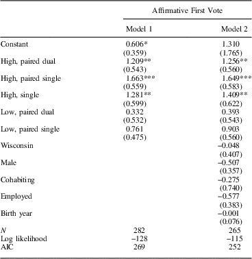
Regression analysis lets us examine these results more precisely. Table 1 displays logistic regression estimates for subjects’ first votes for insurance. We fit two models here. Model 1 includes only indicators for the randomly assigned dependency and risk treatments; the individual earner, low-risk treatment is the reference category. The second model also conditions on subjects’ gender, age, lab site, whether the subject is employed in the “real world,” and whether the subject is cohabiting with a spouse or domestic partner in addition to the experimental treatments. Including these additional covariates causes us to lose 17 observations due to non-response on the questionnaire.
Logistic Regression Parameter Estimates for First Vote on Social Insurance

Note: The single-earner, low-risk treatment is the reference category.
AIC=Akaike information criterion.
***p<0.01, **p<0.05, *p<0.1.
The regression results mirror those depicted for the first vote in Figure 2: subjects are responsive to risk but little else seems to matter. Demographic covariates have no predictive power in the first vote.
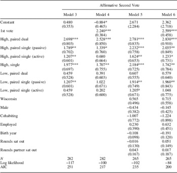
Table 2 displays estimates from four logistic regression models on the second vote for social insurance. Model 3 includes only experimental variables, while model 5 includes the additional covariates of gender, age, lab site, employment, and domestic status as well as the subjects’ experiences during the first stage: the number of rounds in which the subject was forced to sit out and the number of rounds the subject’s partner sat out. Models 4 and 6 also condition on subjects’ initial votes.Footnote 17
Logistic Regression Parameter Estimates for the Second Vote on Social Insurance

Note: The single-earner, low-risk treatment is the reference category.
AIC=Akaike information criterion.
***p<0.01, **p<0.05, *p<0.1.
By the second vote several patterns emerge. Unsurprisingly, we continue to see the strong and robust risk effect across all model specifications. The rate of pro-insurance voting in the high-risk setting is so elevated that subject behavior across dependency treatments is indistinguishable.
More interesting is our ability to discern a significant asymmetric dependency effect under lower risk at the second vote, taken after subjects have some experience with the task and their roles.Footnote 18 Subjects in the passive role of the paired, single-earner treatment, that is, those who have just had the experience of being dependent on someone else, are significantly more likely to support insurance than otherwise similar subjects able to earn on their own. This finding is robust to the inclusion of a variety of covariates, including the first vote. Again, we find no added value from including covariates. This is particularly important as we are conditioning on both own and partner’s experience with unemployment (number of rounds sitting out). The actual experience of unemployment has no discernible effect on the likelihood of pro-insurance voting once we know the risk of unemployment and dependency relationships. This gives us more confidence that our findings can be interpreted as a dependency effect rather than simply the result of having sat out ten consecutive rounds.
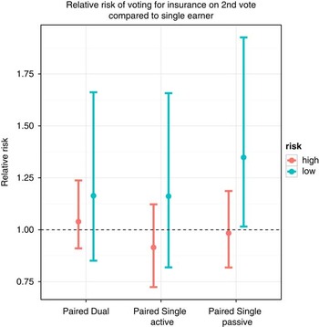
The model has a series of interesting comparisons that are difficult to extract from the table. To better interpret findings we use Model 3 to generate expected “relative risks” of voting for insurance at the second vote. Specifically, we divide the predicted probability of a pro-insurance vote for subjects in a particular treatment by the predicted probability of a pro-insurance vote for a single earner of the same unemployment risk level.Footnote 19 A value of unity indicates that the subjects in the two conditions are equally likely to vote for insurance. Relative risks greater than one indicate percent by which a subject’s probability of supporting insurance exceeds that for a single earner facing the same unemployment rate. The figure shows that passive subjects in the single earner, low unemployment condition are, on average, 35 percent more likely to vote for insurance than a similar single earner. We are unable to distinguish any of the other dependency/risk combinations from their individual earner counterparts (Figure 3).
Relative risk of voting for social insurance at the second vote comparing subjects with those in the single-earner condition at the same unemployment risk level Note: points are median estimates from 1000 simulations and vertical bars are 95 percent confidence intervals. Estimates derived from model 3

One may question whether a single-earner subject is the appropriate baseline for comparison. For example, why is the asymmetric dependency effect discernible only when we compare the passive member of a single-earner partnership with a solitary subject but not when we compare her with the active member of a single-earner partnership? We believe that the single earner provides the appropriate baseline for two reasons. First, the existing theoretical and empirical literature motivating this study takes the hypothetical single individual as the prototype. Second, we have no ex ante reason to believe that the appropriate way to measure treatment effects is within a particular dependency treatment. Rather, we view the single earner as the benchmark against which to measure possible deviations among both the active and passive halves of single-earner partnerships. From a practical standpoint, the lack of a significant difference between the passive and active members of a single-earner partnership (or between active partners and single earners) could arise for a variety of reasons, including weaker effects requiring bigger samples, an insufficiently strong partner bond in our experimental setting, or simply sampling variability. Appropriately evaluating these possibilities is an opening for additional research.
The laboratory experiment, even with its stylized setting and with no attempt at inducing any connection between subjects beyond anonymously sharing earnings, managed to uncover a significant asymmetric dependency effect. Before having any real experience with the task, subjects only displayed sensitivity to the stated risks of unemployment. After having some experience with the task and their roles, however, subjects who were randomly made dependent on the earnings and employment of a partner but who were unable to earn on their own were more supportive of insurance; subjects who were made jointly dependent but where both could earn showed no such difference in behavior.
Evidence from Survey Data
The lab findings allowed us to demonstrate a dependency effect even when partnering is exogenous, the redistributive effects of social insurance are removed, and real-world household politics are assumed away. But we also use an undergraduate subject pool who are less exposed to adult household relationships and may be more selfish and narrowly “rational” (Belot, Duch and Miller Reference Belot, Duch and Miller2015). So how general are our findings? Are similar correlations visible in observational settings?
To answer to these questions, we turn to the General Social Survey (GSS). In several years (1985, 1990, 1996, and 2000), the GSS asked respondents their attitudes about government-provided benefits for the unemployed.Footnote 20 Critically, the GSS, alone among major social science surveys, also includes questions asking about the respondent’s own labor force participation as well as that of their spouse (if any). This allows us to classify respondents into six mutually exclusive categories, several of which correspond with our experimental conditions.Footnote 21 The GSS unemployment benefits question has been analyzed in several other studies of social insurance (Howard Reference Howard2008; Scheve and Stasavage Reference Scheve and Stasavage2008; Lowery et al. Reference Lowery, de Jong, van Eijk and Taal2013).
For the purposes of this analysis, households containing partnered adults who are both in the labor force correspond with our “paired, dual-earner” experimental condition. Households comprised of two partnered adults where only one is in the labor force correspond with our “paired, single-earner” condition. These households are further disaggregated into the “passive” member who is not in the labor force and the “active” member who is in the labor force.Footnote 22 Households headed by one unpartnered adult in the labor force correspond with our “single only” condition. For completeness, we also separate out partnered households where neither member is in the labor force (e.g., retired couples) and households headed by an unpartnered adult who is out of the labor force, but these categories do not correspond with any treatment conditions in the experiment. We also include the number of children under 18 living in the household.
The other key covariate related to our experiment is unemployment risk. We approach this in two ways. First, we include indicators for the respondents’ and partners’ current employment status. This corresponds to their actual unemployment experience rather than perceived risk. To capture risk, we include (in Models 8–10) the unemployment rate for respondents’ US Census Bureau geographic division in that survey year,Footnote 23 as reported by the Bureau of Labor Statistics. Note that the maximum observed unemployment rate across GSS waves is 9 percent, far below the maximum risk that we induced in the lab.
We condition on several covariates shown to influence individuals’ support for social insurance spending in the existing literature: income,Footnote 24 race (white or non-white), self-placement on a left-right ideological scale,Footnote 25 partisan self-identification,Footnote 26 religiosity,Footnote 27 skill specificity,Footnote 28 age, gender, and whether the respondent has a college degree. We also include year-specific dummies but omit them from the table for brevity.
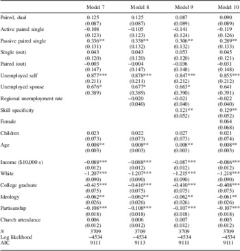
Table 3 reports ordered logit regression results summarizing our findings from the GSS data. After conditioning on observable confounding factors, we find results that mirror those from the lab: relative to every other dependency group, those with a partner in the labor force but who were not themselves working were significantly more likely to favor increased spending on unemployment benefits. To allay concerns about the multicollinearity between gender and dependency status, Models 7 through 9 omit gender while Model 10 includes it. None of the other estimated coefficients in the model are affected by the presence of gender in the model. Compared with the estimated effect of being the dependent partner in a two person household, other conditions are essentially indistinguishable from one another. We also find that those currently unemployed or with an unemployed partner are much more supportive of unemployment benefits, consistent with Margalit (Reference Margalit2013). Note that the point estimate for own unemployment is estimated with considerably more precision and is about 20 percent larger than that for partner’s unemployment. Neither the number of children in the household nor the regional unemployment rate is a significant predictor of support for unemployment benefits. Interestingly, gender fails to show any predictive power once we account for dependency status.
Ordered Logistic Regression Parameter Estimates for Support for Social Insurance in General Social Survey (GSS)

Note: Survey wave dummies and threshold parameters for the ordered logit regression were estimated for all models but are not reported in the table.
AIC=Akaike information criterion.
***p<0.01, **p<0.05, *p<0.1.
Findings for the other covariates are in line with the existing literature: whites, higher income individuals, those with more education, and more conservative respondents all are less supportive of unemployment spending. Contrary to Scheve and Stasavage (Reference Scheve and Stasavage2008), religiosity is not an important predictor here. Skill specificity is a consistently positive and significant predictor of support for unemployment spending.
We check whether our dependency status results are in fact specific to unemployment by fitting similarly specified regressions for other questions that formed part of the government spending battery.Footnote 29 Results do not show the same pattern as we observed for unemployment benefits.Footnote 30 Dependents were no more likely to prefer increased spending on any of the programs included in the GSS questionnaire than people who were otherwise similar in terms of the demographics and political attitudes. Effects of asymmetric dependency appear concentrated on respondent evaluation of labor market risk rather than producing a general dispositional shift in attitudes toward government actions.
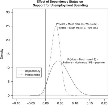
We provide a more expansive substantive interpretation for the model in Figure 4.Footnote 31 The solid line shows the distribution of the predicted effect of moving from “single only” (an unpartnered individual in the labor force) to “passive single” (the dependent member of a single-earner household). After controlling for observable demographic and attitudinal factors, our hypothetical dependent is about 5 percentage points more likely to support either “more” or “much more” spending on unemployment benefits.
Difference in the predicted probability of supporting “more” or “much more” spending on unemployment benefits Note: The solid line shows the distribution of the differences in probabilities between two otherwise similar individuals who differ in their dependency statuses. To demonstrate the substantive size of the effect, the dashed line shows the distribution of the predicted differences between two otherwise similar individuals who hold different political views (a “pure” independent and a weakly identifying Democrat, a two-point shift on the partisanship scale). All other variables in the model were held constant.

For comparison, the plot also shows the implied “effect” of moving two points in the Democratic direction on the partisan identification scale, from “Pure independent” to a weakly identifying Democrat (dashed line). The average predicted effect of asymmetric dependency is roughly equivalent to moving two points on the seven-point party identification scale, although the implied effect of the latter is more precisely estimated.
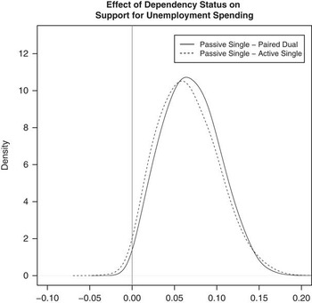
Holding income constant while going from a single earner to the stay-at-home member of a two adult household may not represent a realistic comparison. In Figure 5, we present a more realistic counterfactual. Given that total income covaries with the number of earners in a household, this figure shows the estimated difference in predicted probability of supporting more spending on unemployment benefits comparing an individual who is in a paired dual household with the average income of the other Paired Dual households in the sample (a little more than 0.5 SD above the mean level of income) to a dependent in a single-earner home with the average income of the other single-earner households in the sample (almost exactly the sample mean income). The estimated distribution of this effect is shown in the solid line of the figure.
Difference in the predicted probability of supporting “more” or “much more” spending on unemployment benefits Note: The solid line shows the distribution of the differences in probabilities between two otherwise similar individuals who differ on their dependency status and average income. The plot shows the difference between an individual in a paired single household with the average earnings of a single-earner household as the passive participant and an individual in a paired dual household with the average income of two-earner households. The dashed line shows the distribution of the difference between a dependent in a single-earner household and a similarly situated individual in a single-earner household who is in the labor force. All other variables in the model were held constant.

For comparison, the plot also includes the estimated difference in support for more unemployment benefits comparing an individual in the dependent role in a single-earner household with the individual in the labor force. For the purposes of this comparison, household income is held constant at the average level for single-earner households. The estimated difference in probability of support for unemployment benefits is almost indistinguishable from that of the dual-earner comparison.
In sum, we find evidence that our lab findings relating asymmetric dependency status to preferences for social insurance are also visible in observational survey data. The effect of asymmetric dependency is both consistent and substantively large.
Conclusion
Much of the literature on the political economy of the welfare state assumes atomistic individuals, ignoring the ties of mutual and often asymmetric economic dependency that bind us together in households. While evidence from psychology, marketing, and behavioral economics suggests that dependency relationships should matter for how individuals and households approach risky choices and form preferences for insurance, such insights have not been explored in a political context. This paper represents a first step toward integrating these literatures, focusing on a core policy domain: partial insurance against job loss.
We report the results of a laboratory experiment designed to directly investigate whether dependency on another for income in risky circumstances affects people’s support for social insurance policies. Unlike previous research, our experiment explicitly removes any redistributive considerations. We viewed our treatment as quite weak, posing a strong test for the existence of any dependency effect. Our most novel finding is that asymmetric dependency—being dependent on someone else for income when they are not dependent on you—increased subjects’ willingness to support income insurance policies, at least when the risk of job loss is not too high. Mutual dependency did not appear to induce any behavior different from what we observe from single individuals. In an effort to demonstrate that these findings are in fact relevant outside our highly stylized lab setting, we took our main results to observational survey data from the United States. While such findings are not causally identified, we do find additional evidence that closely mirrored what we observed in the more controlled (and contrived) lab environment: asymmetric dependency, that is, those dependent on others for their well-being are more supportive of unemployment insurance once we condition on a variety of other known covariates.
Two important caveats are in order. First, our weak (non-)finding of any mutual dependency effect in the lab may be due to the fact that we failed to induce a strong enough bond between partners. Future work might explore different ways of increasing the solidarity in pairs by, for example, using a sample of real-life couples, allowing communication, showing an image of the partner, or simply giving the pairs a name or identity around which to coordinate. Second, we did not explore whether within-subjects changes in dependency status changed subjects’ views toward social insurance, again an obvious extension for future work.
Our findings leave the question of mechanisms unresolved. What are the psychological, social, or other processes that give rise to this asymmetry in dependency effects? We can only speculate at this point. For example, we could be observing an “agency effect” where those lacking some semblance of control over the generation of their money income are more supportive of insurance. Or asymmetric dependency could induce feelings of vulnerability. If either reaction exists, how permanent or transitory is it? Other mechanisms are surely possible and future work is needed.
Another open question relating to mechanisms is the extent to which our findings travel to different national and cultural contexts. All our data and subjects were drawn from the United States. It may be that people with exposure to different gender norms, unemployment insurance policies, or “varieties of capitalism” may react differently. For example, countries where publicly provided services (such as health care) are widespread and not means tested may see a less pronounced asymmetry effect.
Historically, the vast majority of asymmetrically dependent individuals have been women in homemaker and caretaker roles. In our lab study all interactions were anonymous, instructions were gender-neutral, and partnerships could not be dissolved. We abstracted away from gender roles in dependency relationships, yet we still found that dependency matters. Moreover, in our experiment, we found no significant gender gap in support for social insurance. In the survey data, we found that gender is not a significant predictor of support for social insurance once we accounted for dependency status. It appears that individuals’ policy preferences respond to local, relationship-specific dependency in addition to broader gendered differences in labor force opportunities and public policy.
Finally, our findings have an important implication for observational studies: if the asymmetric dependency result is stable and consistent then we should observe important spatial and diachronic variation in the support for social insurance as women entered the labor force in greater numbers and marital stability fluctuated.
Supplementary Material
To view supplementary material for this article, please visit http://dx.doi.org/10.1017/psrm.2015.58