


INTRODUCTION
Theoretical models of lawmaking in the spirit of pivotal politics integrate policy makers’ preferences and institutions to understand legislative outcomes (Krehbiel Reference Krehbiel1998; Brady and Volden Reference Brady and Volden2006; Cox and McCubbins Reference Cox and McCubbins2005; Chiou and Rothenberg Reference Chiou and Rothenberg2009). These models typically assume that policy makers vote sincerely, at least for final passage votes. Sincere voting implies that institutions affect only agenda setting and how votes are aggregated. This independence of institutions and voting behavior allows theorists to analyze the role of institutions taking policy makers’ voting behavior as fixed. Likewise, it allows empiricists to recover policy makers’ preferences from roll call votes independently of the institutional settings (e.g., Poole and Rosenthal Reference Poole and Rosenthal1985; Heckman and Snyder Reference Heckman and Snyder1997; Clinton, Jackman, and Rivers Reference Clinton, Jackman and Rivers2004).Footnote 1
These models of lawmaking, however, are inherently static and take the current status quo as exogenous. In reality, policy makers periodically revise policies to respond to changing circumstances. Thus, the current status quo is inherited from previous votes, and is therefore endogenous. As highlighted by the game theoretic literature (e.g., Baron Reference Baron1996; Kalandrakis Reference Kalandrakis2004; Riboni and Ruge-Murcia Reference Riboni and Ruge-Murcia2008; Penn Reference Penn2009; Duggan and Kalandrakis Reference Duggan and Kalandrakis2012; Bernhardt and Buisseret Reference Bernhardt and Buisseret2017), the endogeneity of the status quo can distort policy makers’ incentives in important ways.Footnote 2 The goal of this paper is to introduce dynamics into models of pivotal politics to reexamine the mapping between legislative environment and legislative outcomes. In particular, we investigate how voting behavior varies with political institutions and expectations about future economic and political shocks.
We analyze an infinite-horizon extension of an otherwise parsimonious model of lawmaking. A set of policy makers repeatedly chooses between two policies, and the policy implemented in a given period can be revised in the next period only if a decisive coalition under the prevailing institution agrees to do so. Policy makers’ preferences over these two policies are redrawn in each period in a stochastic fashion, but their relative ideological positions remain constant. The shocks to the preferences capture changes in the relative efficiency or popularity of the policies, for instance due to economic crises, changes in demographic trends, international events, or simply the vagaries of public opinion.
The equilibrium analysis reveals that under all institutions with some degree of checks and balances, policy makers do not vote sincerely. Specifically, all equilibria exhibit two main patterns. First, consistent with the findings in Dziuda and Loeper (Reference Dziuda and Loeper2016), the voting behavior exhibits strategic polarization: relative to sincere voting, any two policy makers disagree more frequently. As a result, the government gridlocks more frequently. Second, policy makers may exhibit an average policy bias: the voting behavior of the government as a whole can be tilted toward a particular policy on average. This bias affects the relative prevalence of liberal versus conservative policy reforms, relative to sincere voting. Importantly, the degree of strategic polarization and direction of policy bias depend on the details of the political institution.
The intuition for these distortions is as follows. For institutions with checks and balances, one can identify two distinct policy makers whose agreement is needed for a policy change (Krehbiel Reference Krehbiel1998; Brady and Volden Reference Brady and Volden2006). Following Krehbiel (Reference Krehbiel1998), we call these policy makers pivots. Since the status quo stays in place whenever the pivots disagree, policy makers have incentives to affect which policy is the future status quo by distorting their votes today. Rightist and leftist policy makers disagree on which policy should be the status quo. As a result, relative to their sincere preferences, the former vote more frequently for the conservative policy and the latter more frequently for the liberal policy, leading to an increase in gridlock. Moreover, this strategic polarization effect may not affect the two sides of the political spectrum symmetrically. Depending on who the pivots are, and thus depending on the states in which they disagree, the policy makers on average may prefer one policy to be the status quo. As a result, the government as a whole may exhibit a bias in the direction of this policy.
One might argue that our theory is observationally indistinguishable from the static theory of voting, the only difference being that static models treat policy makers’ voting behavior as the sincere expression of their intrinsic preferences, whereas our model interprets it as a more complex equilibrium object. However, this apparent equivalence overlooks an important point. In the dynamic model, voting behavior is no longer independent of the institutions. This implies that when predicting the impact of institutional changes, one cannot take as given the policy preferences revealed by current or past votes.
This brings us to the central result of the paper, namely, how static and the dynamic models differ in their analysis of institutional change. Consider an increase in the size of coalitions required to implement a liberal policy change, for example, an increase in the institutional hurdle to raise taxes. A static model makes two predictions. First, a more rightist policy maker becomes pivotal for a liberal policy change. This means that the pivots are more ideologically polarized, which increases gridlock. Second, since the policy maker pivotal for a conservative policy change remains the same, liberal reforms become less frequent relative to conservative ones. Our analysis shows that these two predictions need to be qualified. First, the strategic polarization effect implies that a static model underestimates the inertial effect of this institutional change. In our dynamic setting, the considered institutional change increases the likelihood of future gridlock, and thus increases policy makers’ incentives to defend their preferred status quo for tomorrow, relative to voting for the policy that they sincerely prefer today. As a result, they vote in a more polarized way, increasing gridlock further. Second, the average policy bias effect implies that a static model overestimates the policy bias of this institutional change. In our dynamic setting, increasing the institutional hurdle to pass liberal reforms makes liberal policy makers less willing to adopt conservative reforms when needed, by fear of not being able to revert to more liberal policies once the environment changes. This decreases the incidence of conservative policies compared to the static model. In other words, the average policy bias works against any exogenous policy bias embedded in the voting institution. We further show that this strategic effect can be so strong that the institutional bias in favor of conservative policies can actually increase the incidence of liberal policies in the long run.
The last finding is not of purely theoretical interest. In the last decades, several U.S. states have passed constitutional amendments that require a qualified majority to increase taxes. These amendments were designed to reduce spending and tax levels. In a similar spirit, the U.S. Congress voted every year between 1996 and 1999 on an amendment to require two-thirds supermajority to enact tax increases. Our results imply that such amendments can exacerbate the polarization of these legislatures, and thus severely limit their ability to react to political and economic shocks. More surprisingly, these amendments can even fail to achieve their primary goal of keeping taxes low.
Our model reveals another important determinant of policy makers’ behavior, which by assumption is absent from static models, namely policy makers’ expectations. We first investigate the impact of expectations about the future policy environment. Specifically, we show that policy makers vote in a more polarized manner on issues on which their preferences are expected to be more volatile. That is, there is more gridlock precisely in domains in which the policy should respond quickly to frequent shocks. This finding implies that when designing institutions, checks and balances should be weaker for such policy domains. A prominent example is taxation: tax policies must react to varying factors such as the business cycle or investors’ expectations about fiscal sustainability. Our findings suggest that procedural rules that limit the power of the filibuster, such as the reconciliation process, can be particularly beneficial in such volatile policy areas.
Second, we investigate the impact of policy makers’ expectations about the future political environment. To do so, we extend the model and allow for political turnover. We show that policy makers’ voting behavior depends on their expectation about the composition of the next government because the latter determines the likelihood of future gridlock, and thus the incentives for policy makers to distort their vote and defend their preferred status quo. For example, if policy makers expect the next government to be united, the future status quo is unlikely to matter, so they vote more in line with their sincere preferences. Conversely, if they expect the next government to be divided, they bias their voting behavior significantly. An important insight of our model is that the equilibrium voting behavior depends on the composition of the future, but not on the current government. In particular, a perfectly united government may vote strategically. For example, a united conservative government may decrease taxes even in times of high budget deficit to secure a more favorable status quo in case the next government is divided.
One of the puzzles of recent years has been an increase in polarization of policy makers in the U.S. Congress as inferred from their voting behavior (see, e.g., McCarty, Poole, and Rosenthal Reference McCarty, Poole and Rosenthal2008). The goal of this paper is to analyze lawmaking in the simplest dynamic setting; hence, we abstract from many aspects of lawmaking that may speak to this increase in polarization.Footnote 3 Nevertheless, our results suggest three possible factors that may have contributed to it. First, concurrently with the rise in measured polarization, the filibuster—once an infrequently used tool reserved for the most salient and controversial bills—has become a routine practice in American politics (see Koger Reference Koger2010; chap. 5 of Binder and Smith Reference Binder and Smith1997; or Wawro and Schickler Reference Wawro and Schickler2006). Some political scientists and pundits blame the more frequent use of the filibuster on the increase in policy makers’ ideological polarization (Krehbiel Reference Krehbiel1998; McCarty Reference McCarty, Pierson and Skocpol2007). Our results suggest a possible reverse causality: the change in institutional practice de facto introduced more checks and balances, and hence made more extreme policy makers pivotal. This, according to our analysis, increases the incentives of all legislators to defend their preferred status quo, and thus should result in a greater degree of strategic polarization. Second, since the 1970s, divided governments have become increasingly common in the U.S. (e.g., Fiorina Reference Fiorina1994). Arguably, this should affect policy makers’ expectations about future gridlock. According to our results, such a change in expectations should push policy makers to vote in a more polarized way, even during the times of united government. And finally, even if ideological polarization is indeed on the rise, our results suggest that empirical studies might have overestimated the magnitude of such increase. In the dynamic model, any increase in ideological polarization is magnified by an increase in strategic polarization.
Our model is sparse, but as a result, it is tractable and can be easily extended to analyze substantive questions related to legislative bargaining, as illustrated in the Role of Expectations section. Moreover, unlike many dynamic models of legislative bargaining, it is not plagued by issues of multiplicity of equilibria types and equilibria indeterminacy, and hence makes clear predictions.
The paper is organized as follows. The next section discusses related literature. The Model section describes the basic model. The Equilibrium section characterizes the equilibrium in the benchmark static game (Static Model section) and in the dynamic game (Dynamic Model section). The Institutions and Voting Distortions section investigates the impact of institutions on equilibrium behavior and provides a welfare analysis. The Role of Expectations section analyzes how policy makers’ behavior varies with their expectations about the future policy and political environment. The Conclusion section concludes. All proofs are in the Appendix.
RELATED LITERATURE
Our paper is a dynamic extension of the static models of lawmaking in the spirit of pivotal politics, such as Krehbiel (Reference Krehbiel1998), Brady and Volden (Reference Brady and Volden2006), Cox and McCubbins (Reference Cox and McCubbins2005), or Chiou and Rothenberg (Reference Chiou and Rothenberg2009). We simplify the legislative bargaining game to isolate the impact of forward-looking considerations on voting behavior.
The paper closest to ours is Dziuda and Loeper (Reference Dziuda and Loeper2016), who analyze a similar model with two players and the unanimity rule. They show that equilibrium behavior exhibits strategic polarization. We show that strategic polarization extends to N players with arbitrary voting rules (Proposition 2) and further show that equilibrium behavior also exhibits an average bias effect (Corollary 3). More importantly, we analyze the impact of institutions on the strategic polarization effect (Proposition 4) and the average bias effect (Proposition 5). Our setup allows us to compare the voting behavior of different policy makers for a given voting rule, and the voting behavior of a given policy maker across different voting rules (Proposition 4), which is not possible in the two-player setup. As explained in the Institutions and Strategic Polarization section, disentangling the effect of ideology and institutions on voting behavior is key to understanding why a static approach underestimates the inertial effect of checks and balances.Footnote 4 Finally, we consider simple parametric specifications for the distribution of economic and political shocks that allow us to analyze how equilibrium behavior depends on players’ expectations (Propositions 7, 8, and 9).
Strategic voting has been studied in the context of amendments (Austen-Smith Reference Austen-Smith1987; Anesi and Seidmann Reference Anesi and Seidmann2014) and log-rolling (Clinton and Meirowitz Reference Clinton and Meirowitz2004). Since we consider only two policies and focus on stationary equilibria, the rationale for these voting strategies is absent in our model. Callander and Krehbiel (Reference Callander and Krehbiel2014) consider a dynamic environment with changing preferences, but assume that the default policy remains in the gridlock interval, so no policy change by legislature can be implemented. They focus instead on benefits of power delegation to an agency: risk-averse legislators are willing to delegate policy-making power to an agency to commit to state-dependent policy. Commitment by means of delegation would also be desirable in our setting.
The implications of the dynamic linkage between today’s policy and tomorrow’s status quo have been studied by a growing literature on dynamic legislative bargaining. This literature finds that the endogenous status quo can generate equilibrium distortions of various kinds (see, e.g., Baron Reference Baron1996; Kalandrakis Reference Kalandrakis2004; Roberts Reference Roberts2007; Penn Reference Penn2009; Bowen, Chen, and Eraslan Reference Bowen, Chen and Eraslan2014; Baron and Bowen Reference Baron and Bowen2015; Diermeier, Egorov, and Sonin Reference Diermeier, Egorov and Sonin2017) and lead to inefficient outcomes (Anesi and Seidmann Reference Anesi and Seidmann2015; Anesi and Duggan forthcoming; Buisseret and Bernhardt Reference Bernhardt and Buisseret2017).Footnote 5 These papers assume fixed preferences, and the only impetus for policy change is the changing identity of the proposer, the ability of the proposer to build new coalitions over time and/or the random arrival of new alternatives. We focus instead on situations in which the impetus for policy change comes from shocks to the policy makers’ preferences. In this respect, Riboni and Ruge-Murcia (Reference Riboni and Ruge-Murcia2008), Zapal (Reference Zapal2011) and Duggan and Kalandrakis (Reference Duggan and Kalandrakis2012) are closer to our paper. They, however, do not identify the polarizing effect of an endogenous status quo and do not study how voting behavior varies with the voting rule and players’ expectations. At a technical level, our policy space is meant to capture a one-dimensional ideological conflict, and does not allow costs and benefits to be freely allocated among policy makers. As a result, the analysis is not plagued by the equilibrium indeterminacy and complexity problems highlighted by Anesi and Seidmann (Reference Anesi and Seidmann2015) and Anesi and Duggan (2017), and, in particular, our predictions do not depend on how players vote when indifferent (Anesi and Seidmann Reference Anesi and Seidmann2015; Baron and Bowen Reference Baron and Bowen2015).
The literature on voting rules argues that under simple majority, undesirable policies can be passed (Buchanan and Tullock Reference Buchanan and Tullock1962) whereas supermajority requirements can block or delay good policies (Tsebellis Reference Tsebellis2002; Compte and Jehiel Reference Compte and Jehiel2010). Our paper shows that static models underestimate the severity of the latter effect. Several papers analyze the impact of voting rules in dynamic settings (Eraslan and Merlo Reference Eraslan and Merlo2002; Harstad Reference Harstad2005; Battaglini and Coate Reference Battaglini and Coate2007, Reference Battaglini and Coate2008; Strulovici Reference Strulovici2010; Acemoglu, Egorov, and Sonin, Reference Acemoglu, Egorov and Sonin2015). These papers differ from ours in that, in those papers, the current policy affects players’ future payoff, information, or political power. Piguillem and Riboni (Reference Piguillem and Riboni2013, Reference Piguillem and Riboni2015) argue that the status quo inertia induced by the endogenous status quo can provide a beneficial commitment device to legislators with time-inconsistent preferences. Diermeier, Egorov, and Sonin (Reference Diermeier, Egorov and Sonin2017) show in a purely distributive setting that the set of stable allocations does not necessarily increase with the degree of consensus required by the voting rule.
MODEL
Players and Policies
A set of policy makers  $\mathcal {N}=\left\lbrace 1,\ldots ,n,\ldots ,N\right\rbrace$ are in a relationship that lasts for infinitely many periods. Time is discrete and, in each period, they must decide which of the two policies L and R to implement, where L can be interpreted as a liberal policy such as a high tax rate, high public-spending level, or high level of protection of domestic industries, and R as its conservative counterpart.
Payoffs
Each policy maker  $n\in \mathcal {N}$ maximizes her expected discounted sum of period payoffs with discount factor δ ∈ (0, 1). Her payoff from implementing policy R in some period
 $t\in \mathbb {N}$ is denoted by θn(t), and her payoff from implementing L is normalized to 0. Hence, if θn(t) is positive (negative), policy maker n prefers the conservative policy R (the liberal policy L) in t. One can view this specification as a stylized dynamic extension of the canonical spatial model in which θn(t) is the peak of policy maker n’s single-peaked utility function.Footnote 6 We refer to θn(t) as the sincere preferences of policy maker n in period t. Throughout, we use bold symbols to denote N-tuples, and use the symbol
 $\boldsymbol{\theta }$ and the term “state” to refer to a particular realization of the random variable
 $\boldsymbol{\theta }\left(t\right) \equiv \left( \theta _{1}\left( t\right) ,\ldots ,\theta _{N}\left( t\right) \right)$.
We assume that the stochastic process  $\left\lbrace \boldsymbol{\theta }\left( t\right) :t\in \mathbb {N} \right\rbrace$ that governs the evolution of the state is i.i.d. across periods, with probability distribution P. We assume that P is such that for all
 $n\in \mathcal {N}$, θn(t) is integrable, has full support,Footnote 7 and satisfies the following properties:
Assumption 1 For all  $t\in \mathbb {N} ,$
(A) θ1(t) < . . . < θN(t) with probability one;
(B) for any
 $n,m\in \mathcal {N}$ with n < m, θn(t) < 0 < θm(t) with positive probability.

Assumption 1(A) states that even though policy makers’ preferences evolve over time, their ideological rank order remains constant. Specifically, those with lower indices are more leftist than those with higher indices. Therefore, whenever two policy makers disagree, the relatively more leftist always prefers L and the relatively more rightist prefers R. This assumption is in line with Poole and Rosenthal (Reference Poole and Rosenthal1991), who find that “Congress as a whole may adapt by, for example, moving to protectionism when jobs are lost to foreign competition. But as such new items move onto the agenda, their cutting lines will typically be consistent with the preexisting, stable voting alignments.”Footnote 8 Assumption 1(B) means that any two legislators disagree with positive probability.
The Legislative Game
In each t, a status quo q(t) ∈ {L, R} is in place. First,  $\boldsymbol{\theta }\left( t\right)$ is realized and each policy maker
 $n\in \mathcal {N}$ observes her own preferences θn(t).Footnote 9 Then she chooses whether to vote for the status quo or the alternative policy. If the set of policy makers who vote for the alternative policy is a winning coalition, this policy is implemented. Otherwise, the status quo stays in place. The implemented policy determines the payoffs for period t and becomes the status quo for the next period q(t + 1).
The Institutions
In our stylized environment, the institutional arrangement is summarized by the set of winning coalitions needed for a policy change. We allow this set to depend on the identity of current status quo: for all q ∈ {L, R}, Ωq denotes the set of winning coalitions when the status quo is q, Ω denotes (ΩL, ΩR), and Γ(Ω) denotes the game thus defined. We impose the following conditions on Ω:
Assumption 2 For all q ∈ {L, R},
(A) Monotonicity: if C ∈ Ωq and C⊂C′, then C′ ∈ Ωq,
(B) Nonemptyness:
$\mathcal {N}\in \Omega _{q},$(C) Properness: if C ∈ Ωq and q′ ≠ q, then N∖C∉Ωq′.

Assumption 2 is standard in the literature on voting (see, e.g., Austen-Smith and Banks Reference Austen-Smith and Banks1999). Monotonicity ensures that an additional vote in favor of an alternative can only change the outcome in favor of that alternative. Nonemptyness means that a unanimous vote for a given alternative guarantees that this alternative is implemented irrespective of the status quo. Properness requires that if a coalition can change the policy in place, those outside this coalition cannot reverse this change.
Assumption 2 allows for a large class of institutions. For instance,
 $$\begin{equation}
\Omega _{R}=\Omega _{L}=\Omega ^{M}\equiv \left\lbrace C\subseteq \mathcal {N} :\left|C\right|\ge M\right\rbrace
\end{equation}$$
corresponds to a parliamentary system with a single chamber operating under a supermajority rule with threshold M. Assumption 2 is satisfied for all M ≥ (N + 1)/2. The two polar cases M = (N + 1)/2 and M = N correspond to the simple majority rule and the unanimity rule, respectively. Assumption 2 allows also for nonanonymous institutions, such as the combination of simple majority rule and a veto player (or gate keeper)  $v\in \mathcal {N}$:
 $$\begin{equation}
\Omega _{R}=\Omega _{L}=\Omega ^{v}\equiv \left\lbrace C\subseteq \mathcal {N} :C\in \Omega ^{\left( N+1\right) /2}\text{ and }v\in C\right\rbrace.
\end{equation}$$
Nonanonymous institutions are the de facto rules in many democracies in which the legislative body uses simple majority but is subject to the negative agenda control of the majority leader, or the veto power of the president.Footnote 10
Equilibrium
As standard for dynamic voting games, we look for stationary Markov perfect equilibria in stage-undominated strategies (henceforth, equilibria) as defined in Baron and Kalai (Reference Baron and Kalai1993). A stationary Markov strategy for player n in Γ(Ω) maps the realization of  $\boldsymbol{ \theta }\left( t\right)$ and the status quo into a probability distribution over {L, R}. Stage undomination requires that in each period, each player votes for the policy that gives her the greater continuation payoff. This equilibrium refinement rules out pathological equilibria such as all players always voting for the status quo. We assume that when indifferent, a player votes for R, but this assumption is made only for expositional convenience and does not affect the results.
Comments on Assumptions
We abstract from many aspects of lawmaking to isolate the sole impact of introducing dynamics. In particular, our policy makers are purely policy motivated and we abstract from elections. We introduce elections in a reduced form in the Role of Expectations section.
The policy space consists of two alternatives, which is clearly an abstraction, albeit a useful one. Since there is only one alternative to the status quo, this assumption implies that in each period, the bill under consideration is exogenous and cannot be amended. As a result, we do not need to specify details of how bills and amendments are chosen, and can completely characterize the political decision process by collections of winning coalitions Ω. This allows us to focus on differences between static and dynamic models without keeping track of differences among static models.Footnote 11 Note also that our results do not rely on the absence of “compromise” alternatives that lie between L and R. In a setting with two players and the unanimity rule, Dziuda and Loeper (Reference Dziuda and Loeper2016) show that under reasonable assumptions on the bargaining procedure, similar voting distortions arise when players can chose from a one-dimensional space of alternatives, and there is no reason to suspect that the same would not hold in the setting of this paper.Footnote 12 Allowing for more alternatives, however, would come at a significant cost in terms of technical and expositional complexity.
We consider policies that are continuing in nature: policies that do not have an expiration date and remain in effect until a new agreement is reached. Many policies have this feature. In the U.S., this is the case of most tax policies (Gale and Orszag Reference Gale and Orszag2003) and most spending policies: by law, all mandatory spending is continuing and this spending category, which contains all entitlements, represents more than two-thirds of the total federal budget (Levit, Austin, and Stupak Reference Levit, Austin and Stupak2015). Similarly, labor laws and minimum wage legislation tend to be continuing in nature (Clinton Reference Clinton2012). Sunset provisions, that is, clauses that attach an expiration date to a legislation, historically have been the exception rather than the norm.
EQUILIBRIUM
Static Model
Since most of the lawmaking literature in the spirit of pivotal politics is static, we first consider as a benchmark the game Γ0(Ω) in which policy makers play only the first period t = 0 of Γ(Ω). In the unique equilibrium of this game, each policy maker n votes sincerely. That is, she votes for R if θn(0) ≥ 0 and for L if θn(0) < 0, irrespective of the status quo. As argued in the pivotal politics literature (see, e.g., Krehbiel Reference Krehbiel1998), sincere voting implies the existence of two decisive players, called pivots, such that a policy change occurs if and only if these two pivots vote for it.
To see who these pivots are, consider first status quo L, and suppose that θn(0) ≥ 0, so legislator n votes for R. Assumption 1(A) implies that with probability 1, all more rightist policy makers k ≥ n also vote for R. So if {n, . . ., N} ∈ ΩL, then R is implemented. Suppose now that θn(0) < 0, so n votes for L instead. Assumption 1(A) implies that only strictly more rightist policy makers k > n may vote for R. Hence, if {n + 1, . . ., N}∉ΩL, then L stays in place. So if n is such that
 $$\begin{equation}
\left\lbrace n,\ldots ,N\right\rbrace \in \Omega _{L}\text{ and }\left\lbrace n+1,\ldots ,N\right\rbrace \notin \Omega _{L},
\end{equation}$$
then under status quo L, the equilibrium outcome always coincides with n’s vote. Conditions A and B in Assumption 2 guarantee that Equation (3) characterizes a unique n, which we label l(Ω) and refer to as the left pivot.Footnote 13 The right pivot, which we denote by r(Ω), is defined in a symmetric fashion by n such that
 $$\begin{equation}
\left\lbrace 1,\ldots ,n\right\rbrace \in \Omega _{R}\text{ and }\left\lbrace 1,\ldots ,n-1\right\rbrace \notin \Omega _{R}.
\end{equation}$$
The following proposition summarizes the above analysis:
Proposition 1 The unique equilibrium of Γ0(Ω) is sincere voting: each policy maker  $n\in \mathcal {N}$ votes for R if and only if θn(0) ≥ 0. If the status quo is L (R), policy maker l(Ω) (r(Ω)) is pivotal in the sense that with probability 1, the equilibrium outcome coincides with her vote.
Since the mapping between institutions and pivots plays a crucial role in our analysis, in the example below, we show how pivots are determined for the examples of institutions introduced in the Model section.
Example 1 Consider five players and, for expositional simplicity, assume the following common-shock specification: for all n and  $t\in \mathbb {N} ,$
 $\theta _{n}\left( t\right) =\bar{\theta }_{n}+\varepsilon \left( t\right) ,$ where
 $\boldsymbol{\bar{\theta }}\in \mathbb {R} ^{N}$ and the stochastic process
 $\left\lbrace \varepsilon \left( t\right) :t\in \mathbb {N} \right\rbrace$ is i.i.d. with mean 0. If ε(t) has full support and
 $\bar{\theta }_{n}$ is strictly increasing in n, this specification satisfies Assumption 1. The ideological ordering of policy makers corresponds to the ordering of their average preferences
 $\boldsymbol{\bar{\theta }},$ like in Figure 1. The common shock ε(t) captures the shock to the policy environment in period t. Consider first simple majority, denoted by ΩM = 3 as defined in Equation (1). The coalition of policy makers {3, 4, 5} is winning but {4, 5} is not, so Equation (3) implies that l(ΩM = 3) = 3. Likewise, {1, 2, 3} is winning, but {1, 2} is not, so from Equation (4), r(ΩM = 3) = 3. That is, policy maker 3 is both the left and the right pivot.
Determination of the pivots for the 4/5th majority rule.

Consider now supermajority ΩM = 4, that is, the rule which requires four votes for a policy change. The determination of pivots under this institution is illustrated in Figure 1. Under ΩM = 4, {2, 3, 4, 5} is a winning coalition but {3, 4, 5} is not, so Equation (3) implies that l(ΩM = 4) = 2. Also, {1, 2, 3, 4} is winning, but {1, 2, 3} is not, so from Equation (4), r(ΩM = 4) = 4.
And finally, consider the institution Ωv = 2 defined in Equation (2) in which policy changes must be approved both by a simple majority and by the veto player, policy maker 2. The coalition {2, 3, 4, 5} is winning as it contains both a majority of policy makers and the veto player, but {3, 4, 5} is not, as it does not include the veto player, so from Equation (3), l(Ωv = 2) = 2. Likewise, {1, 2, 3} is winning, but {1, 2} is not, because it does not form a majority. Hence, Equation (4) implies that r(Ωv = 2) = 3.
In Example 1, l(Ω) ≤ r(Ω). More generally, conditions (A) and (C) in Assumption 2 imply that this inequality always holds.Footnote 14 That is, the left pivot is always weakly more leftist than the right pivot. When l(ΩL) = r(ΩR), we shall say that Ω is quasi-dictatorial: the equilibrium outcome of Γ0(Ω) is the same as if the unique pivot were the dictator. Quasi-dictatorial institutions include dictatorship, but also non-dictatorial institutions such as simple majority rule. When l(ΩL) < r(ΩR), we shall say that Ω is non-quasi-dictatorial. Examples of non-quasi-dictatorial institutions include supermajority requirements, bicameral governments, or unicameral governments with a presidential veto.
In the pivotal politics literature, the influence of the status quo for a given institution is captured by the gridlock interval, defined as the set of status quos that cannot be replaced by any proposal (Krehbiel Reference Krehbiel1998). In our model, any status quo may be replaced if the realization of  $\boldsymbol{\theta }\left( t\right)$ makes it sufficiently unappealing. However, for any profile of votes, either the same policy is implemented irrespective of the status quo, or the current status quo stay in place.Footnote 15 Hence, it seems natural to adapt the canonical notion of gridlock as follows.
Definition 1 For any institution Ω, strategy profile  $\boldsymbol{\sigma },$ and
 $\boldsymbol{\theta }\in \mathbb {R} ^{N}$, we say that gridlock occurs in state
 $\boldsymbol{\theta }$ if the actions prescribed by
 $\boldsymbol{\sigma }$ when
 $\boldsymbol{\theta } \left( t\right) =\boldsymbol{\theta }$ are such that the current status quo q(t) stays in place independent of whether q(t) = L or q(t) = R.
From Proposition 1, in the equilibrium of Γ0(Ω), gridlock occurs in state  $\boldsymbol{ \theta }$ if the pivots’ sincere preferences disagree in that state. Since l(Ω) ≤ r(Ω), in that case, l(Ω) prefers L and r(Ω) prefers R. So the set of gridlock states is
 $$\begin{equation}
G^{0}\left( \Omega \right) =\lbrace \boldsymbol{\theta }\in \mathbb {R} ^{N}:\theta _{l\left( \Omega \right) }<0\le \theta _{r\left( \Omega \right) }\rbrace.
\end{equation}$$
For instance, for the environment considered in Example 1 and ΩM = 4, the set of gridlock states in equilibrium is  $G^{0}\left( \Omega ^{M=4}\right) =\lbrace \varepsilon \in \mathbb {R} ^{N}:\bar{\theta }_{2}<-\varepsilon \le \bar{\theta }_{4}\rbrace$. In Figure 1, this is the area between
 $\bar{\theta }_{2}$ and
 $\bar{\theta }_{4}.$
Dynamic Model
In the dynamic game Γ(Ω), policy makers’ votes determine not only today’s policy, as in the static game Γ0(Ω), but also tomorrow’s status quo, which in turn affects future payoffs. Let W n(q) denote the value of the game Γ(Ω) for policy maker n given initial status quo q ∈ {L, R}. In any period t, her continuation payoff from implementing R is θn(t) + δW n(R) and from implementing L is 0 + δW n(L). So the stage-undominated action for n is to vote for R if and only if
 $$\begin{equation}
\theta _{n}\left( t\right) +\delta \left( W_{n}\left( R\right) -W_{n}\left( L\right) \right) \ge 0.
\end{equation}$$
Denote d n ≡ δ(W n(R) − W n(L)). By comparison with Γ0(Ω), we see that in equilibrium, n behaves as if the game was static but her preferences were θn(t) + d n instead of θn(t). We call the term θn(t) + d n her strategic preferences in t, and d n her voting distortion.Footnote 16 The voting distortions  $\boldsymbol{d}$ reflect policy makers’ preferences over the next status quo.
Let us first investigate when sincere voting, that is,  $\boldsymbol{d}=\left( 0,\ldots ,0\right) ,$ can be an equilibrium. Consider the environment of Example 1, and suppose first that Ω is the simple majority rule. If policy makers vote sincerely in Γ(Ω), then as argued in Example 1, voter 3 is pivotal under either status quo, so her most preferred policy is always implemented. Therefore, in any period t, the status quo does not affect the future policy path, and hence W n(R) = W n(L). So by Equation (6), it is optimal for policy makers to vote sincerely. Note that the same argument holds for any quasi-dictatorial rule.
Consider now the case of a non-quasi-dictatorial institution, say the 4/5th majority rule as in Example 1 and Figure 1. If policy makers vote sincerely, then policy makers 2 and 4 are the pivots. From Assumption 1(B), the sincere preferences of these pivots disagree with positive probability; hence, there are states in which the status quo stays in place. In those states, policy maker 2 prefers policy L and policy maker 4 prefers policy R, and hence W 2(L) > W 2(R) and W 4(L) < W 4(R). Therefore, by Equation (6), sincere voting cannot be an equilibrium.
How do policy makers distort their vote when Ω is non-quasi-dictatorial? For any profile of votes, either the outcome of the vote is the same irrespective of the status quo, or both status quos stay in place. So status quo R is weakly more likely to result in policy R than status quo L. Therefore, policy makers with more rightist policy preferences also have more rightist preferences over the next status quo. Given Assumption 1(A), this means that d n = W n(R) − W n(L) increases in n. The latter property implies that in any equilibrium, policy makers’ strategic preferences  $\boldsymbol{\theta }\left( t\right) +\boldsymbol{d}$ are rank-ordered as their sincere preferences
 $\boldsymbol{\theta }\left( t\right).$ That is, more rightist policy makers should vote in a more rightist way. As a result, in equilibrium, the same players as in Γ0(Ω) are pivotal under each status quo, and by the same argument as before, l(Ω) and r(Ω) distort their vote in favor of L and R, respectively.
The following proposition formalizes the above intuition:
Proposition 2 An equilibrium of Γ(Ω) exists. For any equilibrium, there exists a unique  $\boldsymbol{d} \in \mathbb {R} ^{N}$ such that in any period
 $t\in \mathbb {N} ,$ each policy maker
 $n\in \mathcal {N}$ votes for R if and only if θn(t) + dn ≥ 0. As in the static game Γ0(Ω), in any period in which the status quo is L (R), policy maker l(Ω) (r(Ω)) is pivotal in the sense that the equilibrium outcome coincides with her vote with probability 1.
If Ω is quasi-dictatorial, then the unique equilibrium is sincere voting, that is,
$\boldsymbol{d}=\left( 0,\ldots ,0\right)$.If Ω is non-quasi-dictatorial, then in any equilibrium,
(i) d1 < .. < dN,
(ii) dl(Ω) < 0 < dr(Ω).

Proposition 2 has three noteworthy implications. First, policy makers vote sincerely in Γ(Ω) only when Ω is quasi-dictatorial. Second, when Ω is non-quasi-dictatorial, in any equilibrium, the voting distortions  $\boldsymbol{d}$ have a polarizing effect. To see this, note that from Assumption 1(A) and Proposition 2(i), for any non-quasi-dictatorial Ω, with probability 1,
 $$\begin{eqnarray}
&&\left|\left( \theta _{n}\left( t\right) +d_{n}\right) -\left( \theta _{m}\left( t\right) +d_{m}\right) \right| = \left|\left( \theta _{n}\left(t\right)\right.\right.\nonumber\\
&&\quad\left.\left. -\theta _{m}\left( t\right) \right) +\left( d_{n}-d_{m}\right) \right| >\left|\theta _{n}\left( t\right) -\theta _{m}\left( t\right) \right|.
\end{eqnarray}$$
The distance between the strategic preferences of policy makers n and m on the left-hand side of Equation (7) can be interpreted as their degree of strategic polarization. Hence, Equation (7) states that under any non-quasi-dictatorial rule, the degree of strategic polarization between any two policy makers is greater than their degree of ideological polarization |θn(t) − θm(t)|.
Finally, Proposition 2 has important implications for policy dynamics. In any equilibrium of Γ(Ω), pivots have the same decisive role as in Γ0(Ω), so gridlock occurs in state  $\boldsymbol{\theta }$ if the pivots’ strategic preferences disagree in that state. In such states, l(Ω) votes for L and r(Ω) votes for R. Therefore, in any equilibrium with distortions
 $\boldsymbol{d}$, the set of gridlock states is
 $$\begin{equation}
G\left( \Omega \right) =\lbrace \boldsymbol{\theta }\in \mathbb {R} ^{N}:\theta _{l\left( \Omega \right) }+d_{l\left( \Omega \right) }<0\le \theta _{r\left( \Omega \right) }+d_{r\left( \Omega \right) }\rbrace.
\end{equation}$$
When comparing Equation (5) to Equation (8), Proposition 2(ii) implies that the set of gridlock states is greater—in the inclusion sense—in any equilibrium of Γ(Ω) than in the equilibrium of Γ0(Ω). Thus, the strategic polarization that arises in the dynamic game exacerbates gridlock: policy change occurs less frequently than predicted by the static model.Footnote 17
The next proposition characterizes the equilibrium distortions. Recall that d n is defined as δ(W n(R) − W n(L)), that is, policy maker n′s preference over the next status quo, and the latter matters only if the next state is in the gridlock interval. In any gridlock state, either status quo stays in place, so the continuation payoff gain of having status quo R instead of L is given by θn(t) + δ(W n(R) − W n(L)). This delivers the following:
Proposition 3 For all  $\boldsymbol{d}\in \mathbb {R} ^{N}$, there exists an equilibrium of Γ(Ω) whose profile of voting distortions is
 $\boldsymbol{d}$ if and only if for all
 $n\in \mathcal {N},$
 $$\begin{equation}
d_{n}=\delta \int _{\boldsymbol{\theta }\in G\left( \Omega \right) }\left( \theta _{n}+d_{n}\right) dP\left( \boldsymbol{\theta }\right) ,
\end{equation}$$
where G(Ω) is given by Equation (8). In particular, in any equilibrium,
 $$\begin{eqnarray}
\frac{1}{N}\sum \nolimits _{n\in \mathcal {N}}d_{n} &=&\frac{\delta }{1-\delta P\left( G\left( \Omega \right) \right) }\nonumber\\
&&\times\int _{\boldsymbol{\theta }\in G\left( \Omega \right) }\left( \frac{1}{N}\sum \nolimits _{n\in \mathcal {N} }\theta _{n}\right) dP\left( \boldsymbol{\theta }\right). \qquad
\end{eqnarray}$$
Note that, in general, the right-hand side of Equation (10) does not need to be 0, which means that policy makers’ average strategic preferences  $\frac{1}{N}\sum _{n\in \mathcal {N}}\left( \theta _{n}\left( t\right) +d_{n}\right)$ may be more rightist or leftist than their average sincere preferences
 $\frac{1}{N}\sum _{n\in \mathcal {N}}\theta _{n}\left( t\right)$. Hence, policy makers may exhibit an average policy bias: they may vote as if they were on average biased toward one alternative. Note that this bias depends on the preference distribution across policy makers, but also on the political institution via G(Ω). Whereas strategic polarization increases the probability of gridlock, the average bias affects the relative likelihood of liberal versus conservative policy change, and thus the relative prevalence of policies L and R. We explore the effect of the policy bias more carefully in the Biased Institutions section.
Remark 1 Proposition 3 implies that the equilibria are easy to characterize. One must first solve Equation (9) for n = l(Ω) and n = r(Ω); that is, solve a (nonlinear) system of two equations with two unknowns. Any solution (dl(Ω), dr(Ω)) pins down the gridlock set G(Ω). Once G(Ω) is determined, for n∉{l(Ω), r(Ω)}, Equation (9) becomes a straightforward linear equation in dn. Moreover, in symmetric setups, dr(Ω) = −dl(Ω), so the behavior of the pivots is characterized by a single equation.Footnote 18 For instance, for the specification in Example 1, if F is the distribution of ε(t), this equation becomes
 $$\begin{eqnarray}
&&\hspace*{-7pt}d_{r\left( \Omega \right) }\nonumber\\
&&\quad\hspace*{-7pt} =\frac{\delta \left( F\left( d_{r\left( \Omega \right) }+\bar{\theta }_{r\left( \Omega \right) }\right) -F\left( -d_{r\left( \Omega \right) }-\bar{\theta }_{r\left( \Omega \right) }\right) \right) }{ 1-\delta \left( F\left( d_{r\left( \Omega \right) }+\bar{\theta }_{r\left( \Omega \right) }\right) -F\left( -d_{r\left( \Omega \right) }-\bar{\theta } _{r\left( \Omega \right) }\right) \right) }\bar{\theta }_{r\left( \Omega \right) }. \nonumber\\
\end{eqnarray}$$
Propositions 2 and 3 imply a fundamental difference between static and dynamic models. At first sight, the predictions of these models seem observationally equivalent. In both, each policy maker votes for the policy closer to her ideal point, the only difference being that in the static theory, this ideal point reflects her sincere preference θn(t), whereas in the dynamic theory the ideal point θn(t) + d n is also affected by strategic, forward looking considerations. However, this apparent equivalence overlooks an important point. First and foremost, the static approach treats policy makers’ preferences as an independent primitive. In contrast, Proposition 2 implies that preferences are equilibrium objects, and as such, are endogenous to the political decision process Ω. Hence, when considering the impact of institutional changes, one cannot take as given the preferences as revealed by the current legislative behavior, but has to understand how these strategic preferences change with Ω. Second, policy makers’ strategic preferences depend crucially on their expectations about the future gridlock. Hence, changes in expectations, even when not accompanied by observable changes in the current institution or environment, are likely to affect current behavior.
Having established that institutions and expectations about future economic and political environment shape policy makers’ behavior, it is important to better understand the mapping between the former and the latter. We do this in the Institutions and Voting Distortions and Role of Expectations sections.
Before we proceed, however, we note that the game Γ(Ω) may have multiple equilibria.Footnote 19 This is because gridlock feeds on itself: if policy makers expect more frequent future gridlock, they have greater incentives to distort their vote for the policy they prefer in case of gridlock, and this in turn increases the likelihood of gridlock. One can prove, however (see Lemma 1 in the Appendix) that equilibria can be ranked in terms of the degree of strategic polarization of the pivots. Formally, we say that an equilibrium with distortions  $\boldsymbol{d}^{\prime }$ is strictly more polarized than another equilibrium with distortions
 $\boldsymbol{d}$ if d′l(Ω) < d l(Ω) and d′r(Ω) > d r(Ω). Then for any two distinct equilibria, one is strictly more polarized than the other. In what follows, when multiplicity is an issue, the comparative statics are derived for the least polarized equilibrium (which always exists), but the same results hold for the most polarized equilibrium.
INSTITUTIONS AND VOTING DISTORTIONS
Institutions and Strategic Polarization
In this section, we investigate how the equilibrium voting behavior depends on voting institutions. We use the following partial order on institutions.
Definition 2 Let Ω and Ω′ be two institutions. We say that Ω′ requires a greater consensus than Ω if Ω′L⊆ΩL and Ω′R⊆ΩR.
In other words, Ω′ requires a greater consensus than Ω if changing the status quo requires the approval of a greater set of policy makers under Ω′ than under Ω. For example, rules that use a higher supermajority threshold require a greater consensus, and adding a veto player, or more generally adding checks and balances, increases the degree of consensus required. By definition of l(Ω) and r(Ω), an institution that requires a greater consensus leads to more extreme pivots.Footnote 20 Formally, if Ω′ requires a greater consensus than Ω, then
 $$\begin{equation}
l(\Omega ^{\prime })\le l\left( \Omega \right) \le r\left( \Omega \right) \le r(\Omega ^{\prime }).
\end{equation}$$
Proposition 4 Let Ω and Ω′ be two institutions and let  $\boldsymbol{d}\left( \Omega \right)$ and
 $\boldsymbol{d}\left( \Omega ^{\prime }\right)$ denote the voting distortions of the least polarized equilibrium of Γ(Ω) and Γ(Ω′), respectively. If Ω′ requires a greater consensus than Ω, then
 $$\begin{eqnarray}
d_{l\left( \Omega ^{\prime }\right) }\left( \Omega ^{\prime }\right) &\le& d_{l\left( \Omega ^{\prime }\right) }\left( \Omega \right) \le d_{l\left( \Omega \right) }\left( \Omega \right) \le 0\le d_{r\left( \Omega \right) }\left( \Omega \right)\nonumber\\
& \le& d_{r\left( \Omega ^{\prime }\right) }\left( \Omega \right) \le d_{r\left( \Omega ^{\prime }\right) }\left( \Omega ^{\prime }\right) ,
\end{eqnarray}$$
and for all  $n,m\in \mathcal {N}$, with probability 1,
 $$\begin{eqnarray}
&&\left|\left( \theta _{n}\left( t\right) +d_{n}\left( \Omega ^{\prime }\right) \right) -\left( \theta _{m}\left( t\right) +d_{m}\left( \Omega ^{\prime }\right) \right) \right|\nonumber\\
&&\quad\ge \left|\left( \theta _{n}\left( t\right) +d_{n}\left( \Omega \right) \right) -\left( \theta _{m}\left( t\right) +d_{m}\left( \Omega \right) \right) \right|. \qquad
\end{eqnarray}$$
If, furthermore, (l(Ω), r(Ω)) ≠ (l(Ω′), r(Ω′)), then the outer inequalities in Equation (13) and the inequality in Equation (14) are strict.
The first claim in Proposition 4 states that increasing the required consensus exacerbates the voting distortions of the left and right pivot in favor of policy L and R, respectively, and does so for two reasons. First, from Equation (12), more extreme policy makers become pivots, and from Proposition 2, for a fixed institution Ω, more extreme policy makers have greater voting distortions. This effect explains the four inner inequalities in Equation (13). Second, the voting distortions of the new pivots are greater under Ω′ than under Ω, which results in the two outer inequalities in Equation (13). The latter effect comes from the fact that as more extreme players become pivots, the probability that pivots disagree, and thus that gridlock occurs in the future increases. The greater likelihood of future gridlock in turn increases the incentives of each new pivot to distort her vote in favor of her preferred status quo.
Inequalities in Equation (13) imply that the pivots exhibit a greater degree of strategic polarization under the rule that requires a greater consensus. The inequalities in Equation (14) state that the same is true for any two policy makers.
An important consequence of Proposition 4—illustrated in Figure 2 for the common-shock specification of Example 1—is that the static and the dynamic approaches predict different impact of institutional change. To see why, note that when assessing the impact of a change from Ω to Ω′, the static approach assumes that policy makers’ past voting behavior under Ω, as given by their strategic preferences  $\left( \theta _{n}\left( t\right) +d_{n}\left( \Omega \right) \right) _{n\in \mathcal {N}}\!,$ is sincere, and thus that they would continue voting the same way under Ω′. Given the new pivots l(Ω′) and r(Ω′), the static approach would then conclude that gridlock under Ω′ would occur when
 $$\begin{equation*}
\theta _{l\left( \Omega ^{\prime }\right) }\left( t\right) +d_{l\left( \Omega ^{\prime }\right) }\left( \Omega \right) < 0\le \theta _{r\left( \Omega ^{\prime }\right) }\left( t\right) +d_{r\left( \Omega ^{\prime }\right) }\left( \Omega \right).
\end{equation*}$$
The dynamic approach implies instead that gridlock under Ω′ occurs when
 $$\begin{equation*}
\theta _{l\left( \Omega ^{\prime }\right) }\left( t\right) +d_{l\left( \Omega ^{\prime }\right) }\left( \Omega ^{\prime }\right) <0\le \theta _{r\left( \Omega ^{\prime }\right) }\left( t\right) +d_{r\left( \Omega ^{\prime }\right) }\left( \Omega ^{\prime }\right).
\end{equation*}$$
The two outer inequalities in Equation (13) imply hence that the static approach underestimates the inertial effect of replacing Ω by Ω′, by not taking into account policy makers’ behavior change.
The top picture illustrates static gridlock under ΩM = 4 for the common-shock specification. The middle picture illustrates policy makers’ strategic preferences and the gridlock under ΩM = 4 as well as the gridlock predicted by static models when the institution changes to ΩM = 5 taking the behavior of policy makers under ΩM = 4 as sincere. The bottom picture illustrates the actual gridlock under ΩM = 5.

These results provide potentially testable implications. Consider an institutional reform that increases the degree of consensus required for policy changes, such as adding a second chamber, allowing presidential veto, or replacing simple with a qualified majority. Then any two policy makers who are in office before and after the reform takes place should exhibit a greater degree of polarization in their voting behavior after the reform is implemented.
Proposition 4 also speaks to the impact of filibuster in the U.S. Senate. Pundits often argue that the U.S. Senate should abandon the filibuster since the increased ideological polarization makes it hard to gather 60 votes on virtually any important legislation. Proposition 4 implies that indeed abandoning the institution of the filibuster should decrease gridlock in the U.S. Congress, not only because the approval of fewer senators would be required to pass a policy change, but also because the voting behavior of all U.S. congressmen should become less polarized. This logic also suggests an alternative interpretation of the correlation between the more frequent use of the filibuster and the growing polarization among the U.S. legislators. The filibuster was once an infrequently used tool reserved for the most important and controversial bills, but since the ’70s it has become a routine practice in American politics (Koger Reference Koger2010). At the same time, polarization in Congress started increasing (McCarty, Poole, and Rosenthal Reference McCarty, Poole and Rosenthal2008). Pundits tend to interpret the rise in the use of the filibuster as a tactic used by a more ideologically polarized Senate to stifle reforms. Our results suggest a possible alternative explanation. The new norm of systematically using the filibuster de facto shifted the pivotality in the U.S. Congress—not only in the U.S. Senate—to more ideologically polarized policy makers. Hence, Proposition 4 predicts that this de facto institutional change should have resulted in more polarized voting behavior and an increase in gridlock.
Biased Institutions
Some democratic institutions use different voting rules depending on the policy change under consideration. For example, in sixteen U.S. states, tax increases require the approval of a qualified majority in each house, whereas tax cuts can be approved by simple majority. Similarly, in the U.S. budget process, the Byrd Rule essentially requires a filibuster-proof majority to pass bills that raise deficit, whereas simple majority is sufficient to pass bills that lower it.Footnote 21 The explicit goal of these fiscally conservative institutions was to limit growth of the public sector and the public debt. Indeed, within a static framework, increasing a hurdle for a policy change in one direction decreases the probability that such policy change occurs. However, the analysis below shows that once the strategic effects are taken into account, fiscally conservative voting rules can induce a more liberal voting behavior on average, and can even lead to more liberal policies. This insight is consistent with the empirical finding that effects of such biased voting rules on the level of state taxes in the U.S. have been modest, if any.Footnote 22 It is also consistent with the observation that the Byrd rule did not prevent the federal debt from growing steadily since its implementation.
Definition 3 An institution Ω is biased in favor of policy R if l(Ω) + r(Ω) > N.
To see why the inequality in Definition 3 corresponds to an institution biased for policy R, observe that from Proposition 2, status quo L is replaced by R when all policy makers in {l(Ω), . . ., N} vote for R. Conversely, status quo R is overturned when all policy makers in {1, . . ., r(Ω)} vote for L. So the condition l(Ω) + r(Ω) > N means that a greater coalition is needed to repeal R than to repeal L. For instance, if Ω requires a supermajority with threshold M q under status quo q, then Ω is biased in favor of R if and only if M L < M R.
Proposition 5 below identifies a class of environments in which the government as a whole has no ideological bias, but when operating under a rule biased in favor of R, the average voting bias makes it vote as if it was in favor of L on average.
Proposition 5 Consider the common shock specification like in Example 1, that is, for all  $n\in \mathcal {N}$ and
 $t\in \mathbb {N} ,$
 $\theta _{n}\left( t\right) =\bar{\theta }_{n}+\varepsilon \left( t\right)$. If
 $\boldsymbol{\bar{\theta }}$ and ε(t) are symmetrically distributed around 0, and if Ω is biased in favor of R, then in any equilibrium, the average voting distortion is biased in favor of L, that is,
 $\frac{1}{N}\sum _{n}d_{n}<0$.
Under the conditions of Proposition 5, when Ω is unbiased, L and R receive the same expected number of votes. Proposition 5 states that when Ω is biased in favor of R, the expected number of votes for L is greater. The intuition for that result is that policy makers anticipate that it may be hard to replace R with L in the future, and are therefore more inclined to vote for L today. Thus, in our dynamic setting, increasing the institutional hurdle to pass liberal reforms makes not only liberal reforms, but also conservative reforms less likely to be implemented.
Proposition 5 raises a question whether the increase in the expected number of votes for L may be large enough to offset the institutional bias in favor of R. Example below shows that the answer is affirmative: biasing political institution against, say, liberal policy reforms, always reduces the likelihood of both liberal and conservative reforms, but may also result in policies that are more liberal on average.
Example 2 Consider the common-shock specification like in Example 1, where ε(t) follows a standard normal distribution. Unlike in Proposition 5, however, assume that the government is ideologically biased toward L, with median policy maker’s ideological position  $\bar{\theta }_{\left( N+1\right) /2}=-0.5$. Under the simple majority rule ΩM = (N + 1)/2, the median voter is always pivotal, and there are no voting distortions; hence, the probability that L is implemented in any period is
 $\Pr \left( -0.5+\varepsilon <0\right) =\Phi \left( 0.5\right) =0.7.$ Suppose now that the hurdle to implement L increases. The median policy maker remains the left pivot, whereas a more rightist policy maker becomes the right pivot,
 $\bar{\theta }_{r}>-0.5.$ Hence, the probability that R is replaced by L goes down, and is equal to
 $\Phi \left( -\bar{\theta } _{r}-d_{r}\right) <\Phi \left( -\bar{\theta }_{r}\right) <\Phi \left( 0.5\right) $. However, the median policy maker distorts her voting behavior in favor of L, d(N + 1)/2 < 0, so the probability that L is replaced by R also goes down,
 $1-\Phi \left( -\bar{\theta }_{\left( N+1\right) /2}-d_{\left( N+1\right) /2}\right) <1-\Phi \left( 0.5\right) $. Hence, in terms of taxes, making a voting rule biased against tax increases makes both tax increases and decreases less likely.
Figure 3 depicts the probability of L according to the stationary distribution of the underlying Markov process over policies; that is, the probability that in a distant future the policy is L for the biased voting rule (solid line) and for simple majority (dashed line). Increasing the bias in favor of R, which is equivalent to increasing  $\bar{\theta }_{r},$ does not monotonically increase the long-run prevalence of R, and it can even make L more likely to be implemented in the long run.Footnote 23
Probability that L is in place in the long run a function of the bias of the voting rule in favor of R.

Voting Distortions and Welfare
The proposition below states that the greater the voting distortions of the pivots, and thus the greater gridlock, the worse off the moderate policy makers are.
Proposition 6 Let  $\boldsymbol{d}$ and
 $\boldsymbol{d}^{\prime }$ be the voting distortions of two equilibria of Γ(Ω), with
 $\boldsymbol{d}^{\prime }$ being strictly more polarized than
 $\boldsymbol{d}$. Then all policy makers n ∈ {l(Ω), . . ., r(Ω)} are strictly better off in the equilibrium with distortions
 $\boldsymbol{d}$. Moreover, if Ω′ requires a greater consensus than Ω and (l(Ω), r(Ω)) ≠ (l(Ω′), r(Ω′)), then all n ∈ {l(Ω), . . ., r(Ω)} are strictly better off in the least polarized equilibrium of Γ(Ω) than in the least polarized equilibrium of Γ(Ω′).
To see the intuition for this result, consider an equilibrium and suppose that the right pivot deviates by voting for R in a greater set of states (because an institutional change makes the pivot ideologically more extreme, and/or because she increases her voting distortion). This deviation is detrimental to all legislators more leftist than her because the outcome under status quo R is less likely to coincide with their preferences. The best response of the left pivot to this deviation is to become more biased in favor of L, so as to avoid status quo R, and this is detrimental to all legislator more rightist than her for the same reason.
It is worth pointing out, however, that our model abstracts from many aspects of policy making that could make checks and balances and the resulting inertia desirable. For example, our policy makers do not have dynamic inconsistency problem (Piguillem and Riboni Reference Piguillem and Riboni2013, Reference Piguillem and Riboni2015) that gridlock could solve, two policies leave no room for policy smoothing across periods (Bowen, Chen, and Eraslan Reference Bowen, Chen and Eraslan2014; Bowen et al. Reference Bowen, Chen, Eraslan and Zapal2017), and majorities have limited flexibility to design policies concentrating benefits and spreading the costs (Baron Reference Baron1991; Battaglini and Coate Reference Battaglini and Coate2007, Reference Battaglini and Coate2008), which precludes the tyranny Role of Expectations even under rules that require little consensus.
ROLE OF EXPECTATIONS
The intuition for the equilibrium distortions provided in the Equilibrium section highlights the role of policy makers’ expectations about the policy environment (how preferences over policies evolve) and political environment (who the pivots may be). In this section, we investigate how policy makers’ voting behavior depends on these expectations. We first analyze the impact of the expected volatility of policy makers’ preferences. Second, we allow for political turnover and consider the impact of policy makers’ expectation about the composition of future governments.
Volatility of the Environment
The realization of  $\boldsymbol{\theta }\left( t\right)$ can be interpreted as the current economic situation, state of knowledge, or citizens’ sentiment. In some areas, these variables are likely to change more frequently than in others. We investigate now how strategic polarization and gridlock depend on policy maker’s expectations about the volatility of the policy environment.
To this end, we relax the assumption that the state is i.i.d. over time. Instead, we assume that in each t ≥ 1, conditional on  $\boldsymbol{ \theta }\left( t-1\right) ,$
 $\boldsymbol{\theta }\left( t\right) = \boldsymbol{\theta }\left( t-1\right)$ with probability 1 − v, and with probability v,
 $\boldsymbol{\theta }\left( t\right)$ is redrawn independently of previous states, and according to the same probability distribution P as in the basic model. Thus, v ∈ [0, 1] measures the volatility of the environment.Footnote 24
Policy gridlock is bound to be particularly detrimental in environments in which frequent policy changes are a desirable response to a volatile environment. In the next proposition, we show that, unfortunately, it is in such environments that strategic polarization, and hence gridlock, tend to be greater.
Proposition 7 Let Ω be a non-quasi-dictatorial institution, and let  $\boldsymbol{d}$ and
 $\boldsymbol{d}^{\prime }$ be the voting distortions of the least polarized equilibrium of Γ(Ω) with volatility v and v′, respectively, with 0 < v < v′ ≤ 1. Then
 $$\begin{equation*}
d_{l\left( \Omega \right) }^{\prime }<d_{l\left( \Omega \right) }<0<d_{r\left( \Omega \right) }<d_{r\left( \Omega \right) }^{\prime }.
\end{equation*}$$
When the environment is static—that is, v = 0—then in the unique equilibrium,  $\boldsymbol{d}=\left( 0,..,0\right) $.
The intuition for Proposition 7 is as follows. As the volatility of the environment increases, the policy implemented today is more likely to require revision tomorrow; hence, securing a favorable status quo becomes more important relative to implementing the sincerely preferred policy today.
Proposition 7 suggests that the impact of the environment volatility on the likelihood of policy change is ambiguous. As volatility increases, more frequent shocks prompt more frequent policy changes, but policy makers become strategically more polarized, and are thus less likely to agree on policy response after shocks. Figure 4 above demonstrates that the latter effect may dominate, and policy persistence may be greater in environments that require more frequent policy reforms.
Probability that policy changes from one period to another as a function of preference volatility.

Figure 4 considers again the common shock specification from Example 1 with Ω generating symmetric pivots, that is,  $\bar{\theta }_{r\left( \Omega \right) }=-\bar{\theta }_{l\left( \Omega \right) }=0.5$. For this environment, Figure 4 depicts policy volatility—measured by the probability that the policy changes in the next period—as a function of v. Initially, these two volatilities move together. This is because for low volatility, the strategic effect is small. However, as volatility becomes large, the strategic effect dominates and the policy becomes more persistent.
Tax, welfare, or trade are prominent examples of volatile policy domains. The goal of most tax reforms oscillate between stimulating the economy (i.e., lowering tax rates) and reducing the deficit (i.e., increasing tax rates). These reforms are prompted by recurring shocks such as business cycles, changes in fiscal needs, or the vagaries of public opinion. Likewise, since WWII, welfare policies have had to adapt to the emergence of new social risks, growing inequalities, and changing demographics (Hacker Reference Hacker2004). Trade policies must also react to sectorial shocks, domestic pressures, and the international environment. Proposition 7 provides a rationale for procedural rules that limit the degree of consensus required in such areas. Examples of such rules include the reconciliation process, which limits the use of the filibuster for fiscal policies, or the fast track authority, which limits the ability of Congress to veto the decisions of the president for trade policies (Koger Reference Koger2010; Howell and Moe Reference Howell and Moe2016).
Political Turnover
The basic model assumes that policy makers stay in office indefinitely. Realistically, elections imply political turnover. To investigate how turnover shapes behavior, we extend the model as follows. Let  $\mathcal {N}=\left\lbrace 1,\ldots ,N\right\rbrace$ denote the set of political positions (e.g., presidency, congressional seats), and
 $\mathcal {C} =\left\lbrace 1,\ldots ,C\right\rbrace$ the set of potential candidates for these positions. In any period
 $t\in \mathbb {N}$, the preferences of each candidate
 $c\in \mathcal {C}$ are denoted by
 $\theta _{c}\left( t\right) \in \mathbb {R}$ and the candidate elected in each position
 $n\in \mathcal {N}$ is denoted by
 $e_{n}\left( t\right) \in \mathcal {C}$. The institution Ω specifies coalitions of political positions that are winning, independently of which candidates are currently appointed to these positions, and Ω is assumed to satisfy Assumption 2.
In each period t, before voting, candidates commonly observe the preferences  $\boldsymbol{\theta }\left( t\right)$ and the electoral outcome
 $\boldsymbol{e}\left( t\right) $. To capture policy makers’ expectation about the future political environment, we assume that they also observe a common signal
 $s\left( t\right) \in \mathcal {S}$ that conveys information about the next elections
 $\boldsymbol{e}\left( t+1\right) $. For example, s(t) may contain information that more leftist candidates are more likely to be elected next period. To retain the stationarity of the model, we assume that
 $\left\lbrace \left( \boldsymbol{\theta }\left( t\right) ,s\left( t\right) ,\boldsymbol{e}\left( t\right) \right) :t\in \mathbb {N} \right\rbrace$ is a stationary process. To make sure that s(t) only captures electoral expectations, we further assume that for all t ≥ 1,
 $\boldsymbol{\theta }\left( t\right)$ and s(t) are independent of the past and of
 $\boldsymbol{e}\left( t\right) ,$ whereas
 $\boldsymbol{e}\left( t\right)$ is correlated with the past only via s(t − 1). In line with Assumption 1, the rank order of the candidates’ preferences is fixed, but we slightly relax that assumption to allow some candidates to have the same preferences. Formally, for all t, θ1(t) ≤ . . . ≤ θC(t) with probability 1. To keep this extension in line with the basic model, we assume that each candidate c cares about the implemented policy independent of whether she is in office.Footnote 25
Proposition 8 In any equilibrium, there exists a profile of functions  $\boldsymbol{d}\left( .\right)$ from
 $\mathcal {S}$ to
 $\mathbb {R}$ such that for all
 $t\in \mathbb {N} ,$ a candidate
 $c\in \mathcal {C}$ elected in period
 $t\in \mathbb {N}$ votes for R if and only if θc(t) + dc(s(t)) ≥ 0. For all realizations
 $s\in \mathcal {S}$ of the signal, d1(s) ≤ . . . ≤ dC(s).
Proposition 8 is a natural extension of Proposition 2, but reveals an interesting point overlooked by the latter. Voting distortions do not depend on which candidates are currently in office,  $\boldsymbol{e}\left( t\right) $. Instead, they depend on policy makers’ expectations about who will be in office tomorrow, as captured by s(t). To see why, recall that policy makers distort their votes to influence which alternative prevails in case of future gridlock, and the latter depends only on who is elected tomorrow, not today. Note, however, that the electoral outcome
 $\boldsymbol{e}\left( t\right)$ still affects the policy outcome in t, as it determines who is pivotal in that period.
To illustrate the applicability of this extension, consider a simple case in which candidates can be of two types, say Republicans and Democrats, and suppose that these types disagree with positive probability in the sense of Assumption 1(B). The electoral outcome  $\boldsymbol{e}\left( t\right)$ can lead to one of three cases: either there exists a winning coalition of elected Democrats, or there exists a winning coalition of elected Republicans, or no winning coalition of the same type exists. The first two cases correspond to a united government, whereas the last case corresponds to a divided government.
Proposition 9 For all  $s\in \mathcal {S},$ let
 $\Pr \left( Div|s\right)$ denote the probability that conditional on s(t) = s, the government is divided in period t + 1, that is, no winning coalition is of the same type. Then in any equilibrium, there exists dDem < 0 < dRep such that for all c ∈ {Dem, Rep} and all
 $s\in \mathcal {S},$
 $d_{c}\left( s\right) =d_{c}\Pr \left( Div|s\right)$.
Thus, Democrats distort their voting behavior in favor of L and Republicans in favor of R. Moreover, voting distortions depend not on whether the current government is divided, but on the probability that it is divided in the future, and are increasing in the latter. The intuition for that result is as follows. When the government is united, a winning coalition of Democrats or of Republicans can unilaterally implement any policy irrespective of the status quo. Conversely, when the government is divided, with positive probability, no policy receives a bipartisan support, in which case either status quo stays in place. Hence, if policy makers expect future government to be united, they do not care about the future status quo and vote sincerely, whereas if they expect future government to be divided, they are biased in favor of their most preferred status quo.
A careful analysis of the differences between united and divided governments in a dynamic setting is beyond the scope of this paper. It is interesting, however, that policy distortions occur even under united government. To see that, consider a united Republican government that inherited high tax rates from the previous government. Suppose further that because of a high level of public debt, both parties sincerely prefer to leave those rates unchanged. Republicans may nevertheless decrease them to assure a favorable status quo should they need Democrats’ approval to implement a tax cut in the future.
The last proposition generalizes Proposition 9 to an arbitrary number of types. For any realization of the electoral outcome  $\boldsymbol{e}\left( t\right)$, one can reorder the political positions from the position held by the most leftist appointee to the position held by the most rightist appointee, keeping unchanged the role of each position in Ω. One can then define the left and right pivots as in the Static Model section. Proposition 8 implies that, almost surely, θ1(t) + d 1(s(t)) ≤ . . . ≤ θC(t) + d C(s(t)). That is, more rightist appointees vote in a more rightist way, so for almost all realizations of
 $\boldsymbol{\theta }\left( t\right)$ and s(t), the outcome of the vote under status quo L (R) coincides with the vote of the left (right) pivot given
 $\boldsymbol{e}\left( t\right)$, as in the basic model.
Proposition 10 For all  $\left( l,r\right) \in \mathcal {C}^{2}$ and s ∈ S, let
 $\Pr \left( l,r|s\right)$ denote the probability that
 $\boldsymbol{e}\left( t+1\right)$ is such that the left and right pivots in t + 1 are candidates l and r, respectively, conditional on s(t) = s. Then in any equilibrium, for all
 $c\in \mathcal {C}$, there exists
 $\left( \Delta _{c}\left( l,r\right) \right) _{1\le l<r\le C}\in \mathbb {R} ^{\frac{C\left( C+1\right) }{2}}$ such that for s ∈ S,
 $$\begin{equation*}
d_{c}\left( s\right) =\sum _{1\le l<r\le C}\Pr \left( l,r|s\right) \times \Delta _{c}\left( l,r\right) .
\end{equation*}$$
Moreover, Δc(l, r) weakly decreases as l moves closer to c from either side, and weakly increases as r moves closer to c from either side.
Proposition 10 states that policy maker c’s distortion is more rightist the closer she expects to be to the next right pivot c r and the farther she expects to be from the next left pivot c l. The intuition for this is as follows. As in the basic model, the willingness to distort her vote in favor of R relative to L reflects her preferences over these policies conditional on pivots disagreeing. The more similar she expects to be to the right pivot and the more dissimilar she expects to be to the left pivot, the more likely she is to prefer R whenever the former votes for R and the latter votes for L.
Proposition 10 is derived in a stylized model; hence one has to exercise caution when applying it to the real world. Nevertheless, it is instructive to derive its implications in particular situations to illustrate its difference with the static approach.
Consider, for instance, presidential elections in which a Republican is expected to win with a coattail effect in the concurrent congressional elections. Since the coattail effect usually wanes in midterm elections, the expectations held before the presidential election about the ideology of the pivots right after the election are likely to be more rightist than the expectations held in the first two years of the presidency about the ideology of the pivots after the incoming midterm elections. Proposition 10 implies hence that moderate policy makers—including the legislator who becomes the left pivot during the first two years of the presidency—will vote in a more rightist way during the first two years of the presidency than during the two years before. So a government under Republican presidents may be more successful in replacing liberal status quos (i.e., L) by conservative policies (i.e., R) in her first two years not only because the ideology of the current president and Congress is more conservative, but also because their expectation of liberal shift in the next midterm elections increases their incentives to approve conservative policies today.
Finally, Proposition 10 suggests that the effects of the 1986 Supreme Court decisions on redistricting may be more nuanced than predicted by the static literature. Theoretically, redistricting increases expected ideological polarization of future delegations from the affected states. Suppose that redistricting happens in a conservative state with current representatives being to the right of the current right pivot. The expected right shift of some of its representatives will not affect who the future pivots are, but the shift of the remaining representatives to the left increases the probability that the future right pivot or even both pivots are more leftist candidates (see Shotts (Reference Shotts2003), for a discussion of how redistricting affects national legislature). Proposition 10 implies then that redistricting affects expectations in a way that makes moderate policy makers vote in a more rightist way.
CONCLUSIONS
Many modern democracies have a system of check and balances. Admittedly, these checks and balances are not designed to smooth the decision process. Rather, their role is to limit agency costs and the tyranny of the majority. Our model shows, however, that in policy domains in which the current agreement serves as the default for future negotiations, checks and balances tend to make policy makers more polarized, which can greatly exacerbate their inherently inertial effect. These distortions are most severe for policy areas in which timely responses to frequent exogenous shocks are desirable, and they are detrimental to welfare of the moderate policy makers (and presumably voters such policy makers’ represent). Hence, it is important to study institutional solutions that can mitigate these distortions without neutralizing the intended effects of checks and balances. One possibility is to use automatic indexation rules that tie the default to some verifiable variable that is correlated with the state of nature (see Weaver Reference Weaver1988; and Bowen et al. Reference Bowen, Chen, Eraslan and Zapal2017).
The tractability of our model provides an opportunity to study issues that are naturally considered in dynamic settings. For example, our model can be used to explore the incidence and impact of sunset provisions. Sunset provisions are clauses that determine an expiration date of a legislation (Gersen Reference Gersen2007). As such, they limit the endogeneity of the status quo, and hence the polarizing effect identified in this paper. In this light, understanding why sunset provisions are not used more frequently, and why their use changes over time is a natural next step for research.
APPENDIX
Notation 1 For any institution Ω, volatility v ∈ [0, 1], and profile of voting distortions  $\boldsymbol{d}\in \mathbb {R} ^{N},$ we denote
 $$\begin{equation}
G\left( \Omega ,\boldsymbol{d}\right) \equiv \left\lbrace \boldsymbol{\theta }\in \mathbb {R} ^{N}:\theta _{l\left( \Omega \right) }+d_{l\left( \Omega \right) }<0\le \theta _{r\left( \Omega \right) }+d_{r\left( \Omega \right) }\right\rbrace ,
\end{equation}$$
and for all  $n\in \mathcal {N}$ and all P-measurable
 $\Theta \subseteq \mathbb {R} ^{N}$,
 $$\begin{equation}
D_{n}\left( \Theta ,d_{n}\right) \equiv \frac{\delta v}{1-\delta +\delta v} \int _{\Theta }\left( \theta _{n}+d_{n}\right) dP\left( \boldsymbol{\theta } \right) .
\end{equation}$$
Proof of Proposition 1. Straightforward and hence omitted. ▪
Proof of Propositions 2 and 3. In the interest of space, these propositions are proven for the general model of the Volatility of the Environment section, in which, in any period t,  $\boldsymbol{\theta }\left( t\right)$ is redrawn with probability v ∈ [0, 1]. The basic model corresponds to the special case v = 1.
Equilibrium existence follows from Lemma 1(B), which is stated and proven next.Footnote 26 Step 1 below proves that any equilibrium is characterized by a unique profile of voting distortions  $\boldsymbol{d}$ (second claim of Proposition 2). Step 2 provides the necessary and sufficient condition for some
 $\boldsymbol{d}\in \mathbb {R} ^{N}$ to be the distortions of an equilibrium (first claim of Proposition 3). The expression for the average distortion in Proposition 3 is a direct corollary of that condition. Step 2 also proves that equilibrium distortions are ordered and result in the same pivots as in the static game (third claim of Proposition 2). Step 3 proves the rest of Proposition 2, namely that the distortions are
 $\boldsymbol{0}$ for any quasi-dictatorial institution and Propositions 2(i) and 2(ii) for any non-quasi-dictatorial institution.
Step 0: Notation.
Let  $\boldsymbol{\sigma }$ be a stationary Markov strategy profile,
 $n\in \mathcal {N}$,
 $\boldsymbol{\theta }\in \mathbb {R} ^{N},$ and x ∈ {L, R}. Denote by
 $W_{n}^{\boldsymbol{\sigma }}\left( x\right)$ the value for n of playing
 $\boldsymbol{\sigma }$ conditional on q(0) = x calculated before
 $\boldsymbol{\theta } \left( 0\right)$ is drawn according to P. Denote by
 $V_{n}^{\boldsymbol{ \sigma }}\left( \boldsymbol{\theta },x\right)$ the value for n of a strategy profile that implements x from period 0 until the first period t in which
 $\boldsymbol{\theta }\left( t\right) \ne \boldsymbol{\theta } \left( 0\right) $ and plays
 $\boldsymbol{\sigma }$ thereafter, conditional on
 $\boldsymbol{\theta }\left( 0\right) =\boldsymbol{\theta }$. Define
 $d_{n}^{\boldsymbol{\sigma }}\equiv \delta v\left[ W_{n}^{\boldsymbol{\sigma } }\left( R\right) -W_{n}^{\boldsymbol{\sigma }}\left( L\right) \right] $.
Step 1: For any equilibrium  $\boldsymbol{\sigma }$, there exists a unique
 $\boldsymbol{d}\in \mathbb {R} ^{N}$such that in any period
 $t\in \mathbb {N} ,$each policy maker n ∈ N votes for R if and only if θn(t) + d n ≥ 0. It is given by
 $\boldsymbol{d}=\boldsymbol{d}^{\boldsymbol{\sigma }}$, as defined in Step 0. Using the assumption that in each period t,
 $\boldsymbol{\theta }\left( t\right) =\boldsymbol{\theta }\left( t-1\right)$ with probability 1 − v and is redrawn from P with probability v, we have that for all
 $\boldsymbol{ \theta }\in \mathbb {R} ^{N},$
 $$\begin{eqnarray}
V_{n}^{\boldsymbol{\sigma }}\left( \boldsymbol{\theta },R\right) &=&\theta _{n}+\delta \left[ \left( 1-v\right) V_{n}^{\boldsymbol{ \sigma }}\left( \boldsymbol{\theta },R\right) +vW_{n}^{\boldsymbol{\sigma } }\left( R\right) \right]\nonumber\\
& =&\frac{\theta _{n}+\delta vW_{n}^{\boldsymbol{ \sigma }}\left( R\right) }{1-\delta \left( 1-v\right) }, \nonumber\\
V_{n}^{\boldsymbol{\sigma }}\left( \boldsymbol{\theta },L\right) &=&0+\delta \left[ \left( 1-v\right) V_{n}^{\boldsymbol{\sigma }}\left( \boldsymbol{ \theta },L\right) +vW_{n}^{\boldsymbol{\sigma }}\left( L\right) \right]\nonumber\\
& =& \frac{\delta vW_{n}^{\boldsymbol{\sigma }}\left( L\right) }{1-\delta \left( 1-v\right) }.
\end{eqnarray}$$
The Markov state in any period t consists of the realizations of  $\boldsymbol{\theta }\left( t\right)$ and q(t). The continuation payoff of implementing L or R in any such Markov state does not depend on q(t), so the stage-undominated actions remain the same as long as
 $\boldsymbol{\theta }\left( t\right)$ is not redrawn. Therefore, stage undomination (together with our tie-breaking rule) requires that n votes for R in state
 $\boldsymbol{\theta }$ if and only if
 $V_{n}^{\boldsymbol{\sigma }}\left( \boldsymbol{\theta },R\right) \ge V_{n}^{ \boldsymbol{\sigma }}\left( \boldsymbol{\theta },L\right)$. Using Equation (17), this inequality can be rewritten as
 $\theta _{n}+\delta v\left[ W_{n}^{\boldsymbol{\sigma }}\left( R\right) -W_{n}^{ \boldsymbol{\sigma }}\left( L\right) \right] \ge 0,$ and using the definition of
 $d_{n}^{\boldsymbol{\sigma }}$ from Step 0, it becomes
 $\theta _{n}+d_{n}^{\boldsymbol{\sigma }}\ge 0$. An equilibrium must satisfy this condition for all
 $\boldsymbol{\theta }$ in the support of P. Since θn(t) has full support,
 $d_{n}=d_{n}^{\boldsymbol{ \sigma }}$ is the only voting distortion that prescribes stage undominated actions in all states given continuation play
 $\boldsymbol{\sigma }$.
Step 2: For any  $\boldsymbol{d}\in \mathbb {R} ^{N}$,
 $\boldsymbol{d}$is the profile of voting distortions of an equilibrium of Γ(Ω) if and only if for all n ∈ N ,
 $d_{n}=D_{n}\left( G\left( \Omega ,\boldsymbol{d} \right),d_{n}\right) $. In any equilibrium, the corresponding voting distortions d n are (strictly) increasing in n (if
 $P\left( G\left( \Omega ,\boldsymbol{d}\right) \right) >0$), and policy makers l(Ω) and r(Ω) are pivotal under status quo L and R in the sense of Proposition 2.
First we show that if  $\boldsymbol{d}$ are the distortions of an equilibrium
 $\boldsymbol{\sigma }$, then
 $\boldsymbol{d}=\boldsymbol{D}\left( G\left( \Omega ,\boldsymbol{d}\right) ,\boldsymbol{d}\right)$, d n is increasing in n, and
 $\boldsymbol{\sigma }$ results in the same pivots as in the static game. From Step 1,
 $\boldsymbol{d}=\boldsymbol{d}^{ \boldsymbol{\sigma }}$. Since
 $\boldsymbol{d}^{\boldsymbol{\sigma }}$ does not depend on the status quo and Ω satisfies Assumption 2(C), on the path of
 $\boldsymbol{\sigma }$, it cannot be that in some state
 $\boldsymbol{\theta },$L is replaced by R and R by L. Therefore, a state
 $\boldsymbol{\theta }\in \mathbb {R} ^{N}$ is either a gridlock state according to Definition 1, in which case status quos L and R stay in place until the state changes, or is not a gridlock state, and the same policy is implemented irrespective of the status quo. This means that
 $W_{n}^{ \boldsymbol{\sigma }}\left( R\right) -W_{n}^{\boldsymbol{\sigma }}\left( L\right) =\int _{\boldsymbol{\theta }\in G^{\boldsymbol{\sigma }}}\left[ V_{n}^{\boldsymbol{\sigma }}\left( \boldsymbol{\theta },R\right) -V_{n}^{ \boldsymbol{\sigma }}\left( \boldsymbol{\theta },L\right) \right] dP\left( \boldsymbol{\theta }\right) ,$ where
 $G^{\boldsymbol{\sigma }}$ denotes the set of gridlock states under
 $\boldsymbol{\sigma }$. Substituting the latter equation and Equation (17) into the definition of
 $d_{n}^{ \boldsymbol{\sigma }}$, we get
 $$\begin{eqnarray}
d_{n}^{\boldsymbol{\sigma }}&=&\delta v\int _{\boldsymbol{\theta }\in G^{ \boldsymbol{\sigma }}}\left[ V_{n}^{\boldsymbol{\sigma }}\left( \boldsymbol{ \theta },R\right) -V_{n}^{\boldsymbol{\sigma }}\left( \boldsymbol{\theta } ,L\right) \right] dP\left( \boldsymbol{\theta }\right)\nonumber\\
& =&\frac{\delta v}{ 1-\delta \left( 1-v\right) }\int _{\boldsymbol{\theta }\in G^{\boldsymbol{ \sigma }}}\left[ \theta _{n}+d_{n}^{\boldsymbol{\sigma }}\right] dP\left( \boldsymbol{\theta }\right) .
\end{eqnarray}$$
Isolating  $d_{n}^{\boldsymbol{\sigma }}$ from Equation (18), we obtain
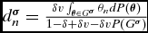 $d_{n}^{\boldsymbol{\sigma }}=\frac{\delta v\int _{\boldsymbol{ \theta }\in G^{\boldsymbol{\sigma }}}\theta _{n}dP\left( \boldsymbol{\theta } \right) }{1-\delta +\delta v-\delta vP\left( G^{\boldsymbol{\sigma }}\right) }$. Using Assumption 1(A), we conclude that d σ1 ⩽ . . . ⩽ dN σ, with strict inequalities if
 $P\left( G^{ \boldsymbol{\sigma }}\right) >0$. Since d σ1 ⩽ . . . ⩽ dN σ,
 $\boldsymbol{\theta }\left( t\right) +\boldsymbol{d} ^{\sigma }$ also satisfies Assumption 1(A). Since each n votes for R if and only if
 $\theta _{n}\left( t\right) +d_{n}^{\boldsymbol{ \sigma }}\ge 0,$ the same reasoning as in the Static Model section implies that on the path of
 $\boldsymbol{\sigma }$, l(Ω) and r(Ω) as defined in Equations (3) and (4) are pivotal under status quo L and R, respectively. Since l(Ω) ≤ r(Ω), we obtain that a state
 $\boldsymbol{\theta }\in \mathbb {R} ^{N}$ is a gridlock state if and only if in
 $\boldsymbol{\theta }$,
 $\boldsymbol{\sigma }$ prescribes l(Ω) to vote for L and r(Ω) to vote for R, or equivalently, θl(Ω) + d σl(Ω) < 0 ⩽ θr(Ω) + d σr(Ω). From Equation (15), this means that
 $G^{\boldsymbol{\sigma } }=G\left( \Omega ,\boldsymbol{d}^{\boldsymbol{\sigma }}\right) $. Substituting
 $G^{\boldsymbol{\sigma }}=G\left( \Omega ,\boldsymbol{d}^{ \boldsymbol{\sigma }}\right)$ in Equation (18), we obtain
 $d_{n}^{\sigma }=D_{n}\left( G\left( \Omega ,\boldsymbol{d}^{\sigma }\right) ,d_{n}^{\sigma }\right)$.
Now we show that if  $\boldsymbol{d}$solves
 $\boldsymbol{d}=D\left( G\left( \Omega ,\boldsymbol{d}\right) ,\boldsymbol{d}\right)$ and
 $\boldsymbol{ \sigma }^{\boldsymbol{d}}$ is the strategy profile in which each
 $n\in \mathcal {N}$ votes for R if and only if θn(t) + d n ≥ 0, then
 $\boldsymbol{\sigma }^{\boldsymbol{d}}$ is an equilibrium. By construction,
 $\boldsymbol{\sigma }^{\boldsymbol{d}}$ is stationary, so it suffices to show that
 $\boldsymbol{\sigma }^{\boldsymbol{d} }$ prescribes stage-undominated actions to each n for almost all
 $\boldsymbol{\theta }$. As argued in the proof of Step 1, this is the case if
 $\sigma _{n}^{\boldsymbol{d}}$ prescribes n to vote for R if and only if
 $V_{n}^{\boldsymbol{\sigma }^{\boldsymbol{d}}}\left( \boldsymbol{\theta } ,R\right) \ge V_{n}^{\boldsymbol{\sigma }^{\boldsymbol{d}}}\left( \boldsymbol{\theta },L\right)$, or equivalently, if and only if
 $\theta _{n}+d^{\boldsymbol{\sigma }^{\boldsymbol{d}}}\ge 0,$ where
 $V_{n}^{ \boldsymbol{\sigma }^{\boldsymbol{d}}}$ and
 $d_{n}^{\boldsymbol{\sigma }^{ \boldsymbol{d}}}$ are as defined in Step 0. So
 $\boldsymbol{\sigma }^{ \boldsymbol{d}}$ is an equilibrium if
 $\boldsymbol{d}^{\boldsymbol{\sigma }^{ \boldsymbol{d}}}=\boldsymbol{d}$. Below, we establish this equality.
From Equation (16),  $d_{n}=D_{n}\left( G\left( \Omega ,\boldsymbol{d} \right) ,d_{n}\right)$ can be rewritten as
 $d_{n}=\frac{\delta v\int _{ \boldsymbol{\theta }\in G\left( \Omega ,\boldsymbol{d}\right) }\theta _{n}dP\left( \boldsymbol{\theta }\right) }{1-\delta +\delta v-\delta vP\left( G\left( \Omega ,\boldsymbol{d}\right) \right) }$. Using the same argument as the paragraph after Equation (18), the latter equation implies that d 1 ≤ . . . ≤ d N, and thus that a state
 $\boldsymbol{\theta }\in \mathbb {R} ^{N}$ is a gridlock state for
 $\boldsymbol{\sigma }^{\boldsymbol{d}}$ if and only if in state
 $\boldsymbol{\theta }$, l(Ω) votes for L and r(Ω) votes for R, or equivalently, θl(Ω) + d l(Ω) < 0 ≤ θr(Ω) + d r(Ω). Using Equation (15), this means that
 $G^{\boldsymbol{\sigma }^{\boldsymbol{d} }}=G\left( \Omega ,\boldsymbol{d}\right) $. To conclude, note that to derive Equations (17) and (18), we only use the fact that
 $\boldsymbol{\sigma }$ is stationary and independent of the status quo. So Equation (18) also holds for
 $\boldsymbol{\sigma }^{\boldsymbol{d}}$. Substituting
 $G^{\boldsymbol{\sigma } ^{\boldsymbol{d}}}=G\left( \Omega ,\boldsymbol{d}\right)$ in Equation (18), we obtain
 $d_{n}^{\boldsymbol{\sigma }^{\boldsymbol{d} }}=D_{n}\left( G\left( \Omega ,\boldsymbol{d}\right) ,d_{n}^{\boldsymbol{ \sigma }^{\boldsymbol{d}}}\right)$. This equation is linear in
 $d_{n}^{ \boldsymbol{\sigma }^{\boldsymbol{d}}}$. Straightforward algebra shows that its solution is unique. Since by assumption d n is a solution, necessarily
 $d_{n}^{\boldsymbol{\sigma }^{\boldsymbol{d}}}=d_{n}$.
Step 3: Proof of Propositions 2 (i) and 2 (ii). If Ω is quasi-dictatorial, from Equation (15), l(Ω) = r(Ω) implies  $G\left( \Omega , \boldsymbol{d}\right) =\emptyset ,$ so
 $\boldsymbol{d}=\boldsymbol{D}\left( \emptyset ,\boldsymbol{d}\right) =\left( 0,. . .,0\right) $. Suppose now that Ω is not quasi-dictatorial, and let
 $\boldsymbol{d}$ be the distortions of an equilibrium of Γ(Ω). From Equation (15), for all
 $\boldsymbol{\theta }\in G\left( \Omega , \boldsymbol{d}\right)$, θl(Ω) + d l(Ω) < 0 ≤ θr(Ω) + d r(Ω), and from Step 2,
 $\boldsymbol{d}=\boldsymbol{D}\left( G\left( \Omega ,\boldsymbol{d}\right) ,\boldsymbol{d}\right)$, so from Equation (16),
 $$\begin{eqnarray*}
d_{l\left( \Omega \right) }&=&D_{l\left( \Omega \right) }\left( G\left( \Omega ,\boldsymbol{d}\right) ,d_{l\left( \Omega \right) }\right) \le 0\\
&&\le D_{r\left( \Omega \right) }\left( G\left( \Omega ,\boldsymbol{d}\right) ,d_{r\left( \Omega \right) }\right) =d_{r\left( \Omega \right) }.
\end{eqnarray*}$$
If we denote  $T\equiv \left\lbrace \boldsymbol{\theta }\in \mathbb {R} ^{N}:\theta _{l\left( \Omega \right) }<0\text{ and }\theta _{r\left( \Omega \right) }>0\right\rbrace\!,$ the above inequalities imply
 $T\subseteq G\left( \Omega ,\boldsymbol{d}\right) $. Since l(Ω) < r(Ω), Assumption 1(B) implies P(T) > 0, so
 $P\left( G\left( \Omega ,\boldsymbol{d}\right) \right) >0$, and from Step 2, d 1 < . . . < d N, which proves Proposition 2(i).
Using successively the fact that for all  $\boldsymbol{\theta }\in G\left( \Omega ,\boldsymbol{d}\right) ,$ θr(Ω) + d r(Ω) ≥ 0,
 $T\subseteq G\left( \Omega , \boldsymbol{d}\right) ,$d r(Ω) ≥ 0, and P(T) > 0, we have
 $$\begin{eqnarray*}
d_{r\left( \Omega \right) }&=&D_{r\left( \Omega \right) }\left( G\left( \Omega ,\boldsymbol{d}\right) ,d_{r\left( \Omega \right) }\right) \ge \frac{\delta v\int _{T}\left( \theta _{r\left( \Omega \right) }+d_{r\left( \Omega \right) }\right) dP\left( \boldsymbol{\theta }\right) }{1-\delta +\delta v}\\
&&\ge \frac{\delta v\int _{T}\theta _{r\left( \Omega \right) }dP\left( \boldsymbol{ \theta }\right) }{1-\delta +\delta v}>0.
\end{eqnarray*}$$
An analogous reasoning shows that d l(Ω) < 0, which proves Proposition 2(ii). ▪
Parts A and B of the following lemma prove the claim made at the end of the Dynamic Model section that equilibria can be ordered in terms of the degree of strategic polarization of the pivots. Part C will be used to derive comparative statics w.r.t. Ω and v for the least polarized equilibrium (see the proofs of Propositions 4 and 7).
Lemma 1 (multiplicity and polarization)
For any pair of profiles of voting distortions  $\boldsymbol{d},\boldsymbol{d}^{\prime }\in \mathbb {R} ^{N},$ we say that
 $\boldsymbol{d}$ is strictly more polarized than
 $\boldsymbol{d}^{\prime }$ if d l(Ω) < d′l(Ω) and d r(Ω) > d′r(Ω).
(A) For any two distinct equilibria
$\boldsymbol{\sigma }$ and $\boldsymbol{\sigma }^{\prime }$ with distortions $\boldsymbol{d}$ or $\boldsymbol{d}^{\prime }$, respectively, either $\boldsymbol{d}$ is strictly more polarized than $\boldsymbol{d}^{\prime }$, or vice versa.(B) There exists an equilibrium
$\boldsymbol{\sigma }$ whose profile of distortions $\boldsymbol{d}$ is least (most) polarized among all equilibria; that is, for all equilibria $\boldsymbol{\sigma }^{\prime }$ with distortions $\boldsymbol{d}^{\prime },$ if $\boldsymbol{d}^{\prime }\not=\boldsymbol{d}$, then d l(Ω) > d′l(Ω) and d r(Ω) < d′r(Ω) (d l(Ω) < d′l(Ω) and d r(Ω) > d′r(Ω)).(C) If there exists
$\boldsymbol{d}^{o}\in \mathbb {R} ^{N}$ s.t. $d_{l\left( \Omega \right) }^{o}\le D_{l\left( \Omega \right) }\left( G\left( \Omega ,\boldsymbol{d}^{o}\right) ,d_{l\left( \Omega \right) }^{o}\right)$ and $d_{r\left( \Omega \right) }^{o}\ge D_{r\left( \Omega \right) }\left( G\left( \Omega ,\boldsymbol{d}^{o}\right) ,\break d_{r\left( \Omega \right) }^{o}\right)$ with one inequality strict, then there exists an equilibrium $\boldsymbol{\sigma }$ whose distortions $\boldsymbol{d}$ are strictly less polarized than $\boldsymbol{d}^{o}$.


Proof. In this proof, we omit Ω from the notations. Using Notation 1, Proposition 3 states that equilibrium distortions are given by the fixed points of  $\boldsymbol{d}\rightarrow \boldsymbol{D}\left( G\left( \boldsymbol{d}\right) ,\boldsymbol{d}\right)$. As explained in Remark 1, there is a one-to-one mapping between the set of these fixed points, and the fixed points for the pivots only:
 $\left( d_{l},d_{r}\right) \rightarrow \left( D_{l}\left( G\left( \boldsymbol{d}\right) ,d_{r}\right) ,D_{l}\left( G\left( \boldsymbol{d}\right) ,d_{r}\right) \right) $. Moreover, the gridlock
 $G\left( \boldsymbol{d}\right)$ is determined solely by the distortions of the pivots (d l, d r). For the rest of the proof, we denote the fixed-point mapping restricted only to the pivots by (d l, d r) → (Δl, Δr)(d l, d r). That is, for all n ∈ {l, r} and
 $d_{l},d_{r}\in \mathbb {R} ,$
 $$\begin{eqnarray}
\Delta _{n}\left( d_{l},d_{r}\right) &\equiv& D_{n}\left( G\left( \boldsymbol{d }\right) ,d_{n}\right) =\frac{\delta v}{1-\delta +\delta v}\nonumber\\
&&\times\int _{\theta _{l}+d_{l}<0\le \theta _{r}+d_{r}}\left( \theta _{n}+d_{n}\right) dP\left( \boldsymbol{\theta }\right).
\end{eqnarray}$$
Proof of Part A. From what precedes, if  $\boldsymbol{d}^{\ast }$ and
 $\boldsymbol{d}^{\ast \ast }$ are the profiles of voting distortions of two distinct equilibria, then (d*l, dr*) and (d**l, dr**) are two distinct fixed points of (Δl, Δr). Suppose d*l ≠ dl**; the proof in the case d*r ≠ dr** is analogous. Suppose w.l.o.g. that d**l < dl*. We need to prove d**r > dr*. From Equation ( 19),
 $$\begin{eqnarray*}
\frac{\partial \Delta _{r}\left( d_{l},d_{r}\right) }{\partial d_{r}}&=&\frac{ \delta v}{1-\delta +\delta v}P\left( \boldsymbol{\theta }\in \mathbb {R} ^{N}:\theta _{l}+d_{l}<0\le \theta _{r}+d_{r}\right)\nonumber\\
&& \in \left[ 0,\frac{ \delta v}{1-\delta +\delta v}\right] ,
\end{eqnarray*}$$
so d r → Δr(d l, d r) is a weakly increasing contraction, and hence d*r and d**r are its unique fixed points for dl = d*l and dl = d**l, respectively. Theorem 2 in Villas-Boas (Reference Villas-Boas1997) states that if Δr(d l, d r) is strictly decreasing in d l, the fixed point of d r → Δr(d l, d r) is strictly decreasing in d l, and thus that d**r > dr*, as needed. So it suffices to show Δr(d**l, dr) > Δr(d*l, dr) for all dr ⩾ d*l (from Proposition 2 all fixed points of Δ are such that d l ≤ d r). From Assumption 1(A), for all dr ⩾ d*l, 0 ⩽ θl + d*l implies 0 < θr + d r almost surely, so from Equation (19),
 $$\begin{eqnarray*}
&&\Delta _{r}\left( d_{l}^{\ast \ast },d_{r}\right) -\Delta _{r}\left( d_{l}^{\ast },d_{r}\right) =\frac{\delta v}{1-\delta +\delta v}\\
&&\times \int \nolimits _{\theta _{l}\in \left[ -d_{l}^{\ast },-d_{l}^{\ast \ast }\right) }\left( \theta _{r}+d_{r}\right) dP\left( \boldsymbol{\theta } \right) >0,
\end{eqnarray*}$$
where the strict inequality comes from d**l < dl* and θl(t) having full support.
Proof of Part B. This proof relies on establishing that the conditions of Tarsky’s fixed point theorem hold.
Step B1: Let  $B\equiv \frac{\delta v}{1-\delta }\max \left\lbrace E\left[ \left|\theta _{l}\left( t\right) \right|,\left|\theta _{r}\left( t\right) \right|\right] \right\rbrace $. All fixed points of (d l, d r) → (Δl, Δr)(d l, d r) are in [− B, B]2, and (Δl, Δr)([− B, B]2)⊆[− B, B]2.
From Equation (19), for any n ∈ {l, r},  $\left|d_{n}\right|=\left|\Delta _{n}\left( d_{l},d_{r}\right) \right|\le \frac{\delta v}{1-\delta +\delta v}\left( E\left[ \left|\theta _{n}\left( t\right) \right|\right] +\left|d_{n}\right|\right) $. Isolating |d n|, we obtain |d n| ≤ B, which proves the first claim of Step B1. To prove the second claim, let (d l, d r) ∈ [− B, B]2 and n ∈ {l, r}, then
 $$\begin{eqnarray*}
&&\left|\Delta _{n}\left( d_{l},d_{r}\right) \right|\\
&&\le \frac{ \delta v}{1-\delta +\delta v}\left( \max \left\lbrace E\left[ \left|\theta _{l}\left( t\right) \right|\right] ,E\left[ \left|\theta _{r}\left( t\right) \right|\right] \right\rbrace +B\right) =B.
\end{eqnarray*}$$
Step B2: Consider the partial order ⊵ on [− B, B]2 defined by: for all (d l, d r) ∈ [− B, B]2, (d′l, dr′) ⊵ (dl, dr) if d′l ⩽ dl and d′r ⩾ dr .Footnote 27 Then [− B, B]2 is a complete lattice for ⊵ ,Footnote 28 and (Δl, Δr) is monotone for ⊵ .Footnote 29
That ⊵ is a partial order on [−B, B]2 is immediate and omitted for brevity. To see why [−B, B]2 is a complete lattice for ⊵, note that the least upper bound of a subset S of [−B, B]2 is given by  $\bar{d}_{l}=\sup \left\lbrace d_{l}:\left( d_{l},d_{r}\right) \in S\right\rbrace$ and
 $\bar{d} _{r}=\inf \left\lbrace d_{r}:\left( d_{l},d_{r}\right) \in S\right\rbrace ,$ and
 $\left( \bar{d}_{l},\bar{d}_{r}\right) \in \left[ -B,B\right] ^{2},$ as needed. The proof for the greatest lower bound is analogous.
We now prove monotonicity of (Δl, Δr). For all d l, d r, let  $G\left( d_{l},d_{r}\right) \equiv \left\lbrace \boldsymbol{\theta }\in \mathbb {R} ^{N}:\theta _{l}+d_{l}<0\le \theta _{r}+d_{r}\right\rbrace$. Then if (d′l, dr′)⊵(dl, dr), G(dl, dr)⊆G(d′l, d′r), so from Equation (19),
 $$\begin{eqnarray*}
&&\Delta _{r}\left( d_{l}^{\prime },d_{r}^{\prime }\right) -\Delta _{r}\left( d_{l},d_{r}\right) =\frac{\delta v}{1-\delta +\delta v}\\
&&\times\left[\!\!\int \limits _{G\left( d_{l},d_{r}\right) }\left( d_{r}^{\prime }-d_{r}\right) dP\left( \boldsymbol{\theta }\right)\! +\!\!\int \limits _{G\left( d_{l}^{\prime },d_{r}^{\prime }\right) \setminus G\left( d_{l},d_{r}\right) }\left( \theta _{r}+d_{r}^{\prime }\right) dP\left( \boldsymbol{\theta }\right) \right] .
\end{eqnarray*}$$
The integrands of the two integrals on the right-hand side of the above equation are nonnegative on their domains of integration, so Δr(d′l, d′r) ⩾ Δr(dl, dr). An analogous argument shows that Δl(d′l, d′r) ⩽ Δl(dl, dr).
Step B3: Conclusion
From Steps B1 and B2, all the fixed points of (Δl, Δr) are in the complete lattice [−B, B]2, and (Δl, Δr) is monotone from [−B, B]2 to [−B, B]2 for ⊵. Tarsky’s theorem implies then that (Δl, Δr) has a least (greatest) fixed point (d*l, dr*) for ⊵. Let  $\boldsymbol{d}^{\ast }$ denote the corresponding fixed point of
 $\boldsymbol{d}\rightarrow D\left( G\left( \Omega , \boldsymbol{d}\right) ,\boldsymbol{d}\right) $. By Proposition 3, there exists an equilibrium
 $\boldsymbol{\sigma }$ corresponding to
 $\boldsymbol{d}^{\ast }\boldsymbol{.}$ By construction, d*l ⩾ ( ⩽)dl and d*r ⩽ (⩾)dr for any other equilibrium distortions
 $\boldsymbol{d} \ne \boldsymbol{d}^{\ast }$. By Part A, if
 $\boldsymbol{d}\ne \boldsymbol{d }^{\ast },$ then
 $\boldsymbol{d}$ is strictly more polarized than
 $\boldsymbol{d}^{\ast }$ or vice versa; hence by what precedes, d*l > dl and d*r < dr (d*l < dl and d*r > dr) and hence
 $\boldsymbol{d}^{\ast }$ is the least (most) polarized equilibrium.
Proof of Part C.
Suppose  $\boldsymbol{d}^{o}$ satisfies the conditions of Part C. Consider the (constant) mapping f o defined by: for all
 $\left( d_{l},d_{r}\right) \in \mathbb {R} ^{2},$fo(dl, dr) = (dol, dor). Then (dol, dr o) is the unique fixed point of f o and by assumption, (dol, dr o)⊵(Δ1, Δ2)(dol, dor). Theorem 5 in Villas-Boas (Reference Villas-Boas1997) applied to the mappings f o and (Δ1, Δ2) implies that (Δ1, Δ2) admits a fixed point (d*l, dr*) such that (dol, dr o)⊵(d*l, dr*). By assumption,
 $d_{l}^{o}<D_{l}\left( G\left( \boldsymbol{d} ^{o}\right) ,d_{l}^{o}\right)$ or
 $d_{r}^{o}>D_{r}\left( G\left( \boldsymbol{d}^{o}\right) ,d_{r}^{o}\right) $. Suppose the former, the latter case is analogous. Using Step B2 and (dol, dr o)⊵(d*l, dr*), we have
 $$\begin{equation}
d_{l}^{o}<\Delta _{l}\left( d_{l}^{o},d_{r}^{o}\right) \le \Delta _{l}\left( d_{l}^{\ast },d_{r}^{\ast }\right) =d_{l}^{\ast }.
\end{equation}$$
As shown in the proof of Part A, Δr is strictly increasing in d l, so using successively (dol, dr o)⊵(Δl, Δr)(dol, dor), Equation (19), and Step B2,
 $$\begin{equation}
d_{r}^{o}\ge \Delta _{r}\left( d_{l}^{o},d_{r}^{o}\right) >\Delta _{r}\left( d_{l}^{\ast },d_{r}^{o}\right) \ge \Delta _{r}\left( d_{l}^{\ast },d_{r}^{\ast }\right) =d_{r}^{\ast }.
\end{equation}$$
Since (d*l, dr*) is a fixed point of (Δl, Δr), from what precedes, there exists a corresponding fixed point  $\boldsymbol{d}^{\ast }$ of
 $\boldsymbol{d} \rightarrow D\left( G\left( \Omega ,\boldsymbol{d}\right) ,\boldsymbol{d} \right)$ and by Proposition 3, there exists an equilibrium with distortion
 $\boldsymbol{d}^{\ast }$. From Equations (20) and (21),
 $\boldsymbol{d}^{\ast }$ is strictly less polarized than
 $\boldsymbol{d}^{o}$. ▪
Proof of Proposition 4. Let (l, r) and (l′, r′) denote pivots for Ω and Ω′, respectively.
Step 1: l′ ≤ l ≤ r ≤ r′.
From Equation (3), {l + 1, . . ., N}∉ΩL so Definition 2 implies {l + 1, . . ., N}∉Ω′L. From Equation (3) again, {l′, . . ., N} ∈ Ω′L so Assumption 2(A) implies l + 1 > l′, and therefore l ≥ l′. An analogous reasoning shows that r ≤ r′.
Step 2: The four inner inequalities in Equation (13) hold. If l = l′ and r = r′, then the two outer inequalities in Equation (13) and the inequality Equation (14) hold with equality. The four inner inequalities in Equation (13) follow directly from Step 1 and the fact stated in Proposition 2 that distortions are ordered. If l = l′ and r = r′, then the equilibria of Γ(Ω) and Γ(Ω′) are the same, which proves the remaining claims in Step 2.
Step 3: If (l, r) ≠ (l′, r′), then dl(Ω) > d l′(Ω′) and dr(Ω) < d r′(Ω′).
Suppose r < r′, the proof in the case l > l′ is analogous. Let  $\boldsymbol{d}^{o}\in \mathbb {R} ^{N}$ be such that dol = d l′(Ω′) and dor = d r′(Ω′). From Equation (15) and Assumption 2(A), up to P-negligible events, θl(t) + d l′(Ω′) < 0 ⩽ θr(t) + d r′(Ω′) implies θl′(t) + d l′(Ω′) < 0 ⩽ θr′(t) + d r′(Ω′) so
 $$\begin{eqnarray}
G\left( \Omega ,\boldsymbol{d}^{o}\right) &=&\left\lbrace \boldsymbol{\theta }\in \mathbb {R} ^{N}:\theta _{l}+d_{l^{\prime }}\left( \Omega ^{\prime }\right) <0\le \theta _{r}+d_{r^{\prime }}\left( \Omega ^{\prime }\right) \right\rbrace \nonumber\\
&& \subseteq G\left( \Omega ^{\prime },\boldsymbol{d}\left( \Omega ^{\prime }\right) \right) .
\end{eqnarray}$$
Using successively the definition of  $\boldsymbol{d}^{o}$, the fact that
 $\boldsymbol{d}\left( \Omega ^{\prime }\right)$ is an equilibrium of Γ(Ω′), and
 $G\left( \Omega ,\boldsymbol{d} ^{o}\right) \subseteq G\left( \Omega ^{\prime },\boldsymbol{d}\left( \Omega ^{\prime }\right) \right) ,$ we have
 $$\begin{eqnarray}
&&d_{r}^{o}-D_{r}\left( G\left( \Omega ,\boldsymbol{d}^{o}\right) ,d_{r}^{o}\right) \nonumber \\
&&\quad =d_{r^{\prime }}\left( \Omega ^{\prime }\right) -D_{r}\left( G\left( \Omega ,\boldsymbol{d}^{o}\right) ,d_{r^{\prime }}\left( \Omega ^{\prime }\right) \right) \nonumber \\
&&\quad =D_{r^{\prime }}\left( G\left( \Omega ^{\prime },\boldsymbol{d}\left( \Omega ^{\prime }\right) \right) ,d_{r^{\prime }}\left( \Omega ^{\prime }\right) \right)\! -\!D_{r}\left( G\left( \Omega ,\boldsymbol{d}^{o}\right) ,d_{r^{\prime }}\left( \Omega ^{\prime }\right) \right) \nonumber \\
&&\quad=\frac{\delta v}{1-\delta +\delta v}\nonumber\\
&&\quad \times\left[ \int \limits _{G\left( \Omega ^{\prime },\boldsymbol{d}\left( \Omega ^{\prime }\right) \right) \setminus G\left( \Omega ,\boldsymbol{d}^{o}\right) }\left[ \theta _{r^{\prime }}+d_{r^{\prime }}\left( \Omega ^{\prime }\right) \right] dP\left( \boldsymbol{\theta }\right)\right.\nonumber\\
&&\qquad\qquad\left. +\,\int \limits _{G\left( \Omega ,\boldsymbol{d} ^{o}\right) }\left[ \theta _{r^{\prime }}-\theta _{r}\right] dP\left( \boldsymbol{\theta }\right) \right] .
\end{eqnarray}$$
By definition of  $G\left( \Omega ^{\prime },\boldsymbol{d}\left( \Omega ^{\prime }\right) \right) ,$ the first integral in Equation (23) is nonnegative. Since r < r′, Step 1 implies that l′ < r′ so from Proposition 2, d l′(Ω′) < d r′(Ω′). Since θr(t) has full support, the following set
 $T\equiv \left\lbrace \boldsymbol{\theta }\in \mathbb {R} ^{N}:\theta _{r}+d_{l^{\prime }}\left( \Omega ^{\prime }\right) <0\le \theta _{r}+d_{r^{\prime }}\left( \Omega ^{\prime }\right) \right\rbrace$ has positive probability. Since θl(t) ≤ θr(t) with probability 1,
 $P\left( G\left( \Omega , \boldsymbol{d}^{o}\right) \right) \ge P\left( T\right) ,$ so
 $P\left( G\left( \Omega ,\boldsymbol{d}^{o}\right) \right) >0$. Together with r < r′ and Assumption 2(A), this implies that the second integral in Equation (23) is strictly positive, so
 $d_{r}^{o}>D_{r}\left( G\left( \Omega ,\boldsymbol{d} ^{o}\right) ,d_{r}^{o}\right) $. An analogous argument shows that
 $d_{l}^{o}\le D_{l}\left( G\left( \Omega ,\boldsymbol{d}^{o}\right) ,d_{l}^{o}\right) $. Lemma 1C implies then that there exists an equilibrium
 $\boldsymbol{\sigma }$ of Γ(Ω) whose distortion
 $\boldsymbol{d}$ are strictly less polarized than
 $\boldsymbol{d}^{o}$, so the least polarized equilibrium distortions
 $\boldsymbol{d}\left( \Omega \right)$ must also be strictly less polarized than
 $\boldsymbol{d}^{o}$.
Step 4: If (l, r) ≠ (l′, r′), then the two outer inequalities in Equation (13) hold strictly.
Assumption 1(A), and Steps 1 and 3 imply that up to P -negligible sets,  $G\left( \Omega ,\boldsymbol{d}\left( \Omega \right) \right) \subseteq G\left( \Omega ^{\prime },\boldsymbol{d}\left( \Omega ^{\prime }\right) \right) $. Using Proposition 3 and the latter inclusion, we get that for all
 $n\in \mathcal {N},$
 $$\begin{eqnarray*}
&&d_{n}\left( \Omega ^{\prime }\right) -d_{n}\left( \Omega \right) =D_{n}\left( G\left( \Omega ^{\prime },\boldsymbol{d}\left( \Omega ^{\prime }\right) \right) ,d_{n}\left( \Omega ^{\prime }\right) \right)\\
&&\quad -D_{n}\left( G\left( \Omega ,\boldsymbol{d}\left( \Omega \right) \right) ,d_{n}\left( \Omega \right) \right) \\
&&\quad =\frac{\delta v}{1-\delta +\delta v}\left\lbrace \int \limits _{G\left( \Omega , \boldsymbol{d}\left( \Omega \right) \right) }\left[ d_{n}\left( \Omega ^{\prime }\right) -d_{n}\left( \Omega \right) \right] dP\left( \boldsymbol{ \theta }\right)\right.\\
&&\qquad\qquad\qquad\left. +\int \limits _{G\left( \Omega ^{\prime },\boldsymbol{d}\left( \Omega ^{\prime }\right) \right) \setminus G\left( \Omega ,\boldsymbol{d} \left( \Omega \right) \right) }\left[ \theta _{n}+d_{n}\left( \Omega ^{\prime }\right) \right] dP\left( \boldsymbol{\theta }\right) \right\rbrace .
\end{eqnarray*}$$
Isolating d n(Ω′) − d n(Ω) in, we obtain
 $$\begin{equation}
d_{n}\left( \Omega ^{\prime }\right) -d_{n}\left( \Omega \right) =\frac{ \int _{G\left( \Omega ^{\prime },\boldsymbol{d}\left( \Omega ^{\prime }\right) \right) \setminus G\left( \Omega ,\boldsymbol{d}\left( \Omega \right) \right) }\left[ \theta _{n}+d_{n}\left( \Omega ^{\prime }\right) \right] dP\left( \boldsymbol{\theta }\right) }{\frac{1-\delta +\delta v}{ 1-\delta +\delta v\left( 1-P\left( G\left( \Omega ,d\left( \Omega \right) \right) \right) \right) }}.
\end{equation}$$
For n = r′, the function inside the integral in Equation (24) is nonnegative on  $G\left( \Omega ^{\prime },\boldsymbol{d} \left( \Omega ^{\prime }\right) \right)$. So to prove that d r′(Ω′) > d r′(Ω), it suffices to prove that θr′ + d r′(Ω′) > 0 for a subset of
 $G\left( \Omega ^{\prime },\boldsymbol{d}\left( \Omega ^{\prime }\right) \right) \setminus G\left( \Omega ,\boldsymbol{d}\left( \Omega \right) \right)$ that has positive probability. Let
 $T^{\prime }\equiv \left\lbrace \boldsymbol{\theta }\in \mathbb {R} ^{N}:\theta _{r^{\prime }}+d_{r}\left( \Omega \right) <0<\theta _{r^{\prime }}+d_{r^{\prime }}\left( \Omega ^{\prime }\right) \right\rbrace $. Since θn(t) has full support, Step 3 implies P(T′) > 0. Moreover, from Step 1, r′ ≥ r ≥ l′ and dr(Ω) ⩾ 0 ⩾ d l′(Ω′), so Assumption 1(A) implies that for almost all
 $\boldsymbol{\theta }\in T^{\prime },$0 > θr′ + dr(Ω) ⩾ θr + dr(Ω) ⩾ θl′ + d l′(Ω′). These inequalities imply θr + d r(Ω) < 0, and so
 $\boldsymbol{\theta }\notin G\left( \Omega ,d\left( \Omega \right) \right)$ for almost all
 $\boldsymbol{\theta }\in T^{\prime }$. They also imply θl′ + d l′(Ω′) < 0, and by definition of T′, 0 < θr′ + d r′(Ω′), so
 $\boldsymbol{\theta }\in G\left( \Omega ^{\prime },d\left( \Omega ^{\prime }\right) \right) $. So up to a P-negligible set, T′ is a subset of
 $G\left( \Omega ^{\prime },\boldsymbol{d}\left( \Omega ^{\prime }\right) \right) \setminus G\left( \Omega ,\boldsymbol{d}\left( \Omega \right) \right) ,$ as needed. A symmetric argument shows d l′(Ω′) < d l′(Ω).
Step 5: If l ≠ l′ or r ≠ r′, Equation (14) holds strictly with probability 1.
From Equation (24),
 $$\begin{eqnarray*}
&&d_{n}\left( \Omega ^{\prime }\right) -d_{n}\left( \Omega \right) -\left( d_{m}\left( \Omega ^{\prime }\right) -d_{m}\left( \Omega \right) \right) \\
&&\quad =\frac{\int _{G\left( \Omega ^{\prime },\boldsymbol{d}\left( \Omega ^{\prime }\right) \right) \setminus G\left( \Omega ,\boldsymbol{d}\left( \Omega \right) \right) }\left[ \theta _{n}+d_{n}\left( \Omega ^{\prime }\right) -\left( \theta _{m}+d_{m}\left( \Omega ^{\prime }\right) \right) \right] dP\left( \boldsymbol{\theta }\right) }{\frac{1-\delta +\delta v}{ 1-\delta +\delta v\left( 1-P\left( G\left( \Omega ,d\left( \Omega \right) \right) \right) \right) }}.
\end{eqnarray*}$$
As argued in Step 4,  $P\left( G\left( \Omega ^{\prime },\boldsymbol{d}\left( \Omega ^{\prime }\right) \right) \setminus G\left( \Omega ,\boldsymbol{d} \left( \Omega \right) \right) \right) >0$. If n > m, then with probability 1, θn + d n(Ω′) > θm + d m(Ω′), so the above equation implies d n(Ω′) − d n(Ω) > d m(Ω′) − d m(Ω) and hence that Equation (14) holds strictly. An analogous argument holds for n < m. ▪
Proof of Proposition 5. Since for all  $n\in \mathcal {N},$
 $\theta _{n}\left( t\right) =\bar{\theta } _{n}+\varepsilon \left( t\right)$ with
 $\sum _{n\in \mathcal {N}}\bar{\theta } _{n}=0,$Equation (10) can be rewritten as
 $$\begin{equation}
\frac{1}{N}\sum \nolimits _{n\in \mathcal {N}}d_{n}=\frac{\delta }{1-\delta F\left( G\right) }\int _{-\bar{\theta }_{r}-d_{r}}^{-\bar{\theta } _{l}-d_{l}}\varepsilon dF\left( \varepsilon \right) ,
\end{equation}$$
where  $G=\left( -\bar{\theta }_{l}-d_{l},-\bar{\theta }_{r}-d_{r}\right)$. Suppose, by contradiction, that
 $\frac{1}{N}\sum _{n\in \mathcal {N}}d_{n}\ge 0,$ which requires
 $\int _{-\bar{\theta }_{r}-d_{r}}^{-\bar{\theta } _{l}-d_{l}}\varepsilon dF\left( \varepsilon \right) \ge 0$. By symmetry of F, this implies that the interval of integration
 $\left( -\bar{\theta } _{l}-d_{l},-\bar{\theta }_{r}-d_{r}\right)$ must be skewed to the right, that is,
 $-\bar{\theta }_{l}-d_{l}-\bar{\theta }_{r}-d_{r}\ge 0$. Since
 $\left( \bar{\theta }_{n}\right) _{n\in \mathcal {N}}$ is symmetrically distributed around 0, and since Ω is biased in favor of R,
 $\bar{ \theta }_{r}+\bar{\theta }_{l}>0$. The last two inequalities imply that d r + d l < 0. Using, successively, Equation (9),
 $\bar{\theta }_{r}+ \bar{\theta }_{l}>0$, and
 $\int _{-\bar{\theta }_{r}-d_{r}}^{-\bar{\theta } _{l}-d_{l}}\varepsilon dF\left( \varepsilon \right) \ge 0,$ we obtain a contradiction:
 $$\begin{eqnarray*}
d_{l}+d_{r}&=&\frac{\delta \int _{-\bar{\theta }_{r}-d_{r}}^{-\bar{\theta } _{l}-d_{l}}\left( \bar{\theta }_{l}+\bar{\theta }_{r}+2\varepsilon \right) dF\left( \varepsilon \right) }{1-\delta F\left( G\right) }\\
&&\ge \frac{\delta \int _{-\bar{\theta }_{r}-d_{r}}^{-\bar{\theta }_{l}-d_{l}}2\varepsilon dF\left( \varepsilon \right) }{1-\delta F\left( G\right) }\ge 0.
\end{eqnarray*}$$
▪
Proof of Proposition 6. Step 1: Let σ be an equilibrium of Γ(Ω) , and let  $\boldsymbol{\sigma }^{\prime }$be strategy profile of Γ(Ω′) such that for any
 $\boldsymbol{\theta }\in \mathbb {R} ^{N}$and q ∈ {L, R} , if status quo q stays in place in state
 $\boldsymbol{\theta }$on the path of
 $\boldsymbol{\sigma }$in Γ(Ω) , then it also stays in place in that state on the path of
 $\boldsymbol{\sigma } ^{\prime }$in Γ(Ω′). Suppose further that for all q ∈ {L, R}, there exists a positive probability set of states in which status quo q stays in place on the path of
 $\boldsymbol{\sigma }^{\prime }$in Γ(Ω′) and all policy makers n ∈ {l(Ω), . . ., r(Ω)} get a strictly greater continuation payoff from implementing the other policy, given continuation play
 $\boldsymbol{\sigma }$in Γ(Ω). Then all policy makers n ∈ {l(Ω), . . ., r(Ω)} get a strictly greater expected discounted payoff from
 $\boldsymbol{\sigma }$in Γ(Ω) than from
 $\boldsymbol{ \sigma }^{\prime }$in Γ(Ω′).
For all  $\tau \in \mathbb {N} ,$ let Γτ be the game that is defined as Γ(Ω) except that in periods 0, . . ., τ − 1, the set of winning coalitions is Ω′ and in all periods t ≥ τ, it is Ω; let
 $\boldsymbol{\sigma }^{\tau }$ be the strategy profile of Γτ in which players play
 $\boldsymbol{\sigma }^{\prime }$ in periods 0, . . ., τ − 1 and play
 $\boldsymbol{\sigma }$ in all periods t ≥ τ. Let us first show that for all
 $\tau \in \mathbb {N}$, all policy makers n ∈ {l(Ω), . . ., r(Ω)} strictly prefer playing
 $\boldsymbol{\sigma } ^{\tau }$ in the game Γτ to playing
 $\boldsymbol{\sigma } ^{\tau +1}$ in the game Γτ + 1. To see this, note that by construction, the games Γτ and Γτ + 1 differ only in period τ, and in that period, they coincide with Γ(Ω) and Γ(Ω′), respectively. Likewise,
 $\boldsymbol{\sigma }^{\tau }$ and
 $\boldsymbol{ \sigma }^{\tau +1}$ differ only in period τ, and in that period, they coincide with
 $\boldsymbol{\sigma }$ and
 $\boldsymbol{\sigma }^{\prime }$, respectively. So the path of
 $\boldsymbol{\sigma }^{\tau }$ in Γτ differ from the path of
 $\boldsymbol{\sigma }^{\tau +1}$ in Γτ + 1 only when the realization of
 $\boldsymbol{\theta }\left( \tau \right)$ and q(τ) is such that in this state and status quo,
 $\boldsymbol{\sigma }$ and
 $\boldsymbol{\sigma }^{\prime }$ implement different policies in Γ(Ω) and Γ(Ω′), respectively. By assumption, for any such realization of
 $\boldsymbol{\theta }\left( \tau \right)$, q(τ) stays in place on the path of
 $\boldsymbol{\sigma }^{\tau +1}$ in Γτ + 1, whereas the other policy x is implemented on the path of
 $\boldsymbol{\sigma }^{\tau }$ in Γτ. Since
 $\boldsymbol{ \sigma }$ is an equilibrium, this means that for any such realization of
 $\boldsymbol{\theta }\left( \tau \right)$,
 $\boldsymbol{\sigma }$ prescribes all n ∈ {l(Ω), . . ., r(Ω)} to vote for x, and thus that all such n weakly prefer implementing x to implementing q(τ), given continuation play
 $\boldsymbol{\sigma }$ in Γ(Ω). Moreover, by assumption, this preference is strict for a positive probability set of such
 $\boldsymbol{\theta }\left( \tau \right)$. Since from period τ + 1 onward, Γτ and Γτ + 1 coincide with Γ(Ω), and
 $\boldsymbol{\sigma }^{\tau }$ and
 $\boldsymbol{ \sigma }^{\tau +1}$ coincide with
 $\boldsymbol{\sigma },$ this implies that ex-ante, all n ∈ {l(Ω), . . ., r(Ω)} strictly prefer playing
 $\boldsymbol{\sigma }^{\tau }$ in Γτ to playing
 $\boldsymbol{\sigma }^{\tau +1}$ in Γτ + 1. To conclude, note that by transitivity, all n ∈ {l(Ω), . . ., r(Ω)} strictly prefer
 $\boldsymbol{\sigma }^{0}=\boldsymbol{\sigma }$ in Γ0 = Γ(Ω) to
 $\boldsymbol{\sigma }^{\tau }$ in Γτ for all τ > 0, so by continuity, they strictly prefer
 $\boldsymbol{\sigma }$ in Γ(Ω) to
 $\lim _{\tau \rightarrow \infty }\boldsymbol{\sigma }^{\tau }=\boldsymbol{\sigma } ^{\prime }$ in limτ → ∞Γτ = Γ(Ω′).
Step 2: Proof of the first claim of Proposition 6.
Let  $\boldsymbol{\sigma }$ and
 $\boldsymbol{\sigma }^{\prime }$ denote the equilibria of Γ(Ω) with distortions
 $\boldsymbol{d }$ and
 $\boldsymbol{d}^{\prime },$ respectively. Then from Equation (8), the set of gridlock states is greater in the inclusion sense for
 $\boldsymbol{\sigma }^{\prime }$ than for
 $\boldsymbol{\sigma }$. Moreover, the probability that
 $\boldsymbol{\theta }\left( t\right)$ is such that status quo L stays in place on the path of
 $\boldsymbol{\sigma }^{\prime }$, but all policy makers n ∈ {l(Ω), . . ., r(Ω)} strictly prefer to implement R given continuation play
 $\boldsymbol{\sigma }$ in Γ(Ω) is given by
 $\Pr \left( \theta _{l\left( \Omega \right) }\left( t\right) +d_{l\left( \Omega \right) }^{\prime }<0<\theta _{l\left( \Omega \right) }\left( t\right) +d_{l\left( \Omega \right) }\right)$. Since
 $\boldsymbol{d} ^{\prime }$ is strictly more polarized than
 $\boldsymbol{d}$, d′l(Ω) < d l(Ω) so our assumption that θl(Ω)(t) has full support imply that this probability is strictly positive. An analogous argument shows that the probability of the symmetric event for status quo R is also strictly positive. Step 1 implies then that all n ∈ {l(Ω), . . ., r(Ω)} strictly prefer
 $\boldsymbol{ \sigma }$ to
 $\boldsymbol{\sigma }^{\prime }$ in Γ(Ω).
Step 3: Proof of the second claim of Proposition 6.
Let  $\boldsymbol{\sigma }$ and
 $\boldsymbol{\sigma }^{\prime }$ denote the least polarized equilibria of Γ(Ω) and Γ(Ω′), respectively. Since Ω′ requires a greater consensus than Ω, Proposition 4 implies that the least polarized equilibrium of Γ(Ω) is less polarized, and its set of gridlock states is smaller in the inclusion sense than the least polarized equilibrium of Γ(Ω′). Moreover, the probability that
 $\boldsymbol{\theta }\left( t\right)$ is such that status quo L stays in place on the path of
 $\boldsymbol{\sigma }^{\prime }$ in Γ(Ω′), but all policy makers n ∈ {l(Ω), . . ., r(Ω)} strictly prefer to implement R given continuation play
 $\boldsymbol{\sigma }$ in Γ(Ω) is given by
 $\Pr \left( \theta _{l\left( \Omega ^{\prime }\right) }\left( t\right) +d_{l\left( \Omega ^{\prime }\right) }\left( \Omega ^{\prime }\right) <0<\theta _{l\left( \Omega \right) }\left( t\right) +d_{l\left( \Omega \right) }\left( \Omega \right) \right) $. Since l(Ω′) ≤ l(Ω) (see Step 1 of the proof of Proposition 4), Assumption 1(A) implies that this probability is no smaller than
 $\Pr \left( \theta _{l\left( \Omega \right) }\left( t\right) +d_{l\left( \Omega ^{\prime }\right) }\left( \Omega ^{\prime }\right) <0<\theta _{l\left( \Omega \right) }\left( t\right) +d_{l\left( \Omega \right) }\left( \Omega \right) \right)$. Since (l(Ω), r(Ω)) ≠ (l(Ω′), r(Ω′)), Proposition 4 implies that d l(Ω′)(Ω′) < d l(Ω)(Ω), so our assumption that θl(Ω)(t) has full support imply the latter probability is strictly positive. An analogous argument shows the probability of the symmetric event for status quo R is also strictly positive. Step 1 implies that all n ∈ {l(Ω), . . ., r(Ω)} strictly prefer
 $\boldsymbol{ \sigma }$ in Γ(Ω) to
 $\boldsymbol{\sigma } ^{\prime }$ in Γ(Ω′). ▪
Proof of Proposition 7. When v = 0, from Equation (16),  $\boldsymbol{D}$ is always equal to
 $\boldsymbol{0},$ so from Proposition 3, the unique equilibrium profile of distortions is
 $\boldsymbol{d}=\boldsymbol{0}$. Suppose now 0 < v < v′ ≤ 1, and let
 $\boldsymbol{D}$ and
 $\boldsymbol{D}^{\prime }$ be the function defined in Equation (16) for v and v′, respectively. Since
 $\frac{\delta v}{1-\delta +\delta v}$ is strictly increasing in v and d′r(Ω) > 0, we have
 $d_{r\left( \Omega \right) }^{\prime }=D_{r\left( \Omega \right) }^{\prime }\left( G\left( \Omega ,\boldsymbol{d}^{\prime }\right) ,d_{r\left( \Omega \right) }^{\prime }\right) >D_{r\left( \Omega \right) }\left( G\left( \Omega ,\boldsymbol{d}^{\prime }\right) ,d_{r\left( \Omega \right) }^{\prime }\right)$. An analogous reasoning implies that
 $d_{l\left( \Omega \right) }^{\prime }<D_{l\left( \Omega \right) }\left( G\left( \Omega ,\boldsymbol{d}^{\prime }\right) ,d_{l\left( \Omega \right) }^{\prime }\right) $. Lemma 1C implies then that Γ(Ω) has an equilibrium that is strictly less polarized than
 $\boldsymbol{d}^{\prime }$. Since
 $\boldsymbol{d}$ is the least polarized equilibrium, it is also strictly less polarized than
 $\boldsymbol{d}^{\prime }$. ▪
Proof of Proposition 8. Let  $\boldsymbol{\sigma }$ be an equilibrium of the game considered in the Political Turnover section. Since
 $\boldsymbol{\sigma }$ is stationary Markov, in every t,
 $\boldsymbol{\sigma }$ maps the payoff relevant variables
 $\boldsymbol{\theta }\left( t\right) ,$
 $\boldsymbol{e}\left( t\right) ,$s(t) and q(t) into a distribution over votes {L, R}. By assumption, the history up to period t affects the continuation game from t + 1 onward only via q(t + 1) and s(t). So let
 $W_{c}^{\boldsymbol{\sigma }}\left( s,q\right)$ denote the continuation payoff for candidate
 $c\in \mathcal {N}$ from period t + 1 conditional on q(t + 1) = q, on s(t) = s ∈ S, and on continuation play
 $\boldsymbol{\sigma }$. Stage undomination (together with our tie-breaking rule) implies that in t,
 $\boldsymbol{ \sigma }$ prescribes c to vote for R if and only if
 $\theta _{c}\left( t\right) +\delta W_{c}^{\boldsymbol{\sigma }}\left( s\left( t\right) ,R\right) \ge \delta W_{c}^{\boldsymbol{\sigma }}\left( s\left( t\right) ,L\right) ,$ which proves the first claim of Proposition 8 for
 $$\begin{equation}
d_{c}^{\boldsymbol{\sigma }}\left( s\right) \equiv \delta \left[ W_{c}^{ \boldsymbol{\sigma }}\left( s,R\right) -W_{c}^{\boldsymbol{\sigma }}\left( s,L\right) \right] .
\end{equation}$$
As argued in the proof of Proposition 2, since  $\boldsymbol{d}^{\boldsymbol{\sigma }}\left( .\right)$ does not depend on the current status quo, Assumption 2(C) implies that on the path of
 $\boldsymbol{\sigma }$, for a given realization
 $\left( \boldsymbol{\theta },\boldsymbol{e},s\right)$ of
 $\boldsymbol{\theta } \left( t\right)$,
 $\boldsymbol{e}\left( t\right)$, and s(t), one of two cases can occur: either
 $\left( \boldsymbol{\theta },\boldsymbol{e },s\right)$ is gridlock, that is, both status quo L and R stay in place, or the same policy is implemented irrespective of the status quo. Let
 $G^{\boldsymbol{\sigma }}$ denote the set of
 $\left( \boldsymbol{\theta }, \boldsymbol{e},s\right)$ that lead to gridlock. For any such
 $\left( \boldsymbol{\theta },\boldsymbol{e},s\right)$, the continuation payoff gain for c of having status quo R instead of L is
 $\theta _{c}+\delta \left( W_{c}^{\boldsymbol{\sigma }}\left( s,R\right) -W_{c}^{\boldsymbol{ \sigma }}\left( s,L\right) \right)$. Therefore, if Q denotes the probability distribution of
 $\boldsymbol{e}\left( t\right)$ conditional on s(t − 1) and P the joint probability distribution of
 $\boldsymbol{\theta }$(t) and s(t) (which, by assumption, is independent of
 $\boldsymbol{e}\left( t\right)$ and of the past), we have that for all
 $s^{o}\in \mathcal {S},$
 $$\begin{eqnarray}
&&W_{c}^{\boldsymbol{\sigma }}\left( s^{o},R\right) -W_{c}^{\boldsymbol{\sigma }}\left( s^{o},L\right) =\sum _{\boldsymbol{e}\in \mathcal {C}^{\mathcal {N} }}Q\left( \boldsymbol{e}|s^{o}\right)\nonumber\\
&&\quad\times \int \limits _{\left( \boldsymbol{\theta },e,s\right) \in G^{\boldsymbol{\sigma }}}\left\lbrace \theta _{c}+\delta \left[ W_{c}^{\boldsymbol{\sigma }}\left( s,R\right) -W_{c}^{\boldsymbol{\sigma } }\left( s,L\right) \right] \right\rbrace dP\left( \boldsymbol{\theta },s\right). \qquad
\end{eqnarray}$$
Let  $c,c^{\prime }\in \mathcal {C}$ be such that c < c′. By assumption, θc(t) ⩽ θc′(t) with probability 1. Together with Equations (26) and (27), this implies that for all
 $s\in \mathcal {S},$
 $d_{c}^{\boldsymbol{\sigma } }\left( s\right) \le d_{c^{\prime }}^{\boldsymbol{\sigma }}\left( s\right)$, which proves the second claim of Proposition 8. ▪
Proof of Proposition 10. By assumption, θc(t) ⩽ θc′(t) with probability 1. Proposition 8 implies then that in any period t, for all  $s\in \mathcal {S}$, with probability 1, θc(t) + dc(s) ⩽ θc′(t) + d c′(s). That is, candidates’ strategic preferences are rank ordered as their sincere preferences. So the policy outcome under status quo L and R coincides with the vote of the corresponding left pivot
 $l\left( \boldsymbol{e}\left( t\right) \right)$ and right pivot
 $r\left( \boldsymbol{e}\left( t\right) \right)$, respectively, where such pivots are defined in the main text right before Proposition 10—since we keep Ω fixed in this proof, we omit it from the notations. Therefore, the set of gridlock states is given by
 $$\begin{eqnarray*}
G&=&\left\lbrace \boldsymbol{\theta }\in \mathbb {R} ^{N},\boldsymbol{e}\in \mathcal {C}^{\mathcal {N}},s\in \mathcal {S}:\theta _{l\left( \boldsymbol{e}\right) }+d_{l\left( \boldsymbol{e}\right) }\left( s\right)\right.\nonumber\\
&&\left. <0\le \theta _{r\left( \boldsymbol{e}\right) }+d_{r\left( \boldsymbol{e}\right) }\left( s\right) \right\rbrace .
\end{eqnarray*}$$
Substituting the above expression into Equation (27) and then into Equation (26), we obtain
 $$\begin{eqnarray*}
&&d_{c}\left( s^{o}\right) =\delta \sum _{\boldsymbol{e}\in \mathcal {C}^{ \mathcal {N}}}Q\left( \boldsymbol{e}|s^{o}\right)\\
&&\quad \times \int \limits _{\theta _{l\left( \boldsymbol{e}\right) }+d_{l\left( \boldsymbol{e}\right) }\left( s\right) <0\le \theta _{r\left( \boldsymbol{e}\right) }+d_{r\left( \boldsymbol{e}\right) }\left( s\right) }\left[ \theta _{c}+d_{c}\left( s\right) \right] dP\left( \boldsymbol{\theta },s\right) ,
\end{eqnarray*}$$
which proves the first claim of Proposition 10 for  $\Pr \left( l,r|s^{o}\right) \equiv \sum _{\boldsymbol{e}\in \mathcal {C}^{\mathcal { N}}:l\left( \boldsymbol{e}\right) =l\&r\left( \boldsymbol{e}\right) =r}Q\left( \boldsymbol{e}|s^{o}\right)$ and
 $$\begin{equation}
\Delta _{c}\left( l,r\right) \equiv \delta \int \limits _{\theta _{l}+d_{l}\left( s\right) <0\le \theta _{r}+d_{r}\left( s\right) }\left[ \theta _{c}+d_{c}\left( s\right) \right] dP\left( \boldsymbol{\theta } ,s\right) .
\end{equation}$$
We now prove that Δc(l, r) weakly increases as r moves closer to c from either side. Let  $l,r,r^{\prime }\in \mathcal {C}$ be such that l < r < r′. As argued at the beginning of this proof, with probability 1, θr(t) + dr(s) ⩽ θr′(t) + d r′(s), so 0 ⩽ θr′ + d r′(s) implies 0 ≤ θr + d r(s). Using, successively, Equation (28) and the latter result,
 $$\begin{eqnarray*}
&&\left[ \Delta _{c}\left( l,r^{\prime }\right) -\Delta _{c}\left( l,r\right) \right] /\delta \\
&&\quad =\int \limits _{\theta _{l}+d_{l}\left( s\right) <0\le \theta _{r^{\prime }}+d_{r^{\prime }}\left( s\right) }\left[ \theta _{c}+d_{c}\left( s\right) \right] dP\left( \boldsymbol{\theta },s\right)\nonumber\\
&&\qquad -\int \limits _{\theta _{l}+d_{l}\left( s\right) <0\le \theta _{r}+d_{r}\left( s\right) }\left[ \theta _{c}+d_{c}\left( s\right) \right] dP\left( \boldsymbol{\theta } ,s\right) \\
&&\quad =\int \limits _{\theta _{r}+d_{r}\left( s\right) <0\le \theta _{r^{\prime }}+d_{r^{\prime }}\left( s\right) }\left[ \theta _{c}+d_{c}\left( s\right) \right] dP\left( \boldsymbol{\theta },s\right) .
\end{eqnarray*}$$
If c ≤ r, then θr + d r(s) < 0 implies θc + d c(s) < 0, so the integrand on the right hand side of the above equation is negative on its domain of integration. Therefore, Δc(l, r′) ≤ Δc(l, r). If c ≥ r′, then θr′ + d r′(s) ⩾ 0 implies θc + d c(s) ≥ 0, so the integrand on the right-hand side of the above equation is weakly positive on its domain of integration. Therefore, Δc(l, r′) ≥ Δc(l, r). The proof that Δc(l, r) weakly decreases as l moves closer to c is analogous and is omitted. ▪
Proof of Proposition 9. The formula for d c(s) in Proposition 9 is a straightforward corollary of Proposition 10, where for all c ∈ {Dem, Rep}, d c ≡ Δc(Dem, Rep) and for all  $s\in \mathcal {S}$,
 $\Pr \left( Div|s\right) \equiv \Pr \left( Dem,Rep|s\right)$. Since we have assumed that the two types disagree in a static sense with positive probability, the proof that d Dem < 0 < d Rep is analogous to the argument in the proof of Proposition 2. We omit it for brevity. ▪
Lemma 2 (Equilibria in symmetric environments)
For all  $\boldsymbol{\theta }\in \mathbb {R} ^{N}$, let
 $\boldsymbol{\Sigma }\left( \boldsymbol{\theta }\right) \equiv \left( -\theta _{N},\ldots ,-\theta _{1}\right) $. If for all measurable
 $\Theta \subset \mathbb {R} ^{N},$
 $P\left( \boldsymbol{\Sigma }\left( \Theta \right) \right) =P\left( \Theta \right)$ and if l(Ω) + r(Ω) = N + 1, then for all equilibria
 $\boldsymbol{\sigma }$ of Γ(Ω),
 $\boldsymbol{d}^{\boldsymbol{\sigma }}=\boldsymbol{\Sigma }\left( \boldsymbol{d}^{\boldsymbol{\sigma }}\right)$.
Proof of Lemma 2.
The operator  $\boldsymbol{\Sigma }$ inverts the role of L and R and the ordering of
 $\mathcal {N}$. The assumptions of Lemma 2 imply that applying this operator to Γ(Ω) leaves Γ(Ω) unchanged. Therefore, if
 $\boldsymbol{d}$ is an equilibrium profile of distortions, so is
 $\boldsymbol{\Sigma }\left( \boldsymbol{d}\right) $. Since
 $\Sigma _{r}\left( \boldsymbol{d}\right) =-d_{l}$ and
 $\Sigma _{l}\left( \boldsymbol{d}\right) =-d_{r},$ one can readily check that
 $\boldsymbol{d}$ cannot be strictly more polarized than
 $\boldsymbol{\Sigma }\left( \boldsymbol{d}\right)$, and neither can
 $\boldsymbol{\Sigma }\left( \boldsymbol{d}\right)$ be strictly more polarized than
 $\boldsymbol{\ d.}$ From Lemma 1(A), this implies that
 $\boldsymbol{d}=\boldsymbol{\Sigma }\left( \boldsymbol{d} \right) $. ▪


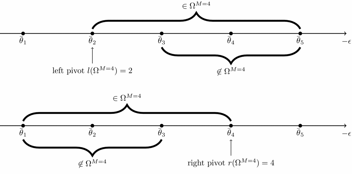
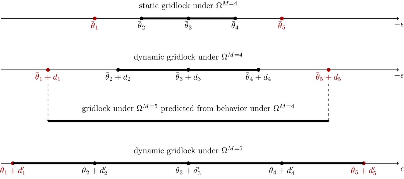
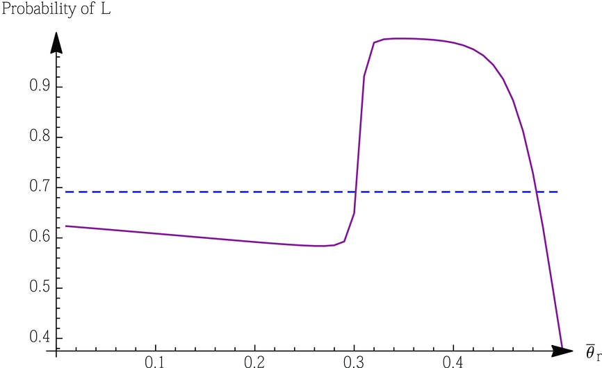
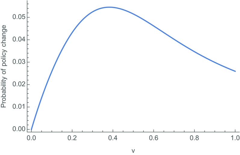



Comments
No Comments have been published for this article.