1 Introduction
The study of double layers in space and atmospheric plasmas had been a trend since the time they were observed to occur naturally in such environments. These double layers can accelerate, decelerate or reflect plasma particles to form a small localized region of a single electric field polarity. Such possibilities had been discussed in connection with auroral kilometric radiation (Alfvén Reference Alfvén1958; Temerin et al.
Reference Temerin, Cerny, Lotko and Mozer1982), the Earth’s bow shock (Bale & Mozer Reference Bale and Mozer2007; Mozer et al.
Reference Mozer, Bale, Bonnell, Chaston, Roth and Wygant2013), the solar wind, solar flares (Jacobsen & Carlqvist Reference Jacobsen and Carlqvist1964), star formation, accretion into neutron stars and double radio galaxies, quasars and extragalactic jets. It had been proposed that small amplitude double layers might explain the fine structures of auroral kilometric radiation (Temerin et al.
Reference Temerin, Cerny, Lotko and Mozer1982; Bujarbarua & Nambu Reference Bujarbarua and Nambu1983). Recently, Mozer et al. (Reference Mozer, Bale, Bonnell, Chaston, Roth and Wygant2013) have reported a large number of different nonlinear structures, including double layers travelling at approximately
 $3100~\text{km}~\text{s}^{-1}$
along the magnetic field, on the basis of observations made by the Van Allen Probe spacecraft in the outer radiation belt (Mozer et al.
Reference Mozer, Bale, Bonnell, Chaston, Roth and Wygant2013; Pottelette, Berthomier & Pickett Reference Pottelette, Berthomier and Pickett2014). The waves observed have been assumed to be electron acoustic (EA) in nature and two components of electrons (hot and cold) were traced during the processed time interval.
Besides the outer radiation belt, in fusion devices, the auroral ionosphere and in the atmospheric environment, plasmas consisting of two components of electrons have been encountered. In such situations, the component with lower temperature (thermal velocity) has been treated as a separate species from that with higher temperature (thermal velocity). The plasmas containing two electron components with similar densities but different temperatures can sustain electron acoustic waves, where the cold electron component provides the inertia whereas the hot electron component is responsible for the restoring force. The phase velocity of the waves lies between the thermal velocities of the cold and hot components of the electrons, i.e.
 $v_{T_{ec}}<v_{\text{phase}}<v_{T_{eh}}$
. Yu & Shukla (Reference Yu and Shukla1983) proved theoretically the existence of those waves in an unmagnetized plasma containing two components of electrons (hot and cold) with a sufficiently rarefied cold electron concentration. These electron acoustic waves can be driven unstable by the relative drift velocities of the two components of electrons. Likewise, a current carrying magnetized plasma can also be driven unstable with respect to electron acoustic waves, provided the ion temperature
 $(T_{i})$
is higher than the electron temperature
 $(T_{e})$
and the wave propagates almost perpendicular to the magnetic field with a phase velocity much less than the ion thermal velocity (Lashmore-Da Vies & Martin Reference Lashmore-Da Vies and Martin1973; Mohan & Buti Reference Mohan and Buti1980). Although the condition
 $T_{i}\gg T_{e}$
is restrictive, such types of plasma are encountered in the Earth’s magnetosphere, solar wind, magnetotail (Gurnett, Frank & Lepping Reference Gurnett, Frank and Lepping1976; Frank & Ackerson Reference Frank and Ackerson1979; Buti, Mohan & Shukla Reference Buti, Mohan and Shukla1980), upstream of the bow shock (Marsch Reference Marsch2008), outer radiation belt (Pizzella & Frank Reference Pizzella and Frank1971) and in laboratory (especially in magnetron-type devices) plasmas (Gurnett et al.
Reference Gurnett, Frank and Lepping1976). Their frequency and wavelength lie between ion and electron gyro-frequencies
 $(\unicode[STIX]{x1D6FA}_{i},\unicode[STIX]{x1D714}_{e})$
, and ion and electron gyro-radii
 $(R_{L},r_{L})$
respectively (Buti et al.
Reference Buti, Mohan and Shukla1980). They may undergo damping or growth depending upon their phase velocities. Extensive theoretical (Guha & Dwivedi Reference Guha and Dwivedi1984; Goswami, Kalita & Bujarbarua Reference Goswami, Kalita and Bujarbarua1986; Goswami & Bujarbarua Reference Goswami and Bujarbarua1987; Kamalam, Steffy & Ghosh Reference Kamalam, Steffy and Ghosh2018) works have been performed to study different electron acoustic nonlinear structures in magnetized plasmas. It has to be mentioned that there is no restriction upon the upper limit of the ion to electron temperature ratio. In some of the previous linear (Lashmore-Da Vies & Martin Reference Lashmore-Da Vies and Martin1973) and nonlinear (Buti et al.
Reference Buti, Mohan and Shukla1980) analyses, it has been considered that
 $T_{i}\sim 10~T_{e}$
. Frank & Ackerson (Reference Frank and Ackerson1979) and Buti et al. (Reference Buti, Mohan and Shukla1980) had given the example of an extra-terrestrial ring current where this condition is satisfied. In that region, the electron temperature is of the order of
 $1-4~\text{keV}$
, whereas the proton temperature is 40 keV. However, in most of the cases,
 $(T_{i}/T_{e})\ll (m_{i}/m_{e})$
. The condition
 $T_{i}\gg T_{e}$
is fulfilled mostly in space and astrophysical environments, where superthermal particles are a ubiquitous component. Therefore, the study of linear and nonlinear electron acoustic waves in the presence of superthermal electrons would provide important information about different phenomena occurred in space and atmospheric environments.
Superthermal particles are characterized by the parameter
 $\unicode[STIX]{x1D705}$
, known as the spectral index. Space-based experiments have confirmed the presence of these superthermal particles in the solar corona, solar wind, planetary magnetosphere and magnetotail and the Earth’s ionosphere (Maksimovic, Pierrard & Lemaire Reference Maksimovic, Pierrard and Lemaire1997; Pierrard & Lazar Reference Pierrard and Lazar2010; Dutta & Goswami Reference Dutta and Goswami2019). These particles have been characterized by wave–particle interactions rather than by binary collisions. Therefore, they cannot relax to thermal equilibrium and their trajectories cannot be studied with the help of the Maxwell–Boltzmann distribution. It has been observed that the generalized Lorentzian, or kappa, distribution is convenient to describe the velocity distribution of these particles which is expressed as (Vasyliunas Reference Vasyliunas1968),
 $$\begin{eqnarray}\displaystyle f_{s}^{\unicode[STIX]{x1D705}}(v_{s})=\frac{n_{s0}}{(\unicode[STIX]{x03C0}\unicode[STIX]{x1D705}\unicode[STIX]{x1D703}_{s}^{2})^{3/2}}\frac{\unicode[STIX]{x1D6E4}(\unicode[STIX]{x1D705}+1)}{\unicode[STIX]{x1D6E4}(\unicode[STIX]{x1D705}-1/2)}\left(1+\frac{v_{s}^{2}}{\unicode[STIX]{x1D705}\unicode[STIX]{x1D703}_{s}^{2}}\right)^{-(\unicode[STIX]{x1D705}+1)}. & & \displaystyle\end{eqnarray}$$
Here, the spectral index represents the degree of superthermality. It can have values within
 $[1.5,\infty )$
. The significance of this distribution function is that in the limit
 $\unicode[STIX]{x1D705}\rightarrow \infty$
, the distribution converges to the Maxwell–Boltzmann distribution. Small value of
 $\unicode[STIX]{x1D705}$
indicates a population of highly superthermal particles:
 $\unicode[STIX]{x1D703}_{s}$
is the effective thermal velocity of the plasma species
 $s$
, and is related to the usual thermal velocity
 $v_{T_{s}}\,(=\sqrt[]{T_{s}/m_{s}})$
by
 $\unicode[STIX]{x1D703}_{s}^{2}=(1-3/2\unicode[STIX]{x1D705})v_{T_{s}}^{2}$
;
 $m_{s}$
and
 $v_{s}$
are the mass and velocity of the particles with characteristic kinetic temperature
 $T_{s}$
(the temperature of the equivalent Maxwellian with the same average kinetic energy);
 $n_{s0}$
is their equilibrium number density, and
 $\unicode[STIX]{x1D6E4}(x)$
is the gamma function. The suffix
 $s$
is used to describe a particular plasma species.
In the present work, the plasma model is composed of superthermal electrons and ions along with a fraction of cold fluid electrons. The existence of small amplitude electron acoustic double layers has been studied using the Sagdeev pseudo-potential method for the small amplitude regime. The cold component of electrons is assumed to be inertial with temperature
 $(T_{ec})$
much lower than that of the superthermal ions
 $(T_{i})$
and electrons
 $(T_{eh})$
. The effect of the hot component of electrons on the nature of the electron acoustic double layers is also studied. Such a type of plasma is generally available in most of space and atmospheric environments, especially in the outer radiation belt. Although the Earth’s outer radiation belt is mainly dominated by highly energetic electrons
 $(0.1-10~\text{MeV})$
trapped by the Earth’s magnetosphere, they are removed constantly by collisions with the Earth’s atmosphere and losses to the magnetopause. The remaining part of the electrons (also termed seed electrons) are observed to be of
 ${\sim}1-100~\text{keV}$
(Temerin et al.
Reference Temerin, Cerny, Lotko and Mozer1982; Mozer et al.
Reference Mozer, Bale, Bonnell, Chaston, Roth and Wygant2013; Agapitov et al.
Reference Agapitov, Krasnoselskikh, Mozer, Artemyeva and Volokitin2015). On the other hand, the observation of charged particle distributions in the Earth’s radiation belt proved the existence of large intensities of protons within the energy range
 $200~\text{eV}\lesssim T_{i}\lesssim 1~\text{MeV}$
(Pizzella & Frank Reference Pizzella and Frank1971). Recently, Fernandes et al. (Reference Fernandes, Larsen, Thomsen, Skoug, Reeves, Denton, Friedel, Funsten, Goldstein and Henderson2017) reported the existence of 10 keV
 $\text{O}^{+}$
, and
 $\text{He}^{+}$
in the radiation belt by using the data obtained from the HOPE (helium–oxygen–proton–electron) mass spectrometer of the Van Allen Probes. In addition, from the observation and satellite data in the radiation belt, electron and ion populations following a kappa distribution with
 $2<\unicode[STIX]{x1D705}<6$
have been detected (Pierrard & Lazar Reference Pierrard and Lazar2010). Therefore we have assumed that our proposed plasma model will be suitable for the outer radiation belt and the results obtained from this study will be helpful to understand the dynamics of plasma waves in such environments. Interestingly, the proposed plasma model generates potential drops and propagation speeds almost equal to those reported by Mozer et al. (Reference Mozer, Bale, Bonnell, Chaston, Roth and Wygant2013).
The manuscript is arranged as follows; in the next section (§ 2), the theoretical model including the linear (§ 2.1) and nonlinear analyses (§ 2.2) is presented. The results are discussed in § 3 including the linear analysis of the electron acoustic wave (§ 3.1), the determination of the existence domain (§ 3.2), the generation of the electron acoustic double layer (§ 3.3), the effect of different superthermal parameters on the double layer (§ 3.4) and a table showing the variation of the amplitude and the speed of the nonlinear structure with different plasma parameters (§ 3.5). The manuscript is concluded with a brief conclusion in § 4.
2 Theoretical model
2.1 The linear analysis
The modelled plasma consists of a single component of singly ionized
 $(Z=1)$
ions and two components of electrons of distinct temperature. To distinguish the electron components, they are termed as hot and cold components depending upon their temperature. The density and temperature of the ions and hot electrons are assumed to be
 $n_{i}=n_{0}\sim 1~\text{cm}^{-3}$
,
 $T_{i}\sim 10~\text{keV}-1~\text{MeV}$
, and
 $T_{eh}=10~\text{keV}$
. The cold electron density is below a few tenths of the total electron density (
 $n_{0}$
) (Pizzella & Frank Reference Pizzella and Frank1971; Mozer et al.
Reference Mozer, Bale, Bonnell, Chaston, Roth and Wygant2013; Fernandes et al.
Reference Fernandes, Larsen, Thomsen, Skoug, Reeves, Denton, Friedel, Funsten, Goldstein and Henderson2017; Dillard et al.
Reference Dillard, Vasko, Mozer, Agapitov and Bonnell2018). The uniform magnetic field is along the
 $z$
-direction i.e.
 $\boldsymbol{B}_{\mathbf{0}}=B_{0}\hat{z}$
. The electron acoustic wave is assumed to propagate in the
 $x{-}z$
plane along a fixed direction, making an angle
 $\unicode[STIX]{x1D703}$
with the magnetic field such that,
 $0<\cos \unicode[STIX]{x1D703}\ll (m_{e}/m_{i})^{1/2}$
. For a wave propagating nearly across the magnetic field, the thermal velocity of the cold component of electrons is smaller than the phase velocity of the wave along the magnetic field. Thus, for such a situation,
 $v_{T_{ec}}<C_{e}$
, whereas
 $C_{e}\cos \unicode[STIX]{x1D703}\ll v_{T_{i}}<v_{T_{eh}}$
. Here,
 $C_{e}=\sqrt[]{T_{i}/m_{e}}$
, and
 $C_{e}\cos \unicode[STIX]{x1D703}$
is the phase velocity of the electron acoustic wave. The electron inertia is important for the dynamics of such waves. Therefore, the motion of the cold component of electrons is described with the fluid equations,
 $$\begin{eqnarray}\displaystyle & \displaystyle \frac{\unicode[STIX]{x2202}n_{ec}}{\unicode[STIX]{x2202}t}+\unicode[STIX]{x1D735}\boldsymbol{\cdot }(n_{ec}v)=0, & \displaystyle\end{eqnarray}$$
 $$\begin{eqnarray}\displaystyle & \displaystyle m_{e}\frac{\unicode[STIX]{x2202}v}{\unicode[STIX]{x2202}t}+\boldsymbol{v}\boldsymbol{\cdot }\unicode[STIX]{x1D735}\boldsymbol{v}=-e(\boldsymbol{E}+\boldsymbol{v}\times \boldsymbol{B}_{\mathbf{0}}). & \displaystyle\end{eqnarray}$$
Equations (2.1) and (2.2) are the continuity and momentum equation, respectively. Here,
 $n_{ec}$
, is the number density of the cold electron component whereas
 $\boldsymbol{v}(=v_{x}\boldsymbol{i}+v_{y}\boldsymbol{j}+v_{z}\boldsymbol{k})$
is their velocity vector;
 $\boldsymbol{E}$
is the electric field. As the thermal velocities of the hot component of the electrons and the ions are greater than the phase velocity of the wave propagating along the magnetic field, they can be considered as inertialess. So, the hot component of electrons and the ions are assumed to be superthermal and their respective number densities are expressed as,
 $$\begin{eqnarray}\displaystyle & \displaystyle n_{eh}=n_{h0}\left(1-\frac{e\unicode[STIX]{x1D719}}{(\unicode[STIX]{x1D705}_{e}-3/2)T_{eh}}\right)^{-\unicode[STIX]{x1D705}_{e}+1/2}, & \displaystyle\end{eqnarray}$$
 $$\begin{eqnarray}\displaystyle & \displaystyle n_{i}=n_{i0}\left(1+\frac{e\unicode[STIX]{x1D719}}{(\unicode[STIX]{x1D705}_{i}-3/2)T_{i}}\right)^{-\unicode[STIX]{x1D705}_{i}+1/2}. & \displaystyle\end{eqnarray}$$
Here, we have considered that the electron Debye length is smaller than the electron gyro-radius. Therefore, the whole set of equations is closed with the quasi-neutrality condition (Goswami & Bujarbarua Reference Goswami and Bujarbarua1987). The quasi-neutrality condition states,
 $$\begin{eqnarray}\displaystyle n_{i}=n_{ec}+n_{eh}. & & \displaystyle\end{eqnarray}$$
In (2.3) and (2.4)
 $n_{eh}$
and
 $n_{i}$
represent the number densities of hot electron component and the ions with respective equilibrium values
 $n_{h0}$
and
 $n_{i0}$
. The electrostatic potential is represented by
 $\unicode[STIX]{x1D719}$
;
 $\unicode[STIX]{x1D705}_{e}$
and
 $\unicode[STIX]{x1D705}_{i}$
are the superthermal indices of the hot component of electrons and the ions. The number densities have been derived by integrating the generalized Lorentzian (or kappa) distribution function given in (1.1).
Linearizing equations (2.1)–(2.5) the linear dispersion relation has been derived and is,
 $$\begin{eqnarray}\displaystyle \unicode[STIX]{x1D714}^{4}-\unicode[STIX]{x1D714}^{2}(\unicode[STIX]{x1D714}_{e}^{2}+k^{2}C_{e}^{2}a)+k^{2}C_{e}^{2}a\unicode[STIX]{x1D714}_{e}^{2}\cos ^{2}\unicode[STIX]{x1D703}=0. & & \displaystyle\end{eqnarray}$$
Here,
 $\unicode[STIX]{x1D714}$
and
 $k$
are the angular frequency and wavenumber of the electron acoustic wave, respectively:
 $\unicode[STIX]{x1D714}_{e}(=eB_{0}/m_{e})$
is the electron gyro-frequency and
 $C_{e}=(\sqrt[]{T_{i}/m_{e}})$
is the electron acoustic velocity;
 $a$
is a constant and is expressed as
 $a=[\unicode[STIX]{x1D6FC}(\unicode[STIX]{x1D705}_{e}-1/2)/\unicode[STIX]{x1D70E}_{h}(\unicode[STIX]{x1D705}_{e}-3/2)+(1+\unicode[STIX]{x1D6FC})(\unicode[STIX]{x1D705}_{i}-1/2)/(\unicode[STIX]{x1D705}_{i}-3/2)]^{-1}$
;
 $\unicode[STIX]{x1D70E}_{h}$
is the hot electron to ion temperature ratio
 $(T_{eh}/T_{i})$
. If
 $n_{s0}~(s=i,c,h)$
indicates the number densities of the ions, cold electrons and hot electrons, respectively at equilibrium, then
 $\unicode[STIX]{x1D6FC}=n_{h0}/n_{c0}$
and
 $(1+\unicode[STIX]{x1D6FC})=n_{i0}/n_{c0}$
are the density ratios. Equation (2.6) is a quadratic in
 $\unicode[STIX]{x1D714}^{2}$
and solving the equation we get,
 $$\begin{eqnarray}\displaystyle \unicode[STIX]{x1D714}_{\pm }^{2}={\textstyle \frac{1}{2}}[\unicode[STIX]{x1D714}_{e}^{2}+k^{2}C_{e}^{2}a\pm \sqrt[]{(\unicode[STIX]{x1D714}_{e}^{2}+k^{2}C_{e}^{2}a)^{2}-4k^{2}C_{e}^{2}a\unicode[STIX]{x1D714}_{e}^{2}\cos ^{2}\unicode[STIX]{x1D703}}]. & & \displaystyle\end{eqnarray}$$
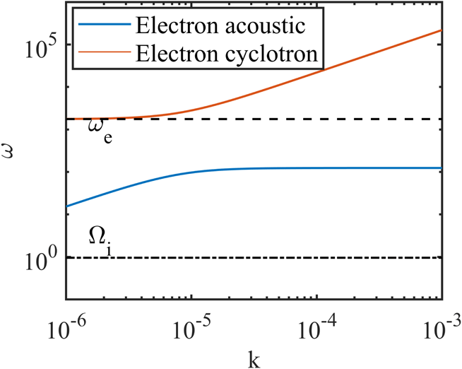
To study different modes, the dispersion relation expressed in (2.7) is plotted in figure 1. From the figure, the presence of the electron acoustic wave in the modelled plasma can be well explained.
Dispersion of the plasma wave for different branches of angular frequency (
 $\unicode[STIX]{x1D714}_{-}$
or electron acoustic: blue line and
 $\unicode[STIX]{x1D714}_{+}$
or electron cyclotron: red line). The compositional parameters assumed here are,
 $l_{z}=0.005,\unicode[STIX]{x1D6FC}=0.1,\unicode[STIX]{x1D705}_{i}=2.0,\unicode[STIX]{x1D705}_{e}=1.6$
,
 $\unicode[STIX]{x1D70E}_{h}=0.2$
and
 $B_{0}=10~\text{nT}$
.

2.2 The nonlinear analysis
To perform the nonlinear analysis, equations (2.1)–(2.4) have been normalized with appropriate normalization parameters as given below,
 $$\begin{eqnarray}\displaystyle N_{s}=n_{s}/(n_{s0}),\quad U_{r}=v_{r}/(C_{e}\cos \unicode[STIX]{x1D703}),\quad \unicode[STIX]{x1D6F7}=e\unicode[STIX]{x1D719}/T_{i},\quad \unicode[STIX]{x1D709}_{r}=r/r_{L},\quad \unicode[STIX]{x1D70F}=t/(\unicode[STIX]{x1D714}_{e}\cos \unicode[STIX]{x1D703})^{-1}. & & \displaystyle \nonumber\\ \displaystyle & & \displaystyle\end{eqnarray}$$
Here,
 $N_{s}$
and
 $n_{s}$
represent the normalized and un-normalized number densities of cold electrons
 $(N_{ec},n_{ec})$
, hot electrons
 $(N_{eh},n_{eh})$
and ions
 $(N_{i},n_{i})$
respectively. On the other hand,
 $U_{r}$
and
 $v_{r}$
represents the normalized and un-normalized velocities of the cold electron component along the
 $x,y$
and
 $z$
directions:
 $r$
represents
 $x,y$
and
 $z$
, and thus
 $\unicode[STIX]{x1D709}_{r}$
represents
 $\unicode[STIX]{x1D709}_{x},\unicode[STIX]{x1D709}_{y}$
, and
 $\unicode[STIX]{x1D709}_{z}$
respectively;
 $r_{L}=V_{T_{ec}}/\unicode[STIX]{x1D714}_{e}$
is the electron gyro-radius. Here,
 $V_{T_{ec}}=\sqrt[]{T_{ec}/m_{e}}$
is the thermal velocity of the cold electron component. Finally, the normalized set of equations take the form,
 $$\begin{eqnarray}\displaystyle & \displaystyle \frac{\unicode[STIX]{x2202}N_{ec}}{\unicode[STIX]{x2202}\unicode[STIX]{x1D70F}}+\frac{\unicode[STIX]{x2202}}{\unicode[STIX]{x2202}\unicode[STIX]{x1D709}_{x}}(N_{ec}U_{x})+\frac{\unicode[STIX]{x2202}}{\unicode[STIX]{x2202}\unicode[STIX]{x1D709}_{z}}(N_{ec}U_{z})=0, & \displaystyle\end{eqnarray}$$
 $$\begin{eqnarray}\displaystyle & \displaystyle \frac{\unicode[STIX]{x2202}U_{x}}{\unicode[STIX]{x2202}\unicode[STIX]{x1D70F}}+\left(U_{x}\frac{\unicode[STIX]{x2202}U_{x}}{\unicode[STIX]{x2202}\unicode[STIX]{x1D709}_{x}}+U_{z}\frac{\unicode[STIX]{x2202}U_{x}}{\unicode[STIX]{x2202}\unicode[STIX]{x1D709}_{z}}\right)=\frac{1}{\cos ^{2}\unicode[STIX]{x1D703}}\frac{\unicode[STIX]{x2202}\unicode[STIX]{x1D6F7}}{\unicode[STIX]{x2202}\unicode[STIX]{x1D709}_{x}}-\frac{1}{\cos \unicode[STIX]{x1D703}}U_{y}, & \displaystyle\end{eqnarray}$$
 $$\begin{eqnarray}\displaystyle & \displaystyle \frac{\unicode[STIX]{x2202}U_{y}}{\unicode[STIX]{x2202}\unicode[STIX]{x1D70F}}+\left(U_{x}\frac{\unicode[STIX]{x2202}U_{y}}{\unicode[STIX]{x2202}\unicode[STIX]{x1D709}_{x}}+U_{z}\frac{\unicode[STIX]{x2202}U_{y}}{\unicode[STIX]{x2202}\unicode[STIX]{x1D709}_{z}}\right)=\frac{1}{\cos \unicode[STIX]{x1D703}}U_{x}, & \displaystyle\end{eqnarray}$$
 $$\begin{eqnarray}\displaystyle & \displaystyle \frac{\unicode[STIX]{x2202}U_{z}}{\unicode[STIX]{x2202}\unicode[STIX]{x1D70F}}+\left(U_{x}\frac{\unicode[STIX]{x2202}U_{z}}{\unicode[STIX]{x2202}\unicode[STIX]{x1D709}_{x}}+U_{z}\frac{\unicode[STIX]{x2202}U_{z}}{\unicode[STIX]{x2202}\unicode[STIX]{x1D709}_{z}}\right)=\frac{1}{\cos ^{2}\unicode[STIX]{x1D703}}\frac{\unicode[STIX]{x2202}\unicode[STIX]{x1D6F7}}{\unicode[STIX]{x2202}\unicode[STIX]{x1D709}_{z}}. & \displaystyle\end{eqnarray}$$
 $$\begin{eqnarray}\displaystyle & \displaystyle N_{eh}=\left(1-\frac{\unicode[STIX]{x1D6F7}}{\unicode[STIX]{x1D70E}_{h}\left(\unicode[STIX]{x1D705}_{e}-{\displaystyle \frac{3}{2}}\right)}\right)^{-\unicode[STIX]{x1D705}_{e}+1/2}, & \displaystyle\end{eqnarray}$$
 $$\begin{eqnarray}\displaystyle & \displaystyle N_{i}=\left(1+\frac{\unicode[STIX]{x1D6F7}}{\left(\unicode[STIX]{x1D705}_{i}-{\displaystyle \frac{3}{2}}\right)}\right)^{-\unicode[STIX]{x1D705}_{i}+1/2}. & \displaystyle\end{eqnarray}$$
To explore the nature of the double layers that may be generated in such environments, the Sagdeev pseudo-potential method for the small amplitude regime
 $(\unicode[STIX]{x1D6F7}\ll 1)$
has been followed. To proceed, a comoving frame having coordinate
 $\unicode[STIX]{x1D702}=l_{x}\unicode[STIX]{x1D709}_{x}+l_{z}\unicode[STIX]{x1D709}_{z}-M\unicode[STIX]{x1D70F}$
has been considered. Here
 $M$
is the Mach number, the normalized velocity of the comoving frame or the nonlinear structures generated in the plasma:
 $l_{x}$
and
 $l_{z}$
are the direction cosines with
 $l_{x}=k_{x}/k=\text{sin}\,\unicode[STIX]{x1D703}$
and
 $l_{z}=k_{z}/k=\cos \unicode[STIX]{x1D703}$
such that,
 $l_{x}^{2}+l_{z}^{2}=1$
;
 $\boldsymbol{k}$
is the wave vector having components
 $k_{x}$
, and
 $k_{z}$
in the
 $x$
-, and
 $z$
-directions. Now, transforming the coordinates to the new one
 $(\unicode[STIX]{x1D702})$
and simplifying (2.9)–(2.12) using the boundary conditions (B.C.s):
 $N_{ec}\rightarrow 1$
and
 $\unicode[STIX]{x1D6F7},U_{x},U_{y},U_{z}\rightarrow 0$
at
 $\unicode[STIX]{x1D702}\rightarrow \pm \infty$
, finally a new set of equations is derived and is,
 $$\begin{eqnarray}\displaystyle & \displaystyle l_{x}U_{x}+l_{z}U_{z}=M\left(1-\frac{1}{N_{ec}}\right), & \displaystyle\end{eqnarray}$$
 $$\begin{eqnarray}\displaystyle & \displaystyle -\frac{M}{N_{ec}}\frac{\unicode[STIX]{x2202}U_{x}}{\unicode[STIX]{x2202}\unicode[STIX]{x1D702}}=\frac{l_{x}}{l_{z}^{2}}\frac{\unicode[STIX]{x2202}\unicode[STIX]{x1D6F7}}{\unicode[STIX]{x2202}\unicode[STIX]{x1D702}}-\frac{1}{l_{z}}U_{y}, & \displaystyle\end{eqnarray}$$
 $$\begin{eqnarray}\displaystyle & \displaystyle -\frac{M}{N_{ec}}\frac{\unicode[STIX]{x2202}U_{y}}{\unicode[STIX]{x2202}\unicode[STIX]{x1D702}}=\frac{1}{l_{z}}U_{x}, & \displaystyle\end{eqnarray}$$
 $$\begin{eqnarray}\displaystyle & \displaystyle -\frac{M}{N_{ec}}\frac{\unicode[STIX]{x2202}U_{z}}{\unicode[STIX]{x2202}\unicode[STIX]{x1D702}}=\frac{1}{l_{z}}\frac{\unicode[STIX]{x2202}\unicode[STIX]{x1D6F7}}{\unicode[STIX]{x2202}\unicode[STIX]{x1D702}}. & \displaystyle\end{eqnarray}$$
Now, integrating equation (2.18),
 $$\begin{eqnarray}\displaystyle U_{z}=-\frac{1}{Ml_{z}}I(\unicode[STIX]{x1D6F7}). & & \displaystyle\end{eqnarray}$$
Here,
 $I(\unicode[STIX]{x1D6F7})=\int N_{ec}\,\text{d}\unicode[STIX]{x1D6F7}$
. Using (2.15) and (2.19) in (2.16), the expression for
 $U_{y}$
is derived,
 $$\begin{eqnarray}\displaystyle U_{y}=\frac{1}{l_{x}l_{z}}\left[1+\frac{M^{2}l_{z}^{2}}{N_{ec}^{3}}\frac{\unicode[STIX]{x2202}N_{ec}}{\unicode[STIX]{x2202}\unicode[STIX]{x1D6F7}}\right]\frac{\unicode[STIX]{x2202}\unicode[STIX]{x1D6F7}}{\unicode[STIX]{x2202}\unicode[STIX]{x1D702}}. & & \displaystyle\end{eqnarray}$$
Now, substituting the expressions of (2.15), (2.19) and (2.20) in (2.17), finally an equation is derived which contains information from all of the dynamical equations,
 $$\begin{eqnarray}\displaystyle -\frac{\unicode[STIX]{x2202}}{\unicode[STIX]{x2202}\unicode[STIX]{x1D702}}\left[A\frac{\unicode[STIX]{x2202}\unicode[STIX]{x1D6F7}}{\unicode[STIX]{x2202}\unicode[STIX]{x1D702}}\right]=\left[N_{ec}-1+\frac{N_{ec}}{M^{2}}I(\unicode[STIX]{x1D6F7})\right]. & & \displaystyle\end{eqnarray}$$
Here,
 $A=[1+(M^{2}l_{z}^{2}/N_{ec}^{3})(\unicode[STIX]{x2202}N_{ec}/\unicode[STIX]{x2202}\unicode[STIX]{x1D6F7})]\approx 1-M^{2}l_{z}^{2}\unicode[STIX]{x1D70C}_{1}$
(the expression for
 $\unicode[STIX]{x1D70C}_{1}$
is expressed later in (2.25a
)). For any value of the parameters
 $\unicode[STIX]{x1D6FC},\unicode[STIX]{x1D705}_{i},\unicode[STIX]{x1D705}_{e}$
and
 $\unicode[STIX]{x1D70E}_{h}$
, it is observed that
 $A\approx 1$
for
 $0<\cos \unicode[STIX]{x1D703}\ll (m_{e}/m_{i})^{1/2}$
. On further simplification, equation (2.21) yields,
 $$\begin{eqnarray}\displaystyle \frac{1}{2}\frac{\unicode[STIX]{x2202}}{\unicode[STIX]{x2202}\unicode[STIX]{x1D6F7}}\left(A\frac{\unicode[STIX]{x2202}\unicode[STIX]{x1D6F7}}{\unicode[STIX]{x2202}\unicode[STIX]{x1D702}}\right)^{2}=A\left[1-N_{ec}-\frac{N_{ec}}{M^{2}}I(\unicode[STIX]{x1D6F7})\right]. & & \displaystyle\end{eqnarray}$$
Now, the normalized quasi-neutrality condition states,
 $$\begin{eqnarray}\displaystyle N_{ec}=(1+\unicode[STIX]{x1D6FC})N_{i}-\unicode[STIX]{x1D6FC}N_{eh}. & & \displaystyle\end{eqnarray}$$
Expanding the densities of superthermal ions and electrons about their equilibrium densities and rearranging the terms in ascending order of the power of
 $\unicode[STIX]{x1D6F7}$
, finally the equation (2.23) becomes,
 $$\begin{eqnarray}\displaystyle N_{ec}=1-\unicode[STIX]{x1D70C}_{1}\unicode[STIX]{x1D6F7}+\unicode[STIX]{x1D70C}_{2}\unicode[STIX]{x1D6F7}^{2}-\unicode[STIX]{x1D70C}_{3}\unicode[STIX]{x1D6F7}^{3}. & & \displaystyle\end{eqnarray}$$
Where,
 $$\begin{eqnarray}\displaystyle & \displaystyle \unicode[STIX]{x1D70C}_{1}=\frac{(1+\unicode[STIX]{x1D6FC})(2\unicode[STIX]{x1D705}_{i}-1)}{(2\unicode[STIX]{x1D705}_{i}-3)}+\frac{\unicode[STIX]{x1D6FC}(2\unicode[STIX]{x1D705}_{e}-1)}{\unicode[STIX]{x1D70E}_{h}(2\unicode[STIX]{x1D705}_{e}-3)}, & \displaystyle\end{eqnarray}$$
 $$\begin{eqnarray}\displaystyle & \displaystyle \unicode[STIX]{x1D70C}_{2}=\frac{(1+\unicode[STIX]{x1D6FC})(4\unicode[STIX]{x1D705}_{i}^{2}-1)}{2(2\unicode[STIX]{x1D705}_{i}-3)^{2}}-\frac{\unicode[STIX]{x1D6FC}(4\unicode[STIX]{x1D705}_{e}^{2}-1)}{2\unicode[STIX]{x1D70E}_{h}^{2}(2\unicode[STIX]{x1D705}_{e}-3)^{2}}, & \displaystyle\end{eqnarray}$$
 $$\begin{eqnarray}\displaystyle & \displaystyle \unicode[STIX]{x1D70C}_{3}=\frac{(1+\unicode[STIX]{x1D6FC})(4\unicode[STIX]{x1D705}_{i}^{2}-1)(2\unicode[STIX]{x1D705}_{i}+3)}{6(2\unicode[STIX]{x1D705}_{i}-3)^{3}}+\frac{\unicode[STIX]{x1D6FC}(4\unicode[STIX]{x1D705}_{e}^{2}-1)(2\unicode[STIX]{x1D705}_{e}+3)}{6\unicode[STIX]{x1D70E}_{h}^{3}(2\unicode[STIX]{x1D705}_{e}-3)^{3}}. & \displaystyle\end{eqnarray}$$
 $N_{ec}$
in (2.22) and simplifying we get,
 $$\begin{eqnarray}\displaystyle \frac{1}{2}\frac{\unicode[STIX]{x2202}}{\unicode[STIX]{x2202}\unicode[STIX]{x1D6F7}}\left(A\frac{\unicode[STIX]{x2202}\unicode[STIX]{x1D6F7}}{\unicode[STIX]{x2202}\unicode[STIX]{x1D702}}\right)^{2}=A[B_{1}\unicode[STIX]{x1D6F7}-B_{2}\unicode[STIX]{x1D6F7}^{2}+B_{3}\unicode[STIX]{x1D6F7}^{3}]. & & \displaystyle\end{eqnarray}$$
Here,
 $$\begin{eqnarray}\displaystyle B_{1} & = & \displaystyle \frac{(1+\unicode[STIX]{x1D6FC})(2\unicode[STIX]{x1D705}_{i}-1)}{(2\unicode[STIX]{x1D705}_{i}-3)}+\frac{\unicode[STIX]{x1D6FC}(2\unicode[STIX]{x1D705}_{e}-1)}{\unicode[STIX]{x1D70E}_{h}(2\unicode[STIX]{x1D705}_{e}-3)}-\frac{1}{M^{2}},\end{eqnarray}$$
 $$\begin{eqnarray}\displaystyle B_{2} & = & \displaystyle \frac{(1+\unicode[STIX]{x1D6FC})(4\unicode[STIX]{x1D705}_{i}^{2}-1)}{2(\unicode[STIX]{x1D705}_{i}-3)^{2}}-\frac{\unicode[STIX]{x1D6FC}(4\unicode[STIX]{x1D705}_{e}^{2}-1)}{2\unicode[STIX]{x1D70E}_{h}^{2}(2\unicode[STIX]{x1D705}_{e}-3)^{2}}\nonumber\\ \displaystyle & & \displaystyle -\,\frac{3}{2M^{2}}\left[\frac{(1+\unicode[STIX]{x1D6FC})(2\unicode[STIX]{x1D705}_{i}-1)}{(2\unicode[STIX]{x1D705}_{i}-3)}+\frac{\unicode[STIX]{x1D6FC}(2\unicode[STIX]{x1D705}_{e}-1)}{\unicode[STIX]{x1D70E}_{h}(2\unicode[STIX]{x1D705}_{e}-3)}\right],\end{eqnarray}$$
and
 $$\begin{eqnarray}\displaystyle B_{3} & = & \displaystyle \frac{(1+\unicode[STIX]{x1D6FC})(4\unicode[STIX]{x1D705}_{i}^{2}-1)(2\unicode[STIX]{x1D705}_{i}+3)}{6(\unicode[STIX]{x1D705}_{i}-3)^{3}}+\frac{\unicode[STIX]{x1D6FC}(4\unicode[STIX]{x1D705}_{e}^{2}-1)(2\unicode[STIX]{x1D705}_{e}+3)}{6\unicode[STIX]{x1D70E}_{h}^{3}(2\unicode[STIX]{x1D705}_{e}-3)^{3}}\nonumber\\ \displaystyle & & \displaystyle -\,\frac{4}{3M^{2}}\left[\frac{(1+\unicode[STIX]{x1D6FC})(4\unicode[STIX]{x1D705}_{i}^{2}-1)}{2(2\unicode[STIX]{x1D705}_{i}-3)^{2}}-\frac{\unicode[STIX]{x1D6FC}(4\unicode[STIX]{x1D705}_{e}^{2}-1)}{2\unicode[STIX]{x1D70E}_{h}^{2}(2\unicode[STIX]{x1D705}_{e}-3)^{2}}\right]\nonumber\\ \displaystyle & & \displaystyle -\,\frac{1}{2M^{2}}\left[\frac{(1+\unicode[STIX]{x1D6FC})(2\unicode[STIX]{x1D705}_{i}-1)}{(2k_{i}-3)}+\frac{\unicode[STIX]{x1D6FC}(2\unicode[STIX]{x1D705}_{e}-1)}{\unicode[STIX]{x1D70E}_{h}(2\unicode[STIX]{x1D705}_{e}-3)}\right]^{2}.\end{eqnarray}$$
Integrating equation (2.26) finally, it can be written in the energy integral form and is (Goswami et al. Reference Goswami, Kalita and Bujarbarua1986),
 $$\begin{eqnarray}\displaystyle \frac{1}{2}\left(A\frac{\unicode[STIX]{x2202}\unicode[STIX]{x1D6F7}}{\unicode[STIX]{x2202}\unicode[STIX]{x1D702}}\right)^{2}+V(\unicode[STIX]{x1D6F7})=0. & & \displaystyle\end{eqnarray}$$
In (2.28),
 $V(\unicode[STIX]{x1D6F7})$
is the pseudo-potential, better known as the Sagdeev potential, of the plasma system with
 $\unicode[STIX]{x1D6F7}$
as the ‘spatial coordinate’ (pseudo-position) and
 $\unicode[STIX]{x1D702}$
as the ‘time’ and is expressed as,
 $$\begin{eqnarray}\displaystyle V(\unicode[STIX]{x1D6F7})=-{\textstyle \frac{1}{2}}B_{1}\unicode[STIX]{x1D6F7}^{2}+{\textstyle \frac{1}{3}}B_{2}\unicode[STIX]{x1D6F7}^{3}-{\textstyle \frac{1}{4}}B_{3}\unicode[STIX]{x1D6F7}^{4}. & & \displaystyle\end{eqnarray}$$
Thus, equation (2.26) implies
 $(1/2)~\unicode[STIX]{x2202}/\unicode[STIX]{x2202}\unicode[STIX]{x1D6F7}(A\unicode[STIX]{x2202}\unicode[STIX]{x1D6F7}/\unicode[STIX]{x2202}\unicode[STIX]{x1D702})^{2}-V^{^{\prime }}(\unicode[STIX]{x1D6F7})=0$
, where the prime denotes the derivative with respect to
 $\unicode[STIX]{x1D6F7}$
. On solving (2.26) and (2.28) by applying the conditions for double layers i.e. at
 $\unicode[STIX]{x1D6F7}=0,\pm \unicode[STIX]{x1D713},V(\unicode[STIX]{x1D6F7})=0$
(electric field vanishes at the boundary), and
 $V^{^{\prime }}(\unicode[STIX]{x1D6F7})=0$
(quasi-neutrality holds at the boundary), the potential of the double layers has been finally derived and is,
 $$\begin{eqnarray}\displaystyle \unicode[STIX]{x1D6F7}=\frac{\unicode[STIX]{x1D713}}{2}\left(1+\tanh \sqrt[]{\frac{B_{3}}{8A}}\unicode[STIX]{x1D713}\unicode[STIX]{x1D702}\right). & & \displaystyle\end{eqnarray}$$
Here,
 $\unicode[STIX]{x1D713}(=2B_{2}/3B_{3})$
is the amplitude and
 $\sqrt[]{8A/B_{3}}$
is the width of the double layers. Already from the expression of
 $A$
, it has been observed that
 $A\approx 1$
. Hence, for the generation of the double layers
 $B_{3}$
must be greater than
 $0$
. The nature and size of the double layers generated in such an environment can be discussed with the help of (2.30), and this is done in the next section (§§ 3.3–3.4).
3 Results and discussions
3.1 The linear wave analysis
In this analytical study, a magnetized plasma consisting of a single species of superthermal ions, along with two species of electrons, has been considered. On performing the linear analysis of the governing equations, the dispersion relation has been derived and is expressed in (2.6). On further simplification it leads to (2.7). The dispersion relation for such plasma waves has been expressed in (2.6) which on further simplification has led to (2.7). The equation (2.7) consists of two branches of
 $\unicode[STIX]{x1D714}$
, viz. the ‘+’ branch
 $(\unicode[STIX]{x1D714}_{+})$
, and the ‘
 $-$
’ branch
 $(\unicode[STIX]{x1D714}_{-})$
. The dispersion relations for the two branches are depicted in figure 1. From the figure, it has been observed that for
 $\unicode[STIX]{x1D714}\geqslant \unicode[STIX]{x1D714}_{e}$
, the plasma can sustain an electron cyclotron-like wave, whereas, for
 $\unicode[STIX]{x1D6FA}_{i}\ll \unicode[STIX]{x1D714}\ll \unicode[STIX]{x1D714}_{e}$
, the plasma can sustain an electron acoustic wave. It has been mentioned earlier that the electron acoustic wave has a frequency within the electron and ion gyro-frequencies, which is clearly observable from the figure.
3.2 The existence domain
After linear analysis of the waves, the existence domains for the double layers are studied. It is clear from (2.29) that at the origin
 $(\unicode[STIX]{x1D6F7}=0)$
,
 $V(\unicode[STIX]{x1D6F7})$
has a double root for the undisturbed conditions, since
 $V^{^{\prime }}(\unicode[STIX]{x1D6F7})$
also vanishes there. However, in order to get solitary wave solutions, one need to encounter root(s) of
 $V(\unicode[STIX]{x1D6F7})$
at
 $|\unicode[STIX]{x1D6F7}|>0$
also. Single roots of
 $V(\unicode[STIX]{x1D6F7})$
give rise to hill- (positive) or dip- (negative) like solitons. Double roots of
 $V(\unicode[STIX]{x1D6F7})$
give potential kinks (double layers) where
 $\unicode[STIX]{x1D6F7}$
changes from one value at
 $-\infty$
to another value at
 $+\infty$
. Further, the solitary structure (soliton and DL) solutions demand that
 $V^{^{\prime \prime }}(\unicode[STIX]{x1D6F7})<0$
at
 $\unicode[STIX]{x1D6F7}=0$
(proper convexity condition). This leads to the minimal
 $M$
for their existence by ensuring that the nonlinear structures are supersonic in a global sense (Verheest et al.
Reference Verheest, Cattaert, Hellberg and Mace2006). Thus,
 $$\begin{eqnarray}\displaystyle M>\left[\left(\frac{(1+\unicode[STIX]{x1D6FC})(2\unicode[STIX]{x1D705}_{i}-1)}{(2\unicode[STIX]{x1D705}_{i}-3)}\right)+\left(\frac{\unicode[STIX]{x1D6FC}(2\unicode[STIX]{x1D705}_{e}-1)}{\unicode[STIX]{x1D70E}_{h}(2\unicode[STIX]{x1D705}_{e}-3)}\right)\right]^{-1/2}=M_{s}. & & \displaystyle\end{eqnarray}$$
Here,
 $M_{s}$
is the lower limit of the Mach number, below which no soliton (neither double layer) would exist. However, the value of
 $M_{s}$
will change with every change of the values of the parameters
 $\unicode[STIX]{x1D6FC},\unicode[STIX]{x1D70E}_{h},\unicode[STIX]{x1D705}_{e}$
and
 $\unicode[STIX]{x1D705}_{i}$
. In this work, all velocities are normalized with the electron acoustic velocity and on returning to the initial dimensional variables one can define
 $M/M_{s}$
as the ‘true Mach velocity’ of the nonlinear solitary structures. Since,
 $M>M_{s}$
, the structures are supersonic in nature.
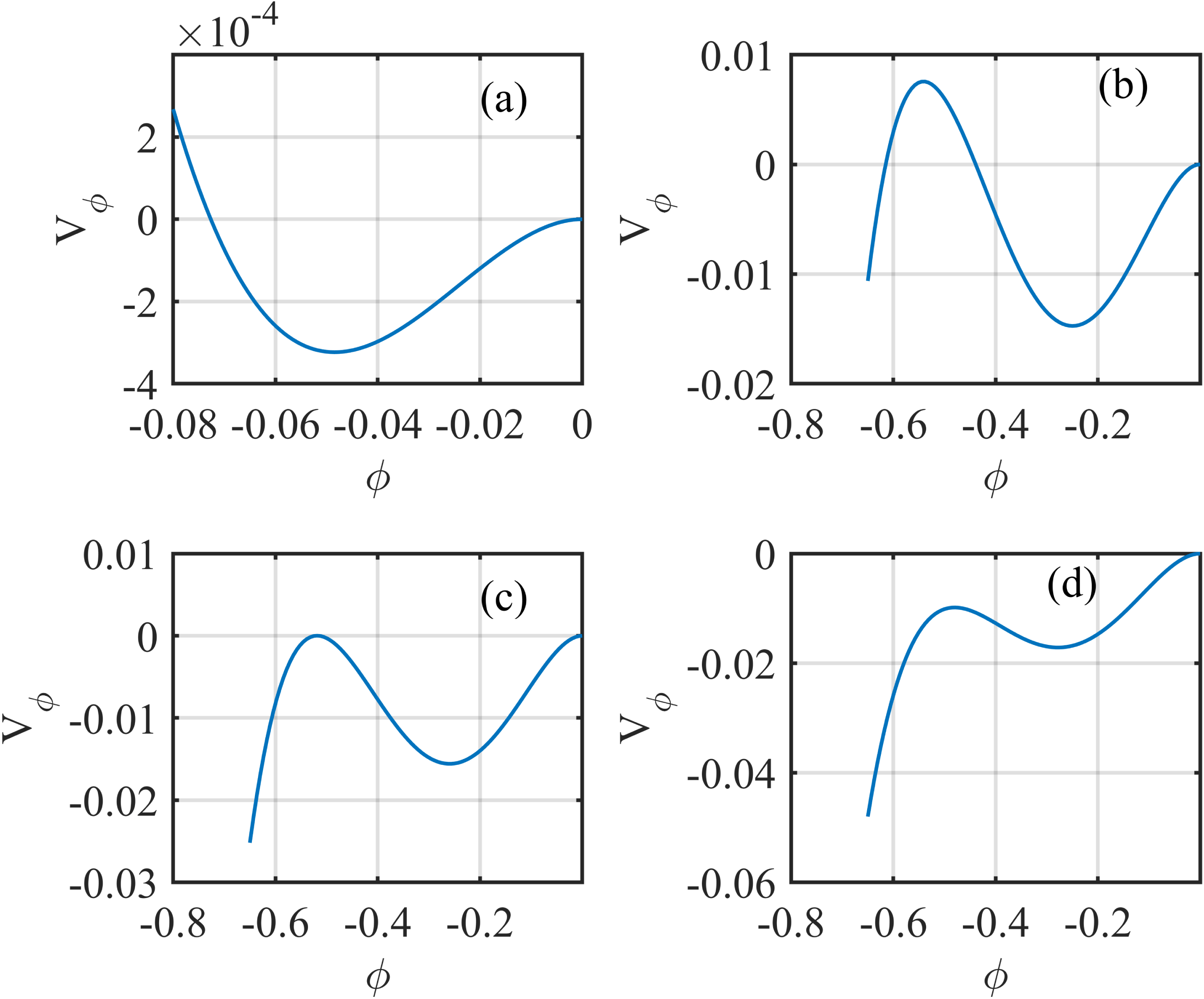
Sagdeev potential profiles for different Mach values leading to a transition from soliton to double layer. The parameters used are
 $\unicode[STIX]{x1D6FC}=0.1,\unicode[STIX]{x1D70E}_{h}=0.2,\unicode[STIX]{x1D705}_{i}=2.0,\unicode[STIX]{x1D705}_{e}=1.6$
with (a)
 $M/M_{s}=1.1181$
, (b)
 $M/M_{s}=1.3438$
, (c)
 $M/M_{s}=1.3469$
and (d)
 $M/M_{s}=1.3519$
.

If
 $M$
is increased above
 $M_{s}$
, solitons with increasing amplitude are formed until
 $M$
reaches an upper limit. Beyond this limit, no soliton can exist. This upper limit of
 $M$
may be because the perturbed density for a specific species vanishes, tends to infinity or become complex. Alternatively, this limiting value of
 $M$
may be due to the occurrence of a double layer. This statement will be clarified from figure 2, where the Sagdeev potential
 $V(\unicode[STIX]{x1D6F7})$
has been plotted with respect to
 $\unicode[STIX]{x1D6F7}$
for four different values of
 $M$
for a typical set of values of the compositional parameters
 $\unicode[STIX]{x1D6FC},\unicode[STIX]{x1D70E}_{h},\unicode[STIX]{x1D705}_{i}$
and
 $\unicode[STIX]{x1D705}_{e}$
. For this case,
 $\unicode[STIX]{x1D6FC}=0.1,\unicode[STIX]{x1D70E}_{h}=0.2,\unicode[STIX]{x1D705}_{i}=2.0$
and
 $\unicode[STIX]{x1D705}_{e}=1.6$
, and the value of
 $M_{s}$
is 0.5773. The values of
 $M$
in each of the cases are such that,
 $M/M_{s}=1.1181$
(figure 2
a),
 $M/M_{s}=1.3438$
(figure 2
b),
 $M/M_{s}=1.3469$
(figure 2
c) and
 $M/M_{s}=1.3519$
(figure 2
d). Here, it has been intended to illustrate the transition process from soliton to double layer with increasing Mach number. The first two figures (figures 2
a, 2
b) represent solitons, the third figure (figure 2
c) represents a double layer while the double layer disappear in the fourth figure (figure 2
d). All of the Sagdeev potential profiles have one local extremum excluding the endpoints. In figure 2(a,b), it crosses zero ensuring the recurrence of the initial state
 $V(0),V^{^{\prime }}(0)=0$
. In figure 2(c), the potential tends to the maximum amplitude where the solution transits to another state, the double layer. On further increase of the Mach value, in figure 2(d), the second root vanishes indicating the disappearance of the double layer.
Thus, for the generation of a double layer, there is another lower limit of Mach number which is also the upper limit for the soliton. It can be calculated from the condition
 $B_{3}>0$
. From the condition, it has been obtained that,
 $$\begin{eqnarray}\displaystyle M & {>} & \displaystyle \left[\left(\frac{(1+\unicode[STIX]{x1D6FC})(4\unicode[STIX]{x1D705}_{i}^{2}-1)(2\unicode[STIX]{x1D705}_{i}+3)}{6(2\unicode[STIX]{x1D705}_{i}-3)^{3}}+\frac{\unicode[STIX]{x1D6FC}(4\unicode[STIX]{x1D705}_{e}^{2}-1)(2\unicode[STIX]{x1D705}_{e}+3)}{6\unicode[STIX]{x1D70E}_{h}^{3}(2\unicode[STIX]{x1D705}_{e}-3)^{3}}\right)^{-1}\right.\nonumber\\ \displaystyle & & \displaystyle \times \left\{\frac{4}{3}\left(\frac{(1+\unicode[STIX]{x1D6FC})(4\unicode[STIX]{x1D705}_{i}^{2}-1)}{2(2\unicode[STIX]{x1D705}_{i}-3)^{2}}-\frac{\unicode[STIX]{x1D6FC}(4\unicode[STIX]{x1D705}_{e}^{2}-1)}{2\unicode[STIX]{x1D70E}_{h}^{2}(2\unicode[STIX]{x1D705}_{e}-3)^{2}}\right)\right.\nonumber\\ \displaystyle & & \displaystyle -\left.\!\left.\frac{1}{2}\left(\frac{(1+\unicode[STIX]{x1D6FC})(2\unicode[STIX]{x1D705}_{i}-1)}{(2\unicode[STIX]{x1D705}_{i}-3)}+\frac{\unicode[STIX]{x1D6FC}(2\unicode[STIX]{x1D705}_{e}-1)}{\unicode[STIX]{x1D70E}_{h}(2\unicode[STIX]{x1D705}_{e}-3)}\right)^{2}\right\}\right]^{1/2}=M_{dl}.\end{eqnarray}$$
Where
 $M_{dl}$
is the lower limit of the Mach number for the generation of the double layers. For
 $M\leqslant M_{dl}$
no double layer will exist. Thus the range
 $M_{s}-M_{dl}$
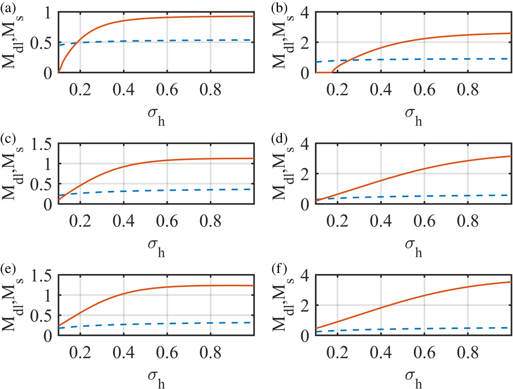
sets a range for the presence of solitons in the plasma. In figure 3, the existence domains for solitons and double layers are depicted for different sets of parameters. In the figure, (a,c,e) is for
 $\unicode[STIX]{x1D705}_{e}=1.6,\unicode[STIX]{x1D705}_{i}=2.0$
(superthermal electrons and ions) and (b,d,f) is for
 $\unicode[STIX]{x1D705}_{e}=100.0,\unicode[STIX]{x1D705}_{i}=100.0$
(Maxwellian electrons and ions). On the other hand, (a,b), (c,d) and (e,f) represent the existence domains for
 $\unicode[STIX]{x1D6FC}=0.5,\unicode[STIX]{x1D6FC}=1$
and
 $\unicode[STIX]{x1D6FC}=1.5$
respectively. In each of the plots, the dashed line represents the variation of
 $M_{s}$
with
 $\unicode[STIX]{x1D70E}_{h}$
, and the solid line represents that of
 $M_{dl}$
with
 $\unicode[STIX]{x1D70E}_{h}$
. The area between the two lines will provide the allowed value of Mach number for solitons. For DLs, the value of
 $M$
must be greater than the values above the solid line.
From the figure, it has been observed that for some cases, there are regions of the Mach number where the lower limit for solitons is greater than the lower limit for double layers, which does not correspond to a physical situation. The values of
 $M_{dl}$
for those regions are also found to be imaginary. Hence, no double layer will be generated for the values of
 $\unicode[STIX]{x1D70E}_{h},\unicode[STIX]{x1D6FC}$
and
 $\unicode[STIX]{x1D705}$
(both
 $\unicode[STIX]{x1D705}_{e},\unicode[STIX]{x1D705}_{i}$
) lying within that region. Further investigation implies that for the generation of the double layers, either the concentration of the hot electron component should be higher than that of the cold one or the electron to ion temperature ratio must be higher. It has to be noted that the minimum value of the Mach number required for the generation of the double layer is higher for Maxwellian particles, than that for the superthermal particles.
Existence diagram in Mach number space versus temperature ratio for different values of
 $\unicode[STIX]{x1D705}_{e},\unicode[STIX]{x1D705}_{i}$
, and
 $\unicode[STIX]{x1D6FC}$
. (a,c,e) is for superthermal electrons and ions
 $(\unicode[STIX]{x1D705}_{e}=3.0,\unicode[STIX]{x1D705}_{i}=2.0)$
and (b,d,f) is for Maxwellian electrons and ions
 $(\unicode[STIX]{x1D705}_{e}=100.0,\unicode[STIX]{x1D705}_{i}=100.0)$
. (a,b) is for
 $\unicode[STIX]{x1D6FC}=0.5$
, (c,d):
 $\unicode[STIX]{x1D6FC}=1.0$
and the (e,f):
 $\unicode[STIX]{x1D6FC}=1.5$
. The curve coding in each panel is: (a)
 $M_{s}$
dashed line, (b)
 $M_{dl}$
solid line.

3.3 The electron acoustic double layers
The nature and size of the electron acoustic double layers generated in the plasma can be studied with the help of (2.30). From this equation, it has been observed that, for the generation of the double layers,
 $B_{3}$
must be greater than 0. Since the amplitude of the double layers is expressed as
 $\unicode[STIX]{x1D713}=2B_{2}/3B_{3}$
, hence the sign of
 $B_{2}$
will indicate the polarity of the double layers. For a positive double layer
 $B_{2}>0$
and vice versa. Likewise, it has already been established that the sign of
 $V^{^{\prime \prime \prime }}(0,M_{s})$
determines the sign of the Kortewegde–Vries (KdV)-like solitons (solitons whose amplitude tends to 0 as
 $M\rightarrow M_{s}$
) (Verheest, Hellberg & Kourakis Reference Verheest, Hellberg and Kourakis2013). If the compositional parameters allow for
 $V^{^{\prime \prime \prime }}(0,M_{s})$
to go through zero and change sign, the polarity of the KdV-like solitary structures will change. From (2.29), it has been observed that
 $V^{^{\prime \prime \prime }}(0,M)=B_{2}$
. Coupling both of the conditions, finally the sign of
 $V^{^{\prime \prime \prime }}(0,M_{s})$
has been checked to gather ideas about the polarity of the solitary structures or to study how the compositional parameters alter of polarity of those structures. Here,
 $$\begin{eqnarray}\displaystyle V^{^{\prime \prime \prime }}(0,M_{s}) & = & \displaystyle \frac{(1+\unicode[STIX]{x1D6FC})(4\unicode[STIX]{x1D705}_{i}^{2}-1)}{2(2\unicode[STIX]{x1D705}_{i}-3)^{2}}-\frac{\unicode[STIX]{x1D6FC}(4\unicode[STIX]{x1D705}_{e}^{2}-1)}{2\unicode[STIX]{x1D70E}_{h}^{2}(2\unicode[STIX]{x1D705}_{e}-3)^{2}}\nonumber\\ \displaystyle & & \displaystyle -\,\frac{3}{2M_{s}^{2}}\left[\frac{(1+\unicode[STIX]{x1D6FC})(2\unicode[STIX]{x1D705}_{i}-1)}{(2\unicode[STIX]{x1D705}_{i}-3)}+\frac{\unicode[STIX]{x1D6FC}(2\unicode[STIX]{x1D705}_{e}-1)}{\unicode[STIX]{x1D70E}_{h}(2\unicode[STIX]{x1D705}_{e}-3)}\right].\end{eqnarray}$$
The relation,
 $V^{^{\prime \prime \prime }}(0,M_{s})=0$
can be solved numerically for
 $\unicode[STIX]{x1D6FC}$
(or any other parameter, e.g.
 $\unicode[STIX]{x1D70E}_{h}$
) to get the value for the critical density ratio
 $\unicode[STIX]{x1D6FC}_{c}$
(or
 $\unicode[STIX]{x1D70E}_{h_{\text{critical}}}$
) by keeping the values of the other parameters constant. For
 $\unicode[STIX]{x1D6FC}>\unicode[STIX]{x1D6FC}_{c}$
, positive KdV-like solitons will be generated and vice versa. Here, with
 $\unicode[STIX]{x1D70E}_{h}=0.2,\unicode[STIX]{x1D705}_{e}=3.0$
and
 $\unicode[STIX]{x1D705}_{i}=2.0$
, its value has been found to be
 $-$
0.0446, which is unphysical. To put things in perspective,
 $V^{^{\prime \prime \prime }}(0,M_{s})=0$
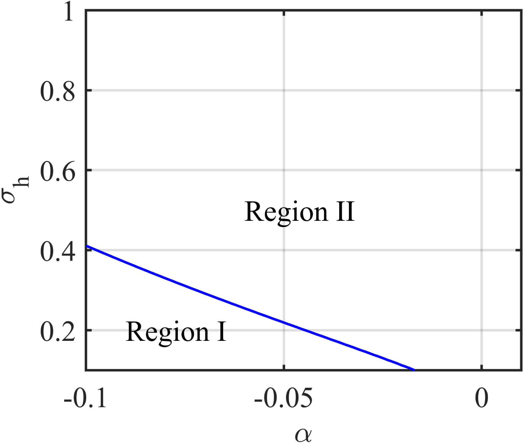
has been computed and the two regions (region for solitons with positive polarity, and region for those of negative polarity) are separated (figure 4). In the figure, the two regions are separated with the solid line. The area above the line (Region II) is for compressive KdV-like solitons (Baluku et al.
Reference Baluku, Hellberg, Kourakis and Saini2010; Verheest & Hellberg Reference Verheest and Hellberg2010) while the area below the line (Region I) is for rarefactive KdV-like solitons. For the values of the coordinates
 $(\unicode[STIX]{x1D6FC},\unicode[STIX]{x1D70E}_{h})$
lying above (below) the line, one can get compressive (rarefactive) KdV-like solitons. From the figure, it has been observed that negative KdV-like solitons have a chance of occurrence only for
 $-$
ve values of
 $\unicode[STIX]{x1D6FC}$
, which is not possible. In fact, the region for compressive solitons comprises some negative valued
 $\unicode[STIX]{x1D6FC}$
also. Thus, it is clear that for the allowed values of
 $\unicode[STIX]{x1D6FC}$
and
 $\unicode[STIX]{x1D70E}_{h}$
, the KdV-like soliton will be of only positive polarity.
The variation of the density fraction
 $(\unicode[STIX]{x1D6FC})$
, with temperature ratio
 $(\unicode[STIX]{x1D70E}_{h})$
, along the curve
 $V^{^{\prime \prime \prime }}(0,M_{s})=0$
across which the polarity changes. Above this curve (Region II),
 $V^{^{\prime \prime \prime }}(0,M_{s})>0$
(KdV-like solitons are positive), and below the curve (Region I)
 $V^{^{\prime \prime \prime }}(0,M_{s})<0$
(KdV-like solitons are negative). Other parameters are
 $\unicode[STIX]{x1D705}_{i}=2.0,\unicode[STIX]{x1D705}_{e}=3.0$
.

As already mentioned, the polarity of the double layers can be determined from the condition
 $B_{2}=0$
. If
 $B_{2}>0$
, the double layer will be compressive while it will be rarefactive if
 $B_{2}<0$
. Solving,
 $B_{2}=0$
, it has been observed that for some typical sets of values of
 $(\unicode[STIX]{x1D6FC},\unicode[STIX]{x1D70E}_{h})$
the zeros of
 $B_{2}$
can be achieved. This has been plotted in figure 5, where
 $B_{2}=0$
has been solved for two values of Mach number
 $(M)$
in the
 $\unicode[STIX]{x1D6FC}-\unicode[STIX]{x1D70E}_{h}$
space. The Mach values considered are,
 $M=1.1$
, and
 $M=2.0$
. The values of the other compositional parameters are
 $\unicode[STIX]{x1D705}_{i}=2.0$
, and
 $\unicode[STIX]{x1D705}_{e}=3.0$
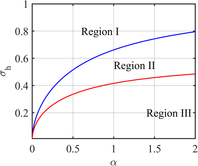
. In the figure, the ‘red line’ divides the two regions of positive and negative polarity double layers for
 $M=1.1$
, whereas the ‘blue line’ is for
 $M=2.0$
. From the figure, it is clear that with different values of the Mach number, the polarity of the double layer for the same values of the other compositional parameters can be different. For values of
 $\unicode[STIX]{x1D6FC}$
, and
 $\unicode[STIX]{x1D70E}_{h}$
located above the blue line, compressive double layers have been formed for both
 $M=1.1$
and
 $2.0$
(Region I). Similarly, for values of
 $\unicode[STIX]{x1D6FC}$
and
 $\unicode[STIX]{x1D70E}_{h}$
located below the red line, rarefactive double layers have been formed for both
 $M=1.1$
, and
 $2.0$
(Region III). Interestingly, for the region within the two lines, both positive
 $(M=1.1)$
and negative
 $(M=2.0)$
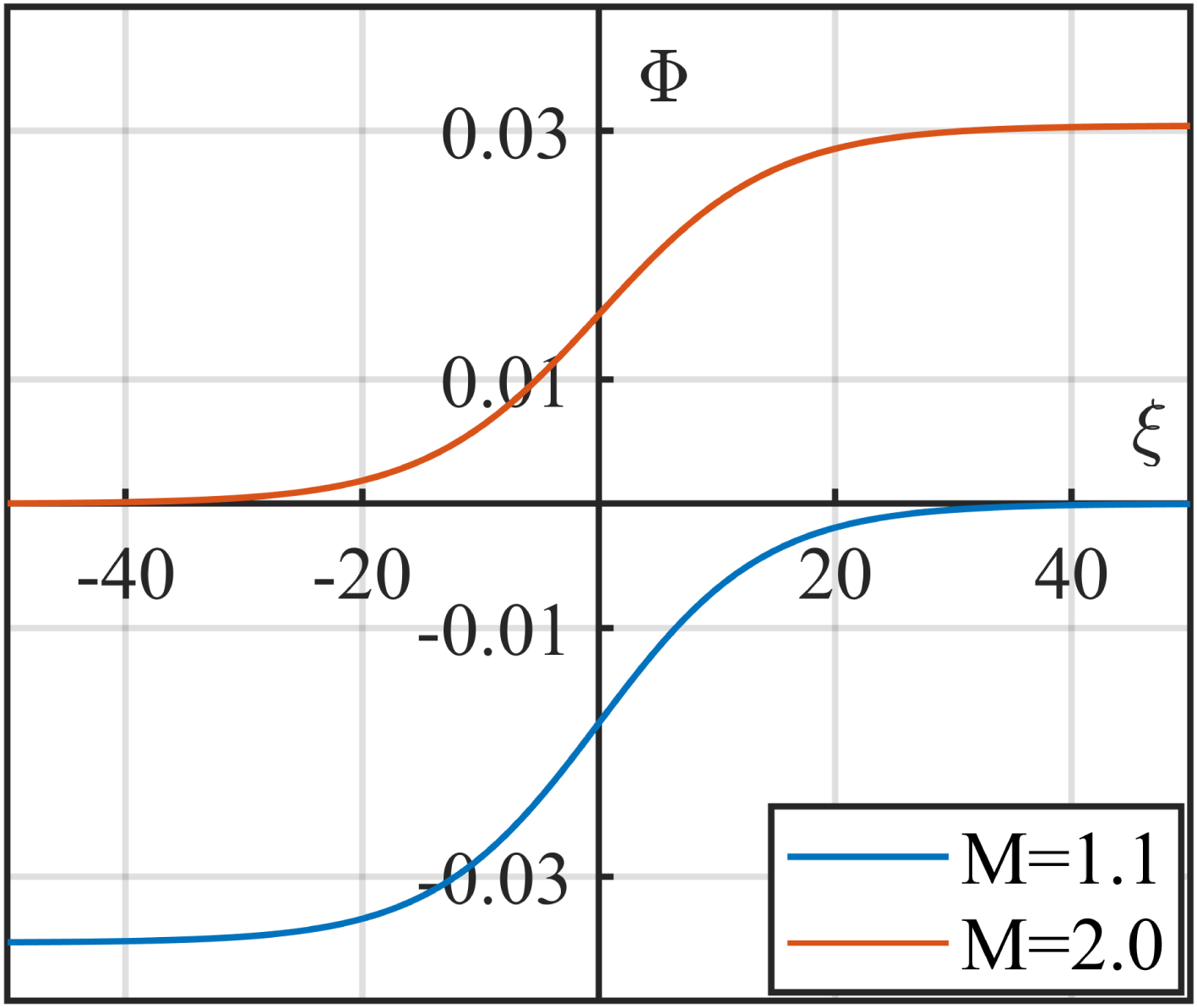
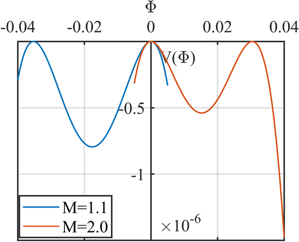
double layers have been generated (Region II). Thus, the polarity depends not only on the density and temperature ratio, but upon the Mach number too. The way of choosing the Mach number can alter the polarity of the double layers. The potential profile for the double layers along with its corresponding Sagdeev potential profile are plotted in figures 6 and 7 for two different values of
 $M$
.
The variation of the density fraction
 $(\unicode[STIX]{x1D6FC})$
, with temperature ratio
 $(\unicode[STIX]{x1D70E}_{h})$
, along the curve,
 $B_{2}=0$
across which the polarity changes. Above the curve
 $B_{2}>0$
, (positive double layers), and below the curve
 $B_{2}<0$
(negative double layers). The curve coding is: (a)
 $M=1.1$
(red line), and (b)
 $M=2.0$
(blue line). The region coding is: (a)
 $B_{2}(M=1.1)>0,~B_{2}(M=2.0)>0$
(Region I), (b)
 $B_{2}(M=1.1)<0,B_{2}(M=2.0)>0$
(Region II), (c)
 $B_{2}(M=1.1)<0,B_{2}(M=2.0)<0$
(Region III).

The potential profile of the double layer for Mach number
 $M=2.0$
(upper plot, red line), and
 $M=1.1$
(lower plot, blue line), with
 $\unicode[STIX]{x1D6FC}=0.1,\unicode[STIX]{x1D70E}_{h}=0.2,l_{z}=0.005,\unicode[STIX]{x1D705}_{e}=3.0$
and
 $\unicode[STIX]{x1D705}_{i}=2$
.

The Sagdeev potential profile of the double layer for Mach number
 $M=2.0$
(right-hand side, red line), and
 $M=1.1$
(left-hand side, blue line) with
 $\unicode[STIX]{x1D6FC}=0.1,\unicode[STIX]{x1D70E}_{h}=0.2,l_{z}=0.005,\unicode[STIX]{x1D705}_{e}=3.0$
and
 $\unicode[STIX]{x1D705}_{i}=2.0$
.

From figures 6 and 7, it has been observed that double layers with both positive and negative potential can exist in a plasma with the same compositional parameters, moving with two different velocities. In both of the figure, the blue line represents the double layers travelling with a Mach velocity
 $M=1.1$
, and the red line represents those with Mach velocity
 $M=2.0$
. The other parameters used here are,
 $\unicode[STIX]{x1D6FC}=0.4,\unicode[STIX]{x1D70E}_{h}=0.2,\unicode[STIX]{x1D705}_{i}=2.0$
and
 $\unicode[STIX]{x1D705}_{e}=3.0$
. To justify the results,
 $B_{2}=0$
has been solved for
 $M$
, with the same set of values of the other parameters. Solving numerically, it has been obtained that, at
 $M=M_{\text{critical}}=1.3526$
,
 $B_{2}=0$
. For
 $M>M_{\text{critical}}$
, positive double layers will form whereas for
 $M<M_{\text{critical}}$
, negative double layers will form. This result is analogous to the results obtained from figures 5–7.
3.4 The effect of the superthermal parameters on the amplitude and width of the double layers
The effect of the superthermal parameters
 $(\unicode[STIX]{x1D705},\unicode[STIX]{x1D70E}_{h},\unicode[STIX]{x1D6FC})$
on the nature and size of the double layers has also been studied here. For the observation, three different sets of spectral indices are chosen for the superthermal ions viz.
 $\unicode[STIX]{x1D705}_{i}=1.6$
(extremely superthermal ions),
 $\unicode[STIX]{x1D705}_{i}=2.0$
(superthermal ions) and
 $\unicode[STIX]{x1D705}_{i}=100$
(Maxwell–Boltzmann distributed ions). Similarly, three different sets of spectral indices are chosen for the superthermal electrons viz.
 $\unicode[STIX]{x1D705}_{e}=1.6$
(extremely superthermal electrons),
 $\unicode[STIX]{x1D705}_{e}=3.0$
(superthermal electrons) and
 $\unicode[STIX]{x1D705}_{e}=100$
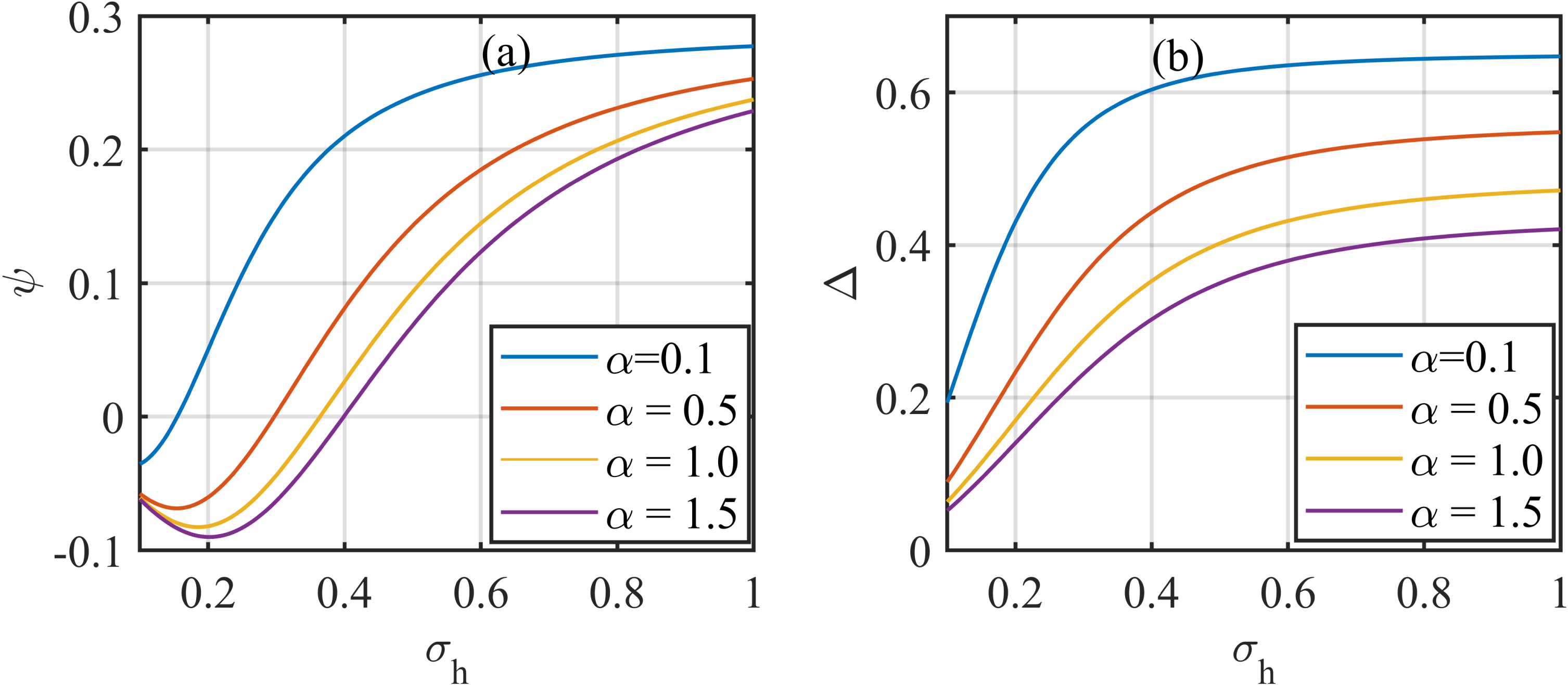
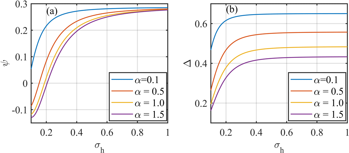
(Maxwell–Boltzmann distributed electrons). The variations of the amplitude
 $(\unicode[STIX]{x1D713})$
and the width
 $(\unicode[STIX]{x1D6E5})$
of the double layer with the temperature ratio
 $(\unicode[STIX]{x1D70E}_{h})$
are depicted in figure 8(a,b) respectively for
 $\unicode[STIX]{x1D705}_{e}=3.0$
, and
 $\unicode[STIX]{x1D705}_{i}=2.0$
. The value of
 $\unicode[STIX]{x1D70E}_{h}$
is varied from
 $0.1$
to
 $1.0$
. For
 $\unicode[STIX]{x1D70E}_{h}=0.1$
,
 $T_{i}=10T_{eh}$
whereas for
 $\unicode[STIX]{x1D70E}_{h}=1.0$
,
 $T_{i}=T_{eh}$
. The density ratio of the cold to hot electron components may also alter the nature of the double layer. So, the variations of the amplitude and width of the double layer have been observed for four different values of
 $\unicode[STIX]{x1D6FC}$
and are,
 $\unicode[STIX]{x1D6FC}=0.1$
,
 $\unicode[STIX]{x1D6FC}=0.5$
,
 $\unicode[STIX]{x1D6FC}=1.0$
and
 $\unicode[STIX]{x1D6FC}=1.5$
.
(a) The possible range of
 $\unicode[STIX]{x1D713}$
versus the temperature ratio
 $\unicode[STIX]{x1D70E}_{h}$
, (b) the possible range of
 $\unicode[STIX]{x1D6E5}$
versus the temperature ratio
 $\unicode[STIX]{x1D70E}_{h}$
. The parameters used are:
 $\unicode[STIX]{x1D705}_{e}=3.0,\unicode[STIX]{x1D705}_{i}=1.6,M=2.0,l_{z}=0.005$
.

(a) The possible range of
 $\unicode[STIX]{x1D713}$
versus the temperature ratio
 $\unicode[STIX]{x1D70E}_{h}$
, (b) the possible range of
 $\unicode[STIX]{x1D6E5}$
versus the temperature ratio
 $\unicode[STIX]{x1D70E}_{h}$
. The parameters used are:
 $\unicode[STIX]{x1D705}_{e}=100.0,\unicode[STIX]{x1D705}_{i}=2.0,M=7.0,l_{z}=0.005$
.

From the figure, it has been observed, depending upon the values of the different parameters, that both positive and negative double layers can exist, as mentioned earlier. It has been observed that, initially, the amplitude of the double layers decreases with an increase in the temperature ratio; except for
 $\unicode[STIX]{x1D6FC}=0.1$
. After attaining the minimum value, the double layer changes its polarity and the amplitude increases gradually with an increase in
 $\unicode[STIX]{x1D70E}_{h}$
. On the other hand, the width of the double layer increases with an increase in the temperature ratio. With an increase in the density ratio, both the amplitude as well as the width decrease.
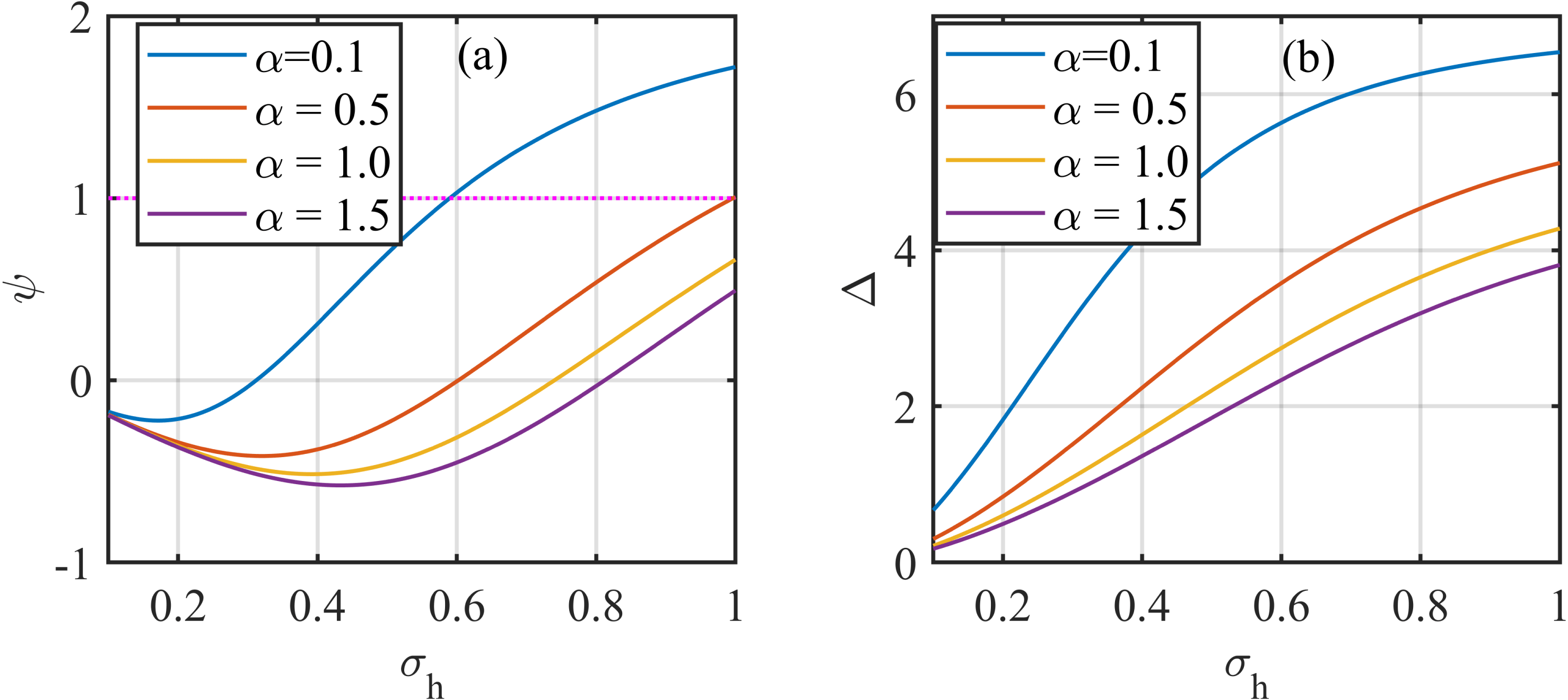
The effect of Maxwellian electrons has been observed in figure 9 where the variation in the amplitude (figure 9
a) and width (figure 9
b) of the double layer with the temperature ratio have been plotted for different concentrations of the electron components. The parameters used here are similar to the previous case except
 $\unicode[STIX]{x1D705}_{e}$
. This time
 $\unicode[STIX]{x1D705}_{e}=100.0$
. From the figure, it has been observed that both positive and negative double layers may exist in the plasma. The amplitude and width of the double layers increase with the increase in the temperature ratio. This increment is more prominent for lower values of
 $\unicode[STIX]{x1D70E}_{h}$
. On increasing the value of
 $\unicode[STIX]{x1D6FC}$
, the amplitude and width of the double layers decrease.
(a) The possible range of
 $\unicode[STIX]{x1D713}$
versus the temperature ratio
 $\unicode[STIX]{x1D70E}_{h}$
, (b) the possible range of
 $\unicode[STIX]{x1D6E5}$
versus the temperature ratio
 $\unicode[STIX]{x1D70E}_{h}$
. The parameters used are:
 $\unicode[STIX]{x1D705}_{e}=1.6,\unicode[STIX]{x1D705}_{i}=1.6,M=2.0,l_{z}=0.005$
.

(a) The possible range of
 $\unicode[STIX]{x1D713}$
versus the temperature ratio
 $\unicode[STIX]{x1D70E}_{h}$
, (b) the possible range of
 $\unicode[STIX]{x1D6E5}$
versus the temperature ratio
 $\unicode[STIX]{x1D70E}_{h}$
. The parameters used are:
 $\unicode[STIX]{x1D705}_{e}=100.0,\unicode[STIX]{x1D705}_{i}=100.0,M=7.5,l_{z}=0.005$
.

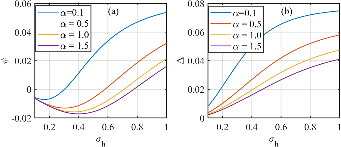
The variations in the amplitude and width of the double layer due to the presence of extremely superthermal electrons and ions (figure 10
a,b) as well as due to the presence of Maxwellian electrons and ions (figure 11
a,b) have been studied thereafter. For extremely superthermal electrons and ions,
 $\unicode[STIX]{x1D705}_{i}=\unicode[STIX]{x1D705}_{e}=1.6$
. In this case also, both amplitude and width increase with an increase in the value of
 $\unicode[STIX]{x1D70E}_{h}$
, while both decrease with an increase in the values of
 $\unicode[STIX]{x1D6FC}$
. The presence of compressive and rarefactive double layers can be verified from figure 10(a).
(a) The possible range of
 $\unicode[STIX]{x1D713}$
versus the temperature ratio
 $\unicode[STIX]{x1D70E}_{h}$
, (b) the possible range of
 $\unicode[STIX]{x1D6E5}$
versus the temperature ratio
 $\unicode[STIX]{x1D70E}_{h}$
. The parameters used are:
 $\unicode[STIX]{x1D705}_{e}=1.6,\unicode[STIX]{x1D705}_{i}=2.0,M=2.0,l_{z}=0.005$
.

Similar conclusions have been drawn from figure 11(a,b), featuring Maxwellian electrons and ions. However, from figure 11(a), it has been observed that for a smaller value of the ratio of concentration, the amplitude may exceed the allowed range of values (i.e.
 $\unicode[STIX]{x1D713}\ll 1$
) for
 $\unicode[STIX]{x1D70E}_{h}>0.6$
. Thus, in a plasma containing Maxwellian electrons and ions, double layers would be generated only for some particular values of
 $\unicode[STIX]{x1D6FC}$
and
 $\unicode[STIX]{x1D70E}_{h}$
.
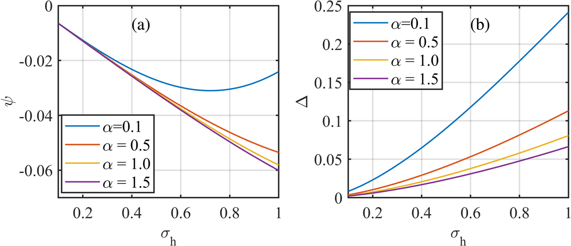
Suppose the hot electron component is more superthermal than the ions. To make a note on the effect of more superthermal electrons,
 $\unicode[STIX]{x1D705}_{e}$
has been considered to be
 $1.6$
, while
 $\unicode[STIX]{x1D705}_{i}=2.0$
. It has been observed that only rarefactive double layers would be generated in this case. Both the amplitude and width of the double layers have been observed to increase with an increase in the temperature ratio. The amplitude of the double layers in the presence of these plasma particles will increase with an increase in the density ratio, whereas the width will decrease with it. Therefore, from figures 9–12 the range of
 $\unicode[STIX]{x1D713},\unicode[STIX]{x1D6E5}$
versus
 $\unicode[STIX]{x1D70E}_{h}$
has been plotted for different compositions of the superthermal particles. From the figures it has been perceived that the plasma can sustain rarefactive double layers for lower values of the temperature ratio and compressive double layers for its higher values. However, when the hot component of electrons is more superthermal than the ions, only rarefactive double layers may be generated. On other hand, the width of the double layer increases with an increase in
 $\unicode[STIX]{x1D70E}_{h}$
, while it decreases with the increase in the concentration of the hot component of the electrons.
3.5 The variation of the values of the amplitude and velocity of the double layer with different values of the parameters
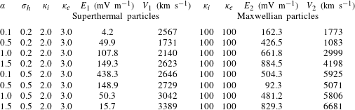
The amplitude and speed of the double layers obtained from this theoretical work are listed in table 1 for different values of the parameters. In the table, E1 and V1 are the amplitude and speed of the double layer in the presence of superthermal electrons and ions
 $(\unicode[STIX]{x1D705}_{i}=2.0,\unicode[STIX]{x1D705}_{e}=3.0)$
while E2 and V2 are those for Maxwellian electrons and ions
 $(\unicode[STIX]{x1D705}_{e}=\unicode[STIX]{x1D705}_{i}=100)$
. For the calculation, the assumed values of
 $\unicode[STIX]{x1D70E}_{h}$
are;
 $\unicode[STIX]{x1D70E}_{h}=0.2,0.5$
. Similarly, four values of
 $\unicode[STIX]{x1D6FC}$
have been considered here and are;
 $\unicode[STIX]{x1D6FC}=0.1,0.5,1.0,1.5$
. It has been mentioned earlier that the Van Allen Probe spacecraft detected a large number of different nonlinear structures, including double layers travelling at approximately
 $3100~\text{km}~\text{s}^{-1}$
along the magnetic field in the outer radiation belt. The peak amplitude of the double layers has been observed to be
 $30~\text{mV}~\text{m}^{-1}$
. For some particular values of the superthermal parameters, the amplitude and speed of the double layers obtained from this theoretical work have also been observed to be almost equal to the observed values.
Variation of the values of the electric field (
 $E_{1}$
,
 $E_{2}$
) and velocity (
 $V_{1}$
,
 $V_{2}$
) of the double layer with different values of the parameters.

4 Conclusion
In this work, the existence of electron acoustic double layers in a magnetized plasma consisting of superthermal electrons and ions along with cold fluid electrons has been investigated. The linear analysis of the governing equations leads to a dispersion relation, from which electron acoustic waves have been observed within the particular ordering of the parameters. The waves propagate in a direction almost perpendicular to the magnetic field (here,
 $\unicode[STIX]{x1D703}=89.7$
), with a phase velocity lower than
 $v_{T_{i}}$
and
 $v_{T_{eh}}$
.
From the nonlinear analysis, the existence domain for the solitary structures in terms of Mach number is evaluated. Employing different conditions on the Sagdeev pseudo-potential
 $V(\unicode[STIX]{x1D6F7})$
, required for the generation of nonlinear solitary structures, it has been observed that only compressive solitons can exist in the proposed plasma model. Further observations reveal that both compressive and rarefactive double layers can be generated in the modelled plasma. As already mentioned in § 3.3, the nature of the double layers depends on the density ratio of the hot to cold components of the electrons
 $(\unicode[STIX]{x1D6FC})$
, their temperature ratio
 $(\unicode[STIX]{x1D70E}_{h})$
as well as on the Mach velocity with which the nonlinear structures travel. Similarly, the amplitude of the double layers will depend upon
 $\unicode[STIX]{x1D6FC}$
, and
 $\unicode[STIX]{x1D70E}_{h}$
. The degree of superthermality of the electrons
 $(\unicode[STIX]{x1D705}_{e})$
and ions
 $(\unicode[STIX]{x1D705}_{i})$
can also alter the amplitude and polarity of the double layers.
Such a type of wave and the corresponding nonlinear structures are available in different space environments. Space-based experimental studies have already detected the signature of these electron acoustic waves. As mentioned in the previous sections (§§ 1 and 3.5), the observed electron acoustic double layers in the outer radiation belt reported by Mozer et al. (Reference Mozer, Bale, Bonnell, Chaston, Roth and Wygant2013) have peak amplitude
 $30~\text{mV}~\text{m}^{-1}$
and travel with a speed of approximately
 $3100~\text{km}~\text{s}^{-1}$
along the magnetic field lines. These double layers have been supposed to evolve from the electron acoustic wave generated in the plasma, which has been considered to be analogous to the ion acoustic wave except that the cold electrons play the role of cold ions to provide the inertia. They had assumed that the waves were generated by the instability associated with a whistler wave. In addition, they also mentioned the observation of double layers with an amplitude of almost
 $400~\text{mV}~\text{m}^{-1}$
by another Van Allen Probe observation. The double layers obtained from our theoretical work have also been observed to be of almost equal amplitude and speed for some particular values of the parameters. As the plasma model considered as well as the results obtained in our case are similar to those available in the outer radiation belt, the conclusions drawn from this study regarding the nature of the double layers will be helpful in understanding the dynamics of the waves in such space environments. Besides the radiation belt, the double layers generated in other space plasmas, for example bow shock, plasma sheet, magnetotail region of the Earth’s magnetosphere etc., can be explained with the theory of electron acoustic double layers deduced in this work.
It has been proposed that parametric instability can lead to the generation of double layers in some space plasma environments. Hence, this work has a further scope of the study of the generation of electron acoustic double layers in a magnetized plasma due to instability. The effect of Landau damping on the evolution of such double layers is another interesting topic planned to be studied later.