2.1. Structural analysis

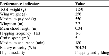
Birds in nature have complex wing structures that enable them to make complex maneuvers during takeoff, hunting, and evasion of predators. However, due to material and structural design limitations, the current FWFR wings do not have the same degree of freedom as birds. At present, the FWFRs with high flight efficiency still mainly use single-degree-of-freedom flapping wings, such as the Dovelike FWFR [Reference Yang, Wang and Song22], which set the Guinness World Record for single-charge flight endurance of FWFR in 185 minutes. The LFWFR studied in this paper is based on our research on the high-efficiency LFWFR platform HIT-Hawk. The main performance parameters are shown in Table I.

Table I.

HIT-Hawk main specification.

HIT-Hawk adopted a modular approach in the overall mechanical design, as shown in Figure 1. It is mainly divided into four parts: fuselage module, transmission module, tail module, and wing module. The body is cut from a carbon fiber board and used to connect various modules. The transmission module converts the rotation of the brushless direct current motor (BLDC) into reciprocating flapping of wings through a two-stage gear reducer. The flapping wing is connected to the fuselage through a ball head, providing the main lift and thrust for flight. There are two servos on the tail to control the attitude of HIT-Hawk.

Figure 1.

The structural design diagram of HIT-Hawk.

The wings are composed of carbon fiber composite rods and lightweight membrane materials, which are glued to the skeleton. The mass of the unloaded HIT-Hawk is 1150 g, while the mass of the wings is 256 g, accounting for 22.26% of the total weight of HIT-Hawk. The wing/body mass ratio for avian is a range of 10–20%. The 22.26% wing/body mass ratio is near the large flapping-wing avians like eagles or albatrosses. Reference [Reference Sibilski, Loroch, Buler and Zyluk23] pointed out that ignoring the inertia force of flapping wings may lead to different or even completely incorrect results in dynamics and control problems, which is particularly evident for LFWFRs. Therefore, the influence of inertial force cannot be ignored when calculating loads. Considering the coupling of aerodynamic, inertial, and elastic forces during flapping, it is necessary to establish structural dynamic equations for LFWFR wings.

2.2. Modeling

The large flexible deformation and high proportion of flapping wing mass of LFWFRs result in a strong coupling relationship between wing aerodynamic loads and structural deformation. Therefore, in the aerodynamic calculation of flexible flapping wings, the flexible deformation of the flapping wings needs to be considered, and correspondingly, the influence of aerodynamic loads also needs to be taken into account in the deformation calculation of flexible flapping wings. To this end, we calculate the aerodynamic loads and structural deformations of flexible flapping wings based on finite state aerodynamic models and equivalent wing structure dynamic models and exchange data between aerodynamic and structural nodes through radial basis functions (RBF) [Reference Yang, Song, Yang, Xue, Pei and Lang18]. Finally, we use the Newmark method to solve the dynamic equations. The model framework is shown in Figure 2.

Figure 2.

Aeroelastic dynamics model framework.

The flapping equation of the wings is derived from the spatial crank connecting rod mechanism model of the transmission module [Reference Zhong and Xu24], and the flapping equation obtained through third-order Fourier fitting is:

(1) \begin{equation} \beta =a_{0}+\sum _{i=1}^{3}\left(a_{i}\cos \left(\frac{i\cdot f}{2}t\right)+b_{i}\sin \left(\frac{i\cdot f}{2}t\right)\right) \end{equation}

where $\beta$ is the flapping angle (rad), $f$ is the flapping frequency, $a_{0}=0.2362 , a_{1}=-0.3818 , b_{1}=0.00686 , a_{2}=0.03003 , b_{2}=-0.001706 , a_{3}=-0.003558 , b_{3}= 0.0002689$ . When $t=0$ , the flapping wing is at the highest position.

3.1. Aerodynamic model

The aerodynamic model established in this section is based on the two-dimensional finite state airloads theory derived by Peters et al. [Reference Peters, Hsieh and Torrero25]. This theory is based on the assumption of incompressible potential flow, which can be coupled with any unsteady wake model to calculate the aerodynamic loads of thin airfoils under large rigid motions and small deformations. The incompressible potential flow assumption applies to the situation of low-speed flow, high Reynolds number, and no flow separation. The flight velocity of LFWFRs is much lower than 100 m/s (0.3 times the speed of sound). The Reynolds numbers Re > 10⁶ and AOA < 20°, which are not prone to flow separation. Thus, the two-dimensional finite state airloads theory is suitable for LFWFRs aerodynamic analysis. Compared with the computational fluid dynamics (CFD) method, the calculation speed of this method is much faster. Using the same computer, the CFD method often takes more than 10 h to complete the calculation of one flapping cycle, while this method takes less than 1 s. Furthermore, this method can be coupled with the structural dynamics equations and multi-body dynamics equations, which is applicable to the design of control laws for LFWFRs.

A thin airfoil wing of arbitrary shape undergoing unsteady motion in two-dimensional space is considered. A Cartesian coordinate system is established as shown in Figure 3. The origin of the coordinate system is defined at the midpoint of the chord length of the airfoil. The air velocity in the $x$ positive direction is $u_{0}$ , the air velocity in the $y$ positive direction is $v_{0}$ , and the velocity gradient of the overall rotation of the coordinate system is $v_{1}$ . If counterclockwise is defined as positive, then the vertical velocity of the airfoil at the horizontal $x$ axis can be expressed as $v_{0}+v_{1}x/b$ , where $b$ is the half chord length of the airfoil. The rigid motion of the airfoil is characterized by $u_{0} , v_{0}$ , and $v_{1}$ . The deformation is represented by the mid-curve deformation function $h(x,t)$ (positive down). The deformation of the airfoil is much smaller than the motion in the coordinate system so that $h\ll b , \partial h/\partial x\ll 1$ and $\partial h/\partial t\ll u_{0}$ . Then the nonpenetration condition of the thin airfoil can be written as [Reference Peters, Hsieh and Torrero25]:

(2) \begin{equation} w=\overline{v}+\lambda =u_{0}\partial h/\partial x+\partial h/\partial t+v_{0}+v_{1}x/b \end{equation}

where $w$ is the total induced flow, $\lambda$ is the induced flow from the trailed circulation, and $\overline{v}$ is the induced flow from bound circulation.

Figure 3.

Two-dimensional airfoil flapping diagram within a flapping cycle (leftwing).

Let $\varphi =\arccos (x/b)$ , Glauert expansions are used for $h$ :

(3) \begin{equation} h=\sum _{n=0}^{N_{aero}}h_{n}\cos \left(n\varphi \right) \end{equation}

where $N_{aero}$ is the order of Glauert expansion. In this paper, we set $N_{aero}=6$ . The expansion parameter $h_{n}$ can be calculated by:

(4) \begin{equation} \boldsymbol{h}_{\boldsymbol{n}}=\boldsymbol{T}_{\boldsymbol{g}}\cdot \boldsymbol{h}_{\boldsymbol{\varphi }} \end{equation}

(5) \begin{equation} \boldsymbol{T}_{\boldsymbol{g}}=\left[\begin{array}{c@{\quad}c@{\quad}c@{\quad}l} 1 & 1 & 1 & \cdots \\ \cos \left(\varphi _{1}\right) & \cos \left(\varphi _{2}\right) & \cos \left(\varphi _{3}\right) & \cdots \\ \cos \left(2\varphi _{1}\right) & \cos \left(2\varphi _{2}\right) & \cos \left(2\varphi _{3}\right) & \cdots \\ \vdots & \vdots & \vdots & \ddots \end{array}\right] \end{equation}

where $\boldsymbol{T}_{\boldsymbol{g}}$ is a $(N_{aero}+1)\times N_{\textit{guass}}$ matrix. $\boldsymbol{h}_{\boldsymbol{\varphi }}$ is the deformation of each Gauss point. The position of each Gauss point is defined by Gauss–Chebyshev Quadrature Formula. The number of Guass point $N_{\textit{gauss}}$ in each airfoil is 7. The pressure distribution ${\unicode[Arial]{x0394}} P$ in each Guass point can be expanded as [Reference Peters, Hsieh and Torrero25]:

(6) \begin{equation} {\unicode[Arial]{x0394}} P\left(\varphi \right)=2\rho \left[\frac{\tau _{s}}{\sin \varphi }-\frac{\tau _{0}\cos \varphi }{\sin \varphi }+\sum _{n=1}^{\infty }\tau _{n}\sin \left(n\varphi \right)\right] \end{equation}

For forward flight two-dimensional airfoil, $\tau _{s}=\tau _{0}$ . $\rho$ is the air density. The expansion terms are written as [Reference Stanford, Beran and Kobayashi26]:

(7) \begin{equation} \begin{aligned} \boldsymbol{\tau }_{\boldsymbol{n}}&=u_{0}\left(\boldsymbol{v}_{\boldsymbol{n}}-\boldsymbol{\lambda }_{\boldsymbol{0}}\right)+\left(b\boldsymbol{W}_{\boldsymbol{aero}}\cdot \dot{\boldsymbol{v}}_{\boldsymbol{n}}/2\right)\\ &\quad+\left(u_{0}^{2}\boldsymbol{I}_{\boldsymbol{n}}/b+\dot{u}_{0}\boldsymbol{W}_{\boldsymbol{aero}}/2\right)\cdot \boldsymbol{K}_{\boldsymbol{aero}}\cdot \boldsymbol{h}_{\boldsymbol{n}}\\ &\quad +u_{0}\left(\boldsymbol{I}_{\boldsymbol{n}}+\boldsymbol{W}_{\boldsymbol{aero}}\cdot \boldsymbol{K}_{\boldsymbol{aero}}/2\right)\cdot \dot{\boldsymbol{h}}_{\boldsymbol{n}}+b\boldsymbol{W}_{\boldsymbol{aero}}\cdot \ddot{\boldsymbol{h}}_{\boldsymbol{n}}/2 \end{aligned} \end{equation}

where the vectors $\boldsymbol{v}_{\boldsymbol{n}}=\{\begin{array}{l@{\quad}l@{\quad}l@{\quad}l@{\quad}l} v_{0} & v_{1} & 0 & \ldots & 0 \end{array}\}^{T}$ and $\boldsymbol{\lambda }_{\boldsymbol{0}}=\{\begin{array}{l@{\quad}l@{\quad}l@{\quad}l@{\quad}l} \lambda _{0} & 0 & 0 & \ldots & 0 \end{array}\}^{T}$ . $\boldsymbol{I}_{\boldsymbol{n}}$ is the identity matrix. $\boldsymbol{W}_{\boldsymbol{aero}}$ and $\boldsymbol{K}_{\boldsymbol{aero}}$ could be obtained from ref. [Reference Stanford, Beran and Kobayashi26]. Similarly, Eq. (6) could also be put in matrix form:

(8) \begin{equation} \boldsymbol{\unicode{x1D6E5} }\boldsymbol{P}=2\rho \boldsymbol{P}_{\boldsymbol{g}}\cdot \boldsymbol{\tau }_{\boldsymbol{n}} \end{equation}

(9) \begin{equation} \boldsymbol{P}_{\boldsymbol{g}}=\left[\begin{array}{l@{\quad}l@{\quad}l@{\quad}l}\displaystyle \frac{1-\cos \left(\varphi _{1}\right)}{\sin \left(\varphi _{1}\right)} & \sin \left(\varphi _{1}\right) & \sin \left(2\varphi _{1}\right) & \cdots \\ \\ \displaystyle\frac{1-\cos \left(\varphi _{2}\right)}{\sin \left(\varphi _{2}\right)} & \sin \left(\varphi _{2}\right) & \sin \left(2\varphi _{2}\right) & \cdots \\ \\ \displaystyle\frac{1-\cos \left(\varphi _{3}\right)}{\sin \left(\varphi _{3}\right)} & \sin \left(\varphi _{3}\right) & \sin \left(2\varphi _{3}\right) & \cdots \\ \vdots & \vdots & \vdots & \ddots \end{array}\right] \end{equation}

The aerodynamic loads along the x and y axes in the airfoil coordinate system are as follows:

(10) \begin{equation} \begin{aligned} F_{x}&=\int _{-b}^{b}{\Delta} P\left(\frac{\partial h}{\partial x}\right)\,\text{d}x-2\pi b\rho \left(v_{0}+\dot{h}_{0}-\lambda _{0}+u_{0}\sum _{n=1,3,5}^{\infty }nh_{n}/b\right)^{2}\\ F_{y}&=\int _{-b}^{b}{\Delta} P\,\text{d}x \end{aligned} \end{equation}

To solve the above equation, the first term of Glauert expansion of the induced flow $\lambda _{0}$ (i.e., the uniform inflow) should be obtained. Based on the extended least squares method, $\lambda _{0}$ can be calculated by the weighted sum of inflow states:

(11) \begin{equation} \lambda _{0}\approx \frac{1}{2}\sum _{n=1}^{N}b_{n}\lambda _{n} \end{equation}

The calculation method of $b_{n}$ and $\lambda _{n}$ can be referred to ref. [Reference Peters, Arunamoorthyt and Cao27]. $N$ is the number of inflow states. It should be noted that the aerodynamic loads obtained by the above method is two-dimensional. For a three-dimensional flapping wing, the aerodynamic load of the whole wing can be obtained by the blade element theory along the spanwise direction. This theory ignores the spanwise flow, which only applies to high aspect ratio (AR) wings (AR>5 is better [Reference Li, Yu, Lin and Li28]).

3.2. Structural model

The finite element method is one of the most commonly used methods for calculating structural deformation, which is widely used in the flexible deformation calculation for various FWFRs [Reference Si, Hao, Guo, Tong and Bing29]. As mentioned in ref. [Reference Xue, Song, Song, Yang, Xu and Wu30], only the skeleton bears the air loads as long as there is no prestress on the membrane. Thus, it is feasible to establish the flapping-wing structural model that only considers the skeleton and distributes the mass of membrane on the skeleton to approximate the inertial effects of membrane. This model is established through beam elements in commercial finite element software Abaqus. The epoxy carbon fiber material used for the skeleton is anisotropic, and the material parameters can be obtained in ref. [Reference Liu, Liu and Ding31]. The global mass matrix and global stiffness matrix of the wing can be obtained from this finite element model.

The global damping matrix is determined by the Rayleigh damping method, which is simple, convenient, and widely used in structural dynamic analysis. The Rayleigh damping assumption assumes that the damping matrix of a structure is a combination of the mass matrix and stiffness matrix:

(12) \begin{equation} \boldsymbol{C}=a\boldsymbol{M}+b\boldsymbol{K} \end{equation}

In (12), $a$ and $b$ are the proportional coefficients, which can be determined by the natural frequencies and damping ratio. The natural frequency can be obtained from the Abaqus structural model, and the damping ratio can be determined from the loss factor of the material. For HIT-Hawk, the values of $a$ and $b$ are 0.037 and 0.0005, respectively.

The motion equation of each structural node on the wing of a LFWFR can be simplified as:

(13) \begin{equation} \boldsymbol{M}\cdot \ddot{\boldsymbol{h}}\boldsymbol{=}\boldsymbol{C}\cdot \dot{\boldsymbol{q}}\boldsymbol{+}\boldsymbol{K}\cdot \boldsymbol{q}\boldsymbol{+}\boldsymbol{F}_{aero} \end{equation}

where $\boldsymbol{h}$ is the displacement function of the node, $\boldsymbol{q}$ is the structural deformation of the wing node, $\boldsymbol{M}$ is the global mass matrix of the wing, $\boldsymbol{K}$ is the global stiffness matrix, and $\boldsymbol{C}$ is the global damping matrix. Let the rigid displacement of the wing node be $\boldsymbol{\zeta }$ . We can get:

(14) \begin{equation} \boldsymbol{\zeta }\boldsymbol{=}\boldsymbol{q}\boldsymbol{+}\boldsymbol{h} \end{equation}

For wing movements with known flapping equations, the rigid flapping motion of the wings can be used to characterize $\boldsymbol{\zeta }$ . Considering that there is no aerodynamic load in a vacuum environment, $\boldsymbol{F}_{\boldsymbol{aero}}$ can be ignored, substituting Eq. (14) into Eq. (13) yields:

(15) \begin{equation} \boldsymbol{M}\cdot \ddot{\boldsymbol{q}}\boldsymbol{+}\boldsymbol{K}\cdot \boldsymbol{q}\boldsymbol{+}\boldsymbol{C}\cdot \dot{\boldsymbol{q}}\boldsymbol{=}\boldsymbol{M}\cdot \ddot{\boldsymbol{\zeta }} \end{equation}

Equation (15) can be solved using numerical analysis methods such as mode superposition method or the Newmark method. Here, the Newmark method is chosen as the average constant acceleration method, assuming that the acceleration at each time step is continuous, and its value is the average acceleration at the beginning and end of the time step ( $\gamma =0.5 , \beta =0.25$ ). When the time step ${\unicode[Arial]{x0394}} t$ is less than 0.001s, the calculation is convergent. The deformation $\boldsymbol{q}_{\boldsymbol{t}\boldsymbol{+}\boldsymbol{\Delta}\boldsymbol{t}}$ amount and its velocity $\dot{\boldsymbol{q}}_{\boldsymbol{t}\boldsymbol{+}\boldsymbol{\Delta }\boldsymbol{t}}$ at $t+\Delta t$ can be calculated using the following two equations:

(16) \begin{equation} \boldsymbol{q}_{\boldsymbol{t}\boldsymbol{+}\boldsymbol{\Delta }\boldsymbol{t}}=\boldsymbol{q}{\boldsymbol{t}}+\Delta t\dot{\boldsymbol{q}}_{\boldsymbol{t}}+\left(\frac{1}{2}-\beta \right)\left(\Delta t\right)^{2}\ddot{\boldsymbol{q}}_{\boldsymbol{t}}+\beta \left(\Delta t\right)^{2}\ddot{\boldsymbol{q}}_{\boldsymbol{t}\boldsymbol{+}\boldsymbol{\varDelta }\boldsymbol{t}} \end{equation}

(17) \begin{equation} \dot{\boldsymbol{q}}_{\boldsymbol{t}\boldsymbol{+}\boldsymbol{\varDelta }\boldsymbol{t}}=\dot{\boldsymbol{q}}_{\boldsymbol{t}}+\left(1-\gamma \right)\Delta t\ddot{\boldsymbol{q}}_{\boldsymbol{t}}+\gamma \Delta t\ddot{\boldsymbol{q}}_{\boldsymbol{t}\boldsymbol{+}\boldsymbol{\varDelta }\boldsymbol{t}} \end{equation}

In $t+{\unicode[Arial]{x0394}} t$ :

(18) \begin{equation} \boldsymbol{M}\cdot \ddot{\boldsymbol{q}}_{\boldsymbol{t}\boldsymbol{+}\boldsymbol{\varDelta }\boldsymbol{t}}+\boldsymbol{C}\cdot \dot{\boldsymbol{q}}_{\boldsymbol{t}\boldsymbol{+}\boldsymbol{\varDelta }\boldsymbol{t}}+\boldsymbol{K}\cdot \boldsymbol{q}_{\boldsymbol{t}\boldsymbol{+}\boldsymbol{\varDelta }\boldsymbol{t}}=\boldsymbol{F}_{\boldsymbol{t}\boldsymbol{+}\boldsymbol{\varDelta }\boldsymbol{t}} \end{equation}

Combine Eq. (14), Eq. (15), and Eq. (16), we can get:

(19) \begin{equation} \hat{\boldsymbol{M}}\cdot \ddot{\boldsymbol{q}}_{\boldsymbol{t}\boldsymbol{+}\boldsymbol{\varDelta }\boldsymbol{t}}\boldsymbol{=}\hat{\boldsymbol{F}}_{\boldsymbol{t}\boldsymbol{+}\boldsymbol{\varDelta }\boldsymbol{t}} \end{equation}

where

(20) \begin{equation} \hat{\boldsymbol{M}}=\boldsymbol{M}+\gamma \Delta t\boldsymbol{C}+\beta \left(\Delta t\right)^{2}\boldsymbol{K} \end{equation}

(21) \begin{equation} \begin{aligned} \hat{\boldsymbol{F}}_{\boldsymbol{t}\boldsymbol{+}\boldsymbol{\varDelta }\boldsymbol{t}}&=\boldsymbol{M}\cdot \ddot{\boldsymbol{\zeta }}_{\boldsymbol{t}\boldsymbol{+}\boldsymbol{\varDelta }\boldsymbol{t}}-\boldsymbol{K}\cdot \boldsymbol{q}_{\boldsymbol{t}}-\left(\boldsymbol{C}+\Delta t\boldsymbol{K}\right)\cdot \dot{\boldsymbol{q}}_{\boldsymbol{t}}\\ &\quad -\left(\left(1-\gamma \right)\Delta t\boldsymbol{C}\left(\frac{1}{2}-\beta \right)\left(\Delta t\right)^{2}\boldsymbol{K}\right)\cdot \ddot{\boldsymbol{q}}_{\boldsymbol{t}} \end{aligned} \end{equation}

Therefore, as we set the deformation, deformation speed, and acceleration at the initial time, the deformation can be iteratively solved by Eq. (17). For calculation with aerodynamic loads, we just need to add $\boldsymbol{F}_{\boldsymbol{aero}}$ in Eq. (13). Since the discretization methods of aerodynamic and structural mesh are different, a corresponding conversion algorithm is needed to realize the data exchange between aerodynamic and structural mesh. In this paper, we choose a polynomial interpolation method based on RBFs.