1 Introduction
Electrophoresis of a charged particle suspended in a fluid electrolyte is now often studied within small scale microelectromechanical (MEMS) devices and nanopores, in part driven by interest in characterisation and separation of cells and molecules (Xuan, Raghibizadeh & Li Reference Xuan, Raghibizadeh and Li2006; Kang & Li Reference Kang and Li2009). If the flow device is a circular tube of radius
 $R$
and the particle a sphere of radius
 $a$
only slightly smaller than
 $R$
, the electric field within the narrow gap between the cylindrical wall of the tube and the surface of the sphere is much larger than that within the tube far from the particle. This high field facilitates the observation of nonlinear effects. Experiments (Tokarz et al. (Reference Tokarz, Hakonen, Dommersnes, Orwar and Ȧkerman2007); S. Tottori, private communication) have shown that electrophoresis of a sphere in a circular tube is nonlinear in the applied electric field strength
 $E_{0}$
. Here we shall provide a theoretical analysis of nonlinear electrophoretic motion confined within a rigid circular tube (rather than within the non-rigid lipid nanotube used by Tokarz et al. (Reference Tokarz, Hakonen, Dommersnes, Orwar and Ȧkerman2007)).
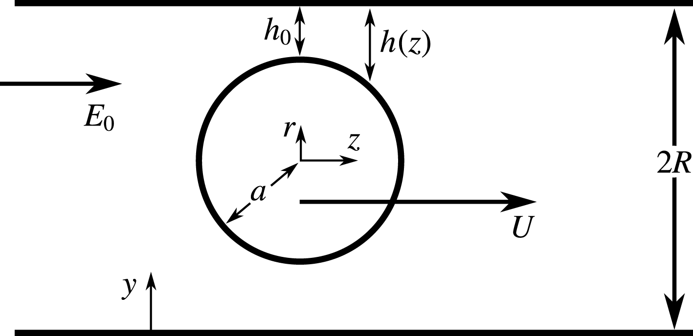
The sphere, of radius
 $a$
on the axis of a cylinder of internal radius
 $R=a+h_{0}$
. The imposed electric field has strength
 $E_{0}$
far from the sphere, and the electrophoretic velocity of the sphere is
 $U$
.

We consider a sphere of radius
 $a$
on the axis of a fluid-filled circular cylinder of radius
 $R=a+h_{0}$
(figure 1). The sphere is charged, with uniform surface charge density
 $\unicode[STIX]{x1D70E}_{s}$
, and the uniform surface charge density on the cylinder is
 $\unicode[STIX]{x1D70E}_{c}$
. The fluid within the cylindrical tube has viscosity
 $\unicode[STIX]{x1D707}$
and contains one species of cations (with charge
 $eZ$
, where
 $e$
is the charge on a proton) and one of anions (charge
 $-Ze$
), each with number density
 $n_{0}$
far from any charged surfaces. The charge clouds of counter-ions adjacent to the charged surfaces have thickness characterised by the Debye length
 $\unicode[STIX]{x1D705}^{-1}$
, with
 $$\begin{eqnarray}\displaystyle \unicode[STIX]{x1D705}^{2}=\frac{2Z^{2}e^{2}n_{0}}{\unicode[STIX]{x1D716}kT}, & & \displaystyle\end{eqnarray}$$
where
 $\unicode[STIX]{x1D716}$
is the permittivity of the fluid and
 $kT$
is the Boltzmann temperature.
The geometry is axisymmetric: we use cylindrical polar coordinates
 $(z,r)$
, with the
 $z$
axis aligned along the axis of the tube, and with the centre of the sphere on the plane
 $z=0$
. We shall also use
 $y$
as a generic coordinate normal to a solid surface, with
 $y>0$
in the fluid. Thus
 $y=R-r$
is a coordinate normal to the surface of the cylinder. A potential difference is applied across the ends of the tube, such that the electric field is
 $\boldsymbol{E}_{0}=E_{0}\hat{\boldsymbol{z}}$
within the tube far from the sphere.
One of the first analyses of electrophoresis of a sphere in a cylinder was that of Keh & Anderson (Reference Keh and Anderson1985) who used the method of reflections to determine the velocity of a sphere of radius
 $a\ll R$
on the cylinder axis, for the case of thin double layers
 $\unicode[STIX]{x1D705}a\gg 1$
. The applied field was weak, so that the velocity
 $U$
of the charged sphere (with surface potential
 $\unicode[STIX]{x1D701}_{s}$
) relative to the charged tube (surface potential
 $\unicode[STIX]{x1D701}_{c}$
) was linear in the imposed field
 $E_{0}$
and proportional to
 $(\unicode[STIX]{x1D701}_{s}-\unicode[STIX]{x1D701}_{c})$
as long as the ends of the tube were open, so that no pressure-driven backflow was generated. Keh & Chiou (Reference Keh and Chiou1996) used numerical computations to determine the linear electrophoretic velocity of a sphere, surrounded by a thin double layer of thickness
 $\unicode[STIX]{x1D705}^{-1}\ll \min (a,h_{0})$
, on the axis of the cylinder for the full range of
 $a/R$
, and in the limit of a tightly fitting sphere found
 $$\begin{eqnarray}\displaystyle U=\unicode[STIX]{x1D716}E_{0}(\unicode[STIX]{x1D701}_{s}-\unicode[STIX]{x1D701}_{c})/2\unicode[STIX]{x1D707},\quad R-a\ll R. & & \displaystyle\end{eqnarray}$$
Further numerical work by Hsu & Chen (Reference Hsu and Chen2007) and Chiu & Keh (Reference Chiu and Keh2016) allowed for relaxation of the charge cloud. Yariv & Brenner (Reference Yariv and Brenner2002) extended the analysis of Keh & Anderson (Reference Keh and Anderson1985) to predict the linear electrophoretic velocity of a small sphere off the axis of the cylinder, and full numerical computations were reported by Ye, Xuan & Li (Reference Ye, Xuan and Li2005). Yariv & Brenner (Reference Yariv and Brenner2003) determined analytically the velocity of a tightly fitting sphere. Their analysis confirmed the earlier numerical result (1.2) for a sphere on the axis of the cylinder, and also predicted electrophoretic velocities for tightly fitting spheres off the axis. Thus previous work on electrophoresis in a circular cylinder has been restricted to analyses in which the electrophoretic velocity is proportional to the electric field. However, most of the above papers (with the exception of those of Ye et al. (Reference Ye, Xuan and Li2005) and Chiu & Keh (Reference Chiu and Keh2016)) assumed infinitesimally thin charge clouds. It has been shown (Schnitzer & Yariv Reference Schnitzer and Yariv2012c
) that when
 $a\unicode[STIX]{x1D705}\gg 1$
the Smoluchowski electrophoretic velocity
 $\unicode[STIX]{x1D716}\unicode[STIX]{x1D701}E_{0}/\unicode[STIX]{x1D707}$
of a sphere in unbounded fluid holds even for strong fields and moderate zeta potentials as long as the Dukhin number (which represents the ratio of surface conduction to bulk conduction, and will be defined in (1.3) below) is negligibly small. We might therefore expect the above analyses, linear in the applied electric field, to hold as long as the Dukhin number is negligibly small.
The mobile ions forming a charge cloud in fluid electrolyte adjacent to a charged surface move in response to gradients of electrochemical potential, and the resulting effective surface conductivity cannot be neglected if the number of ions in the charge cloud is sufficiently high. The electric field tangential to a curved surface is in general non-uniform, and conservation of ions requires fluxes of ions into or out of the charge cloud from or to the bulk electrolyte. These fluxes perturb the ionic concentration and electric potential in the bulk electrolyte. A uniform electric field of strength
 $E_{0}$
imposed on a spherical particle of radius
 $a$
suspended in electrolyte and surrounded by a thin double layer therefore creates a perturbation of the ionic concentration in the electrolyte.
If the imposed field is weak, with
 $\hat{E}_{0}=E_{0}ae/(kT)\ll 1$
, the leading-order perturbations to the ionic concentration and electric potential are dipoles (e.g. Schnitzer et al.
Reference Schnitzer, Zeyde, Yavneh and Yariv2013, equation (3.11)). These dipoles decay slowly on the length scale of the particle, and the change in the electric potential around the particle is thought to be the origin of the enhanced low-frequency electrical permittivity of dilute suspensions of charged particles (Dukhin & Shilov Reference Dukhin and Shilov1974; Fixman Reference Fixman1980; Hinch et al.
Reference Hinch, Sherwood, Chew and Sen1984).
The modification of the ionic concentration and potential caused by ionic fluxes into/out of the charge cloud has an effect upon the electrophoretic velocity of the particle (Schnitzer & Yariv Reference Schnitzer and Yariv2012b
), and nonlinear electrophoresis of a sphere with a thin double layer (
 $a\unicode[STIX]{x1D705}\gg 1$
) in unbounded fluid has been studied in various limiting cases. Schnitzer et al. (Reference Schnitzer, Zeyde, Yavneh and Yariv2013) assumed a weak electric field
 $\hat{E}_{0}\ll 1$
and used this as the basis for a perturbation expansion in order to find an
 $O(\hat{E}_{0}^{3})$
correction to the electrophoretic velocity. The convection–diffusion equation for ionic motion is singular, and had to be solved by matched asymptotic expansions. Results were given in terms of a Dukhin number
 $$\begin{eqnarray}\displaystyle Du={\displaystyle \frac{(1+2\unicode[STIX]{x1D6FC}_{-})}{a\unicode[STIX]{x1D705}}}{\displaystyle \frac{\unicode[STIX]{x1D70E}_{s}Ze}{\unicode[STIX]{x1D716}\unicode[STIX]{x1D705}kT}}=(1+2\unicode[STIX]{x1D6FC}_{-}){\displaystyle \frac{\unicode[STIX]{x1D70E}_{s}}{2aZen_{0}}}, & & \displaystyle\end{eqnarray}$$
where
 $\unicode[STIX]{x1D6FC}_{\pm }$
are related to the ionic mobilities
 $\unicode[STIX]{x1D714}_{\pm }$
by
 $$\begin{eqnarray}\displaystyle \unicode[STIX]{x1D6FC}_{\pm }={\displaystyle \frac{\unicode[STIX]{x1D716}kT}{e^{2}Z^{2}\unicode[STIX]{x1D707}\unicode[STIX]{x1D714}_{\pm }}}, & & \displaystyle\end{eqnarray}$$
as discussed in § 4 below. The Dukhin number represents the ratio of surface conduction to bulk conduction, and when it is vanishingly small the electrophoretic velocity of the sphere is given by the linear Smoluchowski velocity even at high imposed fields
 $\hat{E}_{0}\sim a\unicode[STIX]{x1D705}\gg 1$
(Schnitzer & Yariv Reference Schnitzer and Yariv2012c
). Schnitzer & Yariv (Reference Schnitzer and Yariv2014) considered the limit
 $Du\ll 1$
, and found the
 $O(Du)$
correction to the electrophoretic velocity as a function of
 $\hat{E}_{0}$
. For
 $\hat{E}_{0}$
small (typically less than 10) the correction was negative, but for large field strengths the correction was positive, increasing as
 $\hat{E}_{0}^{3/2}$
at high field strengths. Schnitzer & Yariv (Reference Schnitzer and Yariv2012a
) considered non-zero solid permittivity
 $\unicode[STIX]{x1D716}_{s}>0$
, and found nonlinear corrections to the electrophoretic velocity when
 $\hat{E}_{0}\unicode[STIX]{x1D716}_{s}/\unicode[STIX]{x1D716}$
is sufficiently large.
The aim of the analysis presented here is to determine the perturbation of the ionic number densities created by the fluxes of ions into and out of the charge clouds in the gap between the sphere and the cylindrical wall of the tube in the limit when the gap is narrow (
 $h_{0}=R-a\ll a$
), and to determine the corresponding change in the electrophoretic velocity of the sphere. To ensure that perturbations of ionic number densities are small, we shall require a non-dimensional number
 $S$
, related to the product
 $\hat{E}_{0}\,Du$
and defined in (4.22) of § 4, to be small. The Péclet number that characterises the ratio of ionic convection to diffusion will be required to be sufficiently small so that the ionic concentration across the narrow gap between the sphere and tube is approximately uniform. However, when the gap is narrow this is not an onerous restriction, as will be discussed in § 4.
The surface of the sphere is at
 $$\begin{eqnarray}\displaystyle r=r_{s}(z)=(a^{2}-z^{2})^{1/2} & & \displaystyle\end{eqnarray}$$
and so the width
 $h$
of the gap between the surface of the sphere and the wall of the cylinder can be approximated as
 $$\begin{eqnarray}\displaystyle h=R-r_{s}\approx h_{0}\left(1+\frac{z^{2}}{2ah_{0}}\right)=h_{0}\left(1+\frac{z^{2}}{\unicode[STIX]{x1D6FD}^{2}}\right), & & \displaystyle\end{eqnarray}$$
where
 $$\begin{eqnarray}\displaystyle \unicode[STIX]{x1D6FD}^{2}=2ah_{0}=2Rh_{0}\left(1-\frac{h_{0}}{R}\right). & & \displaystyle\end{eqnarray}$$
The cross-sectional area of the portion of the tube occupied by fluid is
 $$\begin{eqnarray}\displaystyle A\approx 2\unicode[STIX]{x03C0}Rh\approx 2\unicode[STIX]{x03C0}Rh_{0}\left(1+\frac{z^{2}}{\unicode[STIX]{x1D6FD}^{2}}\right). & & \displaystyle\end{eqnarray}$$
More generally, the shape of any spheroid (or any body of revolution with non-zero second derivative of
 $R(z)$
at
 $z=0$
) may be approximated by (1.6) for an appropriate value of
 $\unicode[STIX]{x1D6FD}$
. We shall therefore use
 $\unicode[STIX]{x1D6FD}$
throughout the analysis, rather than replacing it by
 $\unicode[STIX]{x1D6FD}=(2ah_{0})^{1/2}$
(1.7) which holds only for spheres.
We shall rely strongly upon the lubrication approximation, and neglect slow variations of
 $r_{s}(z)$
when computing the flow of fluid and ions. Thus, locally, flow takes place within a channel between walls separated by a distance
 $h$
, and of total (circular) width approximately
 $2\unicode[STIX]{x03C0}R$
. The electric field is similarly assumed to be unidirectional, corresponding to a potential
 $\unicode[STIX]{x1D719}$
that is a function only of
 $z$
. Fields in the radial direction will be
 $O(\text{d}h/\text{d}z)$
smaller than those in the axial direction. We assume that the permittivity
 $\unicode[STIX]{x1D716}_{s}$
of the solid surfaces is negligibly small. Non-zero solid permittivities lead to an electric field in the solid, and perturb the ionic number density in the charge cloud adjacent to the surface. The tangential electric field acting on the perturbed charge cloud may then lead to perturbed fluid velocities nonlinear in the applied electric field, and this can modify electrophoretic velocities when the Dukhin number is non-zero and the applied electric field is sufficiently strong (Schnitzer & Yariv Reference Schnitzer and Yariv2012a
). The ranges of validity of the various approximations are discussed by Schnitzer & Yariv (Reference Schnitzer and Yariv2014), and we leave non-zero
 $\unicode[STIX]{x1D716}_{s}$
as a subject for possible future study.
We assume that charge clouds are thin, i.e.
 $\unicode[STIX]{x1D705}^{-1}\ll h_{0}\ll R$
. Conservation of charge requires that the total current across any plane of constant
 $z$
should be independent of
 $z$
and hence, if the concentration of ions outside the charge clouds is uniform and we neglect any surface conductivity, the electric field within the gap between the sphere and the cylinder wall has magnitude (in the one-dimensional lubrication approximation)
 $$\begin{eqnarray}\displaystyle E=\frac{E_{0}\unicode[STIX]{x03C0}R^{2}}{A}\approx \frac{E_{0}R}{2h}=\frac{E_{0}R}{2h_{0}(1+z^{2}/\unicode[STIX]{x1D6FD}^{2})}. & & \displaystyle\end{eqnarray}$$
The electric potential
 $\unicode[STIX]{x1D719}$
within the gap satisfies
 $E=-\text{d}\unicode[STIX]{x1D719}/\text{d}z$
and is
 $$\begin{eqnarray}\displaystyle \unicode[STIX]{x1D719}=-\frac{E_{0}R\unicode[STIX]{x1D6FD}}{2h_{0}}\tan ^{-1}(z/\unicode[STIX]{x1D6FD}), & & \displaystyle\end{eqnarray}$$
so that the total drop in potential across the particle is
 $$\begin{eqnarray}\displaystyle [\unicode[STIX]{x1D719}]_{-\infty }^{\infty }=-\frac{E_{0}R\unicode[STIX]{x1D6FD}\unicode[STIX]{x03C0}}{2h_{0}}. & & \displaystyle\end{eqnarray}$$
We note that (1.9) and (1.10) are valid only within the narrowest part of the gap between the sphere and cylinder, where the parabolic approximation (1.6) for the gap width holds. We have not used the formal language of matched asymptotic expansions, but the above analysis for the electric field gives the leading-order inner expansion for the electric field in the narrowest part of the gap (cf. Yariv & Brenner Reference Yariv and Brenner2003; Yariv Reference Yariv2016b ).
The analysis presented in this paper draws directly from the ideas of Schnitzer & Yariv (Reference Schnitzer and Yariv2014), and we shall endeavour to show how it relates to their work. As in the linear electrophoresis analysis of Yariv & Brenner (Reference Yariv and Brenner2003) there are four length scales,
 $\unicode[STIX]{x1D705}^{-1}\ll h_{0}\ll \unicode[STIX]{x1D6FD}\ll R$
. We leave the equations in dimensional form: this allows dimensional analysis to be used as a check, and gives results that can immediately be compared to experiment. The price is more complex notation, and we shall sometimes non-dimensionalise potentials within the charge clouds by
 $kT/eZ$
, with the resulting non-dimensional quantity denoted by a caret, in order to simplify the typography.
We first (§ 2) recall the distribution of ions within an equilibrium electrical double layer, together with the fluid velocity generated by an externally applied tangential electric field. In § 3 we derive the standard leading-order (in
 $h/R$
) expression for the electrophoretic velocity of a tightly fitting sphere in a cylinder (Yariv & Brenner Reference Yariv and Brenner2003). The tangential convective and diffusive fluxes of ions within the double layers are obtained in appendix B. The flux of counter-ions can be large when the surface charge density on the solid surface is sufficiently high, and the effect of this flux upon the ionic concentration in the bulk solution is studied in § 4. In § 5 we determine the change in electrophoretic velocity caused by these perturbations.
2 The charge cloud adjacent to a uniformly charged plane
2.1 Equilibrium ionic distribution
We consider a charge cloud at equilibrium with bulk electrolyte in which the local ionic concentration (of both anions and cations) far from any charged surface is
 $n_{\infty }$
and the electrical potential is
 $\unicode[STIX]{x1D719}_{\infty }$
. The potential within the charge cloud is
 $\unicode[STIX]{x1D713}$
, and we set
 $$\begin{eqnarray}\displaystyle \hat{\unicode[STIX]{x1D711}}=\frac{Ze}{kT}(\unicode[STIX]{x1D713}-\unicode[STIX]{x1D719}_{\infty }), & & \displaystyle\end{eqnarray}$$
so that
 $\hat{\unicode[STIX]{x1D711}}$
is the (non-dimensional) potential relative to that far from the charged surface. At equilibrium, the number densities
 $n_{+}$
of cations and
 $n_{-}$
of anions are given by the Boltzmann distribution
 $$\begin{eqnarray}\displaystyle n_{+}=n_{\infty }\text{e}^{-\hat{\unicode[STIX]{x1D711}}},\quad n_{-}=n_{\infty }\text{e}^{\hat{\unicode[STIX]{x1D711}}}, & & \displaystyle\end{eqnarray}$$
and the potential is related to the charge density
 $\unicode[STIX]{x1D70C}$
by the Poisson equation
 $\unicode[STIX]{x1D6FB}^{2}\unicode[STIX]{x1D713}=-\unicode[STIX]{x1D70C}/\unicode[STIX]{x1D716}$
, so that
 $$\begin{eqnarray}\displaystyle \unicode[STIX]{x1D6FB}^{2}\hat{\unicode[STIX]{x1D711}}=\frac{Z^{2}e^{2}n_{\infty }}{\unicode[STIX]{x1D716}kT}(\text{e}^{\hat{\unicode[STIX]{x1D711}}}-\text{e}^{-\hat{\unicode[STIX]{x1D711}}})=\frac{\unicode[STIX]{x1D705}^{2}}{2}\frac{n_{\infty }}{n_{0}}(\text{e}^{\hat{\unicode[STIX]{x1D711}}}-\text{e}^{-\hat{\unicode[STIX]{x1D711}}}). & & \displaystyle\end{eqnarray}$$
If the charge cloud is thin compared with the radius of curvature of the charged surface, we may neglect curvature, and the solution of (2.3) for the equilibrium potential in the charge cloud, at a distance
 $y=\unicode[STIX]{x1D702}/\unicode[STIX]{x1D705}$
from a surface at potential
 $\unicode[STIX]{x1D701}+\unicode[STIX]{x1D719}_{\infty }$
, is
 $$\begin{eqnarray}\displaystyle \text{e}^{\hat{\unicode[STIX]{x1D711}}/2}={\displaystyle \frac{A+\text{e}^{-\unicode[STIX]{x1D702}B}}{A-\text{e}^{-\unicode[STIX]{x1D702}B}}}, & & \displaystyle\end{eqnarray}$$
where
 $$\begin{eqnarray}\displaystyle A={\displaystyle \frac{\text{e}^{\hat{\unicode[STIX]{x1D701}}/2}+1}{\text{e}^{\hat{\unicode[STIX]{x1D701}}/2}-1}},\quad B=\left(\frac{n_{\infty }}{n_{0}}\right)^{1/2}, & & \displaystyle\end{eqnarray}$$
and where
 $\unicode[STIX]{x1D701}$
is the potential at the surface
 $\unicode[STIX]{x1D702}=0$
relative to the potential
 $\unicode[STIX]{x1D719}_{\infty }$
outside the charge cloud. We assume that the Debye length
 $\unicode[STIX]{x1D705}^{-1}$
is sufficiently small compared to the gap width
 $h$
, so that the charge cloud on the surface of the sphere does not interact with that on the cylindrical surface of the tube. Each charge cloud is consequently described by (2.4) and (2.5), in terms of the appropriate zeta potential
 $\unicode[STIX]{x1D701}_{c}$
on the surface of the cylinder or
 $\unicode[STIX]{x1D701}_{s}$
on the sphere, and the appropriate local normal coordinate
 $y$
. The zeta potential
 $\unicode[STIX]{x1D701}$
is related to the surface charge density
 $\unicode[STIX]{x1D70E}$
by
 $$\begin{eqnarray}\displaystyle \unicode[STIX]{x1D70E}=-\unicode[STIX]{x1D716}\left.\frac{\unicode[STIX]{x2202}\unicode[STIX]{x1D713}}{\unicode[STIX]{x2202}y}\right|_{y=0} & = & \displaystyle 2\unicode[STIX]{x1D716}\unicode[STIX]{x1D705}B\frac{kT}{Ze}\sinh \left(\frac{\hat{\unicode[STIX]{x1D701}}}{2}\right)\end{eqnarray}$$
 $$\begin{eqnarray}\displaystyle & {\approx} & \displaystyle \unicode[STIX]{x1D716}\unicode[STIX]{x1D705}B\frac{kT}{Ze}\text{e}^{\hat{\unicode[STIX]{x1D701}}/2}\quad \text{if }\hat{\unicode[STIX]{x1D701}}\gg 1\end{eqnarray}$$
 $$\begin{eqnarray}\displaystyle & {\approx} & \displaystyle \unicode[STIX]{x1D716}\unicode[STIX]{x1D705}B\unicode[STIX]{x1D701}\quad \text{if }\hat{\unicode[STIX]{x1D701}}\ll 1.\end{eqnarray}$$
We assume (without loss of generality)
 $\unicode[STIX]{x1D70E}>0$
, so that the counter-ions in the charge cloud are anions, and the co-ions are cations.
2.2 The slip velocity
A tangential electric field
 $-\unicode[STIX]{x1D735}_{t}\unicode[STIX]{x1D719}_{\infty }$
or tangential gradient of ionic number density
 $\unicode[STIX]{x1D735}_{t}n_{\infty }$
outside the charge cloud creates fluid motion, and the fluid velocity relative to the charged plane, just outside the double layer (i.e. the slip velocity) is
 $$\begin{eqnarray}\displaystyle \boldsymbol{u}_{slip}=\frac{\unicode[STIX]{x1D716}\unicode[STIX]{x1D701}}{\unicode[STIX]{x1D707}}\unicode[STIX]{x1D735}_{t}\unicode[STIX]{x1D719}_{\infty }-\frac{4\unicode[STIX]{x1D716}(kT)^{2}}{\unicode[STIX]{x1D707}e^{2}Z^{2}}\ln [\cosh (\hat{\unicode[STIX]{x1D701}}/4)]\unicode[STIX]{x1D735}_{t}\ln n_{\infty }. & & \displaystyle\end{eqnarray}$$
For completeness we give a short derivation of this well-known result in appendix A.
The slip velocity will be perturbed if the electrical potential
 $\unicode[STIX]{x1D719}_{\infty }$
and ionic number density
 $n_{\infty }$
are perturbed. We suppose that
 $$\begin{eqnarray}\displaystyle \unicode[STIX]{x1D719}_{\infty }=\unicode[STIX]{x1D719}_{0}+\unicode[STIX]{x1D719}_{1}+\cdots \,,\quad n_{\infty }=n_{0}+n_{1}+\cdots \,, & & \displaystyle\end{eqnarray}$$
where
 $\unicode[STIX]{x1D719}_{1}$
and
 $n_{1}$
are small perturbations that will be determined in § 4.
If the surface charge density
 $\unicode[STIX]{x1D70E}$
is held constant, the change in ionic concentration causes a change in
 $\unicode[STIX]{x1D701}$
potential. To determine this change, we set
 $\unicode[STIX]{x1D701}=\unicode[STIX]{x1D701}_{0}+\unicode[STIX]{x1D701}_{1}+\cdots \,$
in (2.6) to obtain
 $$\begin{eqnarray}\displaystyle \sinh \left({\displaystyle \frac{\hat{\unicode[STIX]{x1D701}}_{0}}{2}}\right)+{\displaystyle \frac{\hat{\unicode[STIX]{x1D701}}_{1}}{2}}\cosh \left({\displaystyle \frac{\hat{\unicode[STIX]{x1D701}}_{0}}{2}}\right)={\displaystyle \frac{\unicode[STIX]{x1D70E}eZ}{2\unicode[STIX]{x1D716}\unicode[STIX]{x1D705}kT}}\left[1-{\displaystyle \frac{n_{1}}{2n_{0}}}\right], & & \displaystyle\end{eqnarray}$$
so that (Schnitzer & Yariv Reference Schnitzer and Yariv2014)
 $$\begin{eqnarray}\displaystyle \unicode[STIX]{x1D701}=\unicode[STIX]{x1D701}_{0}-{\displaystyle \frac{kT}{eZ}}\tanh \left({\displaystyle \frac{\hat{\unicode[STIX]{x1D701}}_{0}}{2}}\right){\displaystyle \frac{n_{1}}{n_{0}}}. & & \displaystyle\end{eqnarray}$$
The first-order perturbation to the slip velocity (2.9) therefore has magnitude
 $$\begin{eqnarray}\displaystyle u_{slip,1}=\frac{\unicode[STIX]{x1D716}\unicode[STIX]{x1D701}_{0}}{\unicode[STIX]{x1D707}}\frac{\unicode[STIX]{x2202}\unicode[STIX]{x1D719}_{1}}{\unicode[STIX]{x2202}z}-\frac{\unicode[STIX]{x1D716}kT}{\unicode[STIX]{x1D707}eZ}\tanh \left(\frac{\hat{\unicode[STIX]{x1D701}}_{0}}{2}\right)\frac{n_{1}}{n_{0}}\frac{\unicode[STIX]{x2202}\unicode[STIX]{x1D719}_{0}}{\unicode[STIX]{x2202}z}-\frac{4\unicode[STIX]{x1D716}k^{2}T^{2}}{\unicode[STIX]{x1D707}e^{2}Z^{2}n_{0}}\ln \left[\cosh \left(\frac{\hat{\unicode[STIX]{x1D701}}_{0}}{4}\right)\right]\frac{\unicode[STIX]{x2202}n_{1}}{\unicode[STIX]{x2202}z}, & & \displaystyle\end{eqnarray}$$
where we note that
 $\unicode[STIX]{x1D735}n_{0}=0$
.
3 Electrophoresis: low applied field
The charge densities
 $\unicode[STIX]{x1D70E}_{c}$
and
 $\unicode[STIX]{x1D70E}_{s}$
on the surface of the cylinder and sphere are assumed to be uniform. At leading order the ionic concentration
 $n=n_{\infty }=n_{0}$
is uniform outside the charge clouds, and so the zeta potentials
 $\unicode[STIX]{x1D701}=\unicode[STIX]{x1D701}_{s}$
on the spherical particle and
 $\unicode[STIX]{x1D701}=\unicode[STIX]{x1D701}_{c}$
on the cylindrical wall are uniform and related to the charge density by (2.6). The Smoluchowski slip velocity (2.9) at the surface of the charged sphere has magnitude
 $$\begin{eqnarray}\displaystyle u_{s}=-{\displaystyle \frac{\unicode[STIX]{x1D716}\unicode[STIX]{x1D701}_{s}}{\unicode[STIX]{x1D707}}}E={\displaystyle \frac{U_{s}R}{2h}}, & & \displaystyle\end{eqnarray}$$
where
 $$\begin{eqnarray}\displaystyle U_{s}=-{\displaystyle \frac{\unicode[STIX]{x1D716}\unicode[STIX]{x1D701}_{s}E_{0}}{\unicode[STIX]{x1D707}}} & & \displaystyle\end{eqnarray}$$
is the slip velocity corresponding to the unperturbed electric field far from the particle. The slip velocity on the inner surface of the cylinder is
 $$\begin{eqnarray}\displaystyle u_{c}=-{\displaystyle \frac{\unicode[STIX]{x1D716}\unicode[STIX]{x1D701}_{c}}{\unicode[STIX]{x1D707}}}E={\displaystyle \frac{U_{c}R}{2h}}, & & \displaystyle\end{eqnarray}$$
where
 $$\begin{eqnarray}\displaystyle U_{c}=-{\displaystyle \frac{\unicode[STIX]{x1D716}\unicode[STIX]{x1D701}_{c}E_{0}}{\unicode[STIX]{x1D707}}}. & & \displaystyle\end{eqnarray}$$
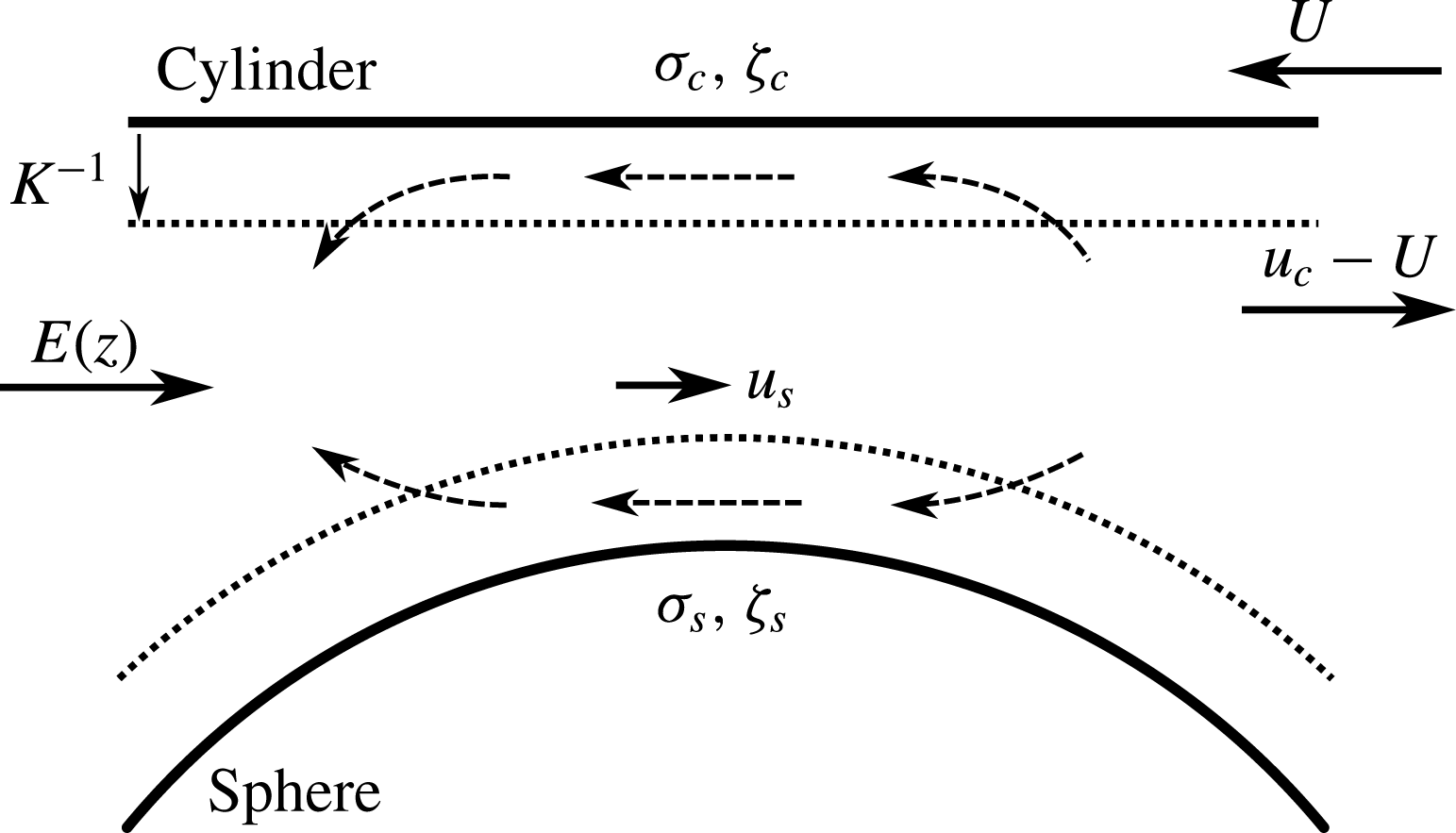
The velocity
 $-U$
of the cylindrical wall, and slip velocities
 $u_{s}$
and
 $u_{c}-U$
in the frame in which the sphere is at rest. Dotted lines indicate the extent of the charge clouds adjacent to the charged surfaces. Dashed arrows indicate the tangential flux of negative counter-ions within the charge clouds for the case of positive surface charge densities
 $\unicode[STIX]{x1D70E}_{c}$
and
 $\unicode[STIX]{x1D70E}_{s}$
. Ionic fluxes within the charge clouds are largest at
 $z=0$
, where the gap between sphere and cylinder is narrowest and the electric field
 $E(z)$
is greatest.

In the laboratory frame of reference the sphere moves with an electrophoretic velocity
 $U_{0}$
that has yet to be determined. We move into a frame in which the sphere is at rest, and the cylindrical wall moves with velocity
 $-U_{0}$
(figure 2). At infinity, fluid moves relative to the wall with a velocity
 $U_{c}$
so that the volumetric flow rate at infinity in our new frame of reference is
 $$\begin{eqnarray}\displaystyle Q=\unicode[STIX]{x03C0}R^{2}(U_{c}-U_{0}). & & \displaystyle\end{eqnarray}$$
If the pressure within the fluid is
 $p(z)$
, the quasi-unidirectional fluid velocity
 $u_{z}$
within the gap (in terms of a local coordinate
 $y=R-r$
normal to the wall of the cylinder) satisfies
 $$\begin{eqnarray}\displaystyle {\displaystyle \frac{\unicode[STIX]{x2202}^{2}u_{z}}{\unicode[STIX]{x2202}y^{2}}}={\displaystyle \frac{1}{\unicode[STIX]{x1D707}}}{\displaystyle \frac{\unicode[STIX]{x2202}p}{\unicode[STIX]{x2202}z}}, & & \displaystyle\end{eqnarray}$$
with boundary conditions
 $u_{z}=-U_{0}+u_{c}$
on
 $y=0$
and
 $u_{z}=u_{s}$
on
 $y=h$
, so that
 $$\begin{eqnarray}\displaystyle u_{z}={\displaystyle \frac{1}{\unicode[STIX]{x1D707}}}{\displaystyle \frac{\unicode[STIX]{x2202}p}{\unicode[STIX]{x2202}z}}\left({\displaystyle \frac{y^{2}}{2}}-{\displaystyle \frac{hy}{2}}\right)-U_{0}+u_{c}+(u_{s}+U_{0}-u_{c}){\displaystyle \frac{y}{h}}. & & \displaystyle\end{eqnarray}$$
The volumetric flow rate per unit length around the circumference is
 $$\begin{eqnarray}\displaystyle q_{f}=\int _{y=0}^{h}u_{z}\,\text{d}y=-\frac{1}{\unicode[STIX]{x1D707}}{\displaystyle \frac{\unicode[STIX]{x2202}p}{\unicode[STIX]{x2202}z}}{\displaystyle \frac{h^{3}}{12}}+(u_{s}-U_{0}+u_{c}){\displaystyle \frac{h}{2}}, & & \displaystyle\end{eqnarray}$$
and hence the total volumetric flow through the gap is
 $$\begin{eqnarray}\displaystyle Q=\unicode[STIX]{x03C0}R^{2}(U_{c}-U_{0})=2\unicode[STIX]{x03C0}R\left\{-{\displaystyle \frac{1}{\unicode[STIX]{x1D707}}}\frac{\unicode[STIX]{x2202}p}{\unicode[STIX]{x2202}z}{\displaystyle \frac{h^{3}}{12}}+(u_{s}-U_{0}+u_{c})\frac{h}{2}\right\}, & & \displaystyle\end{eqnarray}$$
and
 $$\begin{eqnarray}\displaystyle {\displaystyle \frac{R}{2}}(U_{c}-U_{0})=-{\displaystyle \frac{1}{\unicode[STIX]{x1D707}}}{\displaystyle \frac{\unicode[STIX]{x2202}p}{\unicode[STIX]{x2202}z}}\frac{h^{3}}{12}+(u_{s}-U_{0}+u_{c}){\displaystyle \frac{h}{2}}. & & \displaystyle\end{eqnarray}$$
Hence
 $$\begin{eqnarray}\displaystyle {\displaystyle \frac{1}{\unicode[STIX]{x1D707}}}\frac{\unicode[STIX]{x2202}p}{\unicode[STIX]{x2202}z}=6U_{0}\left({\displaystyle \frac{R}{h^{3}}}-\frac{1}{h^{2}}\right)-{\displaystyle \frac{6U_{c}R}{h^{3}}}+\frac{6(u_{s}+u_{c})}{h^{2}}=6U_{0}\left({\displaystyle \frac{R}{h^{3}}}-\frac{1}{h^{2}}\right)+{\displaystyle \frac{3(U_{s}-U_{c})R}{h^{3}}}. & & \displaystyle \nonumber\\ \displaystyle & & \displaystyle\end{eqnarray}$$
We use the parabolic approximation (1.6) for the gap width
 $h$
and integrate (3.11) to obtain
 $$\begin{eqnarray}\displaystyle p(\infty )-p(-\infty )=\int _{-\infty }^{\infty }{\displaystyle \frac{\unicode[STIX]{x2202}p}{\unicode[STIX]{x2202}z}}\,\text{d}z=\unicode[STIX]{x1D707}(6U_{0}+3U_{s}-3U_{c})R\left({\displaystyle \frac{3\unicode[STIX]{x1D6FD}\unicode[STIX]{x03C0}}{8h_{0}^{3}}}\right)-6\unicode[STIX]{x1D707}U_{0}\left({\displaystyle \frac{\unicode[STIX]{x1D6FD}\unicode[STIX]{x03C0}}{2h_{0}^{2}}}\right). & & \displaystyle \nonumber\\ \displaystyle & & \displaystyle\end{eqnarray}$$
The shear stress in the gap is
 $$\begin{eqnarray}\displaystyle \unicode[STIX]{x1D70F}_{zy}=\unicode[STIX]{x1D707}{\displaystyle \frac{\unicode[STIX]{x2202}u_{z}}{\unicode[STIX]{x2202}y}}={\displaystyle \frac{\unicode[STIX]{x2202}p}{\unicode[STIX]{x2202}z}}\left(y-{\displaystyle \frac{h}{2}}\right)+{\displaystyle \frac{\unicode[STIX]{x1D707}(u_{s}+U_{0}-u_{c})}{h}}, & & \displaystyle\end{eqnarray}$$
which, just outside the charge cloud adjacent to the cylindrical wall (i.e. at
 $y=0_{+}$
corresponding to
 $r=R_{-}$
) is
 $$\begin{eqnarray}\displaystyle \unicode[STIX]{x1D70F}_{zy}=-\left[{\displaystyle \frac{\unicode[STIX]{x1D707}(6U_{0}+3U_{s}-3U_{c})R}{h^{3}}}-{\displaystyle \frac{6\unicode[STIX]{x1D707}U_{0}}{h^{2}}}\right]{\displaystyle \frac{h}{2}}+\frac{\unicode[STIX]{x1D707}U_{0}}{h}+{\displaystyle \frac{\unicode[STIX]{x1D707}(U_{s}-U_{c})R}{2h^{2}}}. & & \displaystyle\end{eqnarray}$$
The total tangential hydrodynamic force on a cylindrical surface within the fluid, at
 $r=R_{-}$
just outside the charge cloud, is therefore
 $$\begin{eqnarray}\displaystyle 2\unicode[STIX]{x03C0}R\int _{-\infty }^{\infty }\unicode[STIX]{x1D70F}_{zy}\,\text{d}z=2\unicode[STIX]{x03C0}R\unicode[STIX]{x1D707}\left[-\frac{(3U_{0}+U_{s})R\unicode[STIX]{x03C0}\unicode[STIX]{x1D6FD}}{2h_{0}^{2}}+\frac{4U_{0}\unicode[STIX]{x03C0}\unicode[STIX]{x1D6FD}}{h_{0}}\right]. & & \displaystyle\end{eqnarray}$$
We consider a control volume consisting of a long portion of the cylindrical tube containing the sphere with outer boundary at
 $r=R_{-}$
just outside the charge cloud. The total force balance on this control volume includes no electrical forces, since the charged surface of the sphere, together with the adjacent charge cloud, is electrically neutral. The force balance therefore gives
 $$\begin{eqnarray}\displaystyle 0 & = & \displaystyle -\unicode[STIX]{x03C0}R^{2}\left[p(\infty )-p(-\infty )\right]-2\unicode[STIX]{x03C0}R\int _{-\infty }^{\infty }\unicode[STIX]{x1D70F}_{zy}\,\text{d}z\nonumber\\ \displaystyle & = & \displaystyle -\unicode[STIX]{x03C0}\unicode[STIX]{x1D707}R^{3}(6U_{0}+3U_{s}-3U_{c}){\displaystyle \frac{3\unicode[STIX]{x1D6FD}\unicode[STIX]{x03C0}}{8h_{0}^{3}}}+6\unicode[STIX]{x03C0}\unicode[STIX]{x1D707}R^{2}U_{0}{\displaystyle \frac{\unicode[STIX]{x1D6FD}\unicode[STIX]{x03C0}}{2h_{0}^{2}}}\nonumber\\ \displaystyle & & \displaystyle -\,2\unicode[STIX]{x03C0}R\unicode[STIX]{x1D707}\left[-{\displaystyle \frac{(3U_{0}+U_{s}-U_{c})R\unicode[STIX]{x03C0}\unicode[STIX]{x1D6FD}}{2h_{0}^{2}}}+{\displaystyle \frac{4U_{0}\unicode[STIX]{x03C0}\unicode[STIX]{x1D6FD}}{h_{0}}}\right],\end{eqnarray}$$
and this implies (at leading order in
 $h_{0}/R$
) that
 $$\begin{eqnarray}\displaystyle U_{0}=-{\displaystyle \frac{U_{s}-U_{c}}{2}}={\displaystyle \frac{\unicode[STIX]{x1D716}(\unicode[STIX]{x1D701}_{s}-\unicode[STIX]{x1D701}_{c})E_{0}}{2\unicode[STIX]{x1D707}}}, & & \displaystyle\end{eqnarray}$$
in agreement with the theory of Yariv & Brenner (Reference Yariv and Brenner2003) and the numerical results of Keh & Chiou (Reference Keh and Chiou1996). The volumetric flow rate (in the frame in which the particle is at rest) is therefore
 $$\begin{eqnarray}\displaystyle Q=\unicode[STIX]{x03C0}R^{2}(U_{c}-U_{0})={\displaystyle \frac{\unicode[STIX]{x03C0}R^{2}(U_{s}+U_{c})}{2}}=-{\displaystyle \frac{\unicode[STIX]{x03C0}R^{2}\unicode[STIX]{x1D716}E_{0}}{2\unicode[STIX]{x1D707}}}(\unicode[STIX]{x1D701}_{c}+\unicode[STIX]{x1D701}_{s}). & & \displaystyle\end{eqnarray}$$
Note that this force balance uses only the pressure difference between the two ends of the control volume. The wall shear stress contributions to the force balance are
 $O(h_{0}/R)$
smaller than the leading-order contribution from the pressure.
4 Conservation of ions
Ions are convected by the fluid velocity
 $\boldsymbol{u}$
, and move relative to the fluid under the influence of any concentration gradient
 $\unicode[STIX]{x1D735}n$
or electric force
 $-eZ_{i}\unicode[STIX]{x1D735}\unicode[STIX]{x1D719}$
. Hence an ion of the
 $i$
th species has mean velocity
 $$\begin{eqnarray}\displaystyle \boldsymbol{v}_{i}=\boldsymbol{u}-\unicode[STIX]{x1D714}_{i}(kT\unicode[STIX]{x1D735}\ln n_{i}+eZ_{i}\unicode[STIX]{x1D735}\unicode[STIX]{x1D719}), & & \displaystyle\end{eqnarray}$$
where
 $\unicode[STIX]{x1D714}_{i}$
is the mobility of the ion. The flux of ions is therefore
 $$\begin{eqnarray}\displaystyle n_{i}\boldsymbol{v}_{i}=n_{i}\boldsymbol{u}-\unicode[STIX]{x1D714}_{i}(kT\unicode[STIX]{x1D735}n_{i}+eZ_{i}n_{i}\unicode[STIX]{x1D735}\unicode[STIX]{x1D719}), & & \displaystyle\end{eqnarray}$$
and hence in steady state the conservation equation for the
 $i$
th species becomes
 $$\begin{eqnarray}\displaystyle \unicode[STIX]{x1D735}\boldsymbol{\cdot }(n_{i}\boldsymbol{v}_{i})=\unicode[STIX]{x1D735}\boldsymbol{\cdot }\left\{n_{i}\boldsymbol{u}-\unicode[STIX]{x1D714}_{i}(kT\unicode[STIX]{x1D735}n_{i}+eZ_{i}n_{i}\unicode[STIX]{x1D735}\unicode[STIX]{x1D719})\right\}=0. & & \displaystyle\end{eqnarray}$$
But the fluid is incompressible, and hence, setting
 $f_{i}=1/\unicode[STIX]{x1D714}_{i}$
,
 $$\begin{eqnarray}\displaystyle kT\unicode[STIX]{x1D6FB}^{2}n_{i}+eZ_{i}\unicode[STIX]{x1D735}\boldsymbol{\cdot }(n_{i}\unicode[STIX]{x1D735}\unicode[STIX]{x1D719})=f_{i}\boldsymbol{u}\boldsymbol{\cdot }\unicode[STIX]{x1D735}n_{i}. & & \displaystyle\end{eqnarray}$$
In appendix B we show that the tangential flux of co-ions within the charge cloud (from which they are excluded) is negligibly small, whereas the flux of counter-ions generated by external gradients of ionic concentration and electrical potential is non-negligible. In consequence, this flux has to be included when considering the conservation of ions in the fluid flowing past the sphere.
The analyses of Schnitzer & Yariv (Reference Schnitzer and Yariv2014) and Hinch et al. (Reference Hinch, Sherwood, Chew and Sen1984) indicate that (to a first approximation) the region outside the double layers is electrically neutral, so that the number densities of anions and cations are equal. We take this number density to be
 $n_{\infty }(z)$
. Our aim is to determine the number density
 $n_{\infty }(z)$
and corresponding electrical potential
 $\unicode[STIX]{x1D719}_{\infty }(z)$
such as to ensure that the numbers of ions are conserved as fluid and ions flow through the gap between the sphere and the cylinder wall. Once
 $\unicode[STIX]{x1D719}_{\infty }(z)$
is known, we shall determine
 $\unicode[STIX]{x2202}^{2}\unicode[STIX]{x1D719}_{\infty }/\unicode[STIX]{x2202}z^{2}$
to show that the corresponding charge density in the fluid is much smaller than
 $eZn_{\infty }$
, thereby justifying our assumption of electrical neutrality.
Conservation of ions relates the tangential divergence (
 $\unicode[STIX]{x1D735}_{t}$
) of the tangential ion fluxes within the charge cloud to the ionic flux normal to the particle surface into/out of the charge cloud. For a sphere in unbounded fluid these normal fluxes excite a region around the particle in which the ion concentration is modified and is a function of position. However, here we shall assume that ionic concentrations are uniform across the narrow gap between the sphere and the cylindrical tube. This assumption requires that the time scale for convection, namely
 $\unicode[STIX]{x1D6FD}/U_{0}\sim 2\unicode[STIX]{x03C0}\unicode[STIX]{x1D6FD}Rh/|Q|$
, should be large compared to the time scale
 $h^{2}/D=h^{2}/\unicode[STIX]{x1D714}kT$
for diffusion across the narrow gap. But the volumetric flow rate (at low field strength) is, by (3.18),
 $|Q|\sim \unicode[STIX]{x03C0}R^{2}\unicode[STIX]{x1D716}\unicode[STIX]{x1D701}E_{0}/2\unicode[STIX]{x1D707}$
, so we require
 $$\begin{eqnarray}\displaystyle 2\unicode[STIX]{x03C0}\unicode[STIX]{x1D6FD}Rh{\displaystyle \frac{2\unicode[STIX]{x1D707}}{\unicode[STIX]{x03C0}R^{2}\unicode[STIX]{x1D716}\unicode[STIX]{x1D701}E_{0}}}\gg {\displaystyle \frac{h^{2}}{\unicode[STIX]{x1D714}kT}}, & & \displaystyle\end{eqnarray}$$
i.e.
 $$\begin{eqnarray}\displaystyle {\displaystyle \frac{\unicode[STIX]{x1D716}\unicode[STIX]{x1D701}E_{0}}{\unicode[STIX]{x1D707}}}\ll {\displaystyle \frac{4kT\unicode[STIX]{x1D714}\unicode[STIX]{x1D6FD}}{hR}}, & & \displaystyle\end{eqnarray}$$
which can always be achieved if
 $h$
is sufficiently small (subject to requiring
 $h\gg \unicode[STIX]{x1D705}^{-1}$
).
The flux of positive co-ions out of the charge clouds is small, so that conservation of co-ions in the gap between the sphere and the cylinder gives
 $$\begin{eqnarray}\displaystyle Qn_{\infty }-2\unicode[STIX]{x03C0}Rh\unicode[STIX]{x1D714}_{+}\left[kT{\displaystyle \frac{\unicode[STIX]{x2202}n_{\infty }}{\unicode[STIX]{x2202}z}}+eZn_{\infty }{\displaystyle \frac{\unicode[STIX]{x2202}\unicode[STIX]{x1D719}_{\infty }}{\unicode[STIX]{x2202}z}}\right]=Qn_{0}+\unicode[STIX]{x03C0}R^{2}E_{0}Zen_{0}\unicode[STIX]{x1D714}_{+}, & & \displaystyle\end{eqnarray}$$
where the expression on the right-hand side is evaluated far upstream (or downstream) of the spherical particle.
The flux of negative counter-ions in the
 $z$
direction in the charge cloud adjacent to the cylindrical wall is obtained in (B 11) of appendix B:
 $$\begin{eqnarray}\displaystyle -{\displaystyle \frac{\unicode[STIX]{x1D70E}_{c}\unicode[STIX]{x1D714}_{-}}{eZ}}(1+2\unicode[STIX]{x1D6FC}_{-}){\displaystyle \frac{\unicode[STIX]{x2202}}{\unicode[STIX]{x2202}z}}\left[kT\ln (n_{\infty })-eZ\unicode[STIX]{x1D719}_{\infty }\right], & & \displaystyle\end{eqnarray}$$
where
 $\unicode[STIX]{x1D6FC}_{\pm }$
are related to the ionic mobilities
 $\unicode[STIX]{x1D714}_{\pm }$
by (1.4). The velocities of Na
 $^{+}$
, K
 $^{+}$
and Cl
 $^{-}$
ions in water at
 $T=278~\text{K}$
induced by an imposed electric field are
 $5.2\times 10^{-8}$
,
 $7.6\times 10^{-8}$
and
 $7.9\times 10^{-8}~\text{m}^{2}~\text{s}^{-1}~\text{V}^{-1}$
. Taking
 $\unicode[STIX]{x1D707}=8.9\times 10^{-4}~\text{Pa}~\text{s}$
, we find
 $\unicode[STIX]{x1D6FC}_{+}=0.37$
(Na
 $^{+}$
),
 $\unicode[STIX]{x1D6FC}_{+}=0.25$
(K
 $^{+}$
) and
 $\unicode[STIX]{x1D6FC}_{-}=0.24$
(Cl
 $^{-}$
).
The total flux of ions out of the bulk and into the charge cloud, after integration of (4.8) around the circumference of the cylinder, is
 $$\begin{eqnarray}\displaystyle -{\displaystyle \frac{\unicode[STIX]{x1D70E}_{c}\unicode[STIX]{x1D714}_{-}}{eZ}}(1+2\unicode[STIX]{x1D6FC}_{-}){\displaystyle \frac{\unicode[STIX]{x2202}}{\unicode[STIX]{x2202}z}}2\unicode[STIX]{x03C0}R{\displaystyle \frac{\unicode[STIX]{x2202}}{\unicode[STIX]{x2202}z}}[kT\ln (n_{\infty })-eZ\unicode[STIX]{x1D719}_{\infty }]. & & \displaystyle\end{eqnarray}$$
A similar expression to (4.9) holds for the flux of counter-ions out of the bulk into the charge cloud adjacent to the surface of the spherical particle, but with
 $R$
replaced by
 $r_{s}$
(1.5). However,
 $r_{s}$
varies slowly, with
 $r_{s}=R+O(h)$
, and we neglect these higher-order corrections. We similarly neglect the difference between a derivative tangential to the surface and a derivative in the
 $z$
direction. The total loss of counter-ions out of the bulk is therefore
 $$\begin{eqnarray}\displaystyle -2\unicode[STIX]{x03C0}R\left({\displaystyle \frac{\unicode[STIX]{x1D70E}_{c}+\unicode[STIX]{x1D70E}_{s}}{eZ}}\right)\unicode[STIX]{x1D714}_{-}(1+2\unicode[STIX]{x1D6FC}_{-}){\displaystyle \frac{\unicode[STIX]{x2202}^{2}}{\unicode[STIX]{x2202}z^{2}}}[kT\ln (n_{\infty })-eZ\unicode[STIX]{x1D719}_{\infty }]. & & \displaystyle\end{eqnarray}$$
The lubrication equation for the flow of counter-ions in the gap of width
 $h$
becomes
 $$\begin{eqnarray}\displaystyle & & \displaystyle \frac{\unicode[STIX]{x2202}}{\unicode[STIX]{x2202}z}\left\{Qn_{\infty }-2\unicode[STIX]{x03C0}Rh\unicode[STIX]{x1D714}_{-}\left[kT\frac{\unicode[STIX]{x2202}n_{\infty }}{\unicode[STIX]{x2202}z}-eZn_{\infty }\frac{\unicode[STIX]{x2202}\unicode[STIX]{x1D719}_{\infty }}{\unicode[STIX]{x2202}z}\right]\right\}\nonumber\\ \displaystyle & & \displaystyle \quad =\,2\unicode[STIX]{x03C0}R\left(\frac{\unicode[STIX]{x1D70E}_{c}+\unicode[STIX]{x1D70E}_{s}}{eZ}\right)\unicode[STIX]{x1D714}_{-}(1+2\unicode[STIX]{x1D6FC}_{-})\frac{\unicode[STIX]{x2202}^{2}}{\unicode[STIX]{x2202}z^{2}}[kT\ln (n_{\infty })-eZ\unicode[STIX]{x1D719}_{\infty }].\end{eqnarray}$$
Equations (4.7) and (4.11) form a pair of coupled ordinary differential equations for the two variables
 $n_{\infty }$
and
 $\unicode[STIX]{x1D719}_{\infty }$
, nonlinear due to the term
 $n_{\infty }(\unicode[STIX]{x2202}\unicode[STIX]{x1D719}_{\infty }/\unicode[STIX]{x2202}z)$
. In order to make further analytic progress, we follow Schnitzer & Yariv (Reference Schnitzer and Yariv2014) and investigate the case when the right-hand side of (4.11) is a small correction term. The first and second terms on the right-hand side are small compared respectively to the second and third terms on the left-hand side if
 $$\begin{eqnarray}\displaystyle Du_{sc}=\left(\frac{\unicode[STIX]{x1D70E}_{c}+\unicode[STIX]{x1D70E}_{s}}{4eZn_{0}h_{0}}\right)(1+2\unicode[STIX]{x1D6FC}_{-})\ll 1, & & \displaystyle\end{eqnarray}$$
where the Dukhin number
 $Du_{sc}$
defined by (4.12) is analogous to the Dukhin number (1.3) of Schnitzer & Yariv (Reference Schnitzer and Yariv2014), increased by a factor
 $a/h_{0}\gg 1$
due to the enhanced electric field within the narrowest part of the gap. However, the second term on the right-hand side of (4.11) is only small compared to the second term on the left-hand side if
 $$\begin{eqnarray}\displaystyle S=\left(\frac{\unicode[STIX]{x1D70E}_{c}+\unicode[STIX]{x1D70E}_{s}}{4kTh_{0}^{2}}\right)(1+2\unicode[STIX]{x1D6FC}_{-})E_{0}R{\displaystyle \frac{\unicode[STIX]{x1D6FD}}{n_{0}}}=Du_{sc}\hat{E}_{0}\frac{\unicode[STIX]{x1D6FD}}{h_{0}}\ll 1, & & \displaystyle\end{eqnarray}$$
where the dimensionless electric field
 $\hat{E}_{0}=E_{0}RZe/(kT)$
. We shall require any perturbation to the ionic concentration
 $n_{0}$
to be small, in order to ensure that the ionic concentration remains positive and in order to use the perturbation expansion (2.13) for the slip velocity outside the charge cloud. We shall see that the analysis leads naturally to a perturbation (2.10) with
 $n_{1}=O(Sn_{0})$
. Thus we require both
 $Du_{sc}$
(4.12) and
 $S$
(4.13) to be small.
If we write the constraint (4.12) in terms of
 $\unicode[STIX]{x1D701}$
potentials, using (2.6), it becomes
 $$\begin{eqnarray}\displaystyle {\displaystyle \frac{\unicode[STIX]{x1D716}\unicode[STIX]{x1D705}kT}{e^{2}Z^{2}n_{0}h_{0}}}(\text{e}^{\hat{\unicode[STIX]{x1D701}}_{c}/2}+\text{e}^{\hat{\unicode[STIX]{x1D701}}_{s}/2})\ll 1, & & \displaystyle\end{eqnarray}$$
i.e.
 $$\begin{eqnarray}\displaystyle \text{e}^{\hat{\unicode[STIX]{x1D701}}_{c}/2}+\text{e}^{\hat{\unicode[STIX]{x1D701}}_{s}/2}\ll h_{0}\unicode[STIX]{x1D705}, & & \displaystyle\end{eqnarray}$$
so that although we require
 $\exp (\hat{\unicode[STIX]{x1D701}})\gg 1$
for the flux of counter-ions in the charge cloud to be non-negligible, we require
 $\exp (\hat{\unicode[STIX]{x1D701}}/2)\ll \unicode[STIX]{x1D705}h_{0}$
for this flux to be small compared to that in the bulk electrolyte. These constraints are not incompatible, since
 $\unicode[STIX]{x1D705}h_{0}\gg 1$
.
We now rewrite (4.11) as
 $$\begin{eqnarray}\displaystyle & & \displaystyle \frac{\unicode[STIX]{x2202}}{\unicode[STIX]{x2202}z}\left\{\frac{Qn_{\infty }f_{-}}{2\unicode[STIX]{x03C0}RkT}-h\frac{\unicode[STIX]{x2202}n_{\infty }}{\unicode[STIX]{x2202}z}+\frac{eZhn_{\infty }}{kT}\frac{\unicode[STIX]{x2202}\unicode[STIX]{x1D719}_{\infty }}{\unicode[STIX]{x2202}z}\right\}\nonumber\\ \displaystyle & & \displaystyle \quad =\left(\frac{\unicode[STIX]{x1D70E}_{c}+\unicode[STIX]{x1D70E}_{s}}{eZ}\right)(1+2\unicode[STIX]{x1D6FC}_{-})\frac{\unicode[STIX]{x2202}^{2}}{\unicode[STIX]{x2202}z^{2}}\left[\ln (n_{\infty })-\frac{eZ}{kT}\unicode[STIX]{x1D719}_{\infty }\right],\end{eqnarray}$$
where
 $f_{-}=1/\unicode[STIX]{x1D714}_{-}$
, with the equivalent equation for co-ions, obtained from (4.7),
 $$\begin{eqnarray}\displaystyle {\displaystyle \frac{\unicode[STIX]{x2202}}{\unicode[STIX]{x2202}z}}\left\{{\displaystyle \frac{Qn_{\infty }f_{+}}{2\unicode[STIX]{x03C0}RkT}}-h{\displaystyle \frac{\unicode[STIX]{x2202}n_{\infty }}{\unicode[STIX]{x2202}z}}-{\displaystyle \frac{eZhn_{\infty }}{kT}}{\displaystyle \frac{\unicode[STIX]{x2202}\unicode[STIX]{x1D719}_{\infty }}{\unicode[STIX]{x2202}z}}\right\}=0. & & \displaystyle\end{eqnarray}$$
Adding (4.16) and (4.17), and setting
 $\overline{f}=(f_{+}+f_{-})/2$
, gives
 $$\begin{eqnarray}\displaystyle {\displaystyle \frac{\unicode[STIX]{x2202}}{\unicode[STIX]{x2202}z}}\left\{\frac{Qn_{\infty }\overline{f}}{2\unicode[STIX]{x03C0}RkT}-h{\displaystyle \frac{\unicode[STIX]{x2202}n_{\infty }}{\unicode[STIX]{x2202}z}}\right\}=\left({\displaystyle \frac{\unicode[STIX]{x1D70E}_{c}+\unicode[STIX]{x1D70E}_{s}}{2eZ}}\right)(1+2\unicode[STIX]{x1D6FC}_{-})\frac{\unicode[STIX]{x2202}^{2}}{\unicode[STIX]{x2202}z^{2}}\left[\ln (n_{\infty })-\frac{eZ}{kT}\unicode[STIX]{x1D719}_{\infty }\right]. & & \displaystyle\end{eqnarray}$$
We integrate this once to obtain
 $$\begin{eqnarray}\displaystyle {\displaystyle \frac{Qn_{\infty }\overline{f}}{2\unicode[STIX]{x03C0}RkT}}-h{\displaystyle \frac{\unicode[STIX]{x2202}n_{\infty }}{\unicode[STIX]{x2202}z}}=\left(\frac{\unicode[STIX]{x1D70E}_{c}+\unicode[STIX]{x1D70E}_{s}}{2eZ}\right)(1+2\unicode[STIX]{x1D6FC}_{-}){\displaystyle \frac{\unicode[STIX]{x2202}}{\unicode[STIX]{x2202}z}}\left[\ln (n_{\infty })-{\displaystyle \frac{eZ}{kT}}\unicode[STIX]{x1D719}_{\infty }\right]+C_{0}, & & \displaystyle\end{eqnarray}$$
where
 $C_{0}$
is a constant of integration. If the right-hand side of (4.19) is small, then we expand the ionic number density
 $n_{\infty }$
outside the charge cloud as
 $n_{\infty }=n_{0}+n_{1}+\cdots \,$
, and the electric potential
 $\unicode[STIX]{x2202}\unicode[STIX]{x1D719}_{\infty }/\unicode[STIX]{x2202}z=-E+\unicode[STIX]{x2202}\unicode[STIX]{x1D719}_{1}/\unicode[STIX]{x2202}z+\cdots \,$
, where at leading order
 $n_{\infty }=n_{0}$
is constant and the electric field
 $\unicode[STIX]{x2202}\unicode[STIX]{x1D719}/\unicode[STIX]{x2202}z=-E$
is given by (1.9), with
 $n_{1}\ll n_{0}$
and
 $|\unicode[STIX]{x2202}\unicode[STIX]{x1D719}_{1}/\unicode[STIX]{x2202}z|\ll E$
. We shall find that
 $n_{1}/n_{0}$
is
 $O(S)$
, and we therefore require
 $S\ll 1$
, Inserting these expansions into (4.19), we find that the perturbation
 $n_{1}$
to the ionic number density satisfies
 $$\begin{eqnarray}\displaystyle {\displaystyle \frac{Qn_{1}\overline{f}}{2\unicode[STIX]{x03C0}RkT}}-h{\displaystyle \frac{\unicode[STIX]{x2202}n_{1}}{\unicode[STIX]{x2202}z}}=\left({\displaystyle \frac{\unicode[STIX]{x1D70E}_{c}+\unicode[STIX]{x1D70E}_{s}}{2eZ}}\right)(1+2\unicode[STIX]{x1D6FC}_{-})\frac{eZ}{kT}{\displaystyle \frac{E_{0}R}{2h}}+C_{1}, & & \displaystyle\end{eqnarray}$$
with
 $C_{1}$
a constant, which we rewrite as
 $$\begin{eqnarray}\displaystyle {\displaystyle \frac{\unicode[STIX]{x2202}n_{1}}{\unicode[STIX]{x2202}z}}-{\displaystyle \frac{Qn_{1}\overline{f}}{2\unicode[STIX]{x03C0}RkTh_{0}(1+z^{2}/\unicode[STIX]{x1D6FD}^{2})}}=-{\displaystyle \frac{Sn_{0}}{\unicode[STIX]{x1D6FD}(1+z^{2}/\unicode[STIX]{x1D6FD}^{2})^{2}}}-{\displaystyle \frac{C_{1}}{h_{0}(1+z^{2}/\unicode[STIX]{x1D6FD}^{2})}}, & & \displaystyle\end{eqnarray}$$
where
 $S$
was defined in (4.13). We set
 $$\begin{eqnarray}\displaystyle P=-{\displaystyle \frac{Q\overline{f}\unicode[STIX]{x1D6FD}}{2\unicode[STIX]{x03C0}RkTh_{0}}}. & & \displaystyle\end{eqnarray}$$
The dimensionless Péclet number
 $P$
gives the ratio of a convective flux of ions to a diffusive flux. The volumetric flow rate
 $Q$
in the frame of the sphere is unknown and has to be solved as part of the problem. However, at leading order
 $Q$
is given by (3.18), and hence
 $$\begin{eqnarray}\displaystyle P=-{\displaystyle \frac{Q\overline{f}\unicode[STIX]{x1D6FD}}{2\unicode[STIX]{x03C0}RkTh_{0}}}\approx {\displaystyle \frac{R\unicode[STIX]{x1D716}E_{0}\overline{f}\unicode[STIX]{x1D6FD}}{4kTh_{0}\unicode[STIX]{x1D707}}}(\unicode[STIX]{x1D701}_{c}+\unicode[STIX]{x1D701}_{s})+\cdots =\hat{E}_{0}(\hat{\unicode[STIX]{x1D701}}_{c}+\hat{\unicode[STIX]{x1D701}}_{s})(\unicode[STIX]{x1D6FC}_{+}+\unicode[STIX]{x1D6FC}_{-}){\displaystyle \frac{\unicode[STIX]{x1D6FD}}{8h_{0}}}+\cdots \,. & & \displaystyle\end{eqnarray}$$
Our assumption that the distribution of ions has time to become uniform across the narrow gap width
 $h_{0}$
requires (4.6) to hold, and this condition is equivalent to
 $$\begin{eqnarray}\displaystyle P\ll {\displaystyle \frac{\unicode[STIX]{x1D6FD}^{2}}{h_{0}^{2}}}, & & \displaystyle\end{eqnarray}$$
so that
 $P$
can be large even when (4.6) holds. Note that
 $$\begin{eqnarray}\displaystyle {\displaystyle \frac{S}{P}}={\displaystyle \frac{2(1+2\unicode[STIX]{x1D6FC}_{-})[\sinh (\hat{\unicode[STIX]{x1D701}}_{c}/2)+\sinh (\hat{\unicode[STIX]{x1D701}}_{s}/2)]}{(\unicode[STIX]{x1D6FC}_{+}+\unicode[STIX]{x1D6FC}_{-})(\hat{\unicode[STIX]{x1D701}}_{s}+\hat{\unicode[STIX]{x1D701}}_{c})\unicode[STIX]{x1D705}h_{0}}}. & & \displaystyle\end{eqnarray}$$
The charge cloud is thin, so that
 $\unicode[STIX]{x1D705}h_{0}\gg 1$
. If non-dimensional zeta potentials are at most
 $O(1)$
, then
 $S\ll P$
, and more generally
 $S\ll P$
if
 $Du_{sc}\ll 1$
and hence (4.15) holds.
We multiply (4.21) by
 $\exp [P\tan ^{-1}(z/\unicode[STIX]{x1D6FD})]$
to obtain
 $$\begin{eqnarray}\displaystyle \frac{\unicode[STIX]{x2202}}{\unicode[STIX]{x2202}z}\left\{n_{1}\exp \left[P\tan ^{-1}(z/\unicode[STIX]{x1D6FD})\right]\right\} & = & \displaystyle -\frac{Sn_{0}}{\unicode[STIX]{x1D6FD}(1+z^{2}/\unicode[STIX]{x1D6FD}^{2})^{2}}\exp \left[P\tan ^{-1}(z/\unicode[STIX]{x1D6FD})\right]\nonumber\\ \displaystyle & & \displaystyle -\,\frac{C_{1}}{h_{0}(1+z^{2}/\unicode[STIX]{x1D6FD}^{2})}\exp \left[P\tan ^{-1}(z/\unicode[STIX]{x1D6FD})\right].\end{eqnarray}$$
Integrating (4.26), we find
 $$\begin{eqnarray}\displaystyle n_{1}=-\frac{Sn_{0}}{\unicode[STIX]{x1D6FD}(P^{2}+4)}\left[\frac{2z+\unicode[STIX]{x1D6FD}P}{1+z^{2}/\unicode[STIX]{x1D6FD}^{2}}+\frac{2\unicode[STIX]{x1D6FD}}{P}\right]-\frac{C_{1}\unicode[STIX]{x1D6FD}}{h_{0}P}+C_{2}\exp \left[-P\tan ^{-1}(z/\unicode[STIX]{x1D6FD})\right], & & \displaystyle\end{eqnarray}$$
where
 $C_{2}$
is another constant of integration. But we want
 $n_{1}=0$
both upstream and downstream, so we choose
 $C_{2}=0$
and
 $C_{1}$
such that
 $$\begin{eqnarray}\displaystyle n_{1}=-\frac{Sn_{0}}{(P^{2}+4)}\left[\frac{P+2z/\unicode[STIX]{x1D6FD}}{1+z^{2}/\unicode[STIX]{x1D6FD}^{2}}\right]. & & \displaystyle\end{eqnarray}$$
Thus
 $n_{1}<0$
at
 $z=0$
, and the resulting increase (2.11) in the
 $\unicode[STIX]{x1D701}$
potential suggests that electrophoretic velocities may be increased.
We have assumed
 $S\ll 1$
, so that
 $n_{1}\ll n_{0}$
as long as
 $P$
is at most
 $O(1)$
. However, if
 $P\gg 1$
then
 $n_{1}$
is
 $O(n_{0}S/P)$
so that
 $n_{1}\ll n_{0}$
if
 $Du_{sc}\ll 1$
, as discussed after (4.25).
We now set
 $\tilde{f}=(f_{+}-f_{-})/2$
: we do not know the sign of
 $\tilde{f}$
. However, the mobilities of many common ions are similar, so that
 $\tilde{f}$
is likely to be small. Subtracting (4.16) from (4.17) gives
 $$\begin{eqnarray}\displaystyle {\displaystyle \frac{\unicode[STIX]{x2202}}{\unicode[STIX]{x2202}z}}\left\{\!{\displaystyle \frac{Qn_{\infty }\tilde{f}}{2\unicode[STIX]{x03C0}RkT}}-{\displaystyle \frac{eZhn_{\infty }}{kT}}\frac{\unicode[STIX]{x2202}\unicode[STIX]{x1D719}_{\infty }}{\unicode[STIX]{x2202}z}\!\right\}=-\left(\frac{\unicode[STIX]{x1D70E}_{c}+\unicode[STIX]{x1D70E}_{s}}{2eZ}\right)\!(1+2\unicode[STIX]{x1D6FC}_{-})\frac{\unicode[STIX]{x2202}^{2}}{\unicode[STIX]{x2202}z^{2}}\!\left[\ln (n_{\infty })-\frac{eZ}{kT}\unicode[STIX]{x1D719}_{\infty }\right].\qquad & & \displaystyle\end{eqnarray}$$
We integrate this once:
 $$\begin{eqnarray}\displaystyle {\displaystyle \frac{Qn_{\infty }\tilde{f}}{2\unicode[STIX]{x03C0}RkT}}-{\displaystyle \frac{eZhn_{\infty }}{kT}}\frac{\unicode[STIX]{x2202}\unicode[STIX]{x1D719}_{\infty }}{\unicode[STIX]{x2202}z}=-\left({\displaystyle \frac{\unicode[STIX]{x1D70E}_{c}+\unicode[STIX]{x1D70E}_{s}}{2eZ}}\right)\left(1+2\unicode[STIX]{x1D6FC}_{-}\right){\displaystyle \frac{\unicode[STIX]{x2202}}{\unicode[STIX]{x2202}z}}\left[\ln (n_{\infty })-{\displaystyle \frac{eZ}{kT}}\unicode[STIX]{x1D719}_{\infty }\right]+C_{3}, & & \displaystyle\end{eqnarray}$$
where
 $C_{3}$
is a constant of integration. As with (4.19), we assume that the right-hand side of (4.30) is small, and consider first-order corrections that satisfy
 $$\begin{eqnarray}\displaystyle {\displaystyle \frac{Zen_{0}}{kT}}{\displaystyle \frac{\unicode[STIX]{x2202}\unicode[STIX]{x1D719}_{1}}{\unicode[STIX]{x2202}z}} & = & \displaystyle -{\displaystyle \frac{(\unicode[STIX]{x1D70E}_{c}+\unicode[STIX]{x1D70E}_{s})(1+2\unicode[STIX]{x1D6FC}_{-})}{2kTh_{0}(1+z^{2}/\unicode[STIX]{x1D6FD}^{2})}}{\displaystyle \frac{\unicode[STIX]{x2202}\unicode[STIX]{x1D719}_{0}}{\unicode[STIX]{x2202}z}}+{\displaystyle \frac{Q\tilde{f}n_{1}}{2\unicode[STIX]{x03C0}RkTh}}-{\displaystyle \frac{Ze}{kT}}n_{1}{\displaystyle \frac{\unicode[STIX]{x2202}\unicode[STIX]{x1D719}_{0}}{\unicode[STIX]{x2202}z}}-\frac{C_{3}}{h}\nonumber\\ \displaystyle & = & \displaystyle {\displaystyle \frac{Sn_{0}}{\unicode[STIX]{x1D6FD}(1+z^{2}/\unicode[STIX]{x1D6FD}^{2})^{2}}}-{\displaystyle \frac{C_{3}}{h_{0}(1+z^{2}/\unicode[STIX]{x1D6FD}^{2})}}\nonumber\\ \displaystyle & & \displaystyle -\,\left\{\frac{Q\tilde{f}}{\unicode[STIX]{x03C0}R}+E_{0}ReZ\right\}\frac{Sn_{0}}{2kTh_{0}(P^{2}+4)}\frac{(P+2z/\unicode[STIX]{x1D6FD})}{(1+z^{2}/\unicode[STIX]{x1D6FD}^{2})^{2}}.\end{eqnarray}$$
Note that the term in
 $C_{3}$
corresponds to a mere multiple of the unperturbed electric field, and has to match onto the electric field in the far field, which is not perturbed. We therefore set this term to zero. Integrating (4.31) gives
 $$\begin{eqnarray}\displaystyle \unicode[STIX]{x1D719}_{1} & = & \displaystyle \left[\frac{Q\tilde{f}}{\unicode[STIX]{x03C0}ReZ}+E_{0}R\right]\frac{S}{2h_{0}(P^{2}+4)}\left\{\frac{\unicode[STIX]{x1D6FD}}{1+z^{2}/\unicode[STIX]{x1D6FD}^{2}}-\frac{\unicode[STIX]{x1D6FD}P}{2}\left[\tan ^{-1}\left(\frac{z}{\unicode[STIX]{x1D6FD}}\right)+\frac{\unicode[STIX]{x1D6FD}z}{\unicode[STIX]{x1D6FD}^{2}+z^{2}}\right]\right\}\nonumber\\ \displaystyle & & \displaystyle +\,\frac{SkT}{2Ze}\left[\tan ^{-1}\left(\frac{z}{\unicode[STIX]{x1D6FD}}\right)+\frac{\unicode[STIX]{x1D6FD}z}{\unicode[STIX]{x1D6FD}^{2}+z^{2}}\right]+C_{4},\end{eqnarray}$$
where
 $C_{4}$
is a constant of integration. The additional change in potential across the gap is
 $$\begin{eqnarray}\displaystyle [\unicode[STIX]{x1D719}_{1}]_{-\infty }^{\infty }={\displaystyle \frac{SkT}{2Ze}}\unicode[STIX]{x03C0}-\left[\frac{Q\tilde{f}}{\unicode[STIX]{x03C0}ReZ}+E_{0}R\right]{\displaystyle \frac{S\unicode[STIX]{x1D6FD}P\unicode[STIX]{x03C0}}{4h_{0}(P^{2}+4)}}. & & \displaystyle\end{eqnarray}$$
The perturbed potential (4.32) corresponds to a perturbed charge density
 $$\begin{eqnarray}\displaystyle \unicode[STIX]{x1D70C}_{1}=-\unicode[STIX]{x1D716}\unicode[STIX]{x1D6FB}^{2}\unicode[STIX]{x1D719}_{1}. & & \displaystyle\end{eqnarray}$$
We consider a cross-sectional slice
 $V$
with left-hand boundary the plane
 $z=z_{1}$
, right-hand boundary the plane
 $z=z_{1}+\unicode[STIX]{x1D6FF}z$
and with volume
 $2\unicode[STIX]{x03C0}Rh(z)\unicode[STIX]{x1D6FF}z$
. The divergence theorem tells us that
 $$\begin{eqnarray}\displaystyle \int _{V}\unicode[STIX]{x1D70C}_{1}\,\text{d}V=-\unicode[STIX]{x1D716}\int _{\unicode[STIX]{x2202}V}\boldsymbol{n}\boldsymbol{\cdot }\unicode[STIX]{x1D735}\unicode[STIX]{x1D719}_{1}\,\text{d}S & & \displaystyle\end{eqnarray}$$
so that
 $$\begin{eqnarray}\displaystyle 2\unicode[STIX]{x03C0}Rh\unicode[STIX]{x1D70C}_{1}=-\unicode[STIX]{x1D716}{\displaystyle \frac{\unicode[STIX]{x2202}}{\unicode[STIX]{x2202}z}}\left[2\unicode[STIX]{x03C0}Rh{\displaystyle \frac{\unicode[STIX]{x2202}\unicode[STIX]{x1D719}_{1}}{\unicode[STIX]{x2202}z}}\right]. & & \displaystyle\end{eqnarray}$$
Clearly
 $\unicode[STIX]{x1D719}_{0}$
contributes nothing to this (i.e.
 $\unicode[STIX]{x1D70C}_{0}=0$
) whereas, by (4.31),
 $$\begin{eqnarray}\displaystyle h{\displaystyle \frac{\unicode[STIX]{x2202}\unicode[STIX]{x1D719}_{1}}{\unicode[STIX]{x2202}z}}={\displaystyle \frac{kTh_{0}S}{\unicode[STIX]{x1D6FD}Ze(1+z^{2}/\unicode[STIX]{x1D6FD}^{2})}}-\left\{\frac{Q\tilde{f}}{\unicode[STIX]{x03C0}ReZ}+E_{0}R\right\}\frac{S}{2(P^{2}+4)}\frac{(P+2z/\unicode[STIX]{x1D6FD})}{(1+z^{2}/\unicode[STIX]{x1D6FD}^{2})} & & \displaystyle\end{eqnarray}$$
so that
 $$\begin{eqnarray}\displaystyle h\unicode[STIX]{x1D70C}_{1} & = & \displaystyle \frac{2\unicode[STIX]{x1D716}kTh_{0}Sz}{\unicode[STIX]{x1D6FD}^{3}eZ(1+z^{2}/\unicode[STIX]{x1D6FD}^{2})^{2}}\nonumber\\ \displaystyle & & \displaystyle +\,\left\{\frac{Q\tilde{f}}{\unicode[STIX]{x03C0}ReZ}+E_{0}R\right\}\frac{\unicode[STIX]{x1D716}S}{2(P^{2}+4)}\left[\frac{2}{\unicode[STIX]{x1D6FD}(1+z^{2}/\unicode[STIX]{x1D6FD}^{2})}-\frac{2Pz+4z^{2}/\unicode[STIX]{x1D6FD}}{\unicode[STIX]{x1D6FD}^{2}(1+z^{2}/\unicode[STIX]{x1D6FD}^{2})^{2}}\right].\end{eqnarray}$$
Consequently
 $$\begin{eqnarray}\displaystyle \unicode[STIX]{x1D70C}_{1} & = & \displaystyle \frac{2\unicode[STIX]{x1D716}kTSz}{\unicode[STIX]{x1D6FD}^{3}eZ(1+z^{2}/\unicode[STIX]{x1D6FD}^{2})^{3}}\nonumber\\ \displaystyle & & \displaystyle +\,\left\{\frac{Q\tilde{f}}{\unicode[STIX]{x03C0}ReZ}+E_{0}R\right\}\frac{\unicode[STIX]{x1D716}S}{h_{0}(P^{2}+4)}\left[\frac{1}{\unicode[STIX]{x1D6FD}(1+z^{2}/\unicode[STIX]{x1D6FD}^{2})^{2}}-\frac{Pz+2z^{2}/\unicode[STIX]{x1D6FD}}{\unicode[STIX]{x1D6FD}^{2}(1+z^{2}/\unicode[STIX]{x1D6FD}^{2})^{3}}\right].\end{eqnarray}$$
We can now examine the assumption that
 $(n_{1}^{+}-n_{1}^{-})/2=\unicode[STIX]{x1D70C}_{1}/(2Ze)\ll n_{1}$
. Comparing (4.28) and (4.39), we find that
 $$\begin{eqnarray}\displaystyle {\displaystyle \frac{\unicode[STIX]{x1D70C}_{1}}{en_{1}}}\sim \frac{\unicode[STIX]{x1D716}kT}{e^{2}n_{0}\unicode[STIX]{x1D6FD}^{2}}+{\displaystyle \frac{E_{0}R\unicode[STIX]{x1D716}}{n_{0}eh_{0}\unicode[STIX]{x1D6FD}}}\sim {\displaystyle \frac{1}{\unicode[STIX]{x1D705}^{2}\unicode[STIX]{x1D6FD}^{2}}}+\frac{E_{0}Re}{\unicode[STIX]{x1D705}^{2}h_{0}\unicode[STIX]{x1D6FD}kT}. & & \displaystyle\end{eqnarray}$$
We have assumed
 $\unicode[STIX]{x1D705}a\gg \unicode[STIX]{x1D705}h_{0}\gg 1$
, so the first term on the right-hand side of (4.40) is small. The second term requires that the electric field should not be too large and is less obviously satisfied, even though
 $\unicode[STIX]{x1D705}\unicode[STIX]{x1D6FD}\gg \unicode[STIX]{x1D705}h_{0}\gg 1$
.
Singer & Norbury (Reference Singer and Norbury2009) studied ionic currents through a constriction caused by differences of potential and ionic concentration, and slow decay of the charge density signalled problems that required careful matching of the solution at large
 $|z|$
. We see from (4.39) that the charge density
 $\unicode[STIX]{x1D70C}_{1}$
decays rapidly as
 $|z|\rightarrow \infty$
.
Our leading-order lubrication analysis of the fluid velocity and electric field neglects fluid motion and potential gradients in the
 $y$
direction normal to the axis. Fluid velocities in the
 $y$
direction will be
 $O(\text{d}h/\text{d}z)$
smaller than those in the axial direction, and the fluxes of ions into and out of the double layers are associated with weak electric fields normal to the axis. The perturbed Maxwell electric stress tensor therefore has a non-zero component
 $\unicode[STIX]{x1D716}E_{z}E_{y}$
just outside the charge cloud at the walls of the cylinder and sphere. This stress ought to be included in the total force balance on the control volume used in § 3 to find the leading-order electrophoretic velocity linear in
 $E_{0}$
, and in § 5 to find the nonlinear correction to this velocity. However, we shall follow Schnitzer & Yariv (Reference Schnitzer and Yariv2014) and include this direct electrical force in § 5 via a bulk force
 $\boldsymbol{E}\unicode[STIX]{x1D70C}_{1}$
acting within the fluid, rather than via a surface stress.
5 The change in electrophoretic velocity
These first-order perturbations to the electric field and ionic concentration have two effects upon the flow. The first is that the slip velocity
 $\boldsymbol{u}_{slip}$
(A 8) depends upon the concentration
 $n_{\infty }$
and electric field
 $-\unicode[STIX]{x1D735}\unicode[STIX]{x1D719}_{\infty }$
outside the charge cloud, both directly, and indirectly because (at fixed uniform surface charge density) the zeta potential depends upon
 $n_{\infty }$
. The perturbation to the slip velocity is given by (2.13).
The second effect of the perturbations is a direct electrical force acting on the (small) charge within the fluid. The Stokes equation for the perturbed pressure and fluid velocity becomes
 $$\begin{eqnarray}\displaystyle {\displaystyle \frac{\unicode[STIX]{x2202}p_{1}}{\unicode[STIX]{x2202}z}}=\unicode[STIX]{x1D707}{\displaystyle \frac{\unicode[STIX]{x2202}^{2}u_{1}}{\unicode[STIX]{x2202}y^{2}}}-\unicode[STIX]{x1D70C}_{1}{\displaystyle \frac{\unicode[STIX]{x2202}\unicode[STIX]{x1D719}_{0}}{\unicode[STIX]{x2202}z}}. & & \displaystyle\end{eqnarray}$$
We suppose now that the electrophoretic velocity of the sphere is changed to
 $U=U_{0}+U_{1}$
. The slip velocity on the surface of the sphere changes by
 $u_{s1}$
, and that on the surface of the cylinder changes by
 $u_{c1}$
. We continue to work in the frame in which the sphere is at rest, and in this frame the perturbation
 $u_{1}$
to the fluid velocity satisfies the boundary conditions
 $u=-U_{1}+u_{c1}$
on the cylinder wall
 $y=0$
and
 $u=u_{s1}$
on the sphere at
 $y=h$
.
The hydrodynamic lubrication analysis follows as previously. The fluid velocity is (cf. (3.7))
 $$\begin{eqnarray}\displaystyle u_{1}=\frac{1}{\unicode[STIX]{x1D707}}\left[\frac{\unicode[STIX]{x2202}p_{1}}{\unicode[STIX]{x2202}z}+\unicode[STIX]{x1D70C}_{1}\frac{\unicode[STIX]{x2202}\unicode[STIX]{x1D719}_{0}}{\unicode[STIX]{x2202}z}\right]\left(\frac{y^{2}}{2}-\frac{hy}{2}\right)-U_{1}+u_{c1}+(u_{s1}+U_{1}-u_{c1})\frac{y}{h} & & \displaystyle\end{eqnarray}$$
so that the perturbation to the volumetric flow rate per unit length around the circumference is (cf. (3.8))
 $$\begin{eqnarray}\displaystyle q_{f1}=-\left[{\displaystyle \frac{\unicode[STIX]{x2202}p_{1}}{\unicode[STIX]{x2202}z}}+\unicode[STIX]{x1D70C}_{1}{\displaystyle \frac{\unicode[STIX]{x2202}\unicode[STIX]{x1D719}_{0}}{\unicode[STIX]{x2202}z}}\right]{\displaystyle \frac{h^{3}}{12\unicode[STIX]{x1D707}}}+(u_{s1}-U_{1}+u_{c1})\frac{h}{2}, & & \displaystyle\end{eqnarray}$$
and hence the perturbation to the total volumetric flow through the gap is (cf. (3.9))
 $$\begin{eqnarray}\displaystyle Q_{1}=-\unicode[STIX]{x03C0}R^{2}U_{1}=2\unicode[STIX]{x03C0}R\left\{-\left[{\displaystyle \frac{1}{\unicode[STIX]{x1D707}}}{\displaystyle \frac{\unicode[STIX]{x2202}p_{1}}{\unicode[STIX]{x2202}z}}+\unicode[STIX]{x1D70C}_{1}\frac{\unicode[STIX]{x2202}\unicode[STIX]{x1D719}_{0}}{\unicode[STIX]{x2202}z}\right]{\displaystyle \frac{h^{3}}{12}}+(u_{s1}-U_{1}+u_{c1}){\displaystyle \frac{h}{2}}\right\}, & & \displaystyle\end{eqnarray}$$
where when equating
 $Q_{1}$
to
 $-\unicode[STIX]{x03C0}R^{2}U_{1}$
we have made use of the fact that the perturbation to the slip velocity on the cylindrical wall is zero far upstream/downstream of the sphere.
The perturbation to the pressure gradient is given by an equation equivalent to (3.11)
 $$\begin{eqnarray}\displaystyle {\displaystyle \frac{\unicode[STIX]{x2202}p_{1}}{\unicode[STIX]{x2202}z}}+\unicode[STIX]{x1D70C}_{1}{\displaystyle \frac{\unicode[STIX]{x2202}\unicode[STIX]{x1D719}_{0}}{\unicode[STIX]{x2202}z}}=6\unicode[STIX]{x1D707}U_{1}\left({\displaystyle \frac{R}{h^{3}}}-\frac{1}{h^{2}}\right)+{\displaystyle \frac{6\unicode[STIX]{x1D707}}{h^{2}}}(u_{s1}+u_{c1}). & & \displaystyle\end{eqnarray}$$
In § 3 we computed the total force on a control volume that included the sphere and its surrounding charge cloud (which together are electrically neutral) and the bulk fluid (excluding the cylindrical wall). We note that, by (4.36),
 $$\begin{eqnarray}\displaystyle \int _{-\infty }^{\infty }2\unicode[STIX]{x03C0}Rh\unicode[STIX]{x1D70C}_{1}=0, & & \displaystyle\end{eqnarray}$$
so that the total perturbed charge in the bulk fluid is zero, so that we may again set the total force on the control volume to zero:
 $$\begin{eqnarray}\displaystyle 0 & = & \displaystyle \int _{-\infty }^{\infty }\left\{-\unicode[STIX]{x03C0}R^{2}\frac{\text{d}p_{1}}{\text{d}z}-2\unicode[STIX]{x03C0}R\unicode[STIX]{x1D70F}_{zy}|_{y=0}+\frac{E_{0}R}{2h}\unicode[STIX]{x1D70C}_{1}2\unicode[STIX]{x03C0}Rh\right\}\text{d}z\nonumber\\ \displaystyle & = & \displaystyle \unicode[STIX]{x03C0}\int _{-\infty }^{\infty }\left\{-(R^{2}-Rh)\frac{\text{d}p_{1}}{\text{d}z}+\frac{2R\unicode[STIX]{x1D707}(u_{s1}+U_{1}-u_{c1})}{h}+\frac{E_{0}R^{2}}{2}\unicode[STIX]{x1D70C}_{1}\right\}\text{d}z.\end{eqnarray}$$
As in § 3, the leading-order (in
 $h_{0}/R$
) contribution to this force comes from the leading-order term in the pressure difference between the two ends, which should therefore be zero. This difference is, by (5.5), omitting terms smaller than leading order,
 $$\begin{eqnarray}\displaystyle [p_{1}]_{-\infty }^{\infty } & = & \displaystyle \int _{-\infty }^{\infty }\left\{-\unicode[STIX]{x1D70C}_{1}\frac{\unicode[STIX]{x2202}\unicode[STIX]{x1D719}_{0}}{\unicode[STIX]{x2202}z}+\frac{6\unicode[STIX]{x1D707}U_{1}R}{h^{3}}+\frac{6\unicode[STIX]{x1D707}}{h^{2}}(u_{s1}+u_{c1})\right\}\,\text{d}z\nonumber\\ \displaystyle & = & \displaystyle \int _{-\infty }^{\infty }\Bigg\{\frac{2\unicode[STIX]{x1D716}kTh_{0}Sz}{\unicode[STIX]{x1D6FD}^{3}eZ(1+z^{2}/\unicode[STIX]{x1D6FD}^{2})^{3}}\frac{E_{0}R}{2h}\nonumber\\ \displaystyle & & \displaystyle +\,\left[{\displaystyle \frac{Q\tilde{f}}{\unicode[STIX]{x03C0}ReZ}}+E_{0}R\right]{\displaystyle \frac{\unicode[STIX]{x1D716}S}{h_{0}(P^{2}+4)}}\left[{\displaystyle \frac{1}{\unicode[STIX]{x1D6FD}(1+z^{2}/\unicode[STIX]{x1D6FD}^{2})^{2}}}-{\displaystyle \frac{Pz+2z^{2}/\unicode[STIX]{x1D6FD}}{\unicode[STIX]{x1D6FD}^{2}(1+z^{2}/\unicode[STIX]{x1D6FD}^{2})^{3}}}\right]\frac{E_{0}R}{2h}\nonumber\\ \displaystyle & & \displaystyle +\,\frac{6\unicode[STIX]{x1D707}U_{1}R}{h^{3}}+\frac{6\unicode[STIX]{x1D707}}{h^{2}}(u_{s1}+u_{c1})\Bigg\}\,\text{d}z.\end{eqnarray}$$
Note that the term
 $E\unicode[STIX]{x1D70C}_{1}$
in (5.8) is larger, by
 $O(R/h)$
, than the term
 $E_{0}\unicode[STIX]{x1D70C}_{1}$
in (5.7). Clearly any terms in (5.8) that are odd in
 $z$
vanish. The perturbations to the slip velocities are given by (2.13), so that
 $$\begin{eqnarray}\displaystyle [p_{1}]_{-\infty }^{\infty } & = & \displaystyle \int _{-\infty }^{\infty }\left\{\left[\frac{Q\tilde{f}}{\unicode[STIX]{x03C0}ReZ}+E_{0}R\right]\frac{\unicode[STIX]{x1D716}SE_{0}R}{2h_{0}^{2}(P^{2}+4)}\left[\frac{1}{\unicode[STIX]{x1D6FD}(1+z^{2}/\unicode[STIX]{x1D6FD}^{2})^{3}}-\frac{2z^{2}}{\unicode[STIX]{x1D6FD}^{3}(1+z^{2}/\unicode[STIX]{x1D6FD}^{2})^{4}}\right]\right.\nonumber\\ \displaystyle & & \displaystyle +\,\frac{6\unicode[STIX]{x1D707}U_{1}R}{h_{0}^{3}(1+z^{2}/\unicode[STIX]{x1D6FD}^{2})^{3}}+\frac{6\unicode[STIX]{x1D707}}{h^{2}}\frac{\unicode[STIX]{x1D716}(\unicode[STIX]{x1D701}_{c}+\unicode[STIX]{x1D701}_{s})}{\unicode[STIX]{x1D707}}\nonumber\\ \displaystyle & & \displaystyle \times \,\left[\frac{kTS}{\unicode[STIX]{x1D6FD}Ze(1+z^{2}/\unicode[STIX]{x1D6FD}^{2})^{2}}-\left(\frac{Q\tilde{f}}{\unicode[STIX]{x03C0}ReZ}+E_{0}R\right)\frac{SP}{2h_{0}(P^{2}+4)(1+z^{2}/\unicode[STIX]{x1D6FD}^{2})^{2}}\right]\nonumber\\ \displaystyle & & \displaystyle -\,\frac{6\unicode[STIX]{x1D707}}{h^{2}}\frac{\unicode[STIX]{x1D716}kTE_{0}R}{2\unicode[STIX]{x1D707}eZh}\frac{SP}{(P^{2}+4)(1+z^{2}/\unicode[STIX]{x1D6FD}^{2})}\left[\tanh \left(\frac{\hat{\unicode[STIX]{x1D701}}_{c}}{2}\right)+\tanh \left(\frac{\hat{\unicode[STIX]{x1D701}}_{s}}{2}\right)\right]\nonumber\\ \displaystyle & & \displaystyle +\left.\,\frac{6\unicode[STIX]{x1D707}}{h^{2}}\frac{4\unicode[STIX]{x1D716}k^{2}T^{2}}{\unicode[STIX]{x1D707}e^{2}Z^{2}}\frac{S}{\unicode[STIX]{x1D6FD}(P^{2}+4)}\frac{(2+6z^{2}/\unicode[STIX]{x1D6FD}^{2})}{(1+z^{2}/\unicode[STIX]{x1D6FD}^{2})^{2}}\ln \left[\cosh \left(\frac{\hat{\unicode[STIX]{x1D701}}_{s}}{4}\right)\cosh \left(\frac{\hat{\unicode[STIX]{x1D701}}_{c}}{4}\right)\right]\right\}\,\text{d}z.\nonumber\\ \displaystyle & & \displaystyle\end{eqnarray}$$
We have assumed
 $\exp (\hat{\unicode[STIX]{x1D701}})\gg 1$
, and this enables us to simplify the final two terms in (5.9). We evaluate the integrals and set
 $[p_{1}]_{-\infty }^{\infty }=0$
, to obtain
 $$\begin{eqnarray}\displaystyle \frac{6\unicode[STIX]{x1D707}U_{1}R}{h_{0}^{3}}\frac{3\unicode[STIX]{x1D6FD}}{8} & = & \displaystyle -\left[\frac{Q\tilde{f}}{\unicode[STIX]{x03C0}ReZ}+E_{0}R\right]\frac{\unicode[STIX]{x1D716}SE_{0}R}{2h_{0}^{2}(P^{2}+4)}\left[\frac{3}{8}-\frac{2}{16}\right]\nonumber\\ \displaystyle & & \displaystyle -\,\frac{6\unicode[STIX]{x1D707}}{h_{0}^{2}}\frac{\unicode[STIX]{x1D716}(\unicode[STIX]{x1D701}_{c}+\unicode[STIX]{x1D701}_{s})}{\unicode[STIX]{x1D707}}\left[\frac{kTS}{Ze}\frac{5}{16}-\left(\frac{Q\tilde{f}}{\unicode[STIX]{x03C0}ReZ}+E_{0}R\right)\frac{SP}{2h_{0}(P^{2}+4)}\frac{5\unicode[STIX]{x1D6FD}}{16}\right]\nonumber\\ \displaystyle & & \displaystyle +\,\frac{6\unicode[STIX]{x1D707}}{h_{0}^{3}}\frac{\unicode[STIX]{x1D716}kTE_{0}R}{2\unicode[STIX]{x1D707}eZ}\frac{2SP}{(P^{2}+4)}\frac{5\unicode[STIX]{x1D6FD}}{16}\nonumber\\ \displaystyle & & \displaystyle -\,\frac{6\unicode[STIX]{x1D707}}{h_{0}^{2}}\frac{4\unicode[STIX]{x1D716}k^{2}T^{2}}{\unicode[STIX]{x1D707}e^{2}Z^{2}}\frac{S}{\unicode[STIX]{x1D6FD}(P^{2}+4)}\left(2\frac{5\unicode[STIX]{x1D6FD}}{16}+6\frac{\unicode[STIX]{x1D6FD}}{16}\right)\frac{eZ(\unicode[STIX]{x1D701}_{s}+\unicode[STIX]{x1D701}_{c})}{4kT},\end{eqnarray}$$
so that
 $$\begin{eqnarray}\displaystyle U_{1} & = & \displaystyle -\left[\frac{Q\tilde{f}}{\unicode[STIX]{x03C0}ReZ}+E_{0}R\right]\frac{\unicode[STIX]{x1D716}SE_{0}h_{0}}{\unicode[STIX]{x1D707}(P^{2}+4)18\unicode[STIX]{x1D6FD}}\nonumber\\ \displaystyle & & \displaystyle -\,\frac{\unicode[STIX]{x1D716}(\unicode[STIX]{x1D701}_{c}+\unicode[STIX]{x1D701}_{s})}{\unicode[STIX]{x1D707}}\left[\frac{kTSh_{0}}{ZeR}\frac{5}{6}-\left(\frac{Q\tilde{f}}{\unicode[STIX]{x03C0}R^{2}eZ}+E_{0}\right)\frac{SP}{(P^{2}+4)}\frac{5}{12}\right]\nonumber\\ \displaystyle & & \displaystyle +\,\frac{\unicode[STIX]{x1D716}kTE_{0}}{\unicode[STIX]{x1D707}eZ}\frac{SP}{(P^{2}+4)}\frac{5}{6}-\frac{\unicode[STIX]{x1D716}kT}{\unicode[STIX]{x1D707}eZ}\frac{Sh_{0}(\unicode[STIX]{x1D701}_{s}+\unicode[STIX]{x1D701}_{c})}{R\unicode[STIX]{x1D6FD}(P^{2}+4)}\frac{8}{3}.\end{eqnarray}$$
To make further progress we note that the difference between the mobilities of common ions is usually small, and in the absence of information concerning the sign of
 $\tilde{f}$
we set it to zero. One term on the right-hand side of (5.11) is linear in
 $E_{0}$
(since
 $S$
is linear in
 $E_{0}$
), and another would be linear but for the presence of a factor
 $P^{2}+4$
in the denominator. We neglect these two terms, which for
 $P\ll 1$
merely modify the linear response, leaving
 $$\begin{eqnarray}\displaystyle U_{1}=\frac{E_{0}S}{P^{2}+4}\left[-\frac{\unicode[STIX]{x1D716}E_{0}Rh_{0}}{18\unicode[STIX]{x1D6FD}\unicode[STIX]{x1D707}}+\frac{\unicode[STIX]{x1D716}(\unicode[STIX]{x1D701}_{c}+\unicode[STIX]{x1D701}_{s})P}{\unicode[STIX]{x1D707}}\frac{5}{12}+\frac{\unicode[STIX]{x1D716}kTP}{\unicode[STIX]{x1D707}eZ}\frac{5}{6}\right]. & & \displaystyle\end{eqnarray}$$
This is negative for sufficiently small
 $P$
(i.e. nonlinear terms
 $\propto E_{0}^{3}$
decrease the electrophoretic velocity as
 $E$
increases), and is positive for larger
 $P$
. This change in behaviour is similar to that predicted for a sphere in unbounded fluid by Schnitzer & Yariv (Reference Schnitzer and Yariv2014). The second term on the right-hand side of (5.12) is larger than the third term (since
 $eZ\unicode[STIX]{x1D701}/(kT)$
has been assumed large). The right-hand side of (5.12) is therefore positive if
 $$\begin{eqnarray}\displaystyle (\unicode[STIX]{x1D701}_{c}+\unicode[STIX]{x1D701}_{s})P>\frac{2E_{0}\unicode[STIX]{x1D6FD}}{15}, & & \displaystyle\end{eqnarray}$$
i.e. if
 $$\begin{eqnarray}\displaystyle (\unicode[STIX]{x1D701}_{c}+\unicode[STIX]{x1D701}_{s})^{2}\frac{R\unicode[STIX]{x1D716}\overline{f}}{kTh_{0}\unicode[STIX]{x1D707}}=(\hat{\unicode[STIX]{x1D701}}_{c}+\hat{\unicode[STIX]{x1D701}}_{s})^{2}(\unicode[STIX]{x1D6FC}_{+}+\unicode[STIX]{x1D6FC}_{-})\frac{R}{2h_{0}}>\frac{8}{15}. & & \displaystyle\end{eqnarray}$$
But the
 $\unicode[STIX]{x1D6FC}_{\pm }$
are
 $O(1)$
, the potentials
 $\hat{\unicode[STIX]{x1D701}}_{c}$
and
 $\hat{\unicode[STIX]{x1D701}}_{s}$
are not small, and
 $R\gg h_{0}$
, so that the inequality (5.14) is always satisfied and the velocity perturbation
 $U_{1}$
is positive. The magnitude of the perturbation (5.12) depends upon
 $(\hat{\unicode[STIX]{x1D701}}_{c}+\hat{\unicode[STIX]{x1D701}}_{s})$
, but, since
 $S\propto P$
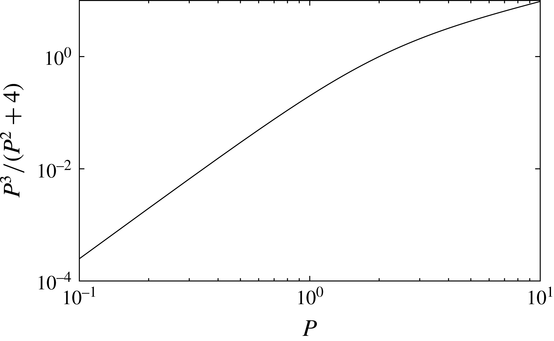
(by (4.25)), both the second and third terms of (5.12) are proportional to
 $P^{3}/(P^{2}+4)$
, depicted in figure 3. The velocity perturbation grows as
 $P^{3}$
for
 $P\ll 1$
, and then as
 $P$
for
 $P\gg 4$
. However, when
 $E_{0}$
and
 $P$
are sufficiently large the electro-neutrality condition (4.40) will no longer be satisfied, and the analysis fails.
The function
 $P^{3}/(P^{2}+4)\propto U_{1}$
.

The ratio of the second (positive) term in the velocity perturbation (5.12) to the linear (low field strength) electrophoretic velocity
 $U_{0}$
(3.17) is
 $$\begin{eqnarray}\displaystyle {\displaystyle \frac{5\unicode[STIX]{x1D716}(\unicode[STIX]{x1D701}_{c}+\unicode[STIX]{x1D701}_{s})E_{0}SP}{12\unicode[STIX]{x1D707}(P^{2}+4)U_{0}}}={\displaystyle \frac{(\unicode[STIX]{x1D701}_{s}+\unicode[STIX]{x1D701}_{c})^{2}}{(\unicode[STIX]{x1D701}_{s}-\unicode[STIX]{x1D701}_{c})}}(\unicode[STIX]{x1D70E}_{c}+\unicode[STIX]{x1D70E}_{s})(1+2\unicode[STIX]{x1D6FC}_{-}){\displaystyle \frac{5R^{2}\unicode[STIX]{x1D716}E_{0}^{2}\overline{f}\unicode[STIX]{x1D6FD}^{2}}{96(P^{2}+4)k^{2}T^{2}h_{0}^{3}n_{0}\unicode[STIX]{x1D707}}}. & & \displaystyle\end{eqnarray}$$
We now gather together the various constraints on the analysis. To ensure that the concentration of ions is approximately uniform across the gap between the two charge clouds on the cylinder and sphere, we require (4.24)
 $$\begin{eqnarray}\displaystyle P\ll {\displaystyle \frac{R}{h}}. & & \displaystyle\end{eqnarray}$$
To ensure that the number densities of co- and counter-ions within the gap are approximately equal (so that electro-neutrality holds at least to a first approximation), we require (4.40)
 $$\begin{eqnarray}\displaystyle {\displaystyle \frac{eE_{0}R}{\unicode[STIX]{x1D705}^{2}h_{0}\unicode[STIX]{x1D6FD}kT}}\ll 1. & & \displaystyle\end{eqnarray}$$
To ensure that the right-hand side of (4.30) may be treated as a small but non-negligible correction, we require, by (4.15)
 $$\begin{eqnarray}\displaystyle 1\ll \text{e}^{eZ\unicode[STIX]{x1D701}_{c}/kT}+\text{e}^{eZ\unicode[STIX]{x1D701}_{s}/kT}\ll h_{0}\unicode[STIX]{x1D705}. & & \displaystyle\end{eqnarray}$$
6 Concluding remarks
The leading-order expression (3.17) for the linear electrophoretic velocity
 $U_{0}$
when
 $h_{0}\ll R$
is zero if
 $\unicode[STIX]{x1D701}_{c}=\unicode[STIX]{x1D701}_{s}$
. A choice of identical materials for the sphere and cylinder will therefore facilitate the observation of electrophoretic velocities that are nonlinear in the applied field strength
 $E_{0}$
. When
 $\unicode[STIX]{x1D701}_{c}=\unicode[STIX]{x1D701}_{s}$
we expect the sphere to move forwards relative to the fluid at the same rate as the fluid moves backwards relative to the fixed wall of the cylinder. The net result is that an analysis linear in
 $E_{0}$
predicts that the sphere remains at rest and fluid is pumped backwards (relative to the laboratory frame) at both the cylindrical wall and at the surface of the sphere, assuming, of course, that fluid pumped electro-osmotically can enter at one end of the tube and leave at the other.
When the flux of counter-ions within the charge clouds is included in the ion conservation equations, the ionic density in the gap between the sphere and cylinder is reduced, leading to a net local increase in the slip velocities both at the cylindrical wall and at the sphere surface (at sufficiently high Péclet number
 $P$
). The increase in the slip velocity at the surface of the sphere tends to increase the electrophoretic velocity of the sphere relative to the fluid. The increase in slip velocity at the cylindrical wall, which pumps fluid backwards, is a local effect, and does not occur along the entire length of the cylinder. The only way for this locally enhanced backwards pumping to be accommodated is for the sphere to move forwards more rapidly, thereby making additional space for fluid behind it. Thus the changes in slip velocity at the two surfaces combine to enhance the change in electrophoretic velocity, rather than cancelling each other in the same manner as for identical zeta potentials and slip velocities at low field strengths.
Our aim has been to obtain the leading nonlinear
 $O(E^{3})$
contribution to the electrophoretic velocity, which is proportional to
 $S$
and is therefore small. However, in experiments it should be possible to distinguish
 $O(E^{3})$
contributions to the electrophoretic velocity from contributions linear in
 $E$
, whether these linear contributions come from the leading-order lubrication analysis (3.17), higher-order corrections to the linear lubrication analysis not considered here, or the linear correction terms in (5.11) that were neglected.
Our analysis assumes that the particle is on the axis of the cylinder. Symmetry arguments tell us that linear electrophoresis with a velocity proportional to the applied axial field strength must be parallel to the axis of the cylinder even when the particle lies off the axis. However, a spherical particle adjacent to a plane wall experiences an
 $O(\hat{E}_{0}^{2})$
force away from the wall when an electric field is applied parallel to the wall (Yariv Reference Yariv2006, Reference Yariv2016a
,Reference Yariv
b
), and this force decreases as the distance between the sphere and the wall increases. We therefore expect a slow drift of an off-axis particle towards the axis. This conclusion is supported by simple one-dimensional arguments that neglect azimuthal motion of ions and fluid when computing the perturbations
 $n_{1}$
and
 $\unicode[STIX]{x1D719}_{1}$
around an off-axis particle. Since
 $S\propto h_{0}^{-2}$
, the ionic concentration perturbation
 $n_{1}$
(4.28) will be more negative on the narrow side of the gap than on the wider side, and the perturbed potential
 $\unicode[STIX]{x1D719}_{1}$
(4.32) will be larger on the narrow side. The resulting azimuthal gradients of potential and concentration generate a fluid velocity (2.9) (relative to the particle) from the wide side of the gap to the narrow side, i.e. these gradients tend to move the particle towards the wide side and thus towards the centreline of the tube.
Acknowledgements
We thank our anonymous referees for suggestions that led to improvement of this paper. J.D.S. thanks the Department of Applied Mathematics and Theoretical Physics, University of Cambridge, for hospitality.
Appendix A. Fluid motion due to an external applied tangential electric field
We investigate fluid motion within a charge cloud adjacent to a plane charged surface, both in order to determine the slip velocity at the outer edge of the charge cloud, and to determine the convective flux of ions. Far from the charged surface, the ionic number density is
 $n_{\infty }=B^{2}n_{0}$
and the potential is
 $\unicode[STIX]{x1D719}_{\infty }$
. An electrical body force
 $-\unicode[STIX]{x1D70C}\unicode[STIX]{x1D735}\unicode[STIX]{x1D719}$
acts on the fluid, and the Stokes equation for motion normal to the boundary leads to the force balance
 $$\begin{eqnarray}\displaystyle {\displaystyle \frac{\unicode[STIX]{x2202}p}{\unicode[STIX]{x2202}y}}=eZn_{\infty }(\text{e}^{\hat{\unicode[STIX]{x1D711}}}-\text{e}^{-\hat{\unicode[STIX]{x1D711}}}){\displaystyle \frac{\unicode[STIX]{x2202}\unicode[STIX]{x1D713}}{\unicode[STIX]{x2202}y}}=kTn_{\infty }(\text{e}^{\hat{\unicode[STIX]{x1D711}}}-\text{e}^{-\hat{\unicode[STIX]{x1D711}}}){\displaystyle \frac{\unicode[STIX]{x2202}\hat{\unicode[STIX]{x1D711}}}{\unicode[STIX]{x2202}y}}, & & \displaystyle\end{eqnarray}$$
so that
 $$\begin{eqnarray}\displaystyle p=kTn_{\infty }(\text{e}^{\hat{\unicode[STIX]{x1D711}}}+\text{e}^{-\hat{\unicode[STIX]{x1D711}}}-2)+p_{\infty }=kT(n_{-}+n_{+}-2n_{\infty })+p_{\infty }, & & \displaystyle\end{eqnarray}$$
where the constant of integration is chosen such that
 $p_{\infty }$
is the fluid pressure outside the charge cloud,
 $p_{\infty }-2kTn_{\infty }$
the partial pressure due to the solvent outside the cloud and
 $kT(n_{-}+n_{+})$
is the van t’Hoff contribution to the osmotic pressure. The Stokes equation for the fluid velocity
 $\boldsymbol{u}$
tangential to the charged surface, within the double layer, is
 $$\begin{eqnarray}\displaystyle \unicode[STIX]{x1D707}{\displaystyle \frac{\unicode[STIX]{x2202}^{2}\boldsymbol{u}}{\unicode[STIX]{x2202}y^{2}}} & = & \displaystyle \unicode[STIX]{x1D735}_{t}p-eZn_{\infty }(\text{e}^{\hat{\unicode[STIX]{x1D711}}}-\text{e}^{-\hat{\unicode[STIX]{x1D711}}})\unicode[STIX]{x1D735}_{t}\unicode[STIX]{x1D713}\nonumber\\ \displaystyle & = & \displaystyle \unicode[STIX]{x1D735}_{t}p_{\infty }-eZn_{\infty }(\text{e}^{\hat{\unicode[STIX]{x1D711}}}-\text{e}^{-\hat{\unicode[STIX]{x1D711}}})\unicode[STIX]{x1D735}_{t}\unicode[STIX]{x1D719}_{\infty }+kT(\text{e}^{\hat{\unicode[STIX]{x1D711}}}+\text{e}^{-\hat{\unicode[STIX]{x1D711}}}-2)\unicode[STIX]{x1D735}_{t}n_{\infty }\nonumber\\ \displaystyle & = & \displaystyle \unicode[STIX]{x1D735}_{t}p_{\infty }-\frac{\unicode[STIX]{x1D716}kT}{eZ}{\displaystyle \frac{\unicode[STIX]{x2202}^{2}\hat{\unicode[STIX]{x1D711}}}{\unicode[STIX]{x2202}y^{2}}}\unicode[STIX]{x1D735}_{t}\unicode[STIX]{x1D719}_{\infty }+kT(\text{e}^{\hat{\unicode[STIX]{x1D711}}}+\text{e}^{-\hat{\unicode[STIX]{x1D711}}}-2)\unicode[STIX]{x1D735}_{t}n_{\infty }.\end{eqnarray}$$
We integrate (A 3) once:
 $$\begin{eqnarray}\displaystyle \unicode[STIX]{x1D707}{\displaystyle \frac{\unicode[STIX]{x2202}\boldsymbol{u}}{\unicode[STIX]{x2202}y}}=y\unicode[STIX]{x1D735}_{t}p_{\infty }-{\displaystyle \frac{\unicode[STIX]{x1D716}kT}{eZ}}{\displaystyle \frac{\unicode[STIX]{x2202}\hat{\unicode[STIX]{x1D711}}}{\unicode[STIX]{x2202}y}}\unicode[STIX]{x1D735}_{t}\unicode[STIX]{x1D719}_{\infty }-kT{\displaystyle \frac{4A}{B\unicode[STIX]{x1D705}}}\left[{\displaystyle \frac{1}{A-\text{e}^{-\unicode[STIX]{x1D702}B}}}+\frac{1}{A+\text{e}^{-\unicode[STIX]{x1D702}B}}\right]\unicode[STIX]{x1D735}_{t}n_{\infty }+\boldsymbol{C}, & & \displaystyle\end{eqnarray}$$
where
 $\boldsymbol{C}$
is a constant of integration. If the shear stress immediately outside the charge cloud (i.e. in the limit
 $\unicode[STIX]{x1D702}\rightarrow \infty$
) is
 $\unicode[STIX]{x1D707}\dot{\unicode[STIX]{x1D738}}_{w}$
, this determines
 $\boldsymbol{C}$
and we rewrite (A 4) as
 $$\begin{eqnarray}\displaystyle \unicode[STIX]{x1D707}{\displaystyle \frac{\unicode[STIX]{x2202}\boldsymbol{u}}{\unicode[STIX]{x2202}y}}=y\unicode[STIX]{x1D735}_{t}p_{\infty }-{\displaystyle \frac{\unicode[STIX]{x1D716}kT}{eZ}}\frac{\unicode[STIX]{x2202}\hat{\unicode[STIX]{x1D711}}}{\unicode[STIX]{x2202}y}\unicode[STIX]{x1D735}_{t}\unicode[STIX]{x1D719}_{\infty }-kT\frac{4}{B\unicode[STIX]{x1D705}}\left[\frac{\text{e}^{-\unicode[STIX]{x1D702}B}}{A-\text{e}^{-\unicode[STIX]{x1D702}B}}-{\displaystyle \frac{\text{e}^{-\unicode[STIX]{x1D702}B}}{A+\text{e}^{-\unicode[STIX]{x1D702}B}}}\right]\unicode[STIX]{x1D735}_{t}n_{\infty }+\unicode[STIX]{x1D707}\dot{\unicode[STIX]{x1D738}}_{w}. & & \displaystyle\end{eqnarray}$$
A second integration gives
 $$\begin{eqnarray}\displaystyle \unicode[STIX]{x1D707}\boldsymbol{u} & = & \displaystyle {\displaystyle \frac{y^{2}}{2}}\unicode[STIX]{x1D735}_{t}p_{\infty }+\unicode[STIX]{x1D707}\dot{\unicode[STIX]{x1D738}}_{w}y-\frac{\unicode[STIX]{x1D716}kT}{eZ}\hat{\unicode[STIX]{x1D711}}\unicode[STIX]{x1D735}_{t}\unicode[STIX]{x1D719}_{\infty }\nonumber\\ \displaystyle & & \displaystyle -\,\frac{4kT}{B^{2}\unicode[STIX]{x1D705}^{2}}\left[\ln (A-\text{e}^{-\unicode[STIX]{x1D702}B})+\ln (A+\text{e}^{-\unicode[STIX]{x1D702}B})\right]\unicode[STIX]{x1D735}_{t}n_{\infty }+\boldsymbol{C}_{2},\end{eqnarray}$$
where the constant of integration
 $\boldsymbol{C}_{2}$
is chosen in order to satisfy the no-slip boundary condition on the surface
 $y=0$
, and hence
 $$\begin{eqnarray}\displaystyle \unicode[STIX]{x1D707}\boldsymbol{u} & = & \displaystyle \frac{y^{2}}{2}\unicode[STIX]{x1D735}_{t}p_{\infty }+\unicode[STIX]{x1D707}\dot{\unicode[STIX]{x1D738}}_{w}y-\unicode[STIX]{x1D716}(\unicode[STIX]{x1D713}-\unicode[STIX]{x1D719}_{\infty }-\unicode[STIX]{x1D701})\unicode[STIX]{x1D735}_{t}\unicode[STIX]{x1D719}_{\infty }\nonumber\\ \displaystyle & & \displaystyle -\,\frac{4kT}{B^{2}\unicode[STIX]{x1D705}^{2}}\left[\ln \left(\frac{A-\text{e}^{-\unicode[STIX]{x1D702}B}}{A-1}\right)+\ln \left(\frac{A+\text{e}^{-\unicode[STIX]{x1D702}B}}{A+1}\right)\right]\unicode[STIX]{x1D735}_{t}n_{\infty }.\end{eqnarray}$$
The slip velocity
 $u_{slip}$
just outside the charge cloud is obtained by taking the limit
 $\unicode[STIX]{x1D702}\rightarrow \infty$
(so that
 $\unicode[STIX]{x1D713}\rightarrow \unicode[STIX]{x1D719}_{\infty }$
) while ignoring the terms due to the external pressure gradient
 $\unicode[STIX]{x1D735}_{t}p_{\infty }$
and shear stress
 $\unicode[STIX]{x1D707}\dot{\unicode[STIX]{x1D738}}_{w}y$
. We find
 $$\begin{eqnarray}\displaystyle \boldsymbol{u}_{slip} & = & \displaystyle \frac{\unicode[STIX]{x1D716}\unicode[STIX]{x1D701}}{\unicode[STIX]{x1D707}}\unicode[STIX]{x1D735}_{t}\unicode[STIX]{x1D719}_{\infty }-\frac{4kT}{\unicode[STIX]{x1D707}B^{2}\unicode[STIX]{x1D705}^{2}}\ln \left(\frac{A^{2}}{A^{2}-1}\right)\unicode[STIX]{x1D735}_{t}n_{\infty }\nonumber\\ \displaystyle & = & \displaystyle \frac{\unicode[STIX]{x1D716}\unicode[STIX]{x1D701}}{\unicode[STIX]{x1D707}}\unicode[STIX]{x1D735}_{t}\unicode[STIX]{x1D719}_{\infty }-\frac{4\unicode[STIX]{x1D716}(kT)^{2}}{\unicode[STIX]{x1D707}e^{2}Z^{2}}\ln [\cosh (\hat{\unicode[STIX]{x1D701}}/4)]\unicode[STIX]{x1D735}_{t}\ln n_{\infty }.\end{eqnarray}$$
If we take the limit
 $Ze\unicode[STIX]{x1D701}/kT\gg 1$
, this slip velocity can be written as
 $$\begin{eqnarray}\displaystyle \boldsymbol{u}_{slip}\approx \frac{\unicode[STIX]{x1D716}\unicode[STIX]{x1D701}}{\unicode[STIX]{x1D707}eZ}\unicode[STIX]{x1D735}_{t}\left(Ze\unicode[STIX]{x1D719}_{\infty }-kT\ln n_{\infty }\right), & & \displaystyle\end{eqnarray}$$
proportional to the gradient of the electrochemical potential of the negative counter-ions outside the charge cloud.
Appendix B. Tangential ionic fluxes within a double layer
A tangential electric field or concentration gradient applied outside a charge cloud creates fluxes of ions within the cloud. These fluxes are small if the number of ions within the cloud is small, but lead to a non-negligible surface current if many ions are present (as occurs if the charge density on the charged surface is sufficiently high). These currents, discussed by O’Brien (Reference O’Brien1983), have been studied by Schnitzer & Yariv (Reference Schnitzer and Yariv2012b ) who use matched asymptotic expansions to treat the different portions of the charge cloud. We present an analysis along the lines adopted by Hinch et al. (Reference Hinch, Sherwood, Chew and Sen1984), extended to include the effect of concentration gradients.
The radial ionic flux balance tells us that to leading order the ionic number density of the
 $i$
th ionic species within the charge cloud satisfies a Maxwell–Boltzmann distribution of the form
 $$\begin{eqnarray}\displaystyle n_{i}=n_{\infty }\exp (-Z_{i}e(\unicode[STIX]{x1D713}-\unicode[STIX]{x1D719}_{\infty })/kT), & & \displaystyle\end{eqnarray}$$
where
 $n_{\infty }$
is the number density of ions just outside the charge cloud, and
 $\unicode[STIX]{x1D719}_{\infty }$
is the electrical potential just outside the cloud. We know from previous work (Hinch et al.
Reference Hinch, Sherwood, Chew and Sen1984; Schnitzer & Yariv Reference Schnitzer and Yariv2014) that the ionic number density may be perturbed away from the number density
 $n_{0}$
in the bulk electrolyte solution, but that charge densities will be small (though not zero, as discussed by Schnitzer & Yariv (Reference Schnitzer and Yariv2014)), so that the prefactor
 $n_{\infty }$
in (B 1) is the same for both ionic species.
The electrochemical potential of the ions does not vary rapidly across the thin double layer, so tangential fluxes of ions driven by gradients of electrochemical potential may be evaluated using the tangential gradient of electrochemical potential
 $-\unicode[STIX]{x1D735}_{t}[kT\ln (n_{\infty })+eZ_{i}\unicode[STIX]{x1D719}_{\infty }]$
. The excess flux due to the presence of the double layer is
 $$\begin{eqnarray}\displaystyle \boldsymbol{F}_{1i}=-\unicode[STIX]{x1D714}_{i}\int (n_{i}-n_{\infty })\unicode[STIX]{x1D735}_{t}[kT\ln (n_{\infty })+eZ_{i}\unicode[STIX]{x1D719}_{\infty }]\,\text{d}y, & & \displaystyle\end{eqnarray}$$
where the integration is across the thickness of the charge cloud. Substituting the ionic number density (B 1) into (B 2) gives the flux
 $$\begin{eqnarray}\displaystyle \boldsymbol{F}_{1i}=-\unicode[STIX]{x1D714}_{i}\int \left\{\left[\exp \left(-\frac{Z_{i}e(\unicode[STIX]{x1D713}-\unicode[STIX]{x1D719}_{\infty })}{kT}\right)-1\right][kT\unicode[STIX]{x1D735}_{t}n_{\infty }+n_{\infty }eZ_{i}\unicode[STIX]{x1D735}_{t}\unicode[STIX]{x1D719}_{\infty }]\right\}\,\text{d}y. & & \displaystyle\end{eqnarray}$$
For the positive co-ions, this is
 $$\begin{eqnarray}\displaystyle \boldsymbol{F}_{1+} & = & \displaystyle \unicode[STIX]{x1D714}_{+}[kT\unicode[STIX]{x1D735}_{t}n_{\infty }+n_{\infty }eZ\unicode[STIX]{x1D735}_{t}\unicode[STIX]{x1D719}_{\infty }]\int _{0}^{\infty }\frac{4A\text{e}^{-\unicode[STIX]{x1D702}B}}{(A+\text{e}^{-\unicode[STIX]{x1D702}B})^{2}}\frac{\text{d}\unicode[STIX]{x1D702}}{\unicode[STIX]{x1D705}}\nonumber\\ \displaystyle & = & \displaystyle \frac{4\unicode[STIX]{x1D714}_{+}}{\unicode[STIX]{x1D705}B(A+1)}[kT\unicode[STIX]{x1D735}_{t}n_{\infty }+n_{\infty }eZ\unicode[STIX]{x1D735}_{t}\unicode[STIX]{x1D719}_{\infty }].\end{eqnarray}$$
Since
 $\unicode[STIX]{x1D705}^{-1}$
is small compared to length scales tangential to the surface, this flux is small. For the negative counter-ions, the contribution to the flux is
 $$\begin{eqnarray}\displaystyle \boldsymbol{F}_{1-} & = & \displaystyle -\unicode[STIX]{x1D714}_{-}[kT\unicode[STIX]{x1D735}_{t}n_{\infty }-n_{\infty }eZ\unicode[STIX]{x1D735}_{t}\unicode[STIX]{x1D719}_{\infty }]\int _{0}^{\infty }\frac{4A\text{e}^{-\unicode[STIX]{x1D702}B}}{(A-\text{e}^{-\unicode[STIX]{x1D702}B})^{2}}\frac{\text{d}\unicode[STIX]{x1D702}}{\unicode[STIX]{x1D705}}\nonumber\\ \displaystyle & = & \displaystyle -\frac{4\unicode[STIX]{x1D714}_{-}}{\unicode[STIX]{x1D705}B}\frac{(\text{e}^{\hat{\unicode[STIX]{x1D701}}/2}-1)}{2}[kT\unicode[STIX]{x1D735}_{t}n_{\infty }-n_{\infty }eZ\unicode[STIX]{x1D735}_{t}\unicode[STIX]{x1D719}_{\infty }].\end{eqnarray}$$
Since
 $\unicode[STIX]{x1D705}^{-1}$
is small, this flux is small unless
 $\text{e}^{\hat{\unicode[STIX]{x1D701}}/2}$
is large, in which case this contribution to the flux of counter-ions cannot be neglected.
We now consider the additional convection of ions within the charge cloud, i.e. we evaluate
 $$\begin{eqnarray}\displaystyle \boldsymbol{F}_{2i}=\int \boldsymbol{u}(n_{i}-n_{\infty })\,\text{d}y, & & \displaystyle\end{eqnarray}$$
where the integral, as in (B 2), is across the thickness of the charge cloud, and the tangential fluid velocity
 $\boldsymbol{u}$
is given by (A 7). We neglect the (small) contributions due to the externally imposed pressure gradient and shear rate, and consider only contributions due to the gradients in electrochemical potential. For the positive co-ions, we find
 $$\begin{eqnarray}\displaystyle \boldsymbol{F}_{2+} & = & \displaystyle n_{\infty }\int \boldsymbol{u}(\text{e}^{-\hat{\unicode[STIX]{x1D711}}}-1)\,\text{d}y\nonumber\\ \displaystyle & = & \displaystyle -\frac{\unicode[STIX]{x1D716}kT}{\unicode[STIX]{x1D707}eZ}\frac{8n_{\infty }}{\unicode[STIX]{x1D705}B}\left[\frac{1}{A+1}+\frac{1}{2}\ln \left(\frac{A-1}{A+1}\right)\right]\unicode[STIX]{x1D735}_{t}\unicode[STIX]{x1D719}_{\infty }\nonumber\\ \displaystyle & & \displaystyle -\,\frac{4kT}{\unicode[STIX]{x1D707}B^{2}\unicode[STIX]{x1D705}^{2}}\frac{4n_{\infty }}{B\unicode[STIX]{x1D705}}\left[\frac{1}{2}\ln \left(\frac{A^{2}}{A^{2}-1}\right)+\ln \left(\frac{A}{A+1}\right)+\frac{1}{A+1}\right]\unicode[STIX]{x1D735}_{t}n_{\infty }.\end{eqnarray}$$
For the negative counter-ions, the convective flux is
 $$\begin{eqnarray}\displaystyle \boldsymbol{F}_{2-} & = & \displaystyle n_{\infty }\int \boldsymbol{u}(\text{e}^{\hat{\unicode[STIX]{x1D711}}}-1)\,\text{d}y\nonumber\\ \displaystyle & = & \displaystyle -\frac{\unicode[STIX]{x1D716}kT}{\unicode[STIX]{x1D707}eZ}\frac{8n_{\infty }}{\unicode[STIX]{x1D705}B}\left[-\frac{1}{A-1}+\frac{1}{2}\ln \left(\frac{A+1}{A-1}\right)\right]\unicode[STIX]{x1D735}_{t}\unicode[STIX]{x1D719}_{\infty }\nonumber\\ \displaystyle & & \displaystyle -\,\frac{4kT}{\unicode[STIX]{x1D707}B^{2}\unicode[STIX]{x1D705}^{2}}\frac{4n_{\infty }}{B\unicode[STIX]{x1D705}}\left[-\ln \left(\frac{A}{A-1}\right)+\frac{1}{A-1}-\frac{1}{2}\ln \left(\frac{A^{2}}{A^{2}-1}\right)\right]\unicode[STIX]{x1D735}_{t}n_{\infty }.\end{eqnarray}$$
The total excess tangential flux of ions within the charge cloud is the sum of the flux
 $\boldsymbol{F}_{1}$
generated by the gradient of chemical potential, and the convective flux
 $\boldsymbol{F}_{2}$
. These fluxes are large only for the negative counter-ions, and the largest terms in (B 5) and (B 8) are
 $$\begin{eqnarray}\displaystyle \boldsymbol{F}_{1-}+\boldsymbol{F}_{2-}\sim \frac{4}{\unicode[STIX]{x1D705}B(A-1)}\left(\unicode[STIX]{x1D714}_{-}+\frac{2kT\unicode[STIX]{x1D716}}{\unicode[STIX]{x1D707}e^{2}Z^{2}}\right)\left[kT\unicode[STIX]{x1D735}_{t}n_{\infty }-n_{\infty }eZ\unicode[STIX]{x1D735}_{t}\unicode[STIX]{x1D719}_{\infty }\right]. & & \displaystyle\end{eqnarray}$$
When
 $Ze\unicode[STIX]{x1D701}/kT\gg 1$
, so that
 $A\approx 1+2\text{e}^{-\hat{\unicode[STIX]{x1D701}}/2}$
, then
 $$\begin{eqnarray}\displaystyle {\displaystyle \frac{1}{A-1}}\approx {\displaystyle \frac{\text{e}^{\hat{\unicode[STIX]{x1D701}}/2}}{2}}\approx \frac{Ze\unicode[STIX]{x1D70E}}{2\unicode[STIX]{x1D716}\unicode[STIX]{x1D705}BkT}. & & \displaystyle\end{eqnarray}$$
Hence, when the zeta potential is large, the excess tangential flux of counter-ions can be expressed in the form
 $$\begin{eqnarray}\displaystyle \boldsymbol{F}_{1-}+\boldsymbol{F}_{2-}\approx -{\displaystyle \frac{\unicode[STIX]{x1D70E}\unicode[STIX]{x1D714}_{-}}{eZ}}(1+2\unicode[STIX]{x1D6FC}_{-})\unicode[STIX]{x1D735}_{t}[kT\ln (n_{\infty })-eZ\unicode[STIX]{x1D719}_{\infty }], & & \displaystyle\end{eqnarray}$$
where, using the notation of Schnitzer & Yariv (Reference Schnitzer and Yariv2014),
 $$\begin{eqnarray}\displaystyle \unicode[STIX]{x1D6FC}_{-}={\displaystyle \frac{\unicode[STIX]{x1D716}kT}{Z^{2}e^{2}\unicode[STIX]{x1D707}\unicode[STIX]{x1D714}_{-}}}. & & \displaystyle\end{eqnarray}$$