1.0 INTRODUCTION
The use of fibre-reinforced composites in aerospace and marine structures has become widespread due to their high stiffness-to-weight and strength-to-weight ratios. Designs of laminate configurations of composite panels, including laminate thicknesses and stacking sequences, are of vital importance to achieve the required structure mechanical behaviour for specific sets of loading conditions.
There are three main types of widely researched(Reference Ghiasi, Pasini and Lessard1) optimisation methods for composite structures:
(1) The smeared stiffness-based method ( Reference Schmit and Mehrinfar 2 - Reference Liu, Toropov, Querin and Barton 4 ) is commonly used in industry: –45/0/45/90 thickness percentages are used as design variables to carry out the optimisation, and the mathematical programming method and optimality criteria method are always used. This smeared stiffness-based method approximates the bending stiffness matrix via the homogeneous laminate assumption, that is, D = h2/12×A (with D and A referring to the D and A matrix of composite laminate), but the influence of the stacking sequence is weakened and the global optimum cannot be guaranteed.
(2) For laminate design, the layer thickness for each material is usually fixed and fibre orientation angles are often limited to discrete sets such as 0°, ±45° and 90° due to manufacturing constraints. The discrete nature of the design problem leads to the development of powerful genetic algorithms or GAs (and other evolution algorithms) for composite stacking sequence optimisation(Reference Riche and Haftka5 - Reference Todoroki and Haftka9). Sivakumar(Reference Sivakumar, Iyengar and Deb7) concluded that 'GA seems to be the best tool to optimise composite laminates'. However, genetic algorithms are well known for being expensive optimisation tools, especially if the cost for analysis of each individual design is high.
(3) Instead of layer angles and layer thicknesses, lamination parameters seem to be more reliable design variables because the laminate stiffness matrices are linear in terms of the lamination parameters, so several design problems can be formulated as convex optimisation problems using lamination parameters(Reference Diaconu and Sekine10 - Reference Setoodeh, Abdalla and Gürdal13). One of the limitations and perhaps objections to using lamination parameters for composite design has been the difficulty of incorporating ply-level strength constraints into the optimisation process(Reference IJsselmuiden14).
Lamination parameters were firstly used by Tsai et al(Reference Tsai and Hahn15). Miki(Reference Miki and Sugiyama16) and Fukunaga(Reference Fukunaga and Vanderplaats17) used the lamination parameters method for tailoring mechanical properties of laminated composites and analysed the feasible region of lamination parameters. Diaconu et al( Reference Diaconu and Sekine 10 , Reference Diaconu, Sato and Sekine 18 ) used a variational approach to determine feasible regions in the space of lamination parameters as constraints in the optimisation problem. When limiting plies to a fixed set of angles, the feasible region in LP space is known(Reference Bloomfield, Diaconu and Weaver19). The idea of looking for a laminate with lamination parameters closest to the continuous solution has been suggested by Yamazaki(Reference Yamazaki20). Todoroki et al(Reference Todoroki and Sasai21) made use of a global response surface, while Herencia et al(Reference Herencia, Haftka, Weaver and Friswell22) constructed a linear approximation of the design constraints around the optimum continuous design to achieve the better laminates’ stacking sequences in the design space. Recently, many researchers have been devoted to development of the lamination parameters method( Reference Liu, Toropov, Barton and Querin 23 - Reference Bohrer, Almeida and Donadon 26 ).
For large composite wings, the optimisation panel is often divided into several smaller sub-regions to improve structure performance with weight reduction. A common problem with the design of composite structures is that the laminate configurations between adjacent regions may vary from each other (i.e. different thickness and stacking sequence exist), causing incompatibilities in the stacking sequence(Reference Yamazaki20). These incompatibilities will increase manufacturing difficulties and costs for structure integrity design. Thus, stacking sequence compatibility design of laminate panels has been gaining more and more attention.
Since the term blending has been introduced by Kristinsdottir et al to illustrate the continuity problem(Reference Kristinsdottir, Zabinsky, Tuttle and Neogi27), many researchers have been studying the composite structure blending models. Liu(Reference Liu and Haftka28) and Toropov(Reference Toropov, Jones and Willment29) imposed measures of material composition continuity and stacking sequence continuity between two adjacent panels to get a blended composite panel. Soremekun et al(Reference Soremekun, Gürdal, Kassapoglou and Toni30) used multiple sub-laminates and a design variable zone approach to design completely blended composite structures. Adams(Reference Adams, Watson, Gürdal and Anderson-Cook31) and Seresta(Reference Seresta, Abdalla and Gürdal32) achieved a blended solution using a guide-based genetic algorithm and developed two blending models, inner and outer blending, to improve the ply continuity between adjacent laminates. Campen(Reference Campen, Seresta and Abdalla33) proposed two new blending definitions, generalised blending and relaxed generalised blending. Irisarri(Reference Irisarri, Lasseigne, Leroy and Riche34) introduced a concept of stacking sequence table (SST) for the optimal design of laminated composite structures with ply drops, while Zein( Reference Zein, Basso and Grihon 35 , Reference Zein, Basso and Grihon 36 ) proposed a primal-dual backtracking optimisation method for finding the optimal stacking sequence and the ply drop-offs of a blended composite structure. Jing( Reference Jing, Fan and Sun 37 , Reference Jing, Fan and Sun 38 ) proposed a Global Shared-Layer Blending (GSLB) method for obtaining a manufacturable stacking sequence of composite structures with blending and design rules. Yang(Reference Yang, Song, Zhong and Jin39) studied an optimal design method of blended composite laminate structures using a ply drop sequence.
For blending design of composite panels with lamination parameters, Liu(Reference Liu, Toropov, Querin and Barton4) chose the lamination parameters and numbers of plies as design variables in the first level to minimise the material volume, and the Shared Layers Blending (SLB) method is used to get an optimal stacking sequence with manufacturing requirements. IJsselmuiden(Reference IJsselmuiden, Abdalla, Seresta and Gürdal40) presented a two-step composite design framework using lamination parameters as design variables in the first level, and produced fully blended designs incorporating a guide based genetic algorithm in the second level. The multi-step approach is efficient for the eighteen panel horseshoe configuration composite structure with buckling constraints. However, if multiple types of structure behaviour constraints are considered, the multi-step approach may produce some problems. For example, the laminate strength constraints cannot be considered well. Strength constraints based on popular failure criteria such as the Tsai–Wu criterion depend not only on the stiffness properties, but also explicitly on ply angles. A conservative failure envelope is derived that guarantees a failure-free region of the lamination parameter space regardless of the fibre orientations in the laminate stacking sequence by IJsselmuiden(Reference IJsselmuiden, Abdalla and Gürdal44). The derived envelope is shown to accurately represent the safety factor of practical laminates under in-plane loading; however, for bending dominated problems, it may be too conservative(Reference IJsselmuiden, Abdalla and Gürdal44).
In the present study, on the basis of the guide-based blending model, a new optimisation method incorporating the lamination parameters is proposed. Instead of using lamination parameters of each panel as design variables as in IJsselmuidenReference IJsselmuiden, Abdalla, Seresta and Gürdal 40 does, lamination parameters of a guide laminate and the number of plies for each panel are used as design variables for optimisation. A parallel genetic algorithm(Reference Jin, Song and Zhong41,Reference Erick45) is used to get the global optimum with structure behaviour constraints and manufacturing constraints. In order to obtain the laminate configuration of each panel for each individual during the optimisation process, another genetic algorithm is used for each individual: firstly, with a form of least squares fitting adopted, the guide stacking sequence is obtained from the guide lamination parameters values; secondly, the laminate configurations of each panel are calculated from the optimum guide stacking sequence and ply number of each panel for structure analysis. Two genetic algorithms are used in this method, one for the optimisation process and the other for solving the real guide stacking sequence.
2.0 OPTIMISATION METHODOLOGY
2.1 Lamination parameters
According to Classical Laminate Theory (CLT)(Reference Jones42), the membrane, coupling and bending lamination parameters are given, respectively, by the following integrals:
 $$\begin{equation}
V_{[1\;\;2\;\;3\;\;4]}^{\rm{A}} = \frac{1}{h}\int_{ - h/2}^{h/2} {[\cos 2\theta \;\;\cos 4\theta \;\;\sin 2\theta \;\;\sin 4\theta ]} dz,
\end{equation}$$
 $$\begin{equation}
V_{[1\;\;2\;\;3\;\;4]}^{\rm{B}} = \frac{4}{{{h^2}}}\int_{ - h/2}^{h/2} {[\cos 2\theta \;\;\cos 4\theta \;\;\sin 2\theta \;\;\sin 4\theta ]z} dz,
\end{equation}$$
 $$\begin{equation}
V_{[1\;\;2\;\;3\;\;4]}^{\rm{D}} = \frac{{12}}{{{h^3}}}\int_{ - h/2}^{h/2} {[\cos 2\theta \;\;\cos 4\theta \;\;\sin 2\theta \;\;\sin 4\theta ]{z^2}} dz
\end{equation}$$
For symmetric laminates, the number of non-zero independent lamination parameters can be reduced to eight, and for symmetric laminates with 0°, 90°, 45°, and –45° fibre angles, the number of non-zero lamination parameters is further reduced to six.
2.2 Guide-based blending model
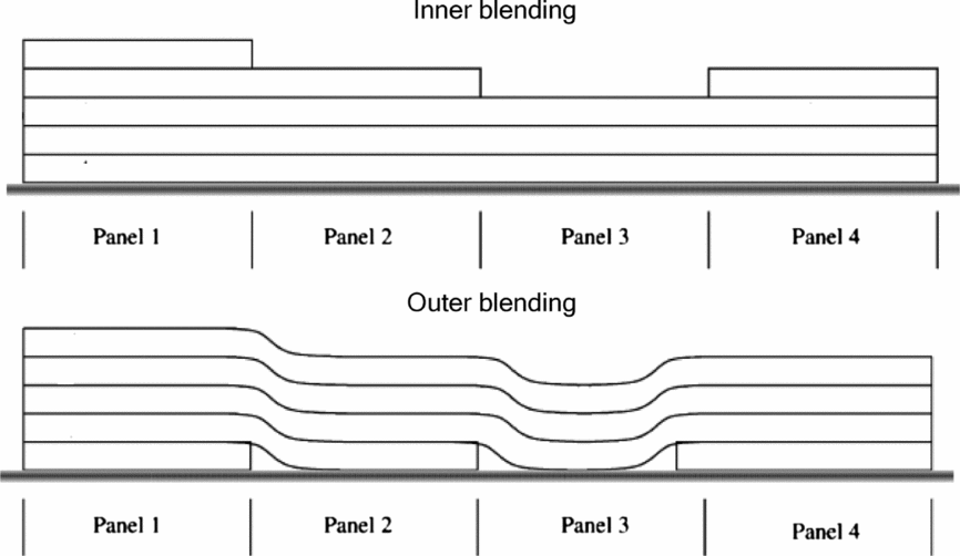
In the guide-based design (see Fig. 1), the basic laminate stacking sequence (referred as the guide) that is applicable to all the panels is used as a design layup, while the individual local panels use only a segment of the guide starting either from the top or from the bottom of the guide. This ensures complete blending at any stage of the design optimisation process. According to Adams et al(Reference Adams, Watson, Gürdal and Anderson-Cook31), for inner and outer blending models, the design variables are the stacking sequence of the guide defined by a vector θ of ply angles and the number of plies to be kept for each panel ni , where i is the number of panels. The corresponding encoded chromosomes for ply angles are 1, 2, 3 and 4 for 0°, 45°, –45° and 90°, respectively.
Inner and outer blending model.

For example, string [1243|421] demonstrates the individual includes three panels, the string [1243] represents the guide laminate configuration of (0/45/90/–45). For inner blending, the string [421] represents laminate configurations of the three panels of (0/45/90/–45), (90/–45), (–45), respectively.
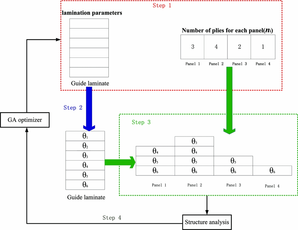
2.3 Optimisation procedure step
For structures consisting of multiple panels, the optimisation methodology process based on lamination parameters and blending models is as follows:
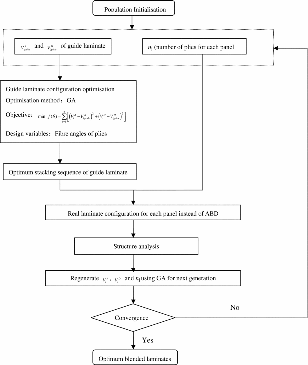
Step 1: set the number of plies for a guide laminate, initialise the population with lamination parameters of guide laminate (VA iguide and VD iguide , i = 1, 2, 3), and number of plies for each panel (n j, j = 1, 2. . .N, N denoting number of panels) as design variables.
Step 2: with a form of least squares fitting (Equation 4) as objective and fibre angles of plies as design variables for the guide laminate, a genetic algorithm is used for the inverse problem to decide the stacking sequence (θ 1/θ 2/θ 3/θ 4/. . .)s of the guide laminate to target the lamination parameters of the guide laminate.
 $$\begin{equation}
\min {\rm{ }}f(\theta ) = \sum\limits_{i = 1}^3 {\left[ {{{\left( {V_i^A - V_{iguide}^A} \right)}^2} + {{\left( {V_i^D - V_{iguide}^D} \right)}^2}} \right]}
\end{equation}$$
where VA iguide , VD iguide (i = 1, 2, 3) are the guide lamination parameters defined in Step 1, and VA i , VD i (i = 1, 2, 3) denote the lamination parameters calculated from the real laminate configuration.
Step 3: the laminate configurations of each panel are obtained based on the stacking sequence of the guide laminate (θ 1/θ 2/θ 3/θ 4/. . .)s and ply number of each panel (n j) for structure analysis.
Step 4: the lamination parameters of guide laminate and ply number of each panel are adjusted using GA with structure behaviour constraints (a strength constraint, stiffness constraint, buckling constraint, etc.) and manufacturing constraints (the four-contiguous ply rule, etc.) to generate the next population. Then go to Step 2.
The optimisation process is outlined graphically in Figs 2 and 3.
The four-step optimisation process.

Optimisation process flowchart.

Compared to the guide-based blending genetic algorithm, the number of design variables of the method proposed is smaller, leading to the possibility of smaller population sizes and generation cycles for the genetic algorithm to reduce the optimisation time. If the calculation time of the inverse problem to get the optimum laminate configuration is smaller than structure analysis time, the method will be more efficient, especially for aeroelastic tailoring problems. Moreover, real laminate configurations of the panels are used for structure analysis instead of lamination parameters, so any FE solver can be use with laminated shells instead of specifying the ABD directly compared with conventional lamination parameter method. Therefore, not only the global response constraints but also the local response constraints can be applied. The difficulty of incorporating strength constraints (Tsai-Wu strength criteria, etc.) into the optimisation process has been solved with this method.
3.0 REAL-CODED MASTER-SLAVE PARALLEL GENETIC ALGORITHM
Lamination parameters are real parameters with a range from –1 to +1. Since it is natural to choose the floating-point representation of genes of individuals, real-coded genetic algorithm is adopted to the optimisation problems in this paper. The GA used in this paper consists of the following steps:
3.1 Population initialisation
Lamination parameters are real parameters with a range from –1 to +1 continuous design variable. Since it is natural to choose the floating-point representation of genes of individuals, a real-coded genetic algorithm is adopted to the optimisation problems in this paper. The thicknesses of the face sheets and the core are decoded as real-coded strings.
The modelling of the genes for composite structure is as follows: (VA 1guide , VA 2guide , VA 3guide , VD 1guide , VD 2guide , VD 3guide , n 1, n 2,. . .n j,. . .n N). VA iguide and VD iguide are lamination parameters of the guide laminate, n j is the number of plies for each panel. N denotes number of panels.
3.2 GA crossover operation
Simulated binary crossover operator proposed by Deb are used for a real-coded genetic algorithm(Reference Deb and Agrawal43). We assume that two parents x (1) and x (2) are selected and crossed with a crossover probability P c. The chromosomes are crossed variable by variable to created two new children y (1) and y (2). Each variable (gene) is crossed with a probability of 0.5 using the following procedure:
Step 1: Create a random number μ ∈ [0, 1].
Step 2: Calculate βq as follows:
 $$\begin{equation}
{\beta _{\rm{q}}} = \left\{ \begin{array}{l} {(\alpha \mu )^{\frac{1}{{{\eta _c} + 1}}}}\quad\,{\it if}\,\mu \le {\alpha ^{ - 1}}\\ {\left( {\frac{1}{{2 - \alpha \mu }}} \right)^{\frac{1}{{{\eta _c} + 1}}}}\quad{\it otherwise} \end{array} \right.,
\end{equation}$$
where α = 2 − β− (ηc + 1), and β is calculated as follows
 $$\begin{equation}
\beta = \left\{ {\begin{array}{*{20}{c}} {1 + \frac{2}{{x_i^{(2)} - x_i^{(1)}}}\min \left[ {x_i^{(1)} - {x_i}^L,{x_i}^U - x_i^{(2)}} \right],\quad{\rm{ if }}x_i^{(1)} < x_i^{(2)}}\\[8pt] {1 + \frac{2}{{x_i^{(1)} - x_i^{(2)}}}\min \left[ {x_i^{(2)} - {x_i}^L,{x_i}^U - x_i^{(1)}} \right],\quad{\rm{ if }}x_i^{(2)} > x_i^{(1)}} \end{array}} \right.,
\end{equation}$$
where xL i and xU i are lower and upper bounds of variable xi , respectively. The user-defined parameter ηcis the distribution index. In all simulations, we set ηc = 15.
Step 3: the children are then computed as follows
 $$\begin{equation}
\begin{array}{l} y_i^{(1)} = 0.5\left[ {\left( {x_i^{(1)} + x_i^{(2)}} \right) - {\beta _q}\left| {x_i^{(2)} - x_i^{(1)}} \right|} \right]\\[8pt] y_i^{(2)} = 0.5\left[ {\left( {x_i^{(1)} + x_i^{(2)}} \right) + {\beta _q}\left| {x_i^{(2)} - x_i^{(1)}} \right|} \right] \end{array}
\end{equation}$$
3.3 GA mutation operation
A polynomial probability distribution(Reference Irisarri, Lasseigne, Leroy and Riche34) is performed to create a new chromosome y in the vicinity of a parent chromosome x. The operator is used for each variable with a probability of 0.1 in the following procedure:
Step 1: Create a random number μ ∈ [0, 1].
Step 2: Calculate δq as follows:
 $$\begin{equation}
{\delta _q} = \left\{ \begin{array}{l} - 1 + {\left[ {2\mu + (1 - 2\mu ){{(1 - \delta )}^{{\eta _{\rm{m}}} + 1}}} \right]^{\frac{1}{{{\eta _{\rm{m}}} + 1}}}}\quad{\rm{if}}\,\mu \le 0.5\\[4pt] 1 - {\left[ {2\left( {1{\rm{ - }}\mu } \right){\rm{ + }}2\left( {\mu - 0.5} \right){{\left( {1 - \delta } \right)}^{{\eta _{\rm{m}}} + 1}}} \right]^{\frac{1}{{{\eta _m} + 1}}}}\quad{\rm{otherwise}} \end{array} \right.,
\end{equation}$$
where
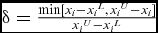 $\delta = \frac{{\min [ {{x_i} - {x_i}^L,{x_i}^U - {x_i}} ]}}{{{x_i}^U - {x_i}^L}}$
, and η
m
is the distribution index for mutation, we use η
m
= 20 here.
Step 3: Calculate the mutated child as follows:
 $$\begin{equation}
{y_i} = {x_i} + {\delta _q}\left( {x_i^U - x_i^L} \right)
\end{equation}$$
3.4 Elitist selection
The tournament selection method is chosen. When the two individuals both satisfy constraints, the one with lower object is the better; when just one of the individuals satisfies constraints, the one satisfying constraints is the better one; when neither of the two individuals satisfies constraints, the one with lower violation grade is the better one. The characteristic of tournament GA is that the individual with better fitness has greater opportunity. It can avoid the influence of a super-individual while controlling selection pressure and balancing evolution speed to overcome prematurity and stagnancy.
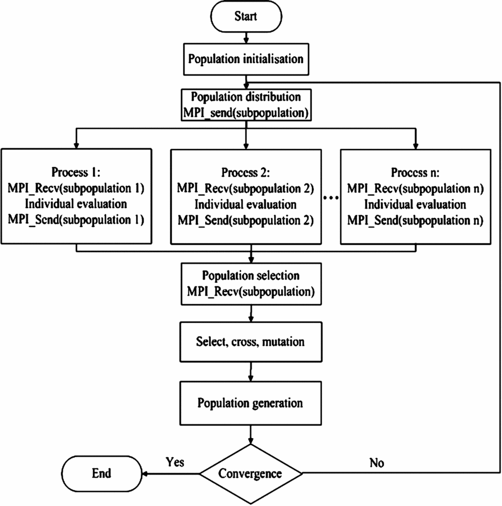
To decrease optimisation time, we use a parallel genetic algorithm that has three types: master-slave parallel GA, coarse-grain GA and fine-grain GA. The master-slave GA system is divided into one master process and several slave processes(Reference Erick45). The master process controls the whole population and carries on the operation of selection, crossover and mutation. The slave processes receive the sub-population send by the main process to calculate the individual fitness function, and then send the results to the main process. Information sending and receiving is the key point in the parallel GA. Functions MPI_Send and MPI_Recv in the MPI lib are used to pass information between master and slave processes (Fig. 4). Jin et al(Reference Jin, Song and Zhong41) show that the parallel GA can obtain a nearly linear acceleration ratio for large engineering problems.
Frame of master-slave parallel GA based on MPI.

4.0 NUMERICAL EXAMPLES
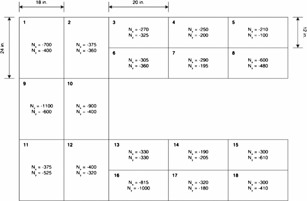
To demonstrate the feasibility of the optimisation method proposed, the example presented by Soremekun et al(Reference Soremekun, Gürdal, Kassapoglou and Toni30) consisting of 18 panels in a horseshoe configuration was used, as shown in Fig. 5. The local loads of each panel are assumed to be fixed and each panel is considered to have simply-supported boundary conditions. The objective is to find a fully blended design with all panels satisfying buckling constraints. Ply orientations are restricted to 0°, ±15°, ±30°, ±45°, ±60°, ±75° and 90°. The material used is a graphite-epoxy (IM7/8552) with E1 =141 GPa, E2 = 9.03 GPa, G12 = 4.27 GPa, μ12 = 0.32 and a ply thickness of 0.191 mm.
Eighteen-panel horseshoe configuration(Reference Soremekun, Gürdal, Kassapoglou and Toni30).

The value of λ corresponding to a buckling mode with m half-waves in the x direction and n half-waves in the y direction is
 $$\begin{equation}
\begin{array}{l} \lambda (m,n) = \{ {\pi ^2}[{D_{11}}{(m/a)^4} + 2({D_{12}} + 2{D_{66}}){(m/a)^2}{(n/b)^2}\\ {\rm{ }}\quad\quad\quad\quad\quad + {D_{22}}{(n/b)^4}]\} /\{ {(m/a)^2}{N_x} + {(n/b)^2}{N_y}\} \end{array},
\end{equation}$$
where a and b are the panel length and width, and D ij are the elements of the bending stiffness matrix for the plate obtained using classical lamination theory(Reference Soremekun, Gürdal, Kassapoglou and Toni30).
Two types of genetic algorithm are used, one for the optimisation process and the other for solving the stacking sequence of the guide laminate. For simplicity, the GA used for optimisation is marked as GA1 and the one used to solve the stacking sequence from lamination parameters as GA2. For both GA1 and GA2, a real-coded genetic algorithm is used.
4.1 Parameter set of GA1
For GA1, lamination parameters of the guide laminate and number of plies for each panel are design variables. For simplicity, only the bending lamination parameters of the guide laminate are used as design variables. To insure that the guide laminate are symmetric and balanced, VD 3 and VD 4 are set as 0. The bounds of the lamination parameters are (–1, 1), and (1, 24) for number of plies for each panel. The integer part of the real value is adopted to represent the number of plies; for example, if the real value of number of plies during real-coded genetic algorithm is 20.12, the number of plies used for calculating the lamination configuration is 20.
The GA1 code was processed with a population of 200, a 0.9 probability of crossover and a 0.05 probability of mutation. The master-slave parallel GA is adopted in this optimisation problem. The GA is performed on the high-performance IBM blade computer. There are 24 blades, and four processes of each blade are used.
4.2 Parameter set of GA2
For GA2, the number of plies is 48 as given by Adams et al( Reference Adams, Watson, Gürdal and Anderson-Cook 31 ), the stacking sequence of the guide laminate is optimised to target the lamination parameters of the guide. The total number of design variables is 24 (symmetric laminate). The laminate encoding method of Adams et al(Reference Adams, Watson, Gürdal and Anderson-Cook31) is used to force the laminate to be as close to balanced as possible (within one ply of each orientation). Real values from –7.5 to 97.5 represent the range of ply orientation. The range of (–7.5, 7.5) represents an orientation angle of 0°, (7.5, 22.5) for 15°, (22.5, 37.5) for 30°, (37.5, 52.5) for 45°, (52.5, 67.5) for 60°, (67.5, 82.5) for 75° and (82.5, 97.5) for 90°. Successive occurrences of a gene are mapped to the actual orientation angles with alternating plus and minus signs, starting from the centre of the (symmetric) laminate. For example, the first occurrence of a (7.5, 22.5) encoding maps to 15°, the second (7.5, 22.5) maps to –15°, and so on.
The GA2 code was also used with a population of 200, a 0.9 probability of crossover, a 0.05 probability of mutation and with 100 generations.
During the optimisation process, the buckling loads are calculated using an analytical formula. The buckling load multipliers λ cr are obtained by finding the lowest value of λ for all combinations of m and n. After Steps 1 and 2 of the optimisation process flowchart, the laminate configurations of each panel are calculated for buckling analysis. The effects of D ij are evaluated based on the stacking sequence and fibre angles of each panel.
For the balanced and symmetrical designs case, the best known feasible design with a weight of 28.91 kg is discovered by Yang(Reference Yang, Song, Zhong and Jin39). For the balanced and symmetrical designs design with outer blending, the best known design with a weight of 29.08 kg is obtained by Seresta(Reference Seresta, Abdalla and Gürdal32). Yang didn't use the conventional blending rule (a contiguous innermost (outermost) plies are deleted from the guide design). And the balanced condition is enforced by using stack variables, which means a 45° stack decodes to a ±45° ply as seen by Orest et al(Reference Seresta, Abdalla and Gürdal32). The decoding method of this paper is the same with Adams(Reference Adams, Watson, Gürdal and Anderson-Cook31) – that is, the successive occurrences of a gene are mapped to the actual orientation angles with alternating plus and minus signs, starting from the centre of the (symmetric) laminate. So the design discovered by Adams serves as a reference solution in this paper.
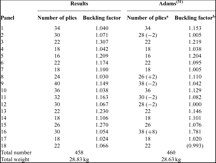
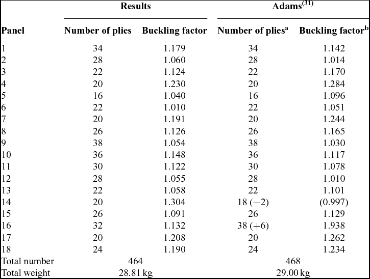
Tables 1 and 2 detail the optimum lamination parameters and real laminate configurations of each panel with inner blending. The resulting design contains two fewer plies (from 460 to 458) and weighs 28.83 kg compared to the 28.63 kg found by Adams(Reference Adams, Watson, Gürdal and Anderson-Cook31). But there is a failed panel from the results of Adams. Tables 3 and 4 detail the optimum lamination parameters and real laminate configurations of each panel with outer blending. Compared to the 29.00 kg found by Adams, a total weight of 28.81 kg is obtained while satisfying all the buckling constraints.
Lamination parameters and laminate configuration of optimum guide laminate with inner blending

Result comparison for laminates with inner blending

a Differences of ply numbers are marked between brackets.
b Failed panels are marked between square brackets. (The buckling factors of Adams were also evaluated by IJsselmuiden(Reference IJsselmuiden, Abdalla, Seresta and Gürdal40)).
Lamination parameters and laminate configuration of optimum guide laminate with outer blending

Result comparison for laminates with outer blending

a Differences of ply numbers are marked between brackets.
b Failed panels are marked between square brackets.
The optimum continuous guide lamination parameters are obtained with only bound constraints and no coupling relationship constraints of lamination parameters. The real lamination parameters of guide laminate are obtained using the least squares fitting method.
With parallel GA, the optimisation time has been reduced from 132 hours to about 90 minutes. Because the amount of information passed between processes is small and the calculation of an individual fitness needs a relatively large amount of time (about 24 seconds), the parallel GA obtains a nearly linear acceleration ratio.
The buckling optimisation panel problem only demonstrates that the method proposed works well for obtaining the blending laminate configurations but still needs many iterations using GA as an optimisation algorithm. However, the number of design variables of the method proposed is less than for the guide-based genetic algorithm method proposed by Adams. For this 18-panel test problem, the number of design variables of Adams(Reference Adams, Watson, Gürdal and Anderson-Cook31) is 40 (24 for guide laminate ply genes, 18 for ply counts of 18 panels). In the method proposed, the number of design variables decreased to 20 (two for lamination parameters of guide laminate, 18 for ply counts of 18 panels). For complicated engineering problems with many constraints (strength constraints, stiffness constraints, buckling constraints, etc.), compared with the two-level method proposed by IJsselmuiden, it maybe a little more time-consuming, but with a slightly better ability to obtain the global optimum and the convenience of including strength constraints. Compared with the conservative failure envelope for strength optimisation using lamination parameters(Reference IJsselmuiden, Abdalla and Gürdal44), the method of using real lamination parameters for strength analysis has a wider application scope.
5.0 CONCLUSIONS
Compared with the conventional guide-based blending genetic algorithm, using the lamination parameters of a guide laminate and number of plies of each panel as design variables in this paper can reduce the number of design variables, which is efficient for composite design engineering problems. Moreover, real laminate configurations (the laminate properties are defined by PCOMP cards instead of PSHELL and MAT2 cards in Nastran) of the panels are used for structure analysis instead of lamination parameters. The stress and strain information of each ply can be obtained, so the strength constraints (Tsai-Wu strength criteria, etc.) can easily be incorporated into the optimisation process compared with the conventional lamination parameter-based optimisation method. From the numerical example, the optimisation method presented in this paper has shown to be exceptionally effective for producing a blended design of composite panels with buckling constraints. And a parallel genetic algorithm shows a nearly linear acceleration ratio both in Jin et al(Reference Jin, Song and Zhong41) and in this paper.
One topic remains to be investigated in future work. Due to the excessive computational costs of the genetic algorithm, it is necessary to explore the proper mathematical programming algorithm used for optimisation.
ACKNOWLEDGEMENTS
The support for this work by the National Natural Science Foundation of China (11402204) and Fundamental Research Funds for the Central Universities of China (3102015BJ(II)ZS00) is gratefully acknowledged.