2. Equatorial coordinates of the sun

In this section, we will present all the formulae that are needed to determine the equatorial coordinates of the Sun, that is, the right ascension and the declination. The first thing that we need to calculate is the Julian date for the time of the observations.

The calendar that we use to count the time is cyclic repeating every 12 months. For some astronomical calculations, it is useful to have a linear count of the time. For that purpose, the Julian day number was created. The Julian day number is a continuous count of days from the beginning of the Julian period. The Julian day number 0 is assigned to the day starting at noon, Greenwich Mean Time, on the ${1}^{\rm{s}\rm{t}}$ of January of the year 4713 B.C. For example, the Julian day number for the day starting at 12h, Greenwich Mean Time, on the ${1}^{\rm{s}\rm{t}}$ of January of the year 2000, is 2451545. We will now explain how to determine the Julian date for a given day and time.

To calculate the Julian date (JD) of any given date and time, we first need to calculate the Julian day number (JDN). To obtain the Julian day number we proceed as followsFootnote ⁴ :

1. (i) express the date as YMD where Y is the year, M is the month number and D is the day in the month;

2. (ii) if the month is January or February subtract 1 from the year to get a new Y, and add 12 to the month to get a new M (we are thinking of January and February as being the last two months of the previous year).

Now, let

$$\eqalign{ {A } & = {\left\lfloor {{Y \over {100}}} \right\rfloor } \hfill & {} \hfill \cr {B} & = {\left\lfloor {{A \over 4}} \right\rfloor } \hfill & {} \hfill \cr {C} & = {\left\lfloor {2 - A + B} \right\rfloor } \hfill & {} \hfill \cr {E} & = {\left\lfloor {365.25(Y + 4716)} \right\rfloor } \hfill & {} \hfill \cr {F} & = {30.6001(M + 1)} \hfill & {} \hfill \cr {JDN} & = {C + D + E + F - 1524.5} \hfill & {} \hfill \cr } $$

The value obtained is the Julian day number of the given day at 0h Greenwich Mean Time. Finally, to determine the JD for a given day and time, let the time be given in hours (h), minutes (m) and seconds (s). The JD that we seek is given by the formula

$JD = JDN + {h \over {24}} + {m \over {1440}} + {s \over {86400}}$

Since the Julian date starts on January ${1}^{\rm{s}\rm{t}}$ of the year 4713 B.C., the number that we obtain for JD is quite large. Therefore, in astronomical calculations, it is common to use the Julian date for the ${1}^{\rm{s}\rm{t}}$ of January of 2000, and this value is obtained by subtracting the JD of the year 2000 that is equal to 2451545. Therefore,

$J{D}_{2000}=JD-2451545$

The next step is to compute the Sun’s coordinates, that is, the right ascension (RA) and declination ( $\delta $ ). For that, we do the following computations:Footnote ⁵

$\eqalign{ & {\rm{Mean\;anomaly\;of\;the\;Sun}}\!:\,\,\,\,\,\,\,\,\,\,\,\,\,\,\,\,\,\,\,\,\,\,\,\,\,\,\,\,\,\,\,\,\,\,\,\,\,\,\,\,\,\,\,\,\,\,\,\,\,\,\,\,\,\,\,\,\,\,\,\,g = 357.529 + 0.98560028J{D_{2000}} \cr & {\rm{Mean\;longitude\;of\;the\;Sun}}\!:\,\,\,\,\,\,\,\,\,\,\,\,\,\,\,\,\,\,\,\,\,\,\,\,\,\,\,\,\,\,\,\,\,\,\,\,\,\,\,\,\,\,\,\,\,\,\,\,\,\,\,\,\,\,\,\,\,q = 280.459 + 0.98564736J{D_{2000}} \cr & {\rm{Mean\;obliquity\;of\;the\;ecliptic}}\!:\,\,\,\,\,\,\,\,\,\,\,\,\,\,\,\,\,\,\,\,\,\,\,\,\,\,\,\,\,\,\,\,\,\,\,\,\,\,\,\,\,\,\,\,\,\,\,\,\,\,\,e = 23.439. - 0.00000036J{D_{2000}} \cr & {\rm{Geoccentric\;apparent\;ecliptic\;longitude\;of\;the\;Sun}}\!:\,\,L = q + 1.915\,{\rm{sin}}\,g + 0.020\,{\rm{sin}}\left( {2g} \right) \cr} $

All the constants are in degrees and the value of $L$ has to be reduced to the range ${0}^{\circ }$ to $36{0}^{\circ }$ . Finally, the Sun’s right ascension (RA) and declination ( $\delta $ ) can be obtained from the formulae

$$RA = {\rm{arctan}}\left( {\frac{{{\rm{cos}}\;e\;{\rm{sin}}\;L}}{{{\rm{cos}}\;L}}} \right)$$

$\!\!{\delta = {\rm{arcsin}}\left( {{\rm{sin}}\ e\ {\rm{sin}}\ L} \right)}$

3. Gauss’ method

One of the most important problems in celestial navigation is the one of determining the ship’s position at sea. By the end of the 18th century, it was possible to determine the latitude and longitude at sea with good accuracy. However, the coordinates were determined at different times, the latitude was calculated at the exact moment of the Sun’s meridian passage and the longitude was calculated at a time close to the Sun’s rising or setting using the time-sight method. The fact that the coordinates were determined at different times of the day was clearly a disadvantage.

In 1809, Gauss proposed a method to determine the ship’s position based on the observation of two stars. The method is described in the book 100 Great Problems in Elementary Mathematics written by Heinrich Dorrie (Dorrie, Reference Dorrie1965). The original text was written in Latin and a translation to German can be found in Astronomisches Jahrbuch published by J. E. Bode in 1809 (Bode, Reference Bode1809).

Gauss’ proposal is based on the altitudes of two stars observed simultaneously. The positions of these stars would be marked on the celestial sphere using the right ascension and declination of both of them. The difference between the right ascensions defines one of the angles of the spherical triangle whose vertices are the celestial pole and the positions of the stars. However, this process can also be used with two altitudes of the Sun at two different instants. In this section, we will present Gauss’ method in the case when we use two altitudes of the Sun.

Let $h$ and $h\rm{\text{'}}$ denote the two altitudes of the Sun taken at two different instants. In this method, it is assumed that both altitudes are observed in the same place, but since this is not the case if the ship is navigating, then the altitude taken at the first observation has to be reduced to the place where the second altitude was observed. We will describe this process by following the explanation presented by Dorrie (Reference Dorrie1965, pp. 326–327).

Suppose the first altitude was taken at place $A$ at a given time and the second altitude was taken at place $B$ at another time. We need to determine the altitude of the Sun at place $B$ at the time of the first observation.

First, recall that all places on the earth’s surface which have an equal altitude of the Sun at the same instant of time lie on a circle called the equal altitude circle of the Sun.

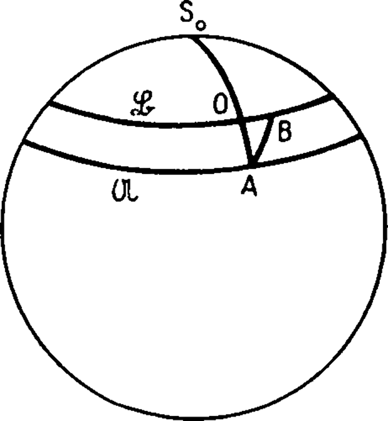
In Figure 1, let $\mathcal{U}$ and $\mathcal{L}$ be the two equal altitude circles of the star at time $t$ on which the observation points $A$ and $B$ lie; let ${S}_{0}$ be the Sun image and $O$ the point of intersection of the great arc ${S}_{0}A$ with $\mathcal{L}$ . Since the distance $AB$ is relatively small, we can assume that the triangle $AOB$ is plane. We obtain the difference between the zenith distances and, consequently, also for the difference in the altitudes of the Sun at $A$ and $B$ :

$AO=AB\ \rm{c}\rm{o}\rm{s} \; \omega$

where $\omega $ is the angle between the ship’s course $AB$ and the bearing $AO$ of the Sun at $A$ .

Figure 1.

A diagram showing how to reduce the altitude of the star observed at time A to time B.

Source: Dorrie (Reference Dorrie1965), p. 326.

Thus, the Sun’s altitude at $B$ at the time of the first observation can be obtained as follows.

If the ship draws near the Sun, then increase the value of the Sun’s altitude at place $A$ by the quantity $AB\ \rm{c}\rm{o}\rm{s}\ \omega $ , else decrease it by $AB\ \rm{c}\rm{o}\rm{s} \; \omega $ . After calculating the reduced altitude for the first observation, replace the value of $h$ by the value obtained.

After correcting the first observed altitude to the place of the second observation, we will now describe Gauss’ method to determine the latitude. Recall that $h$ denotes the value of the Sun altitude for the first observation after the correction described in the previous paragraph, $h\rm{\text{'}}$ denotes the Sun altitude at the time of the second observation and $\varphi$ denotes the latitude at the time of the second observation.

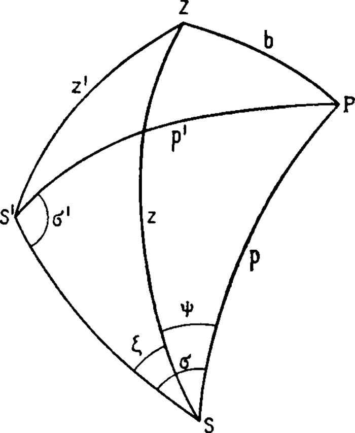
In Figure 2, let $S$ and $S\rm{\text{'}}$ be the places of the Sun at the times of the observations, with $S$ being the place for the second observation and $S\rm{\text{'}}$ for the first. Their equatorial coordinates are the right ascension, denoted by $RA$ and $R{A}{\rm{\text{'}}},$ and the declination denoted by $\delta $ and $\delta \rm{\text{'}}$ , respectively. Let $P$ be the North pole; thus $PS=p=9{0}^{\circ }-\delta $ is the polar distance from $S$ ; similarly $PS\rm{\text{'}}=p\rm{\text{'}}=9{0}^{\circ }-\delta \rm{\text{'}}$ .

Figure 2.

Spherical triangles containing the pole, the observer’s zenith and the positions of the two stars.

Source: Dorrie (Reference Dorrie1965), p. 324.

Let $\tau $ be the angle between the hour circles of the two places of the Sun, as well as the magnitude of the right ascension difference. Let $Z$ be the zenith of the observation point, so that $PZ=b=9{0}^{\circ }-\varphi$ is the complement of the latitude, $ZS=z=9{0}^{\circ }-h$ is the zenith distance from $S$ and $ZS {\text{'}}=z{\text{'}}=9{0}^{\circ }-h{\text{'}}$ is the zenith distance from $S{\text{'}}$ .

It is still necessary to determine the following quantities: ${\measuredangle }{\rm PSS}{\text{'}}=\sigma $ , ${\measuredangle }{\rm PS}{\text{'}}{\rm S}=\sigma {\text{'}}$ , ${\measuredangle} {\rm PSZ}=\psi $ , ${\measuredangle} {\rm ZSS}{\text{'}}=\zeta $ and the side $SS{\text{'}}={s}$ .

Using the triangle $PS{S}{{\text{'}}},$ we can determine the angles $\sigma $ and $\sigma {\text{'}}$ . By Napier’s formulaeFootnote ⁶ , we have

${{\rm{tan}}{{\sigma + \sigma {\rm{'}}} \over 2} = {{{\rm{cos}}{{p{\rm{'}} - p} \over 2}} \over {{\rm{cos}}{{p{\rm{'}} + p} \over 2}}}{\rm{cot}}\left( {{\tau \over 2}} \right){\rm{\,\,\,\,and\,\,\,\,tan}}{{\sigma - \sigma {\rm{'}}} \over 2} = {{{\rm{sin}}{{p{\rm{'}} - p} \over 2}} \over {{\rm{sin}}{{p{\rm{'}} + p} \over 2}}}{\rm{cot}}\left( {{\tau \over 2}} \right)}$

By solving the above system of equations, we conclude that

(1) $\eqalign{ {\sigma = {\rm{arctan}}\ \left[ {{{{\rm{cos}}{{p{\rm{'}} - p} \over 2}} \over {{\rm{cos}}{{p{\rm{'}} + p} \over 2}}}{\rm{cot}}\left( {{\tau \over 2}} \right)} \right] + {\rm{arctan}}\ \left[ {{{{\rm{sin}}{{p{\rm{'}} - p} \over 2}} \over {{\rm{sin}}{{p{\rm{'}} + p} \over 2}}}{\rm{cot}}\left( {{\tau \over 2}} \right)} \right]} \hfill \cr {\sigma {\rm{'}} = {\rm{arctan}}\ \left[ {{{{\rm{cos}}{{p{\rm{'}} - p} \over 2}} \over {{\rm{cos}}{{p{\rm{'}} + p} \over 2}}}{\rm{cot}}\left( {{\tau \over 2}} \right)} \right] - {\rm{arctan}}\ \left[ {{{{\rm{sin}}{{p{\rm{'}} - p} \over 2}} \over {{\rm{sin}}{{p{\rm{'}} + p} \over 2}}}{\rm{cot}}\left( {{\tau \over 2}} \right)} \right]} \hfill \cr {} \hfill \cr } $

The side $s$ can be determined by the formula

${{{\rm{sin}}\ s} \over {{\rm{sin}}\ p}} = {{{\rm{sin}}\ \tau } \over {{\rm{sin}}\ \sigma '}}$

that is,

(2) $s = {\rm{arcsin}}\ \left( {{{{\rm{sin}}\ \tau } \over {{\rm{sin}}\ \sigma {\rm{'}}}}{\rm{sin}}\ p} \right)$

Using the triangle $ZS{S}^{\rm{\text{'}}},$ we can determine the angle $\zeta $ according to the tangent theorem for the half angle:

${\rm{tan}}{\zeta \over 2} = \sqrt {{{{\rm{sin}}\left( {{\rm{\Sigma }} - z} \right){\rm{sin}}\left( {{\rm{\Sigma }} - s} \right)} \over {{\rm{sin\ \Sigma \;sin}}\left( {{\rm{\Sigma }} - z{\rm{'}}} \right)}}} $

where ${\rm{\Sigma }} = {{z + z{\rm{'}} + s} \over 2}$ , that is,

(3) $\zeta = 2\,{\rm{arctan}}\ \left[ {\sqrt {{{{\rm{sin}}\left( {{\rm{\Sigma }} - z} \right)\ {\rm{sin}}\ \left( {{\rm{\Sigma }} - s} \right)} \over {{\rm{sin\,\Sigma \,sin}}\left( {{\rm{\Sigma }} - z{\rm{'}}} \right)}}} } \right]$

Now, we can determine

(4) $\psi =\sigma -\zeta .$

The latitude can be obtained from

${\rm{c}}{\rm{o}}{\rm{s}}\ b={\rm{c}}{\rm{o}}{\rm{s}}\ p\ {\rm{c}}{\rm{o}}{\rm{s}}\ z+{\rm{s}}{\rm{i}}{\rm{n}}\ p\ {\rm{s}}{\rm{i}}{\rm{n}}\ z\ {\rm{c}}{\rm{o}}{\rm{s}}\ \psi .$

and since $b=9{0}^{\circ }-\varphi, $ we have

${\rm{s}}{\rm{i}}{\rm{n}}\ \varphi ={\rm{c}}{\rm{o}}{\rm{s}}\ p\ {\rm{c}}{\rm{o}}{\rm{s}}\ z+{\rm{s}}{\rm{i}}{\rm{n}}\ p\ {\rm{s}}{\rm{i}}{\rm{n}}\ z\ {\rm{c}}{\rm{o}}{\rm{s}}\ \psi .$

that is,

(5) $\varphi ={\rm{arcsin}}\ \left({\rm{cos}}\ p\ {\rm{cos}}\ z+{\rm{sin}}\ p\ {\rm{sin}}\ z\ {\rm{cos}}\ \psi \right)$

The latitude obtained is the latitude at the time and place of the second observation. Furthermore, if the value is positive, then the latitude is North, otherwise is South.

We now need to determine the longitude. The longitude can be determined by calculating the time difference between the local apparent time (LAT)Footnote ⁷ and the Greenwich apparent time (GAT). The time difference between these two, when converted to degrees, is the value of the longitude at the ship’s location.

In Figure 2, let $t={\measuredangle }\,{{ZPS}}$ , then

${\rm{cos}}\ t = {{{\rm{sin}}\ h - {\rm{sin}}\ \delta\ {\rm{sin}}\ \varphi } \over {{\rm{cos}}\ \delta\ {\rm{cos}}\ \varphi }}$

thus,

(6) $t = {\rm{arccos}}\ \left( {{{{\rm{sin}}\ h - {\rm{sin}}\ \delta\ {\rm{sin}}\ \varphi } \over {{\rm{cos}}\ \delta\ {\rm{cos}}\ \varphi }}} \right).$

Next, we convert the value of $t$ to time and denote it by ${t}^{\rm{*}}$ . We have ${t}^{\rm{*}}=t/15$ , since 1 hour corresponds to 15°.

We now need to determine the local apparent time (LAT). If the Sun observation was made in the morning, subtract ${t}^{\rm{*}}$ from 12h, otherwise add the obtained time to 12h. That is,

(7) $\matrix{ {LAT = 12 - {t^{\rm{*}}}{\rm{\,if\,AM\;observation}}} \hfill \cr {LAT = 12 + {t^{\rm{*}}}{\rm{\,\,if\;PM\,observation}}} \hfill \cr } $

The next step will be to determine the corresponding Greenwich hour angle, denoted by GHA, of a given time observation of the Sun. To determine the value of the GHA, we need to know the Julian Date for the year 2000 for that time, denoted by $J{D}_{2000}$ , and the Sun’s right ascension at that time, denoted by $RA$ . Recall that an explanation on how to determine $J{D}_{2000}$ and $RA$ can be found in Section 2. Therefore, to obtain the value of $GHA$ of a given observation time, do the following calculations:

1. (a) $T = {{J{D_{2000}}} \over {36525}}$

2. (b) \begin{array}{*{20}{c}}{GH{A_{Aries}} = 280.46061837{\rm{ + }}360.98564736629J{D_{2000}}{\rm{ + }}\frac{{0.000387933{T^3}}}{{38710000}}} \hfill\\\end{array}

3. (c) $GHA=GH{A}_{Aries}+360-RA$

Let GHA* be the Greenwich hour angle converted to the interval from 0° to 360°. Then, GHA ${\rm{}}^{\rm{*}}$ can be obtained by the formula

${\rm{If\;}}GHA \lt 360,\;{\rm{\;then\;}}GH{A^{\rm{*}}} = GHA,\;\;{\rm{else\;}}GH{A^{\rm{*}}} = GHA - 360.$

Now, we need to determine the Greenwich apparent time (GAT).

(8) $${\rm{If}}\,GH{A^{\rm{*}}}{\rm{ > }}180, \, {\rm{then}}\,GAT = 12 - \frac{{360 - GH{A^{\rm{*}}}}}{{15}},\,\,{\rm{else}}\,GAT = 12{\rm{ + }}\frac{{GH{A^{\rm{*}}}}}{{15}}.$$

Finally, the value of the longitude in degrees is given by

(9)

4. Gauss’ method practical application

In this section, our aim is to see how the method proposed by Gauss behaves in practise. For that purpose, the method was implemented in an Excel spreadsheet. Before we explain each step, we need to define the initial variables and make some comments. Let ${h}_{1}$ and ${h}_{2}$ denote the two altitudes of the Sun, and let ${t}_{1}$ and ${t}_{2}$ denote the time of the observations, respectively. As observed before, the method assumes that both altitudes were taken at the same place. Therefore, the altitude taken at the first observation has to be reduced to the place where the second altitude was observed. The procedure to correct the altitude was explained in Section 3. Thus, from now on, and for the sake of simplicity, we assume that ${h}_{1}$ denotes the value of the first altitude corrected to the place of the second altitude. At the time of the observations, let the Sun’s declination be denoted by ${\delta }_{1}$ and ${\delta }_{2},$ and let the right ascension be denoted by $R{A}_{1}$ and $R{A}_{2}$ . Let $\varphi $ and $L$ denote the latitude and longitude determined by the algorithm, and let ${\varphi }_{GPS}$ and ${L}_{GPS}$ denote the GPS latitude and longitude for the time of the second observation. Observe that the arguments of all trigonometric functions in Excel are in radians; therefore, all decimal angles have to be converted to radians.

The first thing that we need to do is to determine the Greenwich hour angle of the observation times of ${h}_{1}$ and ${h}_{2}$ , which we will denote by ${\tau }_{1}$ and ${\tau }_{2}$ respectively. To determine the value of the Greenwich hour angle, we need to know the Julian Date for the year 2000, denoted by $J{D}_{2000}$ of the time and the Sun’s right ascension at that time, denoted by $RA$ . Recall that an explanation on how to determine $J{D}_{2000}$ and $RA$ can be found in Section 2. Therefore, to obtain the value of ${\tau }_{1}$ that corresponds to the Greenwich hour angle of ${t}_{1},$ do the following calculations and then repeat to obtain the value of ${\tau }_{2}$ :

1. (a) ${T_1} = {{J{D_{2000}}\left( {{t_1}} \right)} \over {36525}}$

2. (b) $GH{A_{Are{s_1}}} = 280.46061837 + 360.98564736629J{D_{2000}}\left( {{t_1}} \right) + {{0.000387933T_1^3} \over {38710000}}$

3. (c) ${\tau }_{1}=GH{A}_{Arie{s}_{1}}+360-R{A}_{1}$

We will now list all the steps that we have implemented in the Excel spreadsheet to determine the latitude at the time of the second observation:

$\eqalign{ & z = Radians\left( {90 - {h_1}} \right) \cr & z{\rm{'}} = Radians\left( {90 - {h_2}} \right) \cr & p = Radians\left( {90 - {\delta _1}} \right) \cr & p{\rm{'}} = Radians\left( {90 - {\delta _2}} \right) \cr & \tau = Radians\ \left( {{{{\tau _2} - {\tau _1}} \over 2}} \right) \cr & \sigma = {\rm{arctan}}\ \left[ {{{{\rm{cos}}{{p{\rm{'}} - p} \over 2}} \over {{\rm{cos}}{{p{\rm{'}} + p} \over 2}}}{\rm{cot}}\left( {{\tau \over 2}} \right)} \right] + {\rm{arctan}}\ \left[ {{{{\rm{sin}}{{p{\rm{'}} - p} \over 2}} \over {{\rm{sin}}{{p{\rm{'}} + p} \over 2}}}{\rm{cot}}\left( {{\tau \over 2}} \right)} \right] \cr & \sigma {\rm{'}} = {\rm{arctan}}\ \left[ {{{{\rm{cos}}{{p{\rm{'}} - p} \over 2}} \over {{\rm{cos}}{{p{\rm{'}} + p} \over 2}}}{\rm{cot}}\left( {{\tau \over 2}} \right)} \right] - {\rm{arctan}}\ \left[ {{{{\rm{sin}}{{p{\rm{'}} - p} \over 2}} \over {{\rm{sin}}{{p{\rm{'}} + p} \over 2}}}{\rm{cot}}\left( {{\tau \over 2}} \right)} \right] \cr & s = {\rm{arcsin}}\ \left[ {{{{\rm{sin}}\ \tau\ {\rm{sin}}\ p} \over {{\rm{sin}}\ \sigma {\rm{'}}}}} \right] \cr & {\rm{\Sigma }} = {{z + z{\rm{'}} + s} \over 2} \cr & \zeta = 2\ {\rm{arctan}}\ \left[ {\sqrt {{{{\rm{sin}}\left( {{\rm{\Sigma }} - z} \right)\ {\rm{sin}}\ \left( {{\rm{\Sigma }} - s} \right)} \over {{\rm{sin}}\left( {\rm{\Sigma }} \right)\ {\rm{sin}}\ \left( {{\rm{\Sigma }} - z{\rm{'}}} \right)}}} } \right] \cr & \psi = \sigma - \zeta \cr & \varphi = {\rm{arcsin}}\ \left( {{\rm{cos}}\ p\ {\rm{cos}}\ z + {\rm{sin}}\ p\ {\rm{sin}}\ z\ {\rm{cos}}\ \psi } \right) \cr} $

If the value of $\varphi $ obtained is positive, then the latitude is North, otherwise it is South.

Having determined the latitude, we need to calculate the longitude for the time of the second observation. We will now list the steps that we have done in our Excel spreadsheet:

The aim of this section is to analyse the reliability of this method. For that purpose, we have applied the algorithm described above to determine the latitude and longitude using real observations of the Sun at sea, and the results obtained were compared with the GPS values.

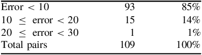
In 2021 and 2022, we travelled on board the Portuguese Navy’s tall ship Sagres and collected 109 pairs of Sun’s altitudes. The altitudes were taken using a sextant and were corrected for index error, dip, refraction and parallax. The times of the observations were also registered as well as the GPS position. For each pair, the first altitude was corrected to the place of the second altitude, as described in Section 3. The algorithm was performed on an Excel spreadsheet and the values of the latitude and longitude obtained were compared with the GPS values. The values of the longitude obtained all had an error less than 1 minute when compared with the GPS longitude. As for the latitude, we obtained 93 pairs with an error less than 10 miles which correspond to 85% of the total pairs. The largest error was 22.7 miles and the smallest was 0.02 miles. A more detailed summary of the results obtained can be found in Table 1.

Table 1.

Results obtained by Gauss’ method.

From the results obtained, we conclude that the method proposed produces good results and can be seen as an alternative method for emergency navigation when GNSS fails and other navigation methods need to be used.

Another aim of the paper is to see how the algorithm behaves when there is no influence of observation errors. For that purpose, for each pair, we have determined the Sun’s true altitude for the time of the observation and the GPS position. Knowing the GPS latitude, the Sun’s declination and the local hour angle (LHA), the true altitude of the Sun at that time and place, denoted by $a$ , can be determined by the following formula:

(10) $$a = {\rm{arcsin}}\;\left( {{\rm{sin}}\;{\varphi _{GPS}}\;{\rm{sin}}\;\delta {\rm{ + cos}}\;{\varphi _{GPS}}\;{\rm{cos}}\;\delta \;{\rm{cos}}\left( {LHA} \right)} \right)$$

Thus, using Equation (10), we have determined the true altitudes of the Sun for the two observations times. Recall that the value of the Sun’s declination was determined using the procedure described in Section 2 and the value of LHA was already determined before since this value is needed in the algorithm to determine the longitude.

We have run the algorithm again using the Sun’s true altitudes instead of the altitudes observed. For the 109 pairs considered, the values obtained for the latitude and longitude were exactly the same as the registered GPS values, that is, the error was equal to zero. This proves that the algorithm calculates the exact latitude and longitude if the input values are free from the influence of observational errors. Therefore, the algorithm presented is a good alternative to determine the ship’s position whenever the GNSSs fail and one needs alternative navigation methods.