

Introduction
Knowledge and monitoring of the grapevine phenology during the season are important requirements for planning various production activities at the vine field scale (Mullins et al., Reference Mullins, Bouquet and Williams1992). For example, practices such as fertilization, irrigation, application of phytosanitary products and harvest are programmed based on the evolution of the grapevine phenology. For a correct planning of the practices mentioned above, the wine growers need to know in advance the date of occurrence of the key phenological stages such as budburst, flowering and veraison. Traditionally, the evolution of the grapevine phenology is related to climatic variables, specifically with air temperature (Chuine et al., Reference Chuine, García de Cortazar-Atauri, Kramer and Hänninen2013). Through this relation, classical climatic models of phenology have been proposed in the literature (Chuine et al., Reference Chuine, García de Cortazar-Atauri, Kramer and Hänninen2013). These climatic models predict the date of occurrence of the key phenological stages using air temperature as the only variable. Temperature data used for these models come from meteorological stations or service providers. Whatever their origin, meteorological data are usually available at a medium to low spatial resolution, therefore depending on the location of a field (and environmental attributes), air temperature used to run the models may differ from air temperature really experienced by the field. In addition, data resolution is too low to work at the within field scale, as a result, meteorological data are generally applied at the vineyard or field scale. Therefore, climatic models provide generally an average value of the date of occurrence of the phenological stage which is extrapolated to the whole vineyard without considering the spatial variability.
Previous studies have shown that within-field variability of grapevine phenology may be significant and may justify site-specific management practices (Verdugo-Vásquez et al., Reference Verdugo-Vásquez, Acevedo-Opazo, Valdés-Gómez, Araya-Alman, Ingram, García de Cortázar-Atauri and Tisseyre2015a). Therefore, under conditions of high spatial variability, the extrapolation of the average value obtained through the climatic models may not be representative of the whole fields.
An alternative approach to solve the above problem is to use a spatial model. The spatial model allows the estimation of a variable over the whole field taking into account the spatial variability. Spatial models have been used successfully to estimate vine water status under non-irrigated (Acevedo-Opazo et al., Reference Acevedo-Opazo, Tisseyre, Ojeda and Guillaume2010) and irrigated conditions (Acevedo-Opazo et al., Reference Acevedo-Opazo, Valdés-Gómez, Taylor, Avalo, Verdugo-Vásquez, Araya and Tisseyre2013). It has also been used more recently to estimate the precocity (delay or advance of the date of occurrence of phenological stages with respect to a reference site) of the grapevine phenology (Verdugo-Vásquez et al., Reference Verdugo-Vásquez, Acevedo-Opazo, Valdés-Gómez, Araya-Alman, Ingram, García de Cortázar-Atauri and Tisseyre2015b). Therefore, spatial models allow the characterization of the spatial variability of the fields through a single measurement on the field (reference site) and a combination of site-specific coefficients calculated through historical data.
The combination of the classical climate model of phenology and a spatial model would allow predicting the date of occurrence of the grapevine phenology taking into account the spatial variability of the field. For this, the climate model is used to predict the date of occurrence of the phenological stage (for example: budburst, flowering or veraison). This information is incorporated in the spatial model as the measurement of the reference site, allowing to extrapolate estimated date of occurrence to the whole field. This approach has not been tested for the grapevine phenology. In literature, information about spatio-temporal modeling of the grapevine phenology at the within-field scale is scarce. There is a spatio-temporal model of phenology, but developed to work at regional scale (Mariani et al., Reference Mariani, Alilla, Cola, Monte, Epifani, Puppi and Osvaldo2013). This model uses climatic data, specifics observations of phenology and geo-statistical analyzes to predict temporally and spatially the phenology at the regional scale.
The aim of this work is to calibrate and validate an empirical approach to predict the date of occurrence of the grapevine phenology temporally and spatially at the within-field scale. The goal is also to characterize the different sources of inaccuracy when mixing a spatial model with a temporal model and to test its relevancy on a real phenological data set.
Materials and methods
Fields charateristics and measurements
The experiment was performed on a field of cv Cabernet Sauvignon (1.56 ha) located in the Panguilemo Experimental Station of the University of Talca (Maule Valley), Chile, under irrigated conditions. The phenological observations were estimated using the Eichhorn and Lorenz phenological scale as modified by Coombe (Coombe Reference Coombe1995). Measurements of the date of occurrence of the grapevine phenology (budburst, flowering and veraison) were performed on each site of a regular sampling grid (18 sites) during 4 consecutive seasons (from 2009–10 to 2012–13 season). Climate data (air temperature) were collected using an automatic weather station (Adcon Telemetric, A730, Klosterneuburg, Austria) installed under reference conditions, at 300 m from the vineyards. Air temperature were measured at 15-min intervals.
Spatio-Temporal model of the grapevine phenology
a) The temporal model
In this study, the Growing Degree Day model (GDD model) was used to predict the date of occurrence of phenological stages (PS) of budburst, flowering and veraison. This model assumes that the date of occurrence t s (day of the year, DOY) of a phenological stage (Date PS ) occurs when a critical state of forcing S f , defined as a sum of growing degree days from a starting date t 0 , reached a particular value F* (Eq. 1) (García de Cortázar-Atauri et al., Reference García de Cortázar-Atauri, Brisson and Gaudillere2009; Parker et al., Reference Parker, García de Cortázar-Atauri, Chuine, Barbeau, Bois, Boursiquot and van Leeuwen2013).
 $$S_{f} \left( {t_{s} } \right)\,{\equals}\,\mathop{\sum}\nolimits_{t_{0} }^{t_{s} } {GDD(x_{t} )\,{\equals}\,F^{{\rm {\asterisk}}} } $$
The state of forcing is described as a daily sum of the rate of forcing, (Eq. 2) which starts at t 0 , x t is the daily mean temperature and Tb corresponds to a base temperature above which the thermal summation is calculated.
 $$GDD\left( {x_{t} } \right)\,{\equals}\,\left\{ {\matrix{ 0 & {if\quad {\rm }x_{t} \,\lt\,T_{b} } \cr {x_{t} {\minus}T_{b} } & {if\quad {\rm }x_{t} \geq T_{b} } \cr } } \right\}$$
This approach has three parameters: t 0 , F* and Tb. Parameters values used in this study are shown in Table 1.
Parameters values considered for the climatic model (GDD model, Eqs. 1 and 2)

For the computation of GDD (Eq. 2) information of air temperature collected by the automatic weather station were used. The date predicted by the climate model (Date PS ) corresponds to the days of the year t s when GDD reach the value F*. In order to take into account possible differences between field climatic conditions and weather station located more than 300 m away, a correction parameter C was introduced in the climatic model (Eq. 3). The correction coefficient C was expressed in days, it was determined by computing the difference between the average observed date of occurrence of the phenological stage (all sites) and the date predicted by the climatic model (mean of the first 3 seasons for each phenological stage).
 $$C\,{\equals}\,\bar{X}{\rm }\,\left[ {Date_{{\overline{{PS}} }} \left( {All\,sites} \right)\,{\minus}\,Date_{{PS}} } \right]$$
Once determined C, was incorporated (adding or subtracting) on the date estimated with the climatic model (GDD Model). The resulting corrected climatic model (Eq. 4) was called temporal model in the rest of the document.
 $$Date_{{PS}} \,Climatic\,{\equals}\,Date_{{PS}} \,\pm\,C$$
b) The spatial model
The approach used in this work was the one proposed by (Acevedo-Opazo et al., Reference Acevedo-Opazo, Tisseyre, Ojeda and Guillaume2010) successfully applied to model the spatial variability of vine water status at the within field scale. The aim of the spatial model is to produce an estimate of the date of occurrence of the phenological stage PS on site s
i
 $(Date_{{PS}} \hat{S}_{i} )$
, from a reference site
 $Date_{{PS}} s_{{ref}} $
. This estimation is performed using a simple linear function. (Eq. 5). The spatial model corresponded to a spatial extrapolation that allows modelling the relative differences of the date of occurrence of the phenological stage (PS) between each site s
i
and the reference site s
ref
. This model predicts the precocity of the phenological stage (PS) of the grapevine by considering the delay or the advance of the date of occurrence of the PS with respect to a reference site s
ref
. It was applied at the vine field scale. The spatial model is based on a collection of linear coefficients
 $a_{{S_{i} }} {\rm }$
( Eq. 5) called vector a.
 $$Date_{{PS}} \,\hat{S}_{i} \,{\equals}\,a_{{s_{i} }} \,{\rm x}\,Date_{{PS}} \,S_{{ref}} $$
Estimation of
 $a_{{S_{i} }} $
requires historical information of the date of occurrence of the phenological stage at the vine field scale. In this study, a value of
 $a_{{S_{i} }} $
for each phenological stage (budburst, flowering and veraison) was calculated.
In this approach, a virtual site was added to the database, corresponding to the average (all sites of the field) date of occurrence of each PS calculated for each date. This virtual site was then considered as the reference site (s
ref
) for the calculation of
 $a_{{S_{i} }} $
of the spatial model.
c) Spatio-Temporal model
Finally, assuming the date estimated by the temporal model (Date PS Climatic) component corresponded to the average phenological stage of the field, the Spatio-Temporal model was defined by considering Date PS Climatic value as the reference site (Eq. 6).
 $$Date_{{PS}} \,\hat{S}_{i} \,{\equals}\,a_{{s_{i} }} \,{\rm x}\,Date_{{PS}} \,Climatic$$
Calibration and validation of the different models
The different models (GDD Model, Temporal, Spatial and Spatio-Temporal) were calibrated using data collected during the first 3 seasons. A fourth season was used as a validation dataset to evaluate the ability of prediction with data not used to calibrate the model. For both processes (calibration and validation), the root mean square error (RMSE) was used to characterize the accuracy of each model for each phenological stage. Additionally, the observed standard deviation of the field was considered as a reference value for all the phenological stages. This standard deviation corresponds to the RMSE when the mean of all sites is used to estimate the phenological stage of the field. In this study, the standard deviation was considered to characterize the error when a very simple model of estimation corresponding to the mean is considered.
Differences (expressed in days) between observed date of occurrence of the phenological stage and estimated date for the temporal and spatial component were also calculated (validated process) for each site of the sampling grid. These differences were used to show potential spatial patterns in error either for the temporal model or the spatial model. Errors were mapped in 33% quantiles for each phenological stage, using the 3D-field software (version 2.9.0.0., Copyrigtht 1998-2007, Vladimir Galouchko, Russia).
Results and discussion
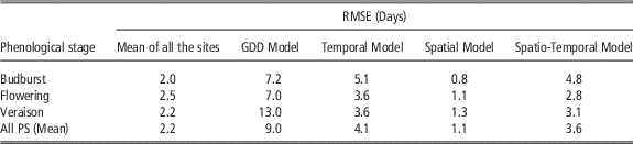
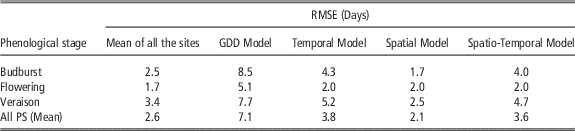
Table 2 and 3 shows the RMSE obtained by the different approaches for calibration and validation processes, respectively. For both processes, the GDD and temporal model shows the highest RMSE values, while the lowest RMSE value is obtained with the spatial model. For almost all cases, the RMSE values obtained by the GDD model were similar or lower than those obtained under the calibration conditions of these models (García de Cortázar-Atauri et al., Reference García de Cortázar-Atauri, Brisson and Gaudillere2009; Parker et al., Reference Parker, García de Cortázar-Atauri, Chuine, Barbeau, Bois, Boursiquot and van Leeuwen2013). Note that, the incorporation of the C in the Temporal model improved the result of the GDD model. Focusing on the average RMSE observed over all seasons (last row in Tables 2 and 3), note that the order of the models is always the same. The spatial model always has the lowest RMSE, followed by the mean model. Models integrating the temporal component (based on temperature) systematically present significantly higher errors. The integration of a spatial model makes it possible to slightly improve the error during the calibration. This improvement is perceptible during the prediction but it is much less marked. In general, the higher RMSE values observed for the GDD and temporal models may be explaind by the fact that these models predicts the date of occurrence of the phenological stage with indirect information (air temperature), while other models (Mean of all the sites and Spatial model) use measurements of phenology performed in the field to estimate the values of the other sites.
Errors (RMSE) of calibration obtained by the different model approaches

Errors (RMSE) of prediction obtained by the different model approaches

There is a very small increase in RMSE between calibration and prediction steps. This result was expected for the mean model since there is no strictly speaking a prediction for this model which takes into account the observations made over the field whatever the considered step. On the other hand, this result highlights the ability of all other models to predict the phenology of the field on data that are not used for model calibration.
The precision of the models is different according to the phenological stages considered. If the mean and spatial models show the best results for all the stages, the temporal models predict very well the flowering and worse the veraison. This aspect may be of interest from a practical point of view, since depending on the expected accuracy different approaches can be considered for each phenological stage.
This work will focus on the study of the models and will not take into account the operational aspects. Note however, that a 5-day error on phenology estimation may be sufficient for many applications and that the choice of a more precise estimation method should necessarily take into account the operational constraints. These constraints differ greatly from one method to another. For example, the average model requires observations to be made on all sites systematically, the spatial model and the spatio-temporal models require a single observation on a reference site (provided that a historical database is available for their calibration).
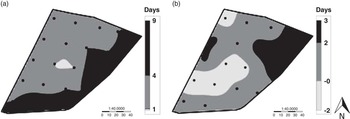
Regarding the spatial error, Figure 1 shows the maps of the spatial error (expressed in days) of the phenological stage of budburst (validation process) obtained for the temporal (a) and spatial (b) model. It is observed that the distribution of the errors for the temporal model has a high spatial structure, where the highest errors (>4 days) are distributed in the southern part of the field (Fig. 1 a). On the other hand, for the spatial model, errors are more randomly distributed (Fig. 1 b) and never exceed 3 days. For the temporal model, only positive values of error are observed, therefore, this model underestimates the date of occurrence of the phenological stage of budburst. This result shows that the correction coefficient (Eq. 4) may not be sufficient to model the eventual difference between field conditions and weather station conditions. For the spatial model, errors are centered on 0 showing that integration of observations performed on the field limit bias (over or under estimation). Very similar results were observed for flowering and veraison stages, (data not shown). In summary, for these phenological stage, the temporal model overestimates the date of occurrence.
Maps of the spatial error (expressed in days) of the phenological stage of budburst (validation process) obtained for the temporal (a) and spatial (b) model.

The incorporation of the spatial component in the spatio-temporal model (
 $a_{{S_{i} }} $
, Eq. 7) allows for the randomized distribution in the field of the date of occurrence estimated by the temporal model (Date
PS
Climatic, Eq. 7). This improves the results obtained when considering only the temporal model (Tables 2 and 3). However, to obtain better results with the spatio-temporal model it is necessary to improve the estimation of the value of the reference site, that is to say, of the temporal model. These results show that the main sources of imprecision come from the temporal model which must be “reset” in relation to the particular conditions of the field. Two ways of improvement can be envisaged. One is based on the use of weather stations (sensor networks) located within the field to benefit from real climatic data of the vines. The other approach is to propose a method of assimilation of the observed data (for example on observations on reference site) in the temporal model. Note that these two approaches can be complementary.
Another limit is naturally the calibration of the spatial model which requires a large amount of historical database of phenology measured at the within field scale. The above, may be a significant practical drawbacks to implement the approach. With the aim of simplifying the spatial component of the model, the relation between the vector a (
 $a_{{S_{i} }} $
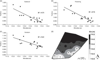
, Eq. 7) and the elevation of the field was calculated. For the field under consideration, the spatial component was strongly related to the elevation of the field for all the phenological stages (Fig. 2 a,b and c), although there is only 2.5 meters of difference between the highest and lowest site of the field (Fig. 2 d). The relation between vector a and elevation reflects the high stability of vector a, since the topography corresponds to a factor that does not change with the time. This is associated with the high stability of the spatial variability of phenology observed in this field (Verdugo-Vásquez et al., Reference Verdugo-Vásquez, Acevedo-Opazo, Valdés-Gómez, Araya-Alman, Ingram, García de Cortázar-Atauri and Tisseyre2015a). In the future, this relationship between the spatial component and the elevation of the field would allow the implementation of a fast and easy-to-start spatio-temporal model, where only climate information and field topography are needed to generate maps of the key phenological stages, considering the spatial variability of the field.
Relationship between vector a of the spatial model and the elevation of the field, for each phenological stage. a) Budburst, b) Flowering and c) Veraison. d) Field elevation (Ele).

Conclusion
This study showed that collaboration between a classical model of phenology based on climate data and a spatial model calibrated with ancillary data of phenology observations may improve the estimation of key phenological stages at the within field scale compared to when only the temporal model is considered. This work offers great promises to improve the calibration of a site-specific phenology model in grapevines. Indeed future research should focus on improving the link between temporal and spatial part of the model as well as estimating the spatial component using auxiliary information like elevation.
Acknowledgements
The authors of this paper wish to thank National CONICYT Doctoral Fellowship 2013N°21130504, FONDECYT Project 11110137 and PIEI Program of Agricultural Adaptation to Climate Change funded by the University of Talca.