

1. Introduction
This paper aims at analyzing the output multiplier associated with different tax-financing methods in the open economy. The Great Recession has revived interests in fiscal policy over business cycles. Diverse channels of output multiplier of government spending, such as a zero lower bound constraint, nominal price rigidities, and diverse fiscal rules to overcome negative wealth effects on private consumption in a representative agent New Keynesian (RANK) model have been extensively explored. Christiano et al. (Reference Christiano, Eichenbaum and Rebelo2011) and Woodford (Reference Woodford2011) show that the government spending multiplier can be larger at the zero lower bound in a RANK model, while Monacelli and Perotti (Reference Monacelli and Perotti2011) emphasize the redistribution channel for the size of fiscal multiplier in a two-agent New Keynesian (TANK) model.
As financial frictions in the form of borrowing constraints are increasingly relevant during and in aftermath of financial crisis, it warrants to analyze the effect of fiscal stimulus employing a tractable two-agent model. This paper deals with a largely overlooked redistribution channel of fiscal policy in open economies with borrowing constraints. For this purpose, we set up a simple two-agent small open economy with flexible prices as in Monacelli and Perotti (Reference Monacelli and Perotti2011) and address whether and how the fiscal expansion with different tax financing rules affects the output and aggregate consumption multiplier in the open economy. We abstract from any monetary frictions by assuming that prices are fully flexible as in Benigno and de Paoli (Reference Benigno and de Paoli2010) and Jung (Reference Jung2025) and leave aside the discussion of the implications associated with the extended model with nominal price rigidities in the appendix.
Monacelli and Perotti (Reference Monacelli and Perotti2011) show that the tax financing rule does not matter to the size of the government spending multiplier in the closed economy with flexible prices if savers and borrowers have the same steady-state consumption or inelastic labor supply. Otherwise, the tax financing rule matters. We will explore whether the so-called irrelevance of tax financing rules still holds in the open economy. Since the terms of trade variation critically depends on which category of households in the economy bears the brunt of tax hikes associated with a fiscal expansion, we need to explore how the interaction of the terms of trade and heterogeneity in households shapes the output multiplier under alternative tax financing rules. Specifically, we discuss how the terms of trade movements affect the government spending multiplier associated with alternative tax financing methods in the open economy.
Related literature
Early literature on the fiscal multiplier remains silent on the distribution channel which plays a prominent role in the recent discussion of monetary and fiscal policy in heterogeneous-agent New Keynesian (HANK) models as in Auclert (Reference Auclert2019), Kaplan et al. (Reference Kaplan, Moll and Violante2018), and Farhi and Werning (Reference Farhi, Werning, Taylor and Uhling2017). Since the HANK models require the use of nontrivial computational and numerical techniques to solve the equilibria for tracking of the distribution of wealth, many authors set up a simple and tractable alternative TANK model and discuss the redistribution channel of fiscal and monetary policy over business cycles (Bilbiie, Reference Bilbiie2008; Cúrdia and Woodford, Reference Cúrdia and Woodford2011; Eggertsson and Krugman, Reference Eggertsson and Krugman2012; Nisticó, Reference Nisticò2016). Galí et al., (Reference Galí, López-Saildo and Vallés2007), and Monacelli and Perotti (Reference Monacelli and Perotti2011), and Bilbiie et al. (Reference Bilbiie Florin, Monacelli and Perotti2013) analyze the fiscal multiplier in a closed economy TANK model, while Farhi and Werning (Reference Farhi, Werning, Taylor and Uhling2017) go one step further to explore fiscal multipliers in NK models with liquidity traps.
The main findings of this paper can be summarized as follows.
First, the tax-financing methods for government spending are relevant to resource allocations in a small open economy two- agent model with flexible prices, even if both unconstrained and constrained households have the same steady-state consumption, contrasting to the result of Monacelli and Perotti (Reference Monacelli and Perotti2011) in closed economies. Depending on which category of households bears the brunt of the necessary adjustment in taxations, the size of the terms of trade variation and the output multiplier to the government spending shock are different in open economy with flexible prices. Since each type of households is asymmetrically exposed to the financial risks, even if households have the so-called Cole and Obstfeld (Reference Cole and Obstfeld1991) preference wherein the financial structure is irrelevant to the resource allocations in the representative-agent economy model, the tax-financing rules feature a redistributive content. The tax-financing methods for fiscal expansion which generate a different path of the terms of trade always matter to the resource allocations and output multiplier in the two-agent open economy model with flexible prices.
Second, the output multiplier of the government spending in open economies with flexible prices is larger than the multiplier in closed economies with flexible prices when taxes are levied on constrained households, while the reverse is true when taxes are levied on unconstrained households. This stark result is closely linked to the different responses of labor supply and the real wage rate, which in turn depends on the terms of trade appreciation rate. When taxes are levied on constrained households, the terms of trade appreciates mildly, which in turn increases the real wage and labor hours in open economies. However, there occurs a small increase in labor hours with a muted change in the wage rate in closed economies, yielding a smaller output multiplier than in open economies. When taxes are levied on unconstrained households, there occurs a sharp terms of trade appreciation, inducing both domestic and foreign households to sharply divert their demand for goods toward foreign goods. Hence, the output multiplier under taxations on unconstrained households is smaller in open economies than in closed economies.
Finally, the output multiplier associated with taxes on constrained households is larger than the multiplier associated with taxes on unconstrained households in open economies with flexible prices,Footnote 1 irrespective of tax financing rules and debt limits. Taxations on unconstrained households which directly affect unconstrained households’ consumption and the international relative price through the risk-sharing condition generate a larger terms of trade appreciation than taxations on constrained households. Hence the demand for domestic goods contracts more under taxations on unconstrained households than under taxations on constrained households, yielding the smaller output multiplier under taxations on constrained households.
The remainder of the paper is organized as follows. Section 2 presents a small open economy model with unconstrained households and constrained households and section 3 presents equilibrium and some intuition of the effect of fiscal policy. Section 4 addresses the effect of government expenditure financing method on the fiscal multiplier, abstracting from monetary policy and section 5 concludes.
2. The model
This section sets up a variant of small open economy two-agent model with limited asset market participation applied to an open-economy. The world is composed of two countries, home
 $(H)$
and foreign
 $(F)$
with population size
 $n$
and
 $1-n$
respectively. It is assumed that the relative size of domestic economy is negligible relative to the rest of the world, i.e.
 $n\longrightarrow 0.$
A share of
 $1-\lambda$
of the continuum of households—referred to as unconstrained households—have access to financial markets, while the remaining share
 $\lambda$
of the households—referred to as constrained households—do partially trade assets. The model closely follows the flexible-price version of the small open economy two-agent model à la Galí and Monacelli (Reference Galí and Monacelli2005).
2.1 Households
There is a continuum of households
 $i\in \lbrack 0,1],$
all having the same utility function
 $u(C_{i,t},N_{i,t})=\ln (C_{i,t})-\omega _{i}\frac {N_{i,t}^{1+\nu }}{1+\nu }.$
In this paper, we assume that there are two types of households,
 $i=R,K.$
A
 $1-\lambda$
share is unconstrained household who holds all the shares in domestic firms with discount factor
 $\beta _{R}$
and the remaining
 $\lambda$
is constrained household share is constrained household with discount factor
 $\beta _{K}\lt \beta _{R}.$
Households also differ in their preference for leisure
 $\omega _{i}.$
2.1.1 Unconstrained households
Unconstrained households who can have access to financial markets choose their consumption, asset holdings, and labor supply, solving the standard intertemporal problem:
 \begin{equation*} \max .E_{t}\left [ \sum _{i=0}^{\infty }\beta _{R}^{i}u(C_{R,t+i},N_{R,t+i}) \right ] ,\,\,0\lt \beta _{R}\lt 1, \end{equation*}
subject to the sequence of budget constraints
 \begin{eqnarray} &&C_{R,t}+A_{R,t+1}+\Omega _{t+1}V_{R,t}+P_{t}^{-1}E_{t}[Q_{t,t+1}\mathcal{B} _{R,t+1}] \\ &=&P_{t}^{-1}\mathcal{B}_{R,t}+R_{t-1}A_{R,t}+\Omega _{R,t}(V_{R,t}+\mathcal{ P}_{R,t})+W_{t}N_{R,t}-T_{R,t}, \nonumber \end{eqnarray}
where
 $E_{t}$
denotes the expectations operator,
 $C_{R,t}$
and
 $N_{R,t}$
represent unconstrained household’s consumption and working hours in period
 $ t,$
respectively.
Here
 $A_{R,t},$
 $\Omega _{R,t},$
 $V_{R,t},$
and
 $\mathcal{P}_{R,t}$
denote the real value of domestic private assets, the share holdings, the real market value of shares in domestic goods-producing firms, and the corresponding real dividend payoffs at time
 $t,$
respectively.
 $T_{R,t},\ R_t,$
and
 $ W_{t}$
denote the lump-sum transfer/tax to the unconstrained households, the real interest rate and the real wage, respectively.
 $\mathcal{B}_{R,t+1}$
is the one-period nominal state-contingent home-currency bond purchased in period
 $t$
and
 $Q_{t,t+1}$
is the corresponding stochastic discount factor in period
 $t.$
Here
 $C_{R,t}$
is a composite consumption index defined by
 \begin{equation*} C_{R,t}=\left[(1-\gamma )^{\frac {1}{\eta }}C_{R_{H,}t}{}^{\frac {\eta -1}{\eta } }+\gamma ^{\frac {1}{\eta }}C_{R_{F,}t}{}^{\frac {\eta -1}{\eta }}\right]^{\frac { \eta }{\eta -1}},\;\eta \gt 0, \end{equation*}
where
 $\gamma \equiv \theta (1-n)$
and
 $C_{R_{H,}t}$
and
 $C_{R_{F,}t}$
are indices of domestic and foreign consumption goods consumed by domestic unconstrained households and
 $1-\theta$
and
 $\theta$
represent the share of domestic consumption allocated to domestic goods, and imported goods. As
 $ n\rightarrow 0$
in the small open economy
 $,$
it follows that
 $\gamma =\theta .$
The indices are given by the following CES aggregator of the quantities consumed of each variety of good:
 \begin{equation*} C_{R_{H,}t}=\left[\int _{0}^{1}C_{R_{H,}t}(z)^{\frac {\epsilon -1}{\epsilon }}dz\right]^{ \frac {\epsilon }{\epsilon -1}},\,\,\,C_{R_{F},t}=\left[ \int _{0}^{1}C_{R_{F},t}(z)^{\frac {\epsilon -1}{\epsilon }}dz\right]^{\frac { \epsilon }{\epsilon -1}},\,\,\,\,\epsilon \gt 1. \end{equation*}
Here
 $\eta$
and
 $\epsilon$
measure the elasticity of substitution between domestic and foreign goods, and the elasticity of substitution among goods within each category. The consumer price index (CPI)
 $P_{t}$
is given by
 $ P_{t}\equiv \lbrack \left ( 1-\alpha \right ) P_{H,t}^{1-\eta }+\alpha P_{F,t}^{1-\eta }]^{\frac {1}{1-\eta }}$
and
 $\pi _{t}\equiv \frac { P_{t}-P_{t-1}}{P_{t-1}}$
is the CPI inflation rate. The domestic goods price and import goods price indices
 $P_{H,t}$
and
 $P_{F,t}$
are given by
 $P_{H,t}= \left [ \int _{0}^{1}P_{H,t}(z)^{1-\epsilon }dz\right ] ^{\frac {1}{1-\epsilon } },\ \ P_{F,t}=\left [ \int _{0}^{1}P_{F,t}(z)^{1-\epsilon }dz\right ] ^{\frac {1 }{1-\epsilon }}.$
The intratemporal condition and the Euler equation for private assets and shareholdings respectively are given by
 \begin{align}&\qquad\qquad\quad \omega _{R}C_{R,t}N_{R,t}^{\nu }=W_{t}, \end{align}
 \begin{align}&\qquad\quad \beta E_{t}\left[\left(\frac {C_{R,t+1}}{C_{R,t}}\right)^{-1}R_{t}\right]=1, \end{align}
 \begin{align}& \beta E_{t}\left[\left(\frac {C_{R,t+1}}{C_{R,t}}\right)^{-1}\left(\frac {V_{R,t+1}+\mathcal{P}_{t} }{V_{R,t}}\right)\right]=1. \end{align}
The optimal risk-sharing condition between domestic unconstrained households and households in the rest of the world implies
 \begin{equation} \mathcal{Q}_{t}\equiv \frac {\mathcal{E}_{t}P_{t}^{\ast }}{P_{t}}=\left ( \frac {C_{t}^{\ast }}{C_{R,t}}\right ) ^{-1}, \end{equation}
where
 $\mathcal{E}_{t}$
and
 $\mathcal{Q}_{t}$
are the nominal and real exchange rate at time
 $t$
, respectively. Substituting the CPI index into (5) leads to the relationship between the relative consumption ratio and the terms of trade
 $\mathcal{S}_{t}(\equiv \frac {P_{F,t}}{P_{H,t}})$
as follows
 \begin{equation} \left ( \frac {C_{R,t}}{C_{t}^{\ast }}\right ) =\mathcal{S}_{t}[\left ( 1-\theta \right ) +\theta \mathcal{S}_{t}^{1-\eta }]^{\frac {1}{\eta -1}}\equiv \mathcal{H}(\mathcal{S}_{t}). \end{equation}
(6) shows that consumption of constrained households who lack access to the international financial market does not matter to the international relative price.
2.1.2 Constrained households
Assume that domestic constrained households can only borrow from domestic unconstrained households up to a limit of
 $\overline {A}.$
Constrained household’s budget constraint can be specified as follows:
 \begin{equation} C_{K,t}+A_{K,t+1}=R_{t}A_{K,t}+W_{t}N_{K,t}-T_{K,t} \end{equation}
and a borrowing constraint
 \begin{equation} -A_{K,t+1}\leq \overline {A}. \end{equation}
If
 $\overline {A}=0,$
then constrained households cannot have access to the financial market at all.
 \begin{equation*} C_{K,t}=W_{t}N_{K,t}-T_{K,t}, \end{equation*}
where
 $T_{K,t}$
is the lump-sum tax or transfer to constrained households in period
 $t$
.
Constrained household’s optimization conditions are given by
 \begin{align}&\qquad \omega _{K}N_{K,t}^{\nu }{}C{}_{K,t}=W_{t}, \end{align}
 \begin{align}& C{}_{K,t}^{-1}=\beta _{K}E_{t}\left [ R_{t}C{}_{K,t+1}^{-1}\right ] +\psi _{t}, \end{align}
and the budget constraint (7) and the borrowing constraint (8).
 $\psi _{t}$
is the Lagrange multiplier associated with the budget constraint and borrowing constraint, respectively.
2.2 Domestic firms
Differentiated goods and monopolistic competition are introduced along the lines of Dixit and Stiglitz (Reference Dixit and Stiglitz1977). Suppose that there is a continuum of firms producing differentiated goods, and each firm indexed by
 $z\in \lbrack 0,1]$
produces its product with a linear technology
 $Y_{t}(z)=N_{t}(z)$
.
Since the input markets are perfectly competitive, the firm
 $z^{\prime }$
s demand for labor is determined by its cost minimization as
 $W_{t}=\frac { MC_{r,t}}{(1-\tau _{n})}\frac {P_{H,t}}{P_{t}}.$
Here
 $MC_{r,t}\equiv \frac { MC_{t}}{P_{H,t}}$
is a domestic firm’s real marginal cost and
 $MC_{t}$
is the corresponding nominal marginal cost in period
 $t.$
Along the line of Benigno and de Paoli (Reference Benigno and de Paoli2010), Jung (Reference Jung2025), and Monacelli and Perotti (Reference Monacelli and Perotti2011), the monopolistically competitive firms in the domestic product markets set their own price by maximizing the present discounted value of profits. The firm
 $z$
’s maximization problem can be written as follows:
 \begin{equation*} \max .\;\frac {\Lambda _{t}}{P_{t}}[P_{H,t}(z)Y_{t}(z)-(1-\tau _{n})P_{t}W_{t}N_{t}(z)]\} \end{equation*}
subject to
 \begin{equation*} Y_{t}(z)\leq \left ( \frac {P_{H,t}(z)}{P_{H,t}}\right ) ^{-\epsilon }Y_{t}, \end{equation*}
where
 $\Lambda_{t}$
is the marginal utility of consumption of unconstrained household.
 $Y_{t}$
is the aggregate world demand for domestic products in period
 $ t$
and
 $\tau _{n}$
is employment subsidy to restore the marginal cost pricing in the steady state as in Benigno and de Paoli (Reference Benigno and de Paoli2010) and Jung (Reference Jung2025).
Since the optimal price setting is identical, the newly determined prices at time
 $t$
is given by
 \begin{equation} \frac {P_{H,t}}{P_{t}}=\frac {(\epsilon -1)W_{t}}{\epsilon (1-\tau _{n})}. \end{equation}
The CPI index implies that
 $\frac {P_{t}}{P_{H,t}}=[\left ( 1-\alpha \right ) +\alpha \mathcal{S}_{t}^{1-\eta }]^{\frac {1}{1-\eta }}\equiv \mathcal{K}( \mathcal{S}_{t})$
. Hence, (11) can be expressed in terms of
 $ \mathcal{S}_{t}$
:
 \begin{equation} W_{t}=\frac {\mathcal{MC}}{(1-\tau _{n})\mathcal{K}(\mathcal{S}_{t})}, \end{equation}
where
 $\mathcal{MC\equiv }\frac {(\epsilon -1)}{\epsilon }$
is the domestic real marginal cost in the flexible price equilibrium. Note that the employment subsidy
 $\tau _{n}=\frac {1}{\epsilon -1}$
restores the marginal cost pricing comparable to the one in the perfectly competitive markets as in Bilbiie (Reference Bilbiie2008) and Benigno and de Paoli (Reference Benigno and de Paoli2010).Footnote
2
2.3 Importing firms
For the sake of simplicity, it is assumed that the Law of One Price holds:
 \begin{equation*} P_{F,t}(z)=\mathcal{E}_{t}P_{F,t}^{\ast }(z), \end{equation*}
where
 $P_{F,t}(z),$
 $P_{F,t}^{\ast }(z)$
denote the price of foreign good
 $z$
in domestic currency and its price denominated in foreign currency at time
 $t$
.
In the rest of the world, a representative household faces a problem identical to the one outlined above. The only difference is that a negligible weight is assigned to consumption goods produced in a small economy
 $(\theta ^{\ast }=1).$
Therefore,
 $P_{t}^{\ast }=P_{F,t}^{\ast }$
and
 $C_{t}^{\ast }=C_{F,t}^{\ast }$
for all
 $t.$
2.4 Government
The fiscal authority finances its spending through taxation on either unconstrained or constrained households. Hence the budget constraint is given by
 \begin{eqnarray} P_{H,t}G_{t} &=&P_{t}T_{t}, \\ \lambda T_{K,t} &=&\omega T_{t}, \nonumber \end{eqnarray}
where
 $T_{t}\equiv (1-\lambda )T_{R,t}+\lambda T_{K,t}$
and
 $\omega$
is the share of taxes levied on constrained households.
Assume that the government collects lump-sum taxes and then redistribute them across unconstrained households and constrained households as in Monacelli and Perotti (Reference Monacelli and Perotti2011). Furthermore, the (log) government spending,
 $ g_{t}(\equiv$
log
 $G_{t})$
is assumed to follow an AR(1) process as follows:
 \begin{equation} g_{t}=(1-\rho _{g})g+\rho _{g}g_{t-1}+\varepsilon _{g,t}, \end{equation}
where
 $\varepsilon _{g,t}$
is an i.i.d. innovation at time
 $t$
.
2.5 Aggregation
The aggregate level of any household-specific variable
 $X_{t}$
is given by
 $ X_{t}=\int _{0}^{1}X_{t}(i)di=(1-\lambda )X_{R,t}+\lambda X_{K,t}.$
Hence, aggregate consumption, hours, and dividend are given by
 \begin{eqnarray*} C_{t} &=&(1-\lambda )C_{R,t}+\lambda C_{K,t}, \\ N_{t} &=&(1-\lambda )N_{R,t}+\lambda N_{K,t}, \\ \mathcal{P}_{t} &=&(1-\lambda )\mathcal{P}_{R,t}, \end{eqnarray*}
where the aggregation of domestic firms’ profits is given by
 \begin{equation} \mathcal{P}_{t}=\frac {Y_{t}}{\mathcal{K}(\mathcal{S}_{t})}-(1-\tau _{n})w_{t}N_{t}. \end{equation}
Since private debt is in zero net supply,
 $\int _{0}^{1}A_{t}(i)di=0$
and households of a certain type make symmetric decision, aggregate private bond holdings satisfy
 \begin{equation} (1-\lambda )A_{R,t}+\lambda A_{K,t}=0. \end{equation}
3. Equilibrium
Equity market clearing condition implies that shareholdings of each unconstrained household equal, given by
 $\Omega _{R,t+1}=\Omega =\frac {1}{1-\lambda }.$
The unconstrained household’s budget constraint with
 $\overline {A}=0$
can be simplified as
 \begin{equation} C_{R,t}+E_{t}\left[\frac {Q_{t,t+1}}{P_{t}}\mathcal{B}_{R,t+1}\right]=\frac {\mathcal{B} _{R,t}}{P_{t}}+\frac {1}{1-\lambda }\mathcal{P}_{t}+W_{t}N_{R,t}+\frac { \lambda }{(1-\lambda )}T_{K,t}-\frac {1}{(1-\lambda )\mathcal{K}(\mathcal{S} _{t})}G_{t}. \end{equation}
Equation (17) shows that taxation matters through taxation or transfer effect on constrained households in unconstrained households's budget constraint. Since unconstrained households hold assets, they can internalize the taxation on themselves through the effect of tax or transfers to constrained households.
Assuming a symmetric degree of home bias across countries with the negligible relative size of home country, goods market clearing condition in home and foreign countries requires that
 \begin{equation} (1-\lambda )N_{R,t}+\lambda N_{K,t}=(1-\theta )\mathcal{K}(\mathcal{S} _{t})^{\eta }C_{t}+\theta \mathcal{S}_{t}^{\eta }C_{t}^{\ast }+G_{t}, \end{equation}
 \begin{equation*} Y_{t}^{\ast }=C_{t}^{\ast }. \end{equation*}
(5) and (18) also imply that net exports can be expressed in terms of consumption heterogeneity and the terms of trade in a two-agent open economy model. For the sake of simplicity, consider net exports with a Cole and Obstfeld (Reference Cole and Obstfeld1991) preference. Combining the optimal risk-sharing condition (5) and the domestic goods market clearing condition (18) for
 $\sigma =\eta =1$
, net exports can be expressed as
 \begin{equation} NX_{t}=\lambda \theta \mathcal{S}_{t}^{\theta }(C_{R,t}-C_{K,t}). \end{equation}
(19) shows that there occurs trade imbalance if there is consumption gap between unconstrained households and constrained households in open economies with a Cole-Obstfeld preference. There is trade surplus if
 $C_{R,t}\gt C_{K,t}$
. Otherwise, there is trade deficit.
We focus a symmetric equilibrium with flexible prices in which all firms in the same country set the same prices, i.e.
 $P_{H,t}(z)=P_{H,t},P_{F,t}(z)=P_{F,t}$
as in Benigno and de Paoli (Reference Benigno and de Paoli2010) and Jung (Reference Jung2025), abstracting from any monetary frictions. The symmetric competitive equilibrium conditions consist of the efficiency conditions and the budget constraint of the households and firms, and the market clearing conditions of each goods market, labor market, money, and bond market under each asset market regime.
Specifically, the symmetric equilibrium with flexible prices is a sequence of prices and quantities for home country
 $\{C_{R,t},N_{R,t},C_{K,t}, N_{K,t},W_{t},R_{t},\mathcal{P}_{t},V_{t},\mathcal{S}_{t},A_{R,t},A_{Kt}, \psi _{t}\}_{t=0}^{\infty }$
that satisfy (2), (3), ( 4), (6), (7), (8), ( 9), (10), (12), (15), (16), (18), and
 $\Omega _{R,t}=\Omega =\frac {1}{1-\lambda }$
for all time, given the foreign output and prices of the rest of the world
 $\{Y_{t},P_{t}^{\ast }\}_{t=0}^{\infty },$
and exogenous government spending shock process
 $\{G_{t}\}_{t=0}^{\infty }$
as well as the tax financing method policies
 $\{T_{R,t},T_{K,t}\}_{t=0}^{\infty }$
.
3.1 Steady state
In the steady state with
 $A_{K}=\overline {A}$
, (3) and (10) show that
 \begin{eqnarray*} R &=&\beta _{R}^{-1}, \\ \psi &=&C_{K}^{-1}\left(1-\frac {\beta _{K}}{\beta _{R}}\right). \end{eqnarray*}
For the sake of simplicity, we assume that constrained and unconstrained households work the same number of hours in the steady state, consistent with the view that there are no wealth effects on long-run labor hours as in Bilbiie at al. (Reference Bilbiie Florin, Monacelli and Perotti2013). The weights in utility
 $\omega _{R}$
and
 $\omega _{K}$
consistent with this assumption should satisfy
 \begin{equation*} \omega _{R}=\left ( 1+\frac {\lambda }{1+\lambda }r\delta _{B}\right ) ^{-1}\Theta _{i}\lt \omega _{K}=\left ( 1-r\delta _{B}\right ) ^{-1}N^{1+\nu }, \end{equation*}
where
 $\delta _{B}\equiv \frac {\overline {A}}{Y}\geq 0$
is the constrained household’s steady-state debt-to-income ratio.
The ratio of unconstrained household’s consumption relative to the aggregate consumption at the steady state is given by
 \begin{equation} \gamma \equiv \frac {C_{R}}{C}=\frac {1-\lambda \chi }{1-\lambda }\geq 1, \end{equation}
where
 $\chi \equiv \frac {C_{K}}{C}.$
3.2 Parameter values
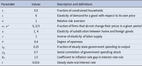
All parameter values used in this paper are reported in Table 1 which are taken from Galí and Monacelli (Reference Galí and Monacelli2005), Monacelli and Perotti (Reference Monacelli and Perotti2011), and Bilbiie et al., (Reference Bilbiie Florin, Monacelli and Perotti2013). First, the Frisch labor supply elasticity of labor supply, i.e.
 $\nu ^{-1}$
is set to 1 in the benchmark model. The intratemporal elasticity between home and foreign goods
 $\eta$
which plays a key role in the dynamic properties of the selected macroeconomic variables in the model is set to values in
 $[1,4]$
. The unconstrained household’s subjective discount factor is set to 1.04
 $^{-1/4},$
which is consistent with an annual real rate of interest of 4 percent as in the literature. Constrained household’s discount factor is set to 0.98 as in Monacelli and Perotti (Reference Monacelli and Perotti2011).
The calibrated parameters

The fraction of constrained households
 $\lambda$
is set to
 $0.5$
and the autoregressive parameter of government spending
 $\rho _{g}$
is set to 0.7 as in Monacelli and Perotti (Reference Monacelli and Perotti2011). Finally, the steady-state debt-to-income ratio
 $\delta _{B}$
is set values in
 $[0,0.8]$
.
4. Government spending and tax financing rules
In this section, we address how the tax burden affects the government spending multiplier in the small open economy two-agent model with flexible prices equilibrium in which fiscal authority sets an employment subsidy to restore the marginal cost pricing, i.e.,
 $\tau _{n}=\frac {1}{\epsilon }$
. Specifically, we discuss whether the tax financing method matters to the multiplier of fiscal policy under the assumption that there is no public debt.
To address the relevance of tax financing methods in the open economy with flexible prices, we first consider the benchmark along the line of Bilbiie (Reference Bilbiie2008) and Monacelli and Perotti (Reference Monacelli and Perotti2011) by assuming that debt-limit is zero
 $(\overline {A}=0),$
i.e.,
 $\delta _{B}=0,$
and then discuss the implications of the model by relaxing the assumption of
 $\delta _{B}=0$
. Under this assumption, the profit is zero and the ownership structure of firms are irrelevant. Both unconstrained and constrained households consume the same amount of goods in the steady state.
4.1 Relevance of taxation methods
To formally discuss how the degree of openness and the terms of trade externality matters to tax financing rules in the flexible price equilibrium, we will first present the conditions under which the irrelevance result of tax financing rule holds in closed economies (Monacelli and Perotti, Reference Monacelli and Perotti2011).
Lemma 1.
In the economy with flexible prices and constant returns to scale in production, if unconstrained and constrained households are equally taxed
 $ (\tau _{R,t}=\tau _{K,t})$
and the distribution is degenerate
 $(\overline {A}=0)$
at the deterministic steady state, then the tax financing rule is irrelevant. (Monacelli and Perotti, Reference Monacelli and Perotti2011).
To formally discuss the effect of the degree of openness and the terms of trade externality on the relevance of tax financing rule in the flexible price equilibrium, we need to express consumption and labor hours in log-linear deviation forms from the steady state. Using the resource constraint with borrower’s budget constraint (by Walras law), unconstrained and constrained household’s (log) consumption around the steady state can be expressed as follows:
 \begin{align}&\qquad c_{R,t}=\frac {\mathbf{S}_{c}^{\ast }}{\mathbf{S}_{c}}c_{t}^{\ast }-\frac { \theta s_{c}\lambda }{\left(s_{c}+\frac {1}{\nu }\right)\mathbf{S}_{c}}\tau _{K,t}-\frac { (1-\lambda )}{\mathbf{S}_{c}}\tau _{R,t}, \end{align}
 \begin{align}& c_{K,t}=-\mathbf{B}_{K}\tau _{K,t}+\mathbf{B}_{R}\tau _{R,t}+\theta \left(1+\frac { 1}{\nu }\right)\left(1-\frac {\mathbf{S}_{c}^{\ast }}{(1-\theta )\mathbf{S}_{c}} \right)c_{t}^{\ast }, \end{align}
where
 $s_{c}\equiv \frac {C}{Y}$
and
 \begin{eqnarray} \mathbf{S}_{c} &\equiv &\theta \left(\frac {\eta (2-\theta )}{1-\theta }+\frac { (1-\lambda )}{\nu (1-\theta )}+\frac {\lambda \left(1+\frac {1}{\nu }\right)s_{c}}{\left(s_{c}+ \frac {1}{\nu }\right)(1-\theta )}-\frac {1}{1-\theta }\right)+\frac {(1-\lambda )}{\nu } +(1-\theta )(1-\lambda )s_{c}, \nonumber \\ \mathbf{S}_{c}^{\ast } &\equiv &\theta \left(\frac {\eta (2-\theta )}{1-\theta }+ \frac {(1-\lambda )}{\nu (1-\theta )}+\frac {\theta \lambda \left(1+\frac {1}{\nu } \right)s_{c}}{\left(s_{c}+\frac {1}{\nu }\right)(1-\theta )}-\frac {1}{1-\theta }-s_{c}\right), \nonumber \\ \mathbf{B}_{K} &\equiv &\frac {1}{s_{c}\left(1+\frac {1}{\nu }\right)}\left(1-\frac {\theta ^{2}\left(1+\frac {1}{\nu }\right)s_{c}\lambda }{(1-\theta )\left(s_{c}+\frac {1}{\nu }\right) \mathbf{S}_{c}}\right),\ \mathbf{B}_{R}\equiv \frac {\theta \left(1+\frac {1}{\nu } \right)(1-\lambda )}{(1-\theta )\mathbf{S}_{c}}. \end{eqnarray}
Here a small letter denotes log-deviations of a variable from its steady-state value.
Equations (21)–(23) show how the goods market openness shapes constrained and unconstrained households’ consumption when government levies equal taxations to all households. In the open economy in which only unconstrained households who have access to international financial markets can optimally hedge risks with households in the rest of the world, constrained and unconstrained households are asymmetrically exposed to the risks associated with unexpected shocks. Since the real exchange rate is closely linked to consumption of unconstrained households through the risk sharing condition, the tax financing rules shape very different features of the terms of trade and consumption.
Lemma2 states that the asymmetric exposure of constrained and unconstrained households to the risks makes the financing method for the government expenditure matter in the small open economy augmented with flexible prices, constant returns to scale (CRS) production function, and equally taxed agents in the steady state. This result contrasts with Monacelli and Perotti’s irrelevance result in the closed economies.
Lemma 2. In the two-agent small open economy with flexible prices and constant returns to scale in production, the tax financing method is relevant even if both agents are equally taxed in the steady state.
If the economy is closed, i.e., if
 $\theta =0,$
then
 $\mathbf{S} _{c}=(1-\lambda )s_{c}(1+\frac {1}{\nu })$
and
 $\mathbf{S}_{c}^{\ast }=0,$
implying that equations (21) and (22) boil down to Lemma1 of Monacelli and Perotti (Reference Monacelli and Perotti2011):
 \begin{align}& c_{R,t}=-\frac {\tau _{R,t}}{s_{c}+\frac {1}{\nu }}, \end{align}
 \begin{align}& c_{K,t}=-\frac {\tau _{K,t}}{s_{c}+\frac {1}{\nu }}. \end{align}
Equations (24) and (25) show that tax financing rule is irrelevant in the closed economy with flexible prices, i.e., for
 $\theta =0$
as in Monacelli and Perotti (Reference Monacelli and Perotti2011)
 $.$
It does not matter who pays the tax for government to spend an extra resource.
However, if the economy is open
 $(\theta \gt 0)$
, (21) and (22) show that the effect of fiscal policy on the economy is different, depending on taxation to specific groups. Contrary to the closed economy with flexible prices, the real wage is not time-invariant in the open economy with the flexible prices as the terms of trade fluctuations affect the consumer price index. Moreover, a fiscal expansion entails different dynamics of the terms of trade, depending on financing methods. Under flexible prices, (12) implies that
 $w_{t}=-\theta s_{t}.$
The size of a terms of trade appreciation and the increase of the real wage rate as well as labor hours depend on who bears the brunt of tax hikes. The real wage associated with taxation on unconstrained households is higher than the real wage associated with taxation on constrained households, yielding different labor hours of household in each group to the government spending shock.
Having discussed the relevance of taxation rules in the open economy, we will next study how the size of multiplier of government spending depends on the assumed tax financing methods. Specifically, we address how households in each group respond to a government spending shock under alternative tax financing rules.
4.2 Taxation on constrained households
Suppose that the fiscal authority finances an increased government expenditure by taxations on constrained households, i.e.,
 $\omega =1$
. To discuss how taxes levied on constrained households affect unconstrained households who internalize the taxation on constrained households, rewrite the unconstrained households’ consumption and labor hours in terms of the real wage, terms of trade, and taxation as follows:
 \begin{align}&\qquad\,\, n_{R,t}=\mathbf{A}_{w}w_{t}+\mathbf{A}_{s}s_{t}+\mathbf{A}_{\tau }\tau _{K,t}+\mathbf{A}_{c^{\ast }}c_{t}^{\ast }, \end{align}
 \begin{align}& c_{R,t}=(1-\nu \mathbf{A}_{w})w_{t}-\nu \mathbf{A}_{s}s_{t}-\nu \mathbf{A} _{\tau }\tau _{K,t}-\nu \mathbf{A}_{c^{\ast }}c_{t}^{\ast }. \end{align}
where
 \begin{eqnarray*} \mathbf{A}_{w} &\equiv &\frac {(1+\nu s_{K})[(1-\theta )(1-\lambda )s_{R}+\lambda (1-\theta )]-(1+s_{K})\lambda \theta }{(1-\lambda )(1+(1-\theta )\nu s_{R})(1+\nu s_{K})}, \\ \mathbf{A}_{s} &\equiv &\frac {\theta (\eta (2-\theta )s_{c}-s_{g})}{ (1-\lambda )(1+(1-\theta )\nu s_{R})}, \\ \mathbf{A}_{\tau } &\equiv &\frac {s_{g}\theta (2+\nu s_{K})}{(1-\lambda )(1+(1-\theta )\nu s_{R})(1+\nu s_{K})}, \\ \mathbf{A}_{c^{\ast }} &\equiv &\frac {\theta s_{c}}{(1-\lambda )(1+(1-\theta )\nu s_{R})}. \end{eqnarray*}
Here
 $s_{R}\equiv \frac {C_{R}}{Y},\ s_{K}\equiv \frac {C_{K}}{Y},$
and
 $ s_{g}\equiv \frac {G}{Y}$
denote the share of unconstrained and constrained household’s consumption, and government spending relative to output in the steady state, respectively. First, note that in the case of the closed economy
 $(\theta =0)$
with flexible prices, the markup or the real marginal cost is constant, implying that
 $w_{t}=\ln (\frac {P_{t}}{MC_{t}/(1-\tau _{n})})=0,$
and
 $n_{R,t}=c_{R,t}=0$
. Hence, taxations on constrained households do not affect unconstrained household’s consumption and labor hours in the closed economy with perfect competition in goods and labor markets if production functions feature CRS. Since the real wage is time-invariant in the closed economy with flexible prices and CRS production function, both consumption and labor hours of unconstrained households are time-invariant when taxes are levied on constrained households as in Monacelli and Perotti (Reference Monacelli and Perotti2011).
The effect of goods market openness on the multiplier of the government spending can be inspected through the lens of a terms of trade effect on consumption. Notice that under the flexible price equilibrium, the domestic real marginal cost is time-invariant, implying that
 $w_{t}=-\theta s_{t}.$
The real wage rate inversely varies with the terms of trade in open economies with flexible prices: The real wage rate in the open economy with flexible prices increases (decreases) if the terms of trade appreciates (depreciates). That is, in the open economy
 $(\theta \gt 0),$
domestic goods prices go up to the positive government spending shock when the fiscal authority increases its demand for domestic goods. Rearranging (27) after substituting the risk-sharing condition
 $c_{R,t}-c_{t}^{\ast }=(1-\theta )s_{t}$
and
 $w_{t}=-\theta s_{t}$
into (27) yields the terms of trade in terms of exogenous variables
 $\tau _{K,t}$
and
 $ c_{t}^{\ast }$
:
 \begin{equation} s_{t}=\frac {1}{1-\theta +\theta (1-\nu \mathbf{A}_{w})+\nu \mathbf{A}_{s}} \left[-\nu \mathbf{A}_{\tau }\tau _{K,t}+(1-\nu \mathbf{A}_{c^{\ast }})c_{t}^{\ast }\right]. \end{equation}
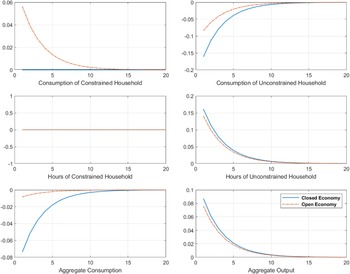
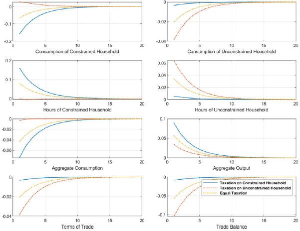
(28) shows that the terms of trade appreciates to the taxations on constrained households. Hence, consumption of unconstrained households decreases to the shock through the risk-sharing condition. Overall, the aggregate consumption decreases more in open economies than in closed economies when taxes are increased to constrained households. Figure 1 displays the impulse response of the domestic output to the government spending increase in closed and open economies for
 $\delta _{B}=0$
and
 $ \sigma =\eta =1$
in which the asset market structure is irrelevant to resource allocations and the monetary policy design for the representative-agent small open economy is isomorphic to the problem of the closed economy and openness does not affect the quantitative implications (Clarida et al., Reference Clarida, Galí and Gertler2001).
Impulse response function to government spending shock: taxataions on constrained households
 $(\delta _{B}=0, \eta =1)$
.

The effect of the market openness on the output multiplier of government spending can be inspected by analyzing the labor hours of unconstrained households. Substituting
 $w_{t}=-\theta s_{t}$
into (2) produces
 \begin{equation} \nu n_{R,t}=-c_{R,t}-\theta s_{t}. \end{equation}
(29) shows that unconstrained households expand their labor hours to taxations on constrained households in open economies, since the real wage rate increases with the terms of trade appreciation to the government spending shock. This contrasts to time-invariant labor hours of unconstrained households in closed economies. Turning to constrained households’ response to the shock, constrained households who lack access to international financial markets are exposed to financial risks and must expand their labor hours more sharply when taxes are levied on themselves. The expansion of labor hours of both constrained and unconstrained households reflects the stark difference between the output multiplier in open economies and the multiplier in closed economies when taxes are increased to constrained households. Figure 1 displays that there is trade surplus as in (19), since constrained households who lack access to financial markets also decrease their consumption more than unconstrained households who can have access to financial markets.
4.3 Taxation on unconstrained households
Next, consider the case of the government spending increase with taxations on unconstrained households, i.e.
 $\omega =0$
.
Taxations on unconstrained households induce constrained households to supply constant labor hours, irrespective of the market openness
 $(\theta )$
:
 \begin{equation*} n_{K,t}=0. \end{equation*}
Also, notice that
 \begin{align}&\qquad\qquad\qquad n_{R,t}=\mathbf{B}_{w}w_{t}+\mathbf{B}_{s}s_{t}+\mathbf{B}_{\tau }\tau _{R,t}+\mathbf{B}_{c^{\ast }}c_{t}^{\ast }, \end{align}
 \begin{align}& c_{R,t}=(1-\nu \mathbf{B}_{w})s_{R}^{-1}w_{t}-s_{R}^{-1}\nu \mathbf{B} _{s}s_{t}-s_{R}^{-1}(\nu \mathbf{B}_{\tau }+s_{\tau ,R})\tau _{R,t}-s_{R}^{-1}\nu \mathbf{B}_{c^{\ast }}c_{t}^{\ast }. \end{align}
where
 \begin{eqnarray*} \mathbf{B}_{w} &\equiv &\frac {(1-\theta )s_{c}[(1-\lambda \chi )s_{R}^{-1}+\lambda \chi ]}{(1-\lambda )[1+(1-\theta )(1-\lambda \chi )\frac { s_{s}\nu }{s_{R}}]}, \\ \mathbf{B}_{s} &\equiv &\frac {\theta \lbrack \eta (2-\theta )s_{c}+s_{g}]}{ (1-\lambda )[1+(1-\theta )(1-\lambda \chi )\frac {s_{s}\nu }{s_{R}}]}, \\ \mathbf{B}_{\tau } &\equiv &\frac {[s_{g}+(1-\theta )(1-\lambda \chi )\frac { s_{c}}{s_{R}}s_{\tau ,R}]}{(1-\lambda )[1+(1-\theta )(1-\lambda \chi )\frac { s_{s}\nu }{s_{R}}]}, \\ \mathbf{B}_{c^{\ast }} &\equiv &\frac {\theta s_{s}}{(1-\lambda )[1+(1-\theta )(1-\lambda \chi )\frac {s_{s}\nu }{s_{R}}]}. \end{eqnarray*}
As in previous subsection, rearranging (31) after substituting the risk-sharing condition
 $c_{R,t}-c_{t}^{\ast }=(1-\theta )s_{t}$
and
 $ w_{t}=-\theta s_{t}$
into (31) produces the terms of trade in terms of exogenous variables
 $\tau _{K,t}$
and
 $c_{t}^{\ast }$
:
 \begin{equation} s_{t}=\frac {1}{s_{R}(1-\theta )+(\theta (1-\nu \mathbf{B}_{w})+\nu \mathbf{B} _{s})}[(\nu \mathbf{B}_{\tau }+s_{\tau ,R})\tau _{R,t}+(s_{R}-\nu \mathbf{B} _{c^{\ast }})c_{t}^{\ast }]. \end{equation}
To inspect how constrained households adjust their labor hours to the government spending increases associated with taxations on unconstrained households, substitute
 $w_{t}=-\theta s_{t}$
into (9), which yields
 \begin{equation} c_{K,t}=-\nu n_{K,t}-\theta s_{t}. \end{equation}
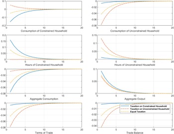
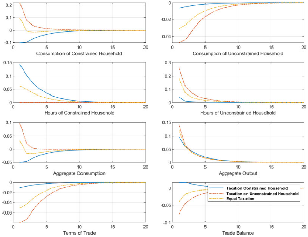
(33) shows that while labor hours of constrained households are time-invariant under taxations on unconstrained households, consumption of constrained households expands to the government shock in open economies as the real wage rate increases with the terms of trade appreciation. Hence, the aggregate consumption decreases less in open economies than in closed economies when taxes are increased to unconstrained households as in Figure 2. However, the large terms of trade appreciation associated with taxations on unconstrained households sharply diverts the demand for domestic goods toward foreign goods, yielding a smaller output expansion in open economies than in closed economies as in Figure 2.
Impulse response function to government spending shock: taxataions on unconstrained households
 $(\delta _{B}=0, \eta =1)$
.

Impulse response function to government spending shock
 $(\delta _{B}=0, \eta =1)$
.

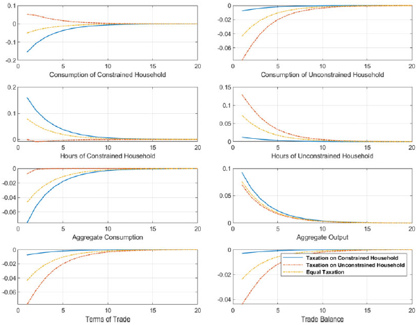
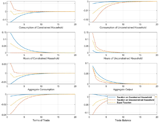
Finally, Figure 3 displays the dynamics of some selected variables to the government spending increases associated with alternative taxations in open economies for a Cole-Obstfeld preference
 $(\sigma =\eta =1)$
and
 $\delta _{B}=0$
: Taxations on constrained households, taxations on unconstrained households, and equal taxations on constrained and unconstrained households. Since the real exchange rate is proportional to unconstrained household’s consumption relative to foreign household’s consumption in open economies through the risk-sharing condition, taxations on unconstrained households generates a larger terms of trade appreciation than taxations on constrained households as in Figure 3. Consumption of unconstrained households barely reacts, but unconstrained households’ consumption substantially falls when taxes are increased to unconstrained households. Since taxations on constrained households generate a milder expenditure switching effects than any other tax financing rules, output expands more sharply when taxes are levied on constrained households relative to the case in which taxes are increased to unconstrained households.
Turning to the aggregate consumption multiplier, there occurs a reversal, since the purchasing power is improved most on taxations on unconstrained households, while it is improved least on taxations on constrained households as in Figure 3. The terms of trade is appreciated by less when households are equally taxed as opposed to the case when taxes are levied on unconstrained households only, but it is appreciated more sharply compared to the case when taxes are increased only to constrained households. Hence, the multiplier of output and aggregate consumption to the government spending shock associated with equal taxations is in the middle between the multiplier with taxations on constrained households and the multiplier with taxations on unconstrained households. Figure 3 shows that there occurs trade surplus for taxations on constrained households, while there occurs trade deficit for taxations on unconstrained households.
4.4 Sensitivity analysis
In this subsection, we will address how the deep parameters such as the intratemporal elasticity of substitution between home and foreign goods
 $ \eta$
and the steady-state debt-to-income ratio
 $\delta _{B}$
affect the ranking of the output and aggregate consumption multipliers under alternative tax financing methods. We also discuss how sensitive the output multiplier to the composition of tax adjustment, varying
 $\omega$
in (13).
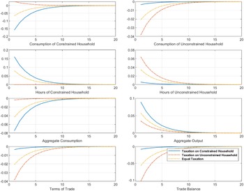
Impulse response function to government spending shock
 $(\delta _{B}=0, \eta =3)$
.

First, consider how the intratemporal elasticity of substitution between home and foreign goods shapes the output multiplier of government spending under alternative tax-financing rules. Figure 4 present the impulse response of some selected variables to the government spending increase under alternative tax finance rules for a high intratemporal elasticity of substitution between home and foreign goods
 $\eta =3$
. (28) and 32) show that the larger the intratemporal elasticity of substitution between home and foreign goods
 $\eta ,$
the smaller the appreciation of the terms of trade to the government spending increase, since
 $\mathbf{A}_{s}$
and
 $\mathbf{B}_{s}$
increase with
 $\eta .$
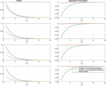
Hence, there occurs a smaller expansion of output and contraction of aggregate consumption to the government shock in economies with a high intratemporal elasticity of substitution than a low intratemporal elasticity of substitution, irrespective of tax financing rules. Comparison of Figure 3 and 4 shows that unconstrained households increase their labor hours less to the government spending increase in the economy with a high intratemporal elasticity of substitution compared to the case of a low intratemporal elasticity of substitution, since a milder terms of trade appreciation yields a smaller increase in the real wage for a high intratemporal elasticity of substitution. The high intratemporal elasticity of substitution between home and foreign goods dampens the output multiplier to the government spending shock, irrespective of tax financing rules.
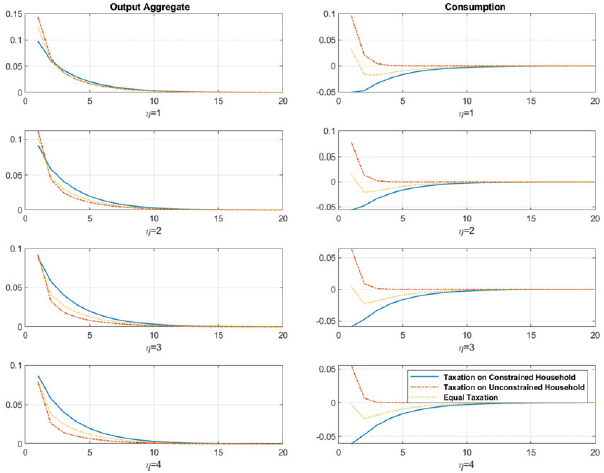
Impluse response function of output and aggregate consumption to government spending shock
 $(\delta _{B}=0)$
.

Figure 5 displays the output and aggregate consumption multiplier to the government spending increase under alternative tax financing rules in the economies with
 $\delta _{B}=0$
, varying the intratemporal elasticity of substitution between home and foreign goods
 $\eta$
from 1 to 4. Figure 5 confirms that the output multiplier dampens with the intratemporal elasticity substitution between home and foreign goods, but it does not change the ranking of the multipliers under alternative tax financing rules.
Impluse response function of output and aggregate consumption to government spending shock
 $(\eta =1)$
.

Impluse response function of output and aggregate consumption to government spending shock
 $(\eta =3)$
.

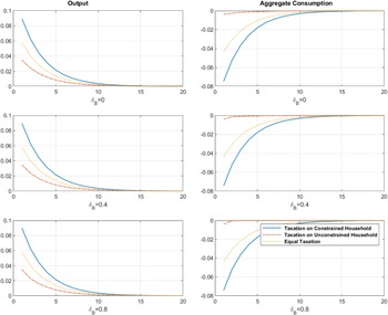
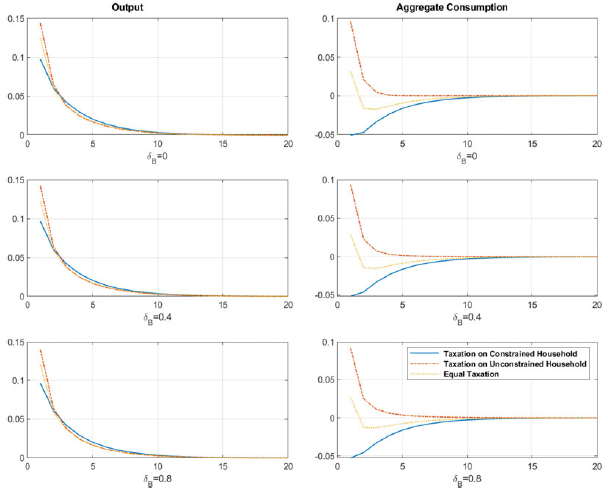
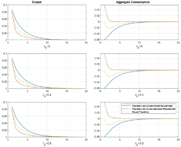
Figure 6 and 7 present the impulse response of the multiplier of output and aggregate consumption to the government spending shock under alternative tax financing rules for
 $\eta =1$
and
 $3$
, varying debt-limits
 $\delta _{B}$
. Though the debt-limit affects the steady-state consumption of each type of household, the quantitative effect of changing the borrowing constraint is marginal, irrespective of tax financing rules.Footnote
3
The figures also show that the steady-state debt-to-income ratio does not change the ranking of the output and aggregate consumption multiplier to the government spending, irrespective of tax financing rules. However, there occurs a larger gap between the output multiplier associated with taxations on constrained households and the multiplier with taxations on unconstrained households. The higher the intratemporal elasticity of substitution between home and foreign goods, the higher the expenditure switching effect to a given terms of trade variation. For a higher intratemporal elasticity of substitution, taxations on unconstrained households generate a larger crowding out effect in output.
Impulse response function to government spending shock
 $(\delta _{B}=0, \eta =1)$
.

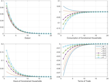
Finally, Figure 8 presents the response of output, terms of trade, and consumption and labor hours of constrained households to the government spending shock, varying the share of taxes levied on constrained households
 $ \omega$
for
 $\eta =1$
and
 $\delta _{B}=0.$
The figure shows that the larger the share of taxes levied on constrained households, the larger the burden of constrained households and the smaller the terms of trade appreciation. Constrained households with a larger tax burden work more hours to minimize the impact of taxations on their consumption. For a share of constrained households’ taxes equal to one, the output multiplier reaches a maximum value.
5. Conclusion
This paper sets up a small open economy model with constrained households and unconstrained households to address the effect of government spending associated with different financing methods.
This paper shows that tax financing rules are relevant in a small open economy with flexible prices and CRS production function, even if both unconstrained households and constrained households have the same steady-state consumption, contrasting with the findings of Bilbiie et al. (Reference Bilbiie Florin, Monacelli and Perotti2013) and Monacelli and Perotti (Reference Monacelli and Perotti2011) in the closed economy. There is no financial transaction in equilibrium in the closed economy with unconstrained and constrained households, while unconstrained households can lend or borrow by participating in the international financial market in the open economy. The paper also shows that the output multiplier of government spending associated with taxes on constrained households in open economies is larger than the multiplier in closed economies, while the reversal holds under taxations on unconstrained households. The paper also shows that the output multiplier of government spending associated with taxes on constrained households is larger than the one with taxes on unconstrained households.
Acknowledgement
I am grateful to two annoymous referees and the associate editor and to the seminar participants at the KDI, KIEP, KIPF, and Kyungpook University for helpful comments. All errors are my own.
Appendix A
A.1. Equal taxations
Consider first the budget constraints of each type household with debt-limits
 $\overline {A}=0$
.
 \begin{align*} C_{R,t}+E_{t}Q_{t,t+1}\mathcal{B}_{t}+\Omega _{t+1}V_{t}&=W_{t}N_{R,t}+\frac { \mathcal{B}_{t-1}}{1+\pi _{t}}+\Omega _{t}(V_{R,t}+\mathcal{P} _{R,t})-T_{R,t} \\ C_{K,t}&=W_{t}N_{K,t}-T_{K,t}, \end{align*}
where
 $T_{R,t}$
and
 $T_{K,t}$
are lump-sum taxation to unconstrained and constrained households at time
 $t$
.
Consider next the first-order conditions of unconstrained and constrained households and the goods market clearing condition,
 \begin{equation*} C_{R,t}N_{R,t}^{\nu }=\frac {\textrm{mc}}{1-\tau _{n}}\big[1-\theta +\mathcal{S} _{t}^{1-\eta }\big]^{\frac {-1}{1-\eta }}, \end{equation*}
 \begin{equation*} C_{K,t}N_{K,t}^{\nu }=\frac {\textrm{mc}}{1-\tau _{n}}\big[1-\theta +\mathcal{S} _{t}^{1-\eta }\big]^{\frac {-1}{1-\eta }}, \end{equation*}
 \begin{equation*} \big ( \frac {C_{R,t}}{C_{t}^{\ast }}\big ) =\mathcal{S}_{t}\left[1-\theta + \mathcal{S}_{t}^{1-\eta }\right]^{\frac {-1}{1-\eta }}, \end{equation*}
 \begin{equation*} C_{K,t}+T_{K,t}=\frac {\textrm{mc}}{1-\tau _{n}}\big[1-\theta +\mathcal{S} _{t}^{1-\eta }\big]^{\frac {-1}{1-\eta }}N_{K,t}, \end{equation*}
and
 \begin{equation*} Y_{t}-G_{t}=(1-\theta )\left((1-\theta )+\theta \mathcal{S}_{t}^{1-\eta }\right)^{\frac { \eta }{1-\eta }}((1-\lambda )C_{A,t}+\lambda C_{K,t})+\theta \mathcal{S} _{t}^{\eta }C_{t}^{\ast }. \end{equation*}
Log-linearization of the specified first-order conditions leads to
 \begin{align}&\qquad\qquad\qquad\qquad\qquad\qquad\quad\, c_{R,t}+\nu n_{R,t}+\theta s_{t}=0, \end{align}
 \begin{align}&\qquad\qquad\qquad\qquad\qquad\qquad s_{c}c_{K,t}+s_{g}\tau _{K,t}=-\theta s_{t}+n_{K,t} \end{align}
 \begin{align}&\qquad\qquad\qquad\qquad\qquad\qquad\quad c_{K,t}+\nu n_{K,t}+\theta s_{t}=0, \end{align}
 \begin{align}&\qquad\qquad\qquad\qquad\qquad\qquad\quad\,\, c_{R,t}-c_{t}^{\ast }=(1-\theta )s_{t}, \end{align}
 \begin{align}& ((1-\lambda )n_{A,t}+\lambda n_{K,t})-s_{g}g_{t}=\theta \eta (2-\theta )s_{t}+(1-\theta )s_{c}((1-\lambda )c_{A,t}+\lambda c_{K,t})+\theta s_{c}c_{t}^{\ast }, \end{align}
where
 $\tau _{i,t}\equiv \frac {T_{i,t}-T_{i}}{Y}$
for
 $i=R,K$
.
Suppose that government levies taxations
 $T_{R,t}$
and
 $T_{K,t}$
on unconstrained and constrained households.
 \begin{eqnarray*} T_{t} &=&(1-\lambda )T_{R,t}+\lambda T_{K,t}, \\ g_{t} &=&(1-\rho _{g})g+\rho _{g}g_{t-1}+\xi _{g,t}. \end{eqnarray*}
Then, (34) ∼(38) can determine
 $ \{c_{R,t},c_{K,t},n_{R,t},n_{K,t},s_{t}\}_{t=0}^{\infty }$
, given the exogenous variables
 $\{c_{t}^{\ast },g_{t},\tau _{R,t},\tau _{K,t}\}_{t=0}^{\infty }$
.Footnote
4
(35), (36), and the goods market clearing condition (38) yield
 \begin{align}&\qquad\qquad\qquad\qquad\qquad \left(s_{c}+\frac {1}{\nu }\right)c_{K,t}=-s_{g}\tau _{K,t}-\theta \left(1+\frac {1}{\nu } \right)s_{t}, \end{align}
 \begin{align}& (-(1-\lambda )(-\theta s_{t}-c_{K,t})\nu ^{-1}+\lambda n_{K,t})-s_{g}g_{t}=\theta \eta (2-\theta )s_{t}\nonumber\\&\qquad\qquad\qquad\qquad\qquad\qquad\qquad\qquad\qquad\quad +(1-\theta )s_{c}((1-\lambda )c_{R,t}+\lambda c_{K,t})+\theta s_{c}c_{t}^{\ast }. \end{align}
Since
 $s_{t}=(1-\theta )^{-1}(c_{R,t}-c_{t}^{\ast }),$
and
 $s_{c}c_{K,t}+s_{g}\tau _{K,t}=-\theta s_{t}+n_{K,t},$
combining (39) and (40) yields
 \begin{eqnarray*} &&\left[\frac {\theta \eta (2-\theta )}{1-\theta }+\frac {(1-\lambda )\theta }{\nu (1-\theta )}+\frac {(1-\lambda )}{\nu }+(1-\theta )(1-\lambda )s_{c} -\frac {\theta }{1-\theta }+\frac {\theta ^{2}\lambda \left(1+\frac {1}{\nu }\right)s_{c}\ }{\left(s_{c}+\frac {1}{\nu }\right)(1-\theta )}\right]c_{R,t} \\ &=&\left[\frac {\theta \eta (2-\theta )}{1-\theta }+\frac {(1-\lambda )\theta }{\nu (1-\theta )}+\frac {\theta ^{2}\lambda \left(1+\frac {1}{\nu }\right)s_{c}}{\left(s_{c}+\frac {1 }{\nu }\right)(1-\theta )}-\frac {\theta }{1-\theta }-\theta s_{c}\right]c_{t}^{\ast } -\frac {\theta s_{c}\lambda s_{g}}{\left(s_{c}+\frac {1}{\nu }\right)}\tau _{K,t}-s_{g}(1-\lambda )\tau _{A,t}. \end{eqnarray*}
That is,
 \begin{equation} c_{R,t}=\frac {\mathbf{S}_{c}^{\ast }}{\mathbf{S}_{c}}c_{t}^{\ast }-\frac { \theta s_{c}\lambda }{\left(s_{c}+\frac {1}{\nu }\right)\mathbf{S}_{c}}\tau _{K,t}-\frac { (1-\lambda )}{\mathbf{S}_{c}}\tau _{R,t}, \end{equation}
Finally, (41) and a log-linearized consumption of constrained household around the steady state
 \begin{equation*} \left(s_{c}+\frac {1}{\nu }\right)c_{K,t}=-s_{g}\tau _{K,t}-\theta \left(1+\frac {1}{\nu }\right) \frac {1}{1-\theta }\left(c_{A,t}-c_{t}^{\ast }\right) \end{equation*}
produce
 \begin{equation} c_{K,t}=-\mathbf{B}_{\tau }\tau _{K,t}+\mathbf{B}_{R}\tau _{R,t}+\frac { \theta \left(1+\frac {1}{\nu }\right)}{(1-\theta )\mathbf{S}_{c}^{\ast }}c_{t}^{\ast }, \end{equation}
where
 $s_{c}\equiv \frac {C}{Y},$
 $\tau _{K,t}\equiv \frac {T_{K,t}-T_{K}}{Y},$
and
 \begin{eqnarray*} \mathbf{S}_{c} &\equiv &\theta \left(\frac {\eta (2-\theta )}{1-\theta }+\frac { (1-\lambda )}{\nu (1-\theta )}+\frac {\lambda \left(1+\frac {1}{\nu }\right)s_{c}}{\left(s_{c}+ \frac {1}{\nu }\right)(1-\theta )}-\frac {1}{1-\theta }\right)+\frac {(1-\lambda )}{\nu } +(1-\theta )(1-\lambda )s_{c}, \\ \mathbf{S}_{c}^{\ast } &\equiv &\theta \left(\frac {\eta (2-\theta )}{1-\theta }+ \frac {(1-\lambda )}{\nu (1-\theta )}+\frac {\theta \lambda \left(1+\frac {1}{\nu } \right)s_{c}}{\left(s_{c}+\frac {1}{\nu }\right)(1-\theta )}-\frac {1}{1-\theta }-s_{c}\right), \\ \mathbf{B}_{K} &\equiv &\frac {1}{s_{c}\left(1+\frac {1}{\nu }\right)}\left(1-\frac {\theta ^{2}\left(1+\frac {1}{\nu }\right)s_{c}\lambda }{(1-\theta )\left(s_{c}+\frac {1}{\nu }\right) \mathbf{S}_{c}}\right),\ \mathbf{B}_{R}\equiv \frac {\theta \left(1+\frac {1}{\nu } \right)(1-\lambda )}{(1-\theta )\mathbf{S}_{c}}. \end{eqnarray*}
A.2. Taxations on constrained households
If households have a logarithmic preference, i.e.
 $\sigma =1,$
then the first-order conditions of constrained households when taxes are levied on constrained households are given by
 \begin{eqnarray*} N_{K,t}^{\nu } &=&C_{K,t}^{-1}w_{t}, \\ C_{K,t} &=&w_{t}N_{K,t}-T_{K,t}. \end{eqnarray*}
and the balanced budget constraint is given by
 \begin{equation*} P_{H,t}G_{t}=P_{t}T_{t}=\lambda P_{t}T_{K,t} \end{equation*}
These conditions can be log-linearized as
 \begin{eqnarray*} \nu n_{K,t} &=&-c_{K,t}+w_{t}, \\ s_{K}c_{K,t} &=&w_{t}+n_{K,t}-\lambda ^{-1}s_{g}(g_{t}-\theta s_{t}), \\ g_{t} &=&\theta s_{t}+\tau _{K,t}, \end{eqnarray*}
where
 $s_{i}\equiv \frac {C_{i}}{Y}$
for
 $i=R,K$
and
 $s_{g}\equiv \frac {G}{Y} .$
Hence, it follows that
 \begin{align} c_{K,t} &=\frac {\nu s_{K}}{1+\nu s_{K}}s_{K}^{-1}\left(w_{t}+\nu ^{-1}w_{t}-\lambda ^{-1}s_{g}(g_{t}-\theta s_{t})\right) \nonumber\\ &=\frac {\nu }{1+\nu s_{K}}\left(\left(1+\frac {1}{\nu }\right)w_{t}-\frac {s_{g}}{\lambda } (g_{t}-\theta s_{t})\right) \end{align}
and
 \begin{align} n_{K,t} =\nu ^{-1}\left(1-\frac {1+\nu }{1+s_{K}\nu }\right)w_{t}-\frac {\theta }{ 1+s_{K}\nu }\frac {s_{g}}{\lambda }s_{t}+\frac {1}{1+s_{K}\nu }\frac {s_{g}}{ \lambda }g_{t} =\frac {1+s_{K}}{1+\nu s_{K}}w_{t}-\frac {s_{g}}{(1+\nu s_{K})\lambda }\tau _{K,t} \end{align}
Finally substituting
 $c_{R,t}=-\nu n_{R,t}+w_{t}$
, (43), and (44) into the domestic goods market clearing condition
 \begin{eqnarray*} (1-\lambda )n_{R,t}+\lambda n_{K,t}-s_{g}g_{t} =(1-\theta )(1-\lambda )s_{R}c_{R,t}+\lambda (1-\theta )s_{K}c_{K,t})+\theta \eta (2-\theta )s_{c}s_{t}+\theta s_{c}c_{t}^{\ast }. \end{eqnarray*}
yields
 \begin{eqnarray*} (1-\lambda )(1+(1-\theta )\nu s_{R})n_{R,t} &=&\left((1-\theta )(1-\lambda )s_{R}+\lambda (1-\theta )-\frac {(1+s_{K})\lambda \theta }{1+\nu s_{K}}\right)w_{t}\\ &&+s_{g}\theta \frac {(2+\nu s_{K})}{(1+\nu s_{K})} \tau _{K,t} +\theta (\eta (2-\theta )s_{c}-s_{g})s_{t}+\theta s_{c}c_{t}^{\ast }. \end{eqnarray*}
That is,
 \begin{equation} n_{R,t}=\mathbf{A}_{w}w_{t}+\mathbf{A}_{s}s_{t}+\mathbf{A}_{\tau }\tau _{b,t}+\mathbf{A}_{c^{\ast }}c_{t}^{\ast }, \end{equation}
and
 \begin{eqnarray} c_{R,t} =w_{t}-\nu n_{R,t} (1-\nu \mathbf{A}_{w})w_{t}-\nu \mathbf{A}_{s}s_{t}-\nu \mathbf{A}_{\tau }\tau _{K,t}-\nu \mathbf{A}_{c^{\ast }}c_{t}^{\ast }. \end{eqnarray}
where
 \begin{eqnarray*} \mathbf{A}_{w} &\equiv &\frac {(1+\nu s_{K})[(1-\theta )(1-\lambda )s_{R}+\lambda (1-\theta )]-(1+s_{K})\lambda \theta }{(1-\lambda )(1+(1-\theta )\nu s_{R})(1+\nu s_{K})}, \\ \mathbf{A}_{s} &\equiv &\frac {\theta (\eta (2-\theta )s_{c}-s_{g})}{ (1-\lambda )(1+(1-\theta )\nu s_{R})}, \\ \mathbf{A}_{\tau } &\equiv &\frac {s_{g}\theta (2+\nu s_{K})}{(1-\lambda )(1+(1-\theta )\nu s_{R})(1+\nu s_{K})}, \\ \mathbf{A}_{c^{\ast }} &\equiv &\frac {\theta s_{c}}{(1-\lambda )(1+(1-\theta )\nu s_{R})}. \end{eqnarray*}
A.3. Taxations on unconstrained households
Note that the first-order conditions of constrained households with taxations on unconstrained households are given by
 \begin{eqnarray*} N_{K,t}^{\nu } &=&C_{K,t}^{-1}w_{t}, \\ C_{K,t} &=&w_{t}N_{K,t}, \end{eqnarray*}
The log-linearization of the first-order conditions of each household can be written as
 \begin{eqnarray*} \nu n_{R,t} &=&-c_{R,t}+w_{t}, \\ \nu n_{K,t} &=&-c_{K,t}+w_{t} \\ c_{K,t} &=&w_{t}+n_{K,t} \end{eqnarray*}
For
 $\sigma =1,$
 $n_{K,t}=0.$
Also, note that the log-linearization of aggregate consumption
 \begin{equation*} C_{t}=(1-\lambda )C_{R,t}+\lambda C_{K,t} \end{equation*}
yields
 \begin{equation*} c_{t}=(1-\lambda \gamma )c_{R,t}+\lambda \gamma c_{K,t}, \end{equation*}
where
 $\gamma \equiv \frac {C_{K}}{C}.$
Since
 $n_{K,t}=0,$
it follows that
 \begin{equation*} \nu n_{R,t}=-c_{R,t}+c_{K,t}. \end{equation*}
Impulse response function government spending shock
 $(\delta _{B}=0.8, \eta =1)$
.

Impulse response function government spending shock
 $(\delta _{B}=0.8, \eta =3)$
.

Next, substituting
 $n_{Kt}=0$
in to the log-linearization of the domestic goods market clearing condition yields
 \begin{equation} (1-\lambda )n_{R,t}-s_{g}g_{t}=(1-\theta )s_{c}[(1-\lambda \gamma )c_{R,t}+\lambda \gamma c_{K,t}]+\theta \eta (2-\theta )s_{c}s_{t}+\theta s_{c}c_{t}^{\ast }. \end{equation}
Combing the first-order condition of unconstrained households
 \begin{equation*} s_{R}c_{R,t}=-\nu n_{R,t}+w_{t}-s_{\tau ,R}\tau _{R,t} \end{equation*}
and the domestic goods market clearing condition (47) produces
 \begin{align} (1-\lambda )\left[1+(1-\theta )(1-\lambda \gamma )\frac {s_{c}\nu }{s_{R}} \right]n_{R,t} &=(1-\theta )s_{c}\left[(1-\lambda \gamma )s_{R}^{-1}+\lambda \gamma \right]w_{t} +\theta \eta (2-\theta )s_{c}s_{t}\nonumber\\&\quad +(1-\theta )(1-\lambda \gamma )\frac { s_{c}}{s_{R}}s_{\tau ,R}\tau _{R,t}+\theta s_{c}c_{t}^{\ast }+s_{g}g_{t}, \end{align}
where
 $s_{c}=\frac {C}{Y}=\frac {(1-\lambda )C_{R}+\lambda C_{K}}{Y},\ s_{R}= \frac {C_{R}}{Y},$
and
 $s_{\tau ,R}\equiv \frac {T_{R}}{Y}.$
Finally, plugging
 $g_{t}=\theta s_{t}+\tau _{R,t}$
into (48) yields
 \begin{align}&\qquad\qquad\qquad n_{R,t}=\mathbf{B}_{w}w_{t}+\mathbf{B}_{s}s_{t}+\mathbf{B}_{\tau }\tau _{R,t}+\mathbf{B}_{c^{\ast }}c_{t}^{\ast }, \end{align}
 \begin{align} c_{R,t} &=s_{R}^{-1}(-\nu n_{R,t}+w_{t}-s_{\tau ,R}\tau _{R,t}) \nonumber\\&=(1-\nu \mathbf{B}_{w})s_{R}^{-1}w_{t}-s_{R}^{-1}\nu \mathbf{B} _{s}s_{t}-s_{R}^{-1}(\nu \mathbf{B}_{R}+s_{\tau ,R})\tau _{R,t}-s_{R}^{-1}\nu \mathbf{B}_{c^{\ast }}c_{t}^{\ast }, \end{align}
where
 \begin{eqnarray*} \mathbf{B}_{w} &\equiv &\frac {(1-\theta )s_{c}\left[(1-\lambda \gamma )s_{R}^{-1}+\lambda \gamma \right]}{(1-\lambda )\left[1+(1-\theta )(1-\lambda \gamma ) \frac {s_{s}\nu }{s_{R}}\right]}, \\ \mathbf{B}_{s} &\equiv &\frac {\theta \left[ \eta (2-\theta )s_{c}+s_{g}\right]}{ (1-\lambda )\left[1+(1-\theta )(1-\lambda \gamma )\frac {s_{s}\nu }{s_{R}}\right]}, \\ \mathbf{B}_{\tau } &\equiv &\frac {\left[s_{g}+(1-\theta )(1-\lambda \gamma )\frac { s_{c}}{s_{R}}s_{\tau ,R}\right]}{(1-\lambda )\left[1+(1-\theta )(1-\lambda \gamma ) \frac {s_{s}\nu }{s_{R}}\right]}, \\ \mathbf{B}_{c^{\ast }} &\equiv &\frac {\theta s_{s}}{(1-\lambda )\left[1+(1-\theta )(1-\lambda \gamma )\frac {s_{s}\nu }{s_{R}}\right]}. \end{eqnarray*}
Appendix B. Model with nominal price rigidities
B.1. Domestic firms with staggered pricing
Consider monopolistically competitive firms with a staggered-price pricing as in Calvo (Reference Calvo1983) and Yun (Reference Yun1996). Each firm
 $z$
resets its optimal price
 $ \widetilde {P}_{H,t}(z)$
with probability
 $(1-\alpha )$
in any given period, independent of the time elapsed since the last adjustment firms sets the new price. Other fraction of firms,
 $\alpha ,$
sets its current price at its previous price level.
 \begin{equation} \max _{\widetilde {P}_{H,t}(z)}\;E_{t}\left\{\sum _{k=0}^{\infty }\alpha ^{k}Q_{t,t+k}\left[\widetilde {P}_{H,t}(z)Y_{t,t+k}(z)-MC_{t+k}Y_{t,t+k}(z)\right]\right\}, \end{equation}
subject to the sequence of demand constraints
 \begin{equation*} Y_{t,t+k}(z)\leq \left ( \frac {\widetilde {P}_{H,t}(z)}{P_{H,t+k}}\right ) ^{-\epsilon }Y_{t+k}, \end{equation*}
where
 $Q_{t,t+k}\equiv \beta _{R}^{k}(\frac {C_{R,t}}{C_{R,t+k}})\left ( \frac { P_{t}}{P_{t+k}}\right ) ,\ \widetilde {P}_{H,t+k}(z)=\widetilde {P}_{H,t}(z)$
with a probability
 $\alpha ^{k},$
and
 $k=0,1,2\ldots$
The domestic price aggregator implies that the relative price
 $\widetilde {{p}}_{H,t}$
satisfies the relationship:
 \begin{equation} 1=(1-\alpha )\widetilde {{p}}_{H,t}^{1-\epsilon }+\alpha (1+\pi _{H,t})^{\epsilon -1}. \end{equation}
Here
 $\widetilde {{p}}_{H,t}\equiv \frac {\widetilde {P}_{H,t}}{P_{H,t}}$
is the relative price of any domestic good whose price was adjusted in period
 $t$
.
B.2. Monetary policy
The monetary authority is assumed to set nominal interest rate
 $i_{t}$
to a simple Taylor rule as in Bilbiie et al., (Reference Bilbiie Florin, Monacelli and Perotti2013) and Monacelli and Perotti (Reference Monacelli and Perotti2011):
 \begin{equation} i_{t}=b_{\pi }\pi _{t}. \end{equation}
In the quantitative analysis, we set the monetary policy parameter
 $b_{\pi }=1.5.$
The elasticity of substitution among varieties
 $\epsilon$
is set to 6, implying the average size of markup
 $\mu$
to be 1.2. Finally, the value of the nominal rigidity parameter
 $\alpha$
is set to 2/3 to match a frequency of price changes as in Bils and Klenow (Reference Bils and Klenow2004).
B.3. Aggregate demand and aggregate supply
To have some intuition about how consumption heterogeneity shapes the dynamics of inflation and output in the open economy, we will consider a benchmark with a Cole-Obstfeld preference
 $(\sigma =\eta =1).$
The Euler equation for unconstrained households for a Cole-Obstfeld preference can be expressed in terms of aggregate output as follows:
 \begin{equation} \beta _{R}E_{t}\left[\frac {1+i_{t}}{1+\pi _{t+1}}\left(\frac {H_{t+1}}{H_{t}}\right)^{-1}\left( \frac {Y_{t+1}-G_{t+1}}{Y_{t}-G_{t}}\right)^{-1}\frac {\mathcal{S}_{t+1}^{\theta }}{ \mathcal{S}_{t}^{\theta }}\frac {1+\theta (H_{t+1}-1)}{1+\theta (H_{t}-1)}\right]=1, \end{equation}
where
 $H_{t}\equiv \frac {C_{R,t}}{C_{t}}$
defined as the ratio of unconstrained households’ consumption relative to aggregate consumption at time
 $t$
stands for consumption heterogeneity or consumption gap.
Log-linearizing the Euler equation (54) leads to
 \begin{equation} y_{t}=-i_{t}+E_{t}[y_{t+1}-s_{g}\Delta g_{t+1}-\theta \Delta s_{t+1}+(1-\theta )\Delta h_{t+1}+\pi _{t+1}]. \end{equation}
Also, notice that the terms of trade can be expressed in terms of consumption heterogeneity as well as domestic and foreign output as follows:
 \begin{equation} s_{t}=s_{c}^{-1}\left[(1-\theta )h_{t}+y_{t}-s_{g}g_{t}-y_{t}^{\ast }\right]. \end{equation}
Consumption heterogeneity affects aggregate demand in two ways in (55). First, consumption heterogeneity directly affects aggregate demand through aggregate consumption. Second, it affects aggregate demand through the terms of trade as in (56).
Next, consider the New Keynesian Phillips curve in the domestic goods market with a Cole-Obstfeld preference given by
 \begin{equation} \pi _{H,t}=\beta E_{t}\pi _{H,t+1}+\kappa \lbrack (1+\nu )y_{t}-s_{g}g_{t}-\theta ((s_{c}-1)s_{t}+s_{c}h_{t})], \end{equation}
where
 $\kappa \equiv \frac {(1-\alpha )(1-\alpha \beta _{R})}{\alpha }.$
(57) displays that consumption heterogeneity or consumption gap
 $ h_{t}$
can dampen or amplify the dynamics of inflation in open economies. The degree of openness shapes the dynamics of domestic price inflation through consumption heterogeneity in the open economy TANK model, contrasting the RANK economy model wherein the degree of openness does not matter to the dynamics of inflation as in Galí and Monacelli (Reference Galí and Monacelli2005). Since the goods market openness entails households’ asymmetric exposure to risks, the presence of constrained households generates inefficient resource allocations. Hence, the higher the degree of openness, the higher the effect of consumption heterogeneity on the real marginal cost and inflation associated with distorted resource allocations.
B.4. Quantitative analysis of the reversal of output multiplier
Consider the output multiplier of government spending increase under alternative tax financing rules.
Figure 3A displays the impulse response of some selected variables to a government spending increase for
 $\eta =1$
and
 $\delta _{B}=0$
. Aggregate consumption expands to the government shock associated with taxations on unconstrained households, while it contracts to the shock associated with taxations on constrained households. The increase in consumption of constrained households with a high MPC dominates the decrease in consumption of unconstrained households under taxations on unconstrained households, while the sharp contraction of constrained household’s consumption magnifies the contraction of the aggregate consumption under taxations on constrained households. The real wage sharply increases to the government spending increase associated with taxation on unconstrained households. Since the profit margins of domestic firms decrease with the increase of the real wage, unconstrained households who owns domestic firms should expand drastically their labor hours to compensate for the capital income loss. However, there occurs a marginal terms of trade appreciation to the shock associated with taxations on constrained households. The mild increase of the real wage arising from the marginal terms of trade appreciation induces constrained households to expand their labor hours by less compared to the labor hours of unconstrained hours when taxes are levied on unconstrained households. Hence, output expands more sharply when taxes are increased to unconstrained households relative to the case when taxes are levied on constrained households.
Impulse response function government spending shock in sticky price model
 $(\delta _{B}=0, \eta =1)$
.

Impulse response function government spending shock in sticky price model
 $(\delta _{B}=0, \eta =4)$
.

Impluse response function of output and aggregate consumption to government spending shock
 $(\delta _{B}=0)$
.

Impluse response function of output and aggregate consumption to government spending shock
 $(\eta =1)$
.

Impluse response function of output and aggregate consumption to government spending shock
 $(\eta =4)$
.

However, there occurs a reversal of the output multiplier to the government spending shock as the intratemporal elasticity of substitution between home and foreign goods increases. A positive government spending shock itself increases the demand for domestic goods and induces some firms to reset their prices upward. However, taxes on constrained households which depress the demand for goods put pressure on firms to reset their prices downward. The effect of fiscal expansion on the domestic price and the terms of trade critically depends on these countervailing pressures. Since the taxation on constrained households deteriorates consumption inequality between unconstrained and constrained households, consumption gap
 $h_{t}$
is likely to dampen the effect of fiscal expansion on the domestic inflation as in (57).
Figure 4A presents the output multiplier to the government spending for
 $ \eta =4$
and
 $\delta _{B}=0$
. Since the expenditure switching effect amplifies with the intratemporal elasticity of substitution, the output multiplier dampens with the intratemporal elasticity of substitution between home and foreign goods, irrespective of tax-financing rules. The higher the intratemporal elasticity, the higher the demand for import goods to the terms of trade appreciation. Hence, output expands less sharply to the government spending increase for the higher intratemporal elasticity of substitution. Constrained households who lack access to financial markets do not change their labor hours, and unconstrained households expand less sharply their labor hours with a high intratemporal elasticity of substitution compared to the case of with a low intratemporal elasticity of substitution. The milder terms of trade appreciation associated with taxation on constrained households yields a more moderate crowding-out effect than the sharp terms of trade appreciation to the shock associated taxation on unconstrained households, reversing the ranking of the output multiplier of the government spending shock in the open economy model with sticky price. Figure 5A displays that the multiplier of output and aggregate consumption dampen with
 $\eta$
.
Finally, Figure 6A and 7A illustrate how the steady-state debt ratio
 $\delta _{B}$
shapes the multiplier under alternative tax financing rules. Figure 6A and 7A present the impulse response of output and aggregate consumption under alternative tax financing rules for
 $\eta =1$
and
 $\eta =4,$
respectively. The figures show that the quantitative impact of the debt-limit on the multiplier is marginal, irrespective of tax financing rules.