

1. Introduction
The inflationary surge from 2021 to 2023 has renewed debate over the underlying drivers of rising prices, with terms such as “greedflation” and “price gouging” gaining traction in both public discourse and academic inquiry (Bilbiie and Känzig, Reference Bilbiie and Känzig2024; Scanlon, Reference Scanlon2024). At the center of these discussions is a growing belief that firms exploit inflationary periods to raise prices beyond what is warranted by cost pressures. Survey evidence suggests that this perception is widespread and persistent: cross-national studies consistently find that individuals express concern about prices rising faster than wages and often attribute inflation to opportunistic firm behavior rather than macroeconomic shocks (Shiller, Reference Shiller1997; Stantcheva, Reference Stantcheva2024).
Such perceptions are well documented in behavioral and experimental economics. Households frequently view price increases as unfair or unethical, particularly when they suspect firms of charging excessive markups, using opaque pricing strategies, or acting out of opportunism (Kahneman et al. Reference Kahneman, Knetsch and Thaler1986; Campbell, Reference Campbell1999; Bechwati et al. Reference Bechwati, Sisodia and Sheth2009). These concerns persist even when economic fundamentals do not support such views. Despite the growing empirical evidence on fairness perceptions, however, mainstream macroeconomic models remain largely silent on their implications.
A growing body of work has begun to address this gap by incorporating fairness-sensitive behavior into models of firm pricing and price rigidity (Rotemberg, Reference Rotemberg2005, Reference Rotemberg2011; Eyster et al. Reference Eyster, Madarász and Michaillat2021). These studies demonstrate that when firms consider consumer fairness perceptions, their price-setting behavior becomes less flexible, influencing the transmission of monetary shocks. While this literature has deepened our understanding of monetary dynamics, its implications for fiscal policy design remain relatively unexplored. This paper contributes to filling this gap by examining how fairness perceptions shape optimal fiscal policy within a New Keynesian (NK) framework.
Specifically, the paper embeds household perceptions of pricing fairness into a NK model to analyze the planner’s optimal response to monopoly power under a strict inflation-targeting regime. By incorporating non-standard behavioral considerations into a conventional macroeconomic environment, the analysis offers new insights into the interaction between fairness perceptions, inflation dynamics, and fiscal intervention.
To operationalize fairness sensitivity, the paper builds on the framework of Eyster et al. (Reference Eyster, Madarász and Michaillat2021), introducing three key behavioral mechanisms. First, household utility depends not only on consumption and leisure but also on perceived fairness in pricing, with utility declining when markups are seen as excessive. Second, households do not directly observe firm markups; instead, they infer them from prices and beliefs about marginal costs. When households over-rely on their priors, these inferences become biased, intensifying fairness concerns. Third, these perceived markups influence household behavior by increasing demand elasticity with respect to perceived pricing.
In the standard NK framework, a Ramsey planner implements a labor subsidy to households to offset distortions caused by monopolistic competition in goods and labor markets (Zhu, Reference Zhu1992; Benigno and Woodford, Reference Benigno and Woodford2006; Blanchard and Galí, Reference Blanchard and Galí2007). By contrast, in the fairness-augmented model, behavioral biases substantially influence the decisions of both firms and the planner. For firms, fairness sensitivity increases the price elasticity of demand, resulting in lower equilibrium markups relative to the standard NK benchmark, as firms aim to avoid a demand backlash. For the planner, perceived fairness dynamics introduce a trade-off between addressing monopolistic distortions and mitigating welfare losses due to perceived unfairness. Under mild to moderate perceived fairness dynamics, this trade-off leads to a smaller labor subsidy than in the traditional NK model. When behavioral biases are sufficiently strong, either due to heightened sensitivity or poor inference, the optimal policy may even reverse, shifting from a subsidy to a tax to prevent households from perceiving unfairness.
This policy reversal represents a constrained-optimal response rather than a normative recommendation. It reflects a second-best allocation in which the planner accounts for fairness-driven misperceptions and chooses the best feasible policy under behavioral constraints. While the model does not provide direct policy prescriptions, it demonstrates that the classical case for a permanent labor subsidy is fragile when fairness concerns and belief biases are sufficiently prominent. These behavioral factors are extensively documented across experimental studies and empirical research on fairness, inequality aversion, and behavioral responses to expectations (Kahneman et al. Reference Kahneman, Knetsch and Thaler1986; Fehr and Schmidt, Reference Fehr and Schmidt1999; Bénabou and Tirole, Reference Bénabou and Tirole2006; Rotemberg, Reference Rotemberg2008; Bechwati et al. Reference Bechwati, Sisodia and Sheth2009; Fuster et al. Reference Fuster, Laibson and Mendel2010).
Importantly, the stance of monetary policy interacts with these behavioral distortions. A strict inflation-targeting regime stabilizes price expectations and reduces the salience of fairness in household utility, enabling the planner to focus more directly on correcting monopoly distortions. By contrast, a more flexible inflation regime increases perceived price volatility and intensifies perceived fairness dynamics, thereby shifting the planner’s trade-off toward mitigating households’ exposure to unfairness. In such settings, a tax may become optimal as a way to dampen household spending and reduce the utility loss associated with perceived unfair pricing.
Beyond fiscal interventions, the paper explores a regulatory alternative: directly imposing a cap on price markups. Within the model’s framework, such a policy can replicate the real allocations achieved by an optimally designed labor subsidy. This conditional equivalence implies that, under certain conditions, fiscal and regulatory tools may be substitutable in addressing the welfare costs of behavioral distortions, especially when inflation volatility amplifies the perceived disconnect between firm pricing and household beliefs.
While the model remains stylized, its core mechanisms are supported by recent empirical work documenting a divergence between observed price dynamics and consumer perceptions. Several studies show that aggregate markups remained broadly stable during the post-pandemic inflationary period (Bilyk et al. Reference Bilyk, Grieder and Khan2023; Bouras et al. Reference Bouras, Bustamante, Guo and Short2023; Hornstein, Reference Hornstein2023; Leduc et al. Reference Leduc, Li and Liu2024), and that firm-level pass-through was often incomplete and shaped by competitive conditions (Champion et al. Reference Champion, Edmond and Hambur2023; Faryaar et al. Reference Faryaar, Leung and Fortier-Labonté2023). Nevertheless, survey and behavioral research consistently reveal widespread perceptions of pricing unfairness, particularly among lower-income consumers and during episodes of inflation volatility (Shiller, Reference Shiller1997; Bolton et al. Reference Bolton, Warlop and Alba2003; Bechwati et al. Reference Bechwati, Sisodia and Sheth2009; Stantcheva, Reference Stantcheva2024). These findings underscore the need to integrate fairness considerations into macroeconomic models. By doing so, this paper contributes to a growing literature that links behavioral insights to the design of optimal policy under imperfect perceptions.
The remainder of the paper is structured as follows. Section 2 presents a stylized model that incorporates fairness preferences into a standard NK framework. Section 3 characterizes the Ramsey-optimal fiscal policy and compares it to the NK benchmark. This section also analyzes the conditions under which regulatory interventions, such as a markup cap, are equivalent to a labor subsidy. Section 4 extends the model to a fully specified demand system and calibrates it to euro area (EA) data, quantifying the implications of perceived fairness dynamics for optimal policy. Section 5 concludes.
2. Illustrative fairness model
Consider a standard general equilibrium model featuring monopolistic competition in both goods and labor markets, along with symmetry across households and firms (Dixit and Stiglitz, Reference Dixit and Stiglitz1977; Blanchard and Kiyotaki, Reference Blanchard and Kiyotaki1987).Footnote
1
The model integrates behavioral factors associated with pricing fairness, following the following the approach of Eyster et al. (Reference Eyster, Madarász and Michaillat2021). Specifically, utility is influenced not only by consumption and leisure but also by the household’s fairness judgment regarding the firm’s price markup. The household does not observe the true price markup
 $\unicode{x1D4C2}_t^p = \frac {P_t}{\unicode{x1D4C2}\unicode{x1D4B8}_t^p}$
directly. Instead, it forms a perceived markup
 $\unicode{x1D4C2}_t^{{per}} = \frac {P_t}{\unicode{x1D4C2}\unicode{x1D4B8}_t^{{per}}}$
, where the perceived marginal costs
 $\unicode{x1D4C2}\unicode{x1D4B8}_t^{{per}}$
is inferred from a combination of the observed price and prior beliefs about marginal costs (i.e., lagged values). When the household places excessive weight on these priors, its cost estimate becomes biased, leading to systematic misperceptions of the markup. These misperceptions can amplify fairness concerns, as the household may interpret the price as reflecting an unjustifiably high markup. Such perceptions, in turn, shape the decisions of both the household and the firm, and influence the planner’s design of fiscal and regulatory policies. The household’s expected lifetime utility is given by
 \begin{equation*} \mathbb{E}_0 \sum _{t=0}^\infty \beta ^t \left ( u(C_t F_t) - v(L_t) \right ) \end{equation*}
where
 $\beta$
is the discount factor,
 $C_t$
consumption,
 $L_t$
labor, and
 $F_t$
the fairness judgment. The fairness function is given by
 $ F_t = \mathbb{F}(\unicode{x1D4C2}_t^{per}) = \mathbb{F}(\unicode{x1D4C2}_t^{per}(P_t, \unicode{x1D4C2}\unicode{x1D4B8}_{t-1}^{per}))$
where
 $\mathbb{F} \,:\, \mathbb{R}_+ \to \mathbb{R}_+$
is continuous, twice differentiable, strictly positive
 $\mathbb{F}(\cdot ) \gt 0$
, strictly decreasing
 $\mathbb{F}'(\cdot ) \lt 0$
, and weakly concave
 $\mathbb{F}''(\cdot ) \lt 0$
. It is normalized such that the steady-state satisfies
 $\mathbb{F}(\bar {\unicode{x1D4C2}}^{per}) = 1$
. The strict negativity of
 $\mathbb{F}'$
implies that increases in the perceived price markup reduce the fairness value, while the concavity means that the marginal decrease in fairness diminishes as the perceived price markup rises. For clarity of interpretation, this definition further suggests that
 $\mathbb{F}$
serves as a measure of fairness concerns, with its value increasing as the household’s perception of fairness diminishes.Footnote
2
Let thus
 $\mathcal{C}_t = C_t F_t$
denote the fairness-adjusted consumption. The budget constraint, in real terms, isFootnote
3
 \begin{equation} (1-\tau _{l,t}) \frac {W_t}{\mathcal{P}_t} L_t + i_{t-1} \frac {B_{t-1}}{\mathcal{P}_t} + \Pi _t + T_{t} = \frac {B_t}{\mathcal{P}_t} + \mathcal{C}_t \end{equation}
where
 $B_t$
are risk-free bonds,
 $\Pi _t$
dividends,
 $\tau _{l,t}$
the fiscal instrument (labor subsidy or tax), and
 $T_t$
transfers.
 $\mathcal{P}_t = P_t/F_t$
is the fairness-price index. Aggregate labor demand is defined as
 $L^d = W_t^{-\nu _w}$
;
 $\nu _w$
is the elasticity of substitutions between differentiated labor services. The household chooses
 $\mathcal{C}_t$
,
 $L_t$
,
 $W_t$
, and
 $B_t$
under the budget constraint and labor demand. The first-order conditions lead to
 \begin{eqnarray*} Euler: \quad \quad && 1 = i_t \beta \mathbb{E}_t \left ( \frac {u'(\mathcal{C}_{t+1})}{u'(\mathcal{C}_t)} \frac {\mathcal{P}_t}{\mathcal{P}_{t+1}} \right ) \\ MRS: \quad \quad && (1-\tau _{l,t}) w_t = \left (\frac {v'(L_t)}{u'(\mathcal{C}_t)}\right ) \unicode{x1D4C2}^{w,NK} \end{eqnarray*}
where
 $w_t = W_t/\mathcal{P}_t$
is the real wage, and
 $\unicode{x1D4C2}^{w,NK} = \frac {\nu _w}{\nu _w - 1}$
the wage markup. Further details regarding the derivations are in Appendix A.1.
The representative firm produces output using labor such as
 $Y_t = A_t L_t$
, where
 $A_t$
is an AR(1) technology shock. The present value of its expected profits
 $\Pi _t$
is
 \begin{equation} \mathbb{E}_0 \sum _{t=0}^\infty \Gamma ^t \left (\left ( P_t - \unicode{x1D4C2}\unicode{x1D4B8}_t \right ) \frac {Y_t}{\mathcal{P}_t} - \frac {\phi _p}{2} \left ( \frac {P_t}{P_{t-1}} - 1 \right )^2 \mathcal{C}_t \right ) \end{equation}
where
 $\unicode{x1D4C2}\unicode{x1D4B8}_t = W_t/A_t$
is the nominal marginal costs,
 $\Gamma ^t$
the stochastic discount factor, and
 $\phi _p$
governs the degree of price adjustment costs (Rotemberg, Reference Rotemberg1982). The firm maximizes its discounted profit by choosing
 $P_t$
,
 $Y_t$
, and
 $\unicode{x1D4C2}\unicode{x1D4B8}_t^{per}$
subject to the aggregate good demand (3), and the inference function (defined below). The choice of
 $\unicode{x1D4C2}\unicode{x1D4B8}_t^{per}$
reflects the firm’s consideration of households’ misperception of marginal costs, which significantly influences its pricing decisions.
The aggregate demand for goods is given by
 \begin{equation} Y_t = P_t^{-\nu _p} \left (\mathbb{F}\left(\unicode{x1D4C2}_t^{per}\right)\right )^{\nu _p - 1} \end{equation}
where
 $\nu _p$
denotes the elasticity of substitution between differentiated goods. Demand thus declines both with higher prices and with greater perceived unfairness.
This formulation illustrates how the perception of the price markup influences household spending decisions through the fairness-adjustment function
 $\mathbb{F}(\unicode{x1D4C2}_t^{per})$
, where
 $\unicode{x1D4C2}_t^{per} = \frac {P_t}{\unicode{x1D4C2}\unicode{x1D4B8}_t^{per}}$
. This perceived markup results from the inference process households use to assess the true price markup. Specifically,
 $\unicode{x1D4C2}\unicode{x1D4B8}_t^{per}$
denotes the household’s inferred marginal costs, derived by subtracting an internal estimate of the true marginal costs from the observed price and adjusting this estimate using prior beliefs about those costs. The inference function is given by:
 $\unicode{x1D4C2}\unicode{x1D4B8}_t^{per} = \mathbb{C} (\omega _p P_t, \unicode{x1D4C2}\unicode{x1D4B8}_{t-1}^{per})$
;
 $\mathbb{R}_+^2 \to \mathbb{R}_+$
, where the function is continuous, twice differentiable, strictly positive
 $\mathbb{C}(\cdot ,\cdot ) \gt 0$
, and satisfies
 $\mathbb{C}_i' \gt 0$
,
 $\mathbb{C}_i'' \lt 0$
for
 $i \in \{P_t, \unicode{x1D4C2}\unicode{x1D4B8}_{t-1}^{per}\}$
, and is homogeneous of degree 1;
 $\omega _p$
is a positive wedge that determines the steady value of the perceived price markup. The positivity of the first derivatives indicates that an increase in either argument raises the inferred marginal costs, while the negativity of the second derivatives implies diminishing marginal effects of these inputs on the inference.Footnote
4
The inference mechanism operates as follows. The price input reflects the immediate market signal that the household observes, while the prior belief encodes accumulated knowledge or expectations from past periods. The relative weight assigned to each component determines how strongly the household adjusts its perception of marginal costs in response to new price changes versus relying on established beliefs. A heightened emphasis on prior beliefs leads to a more persistent misperception that further diverges from the true marginal costs. This, in turn, intensifies the household’s fairness concerns.
These perceived fairness dynamics, in turn, have important implications for firm pricing behavior. The firm, aware of how the household forms and updates its perceptions, takes these behavioral factors into account when setting prices. As a result, the dynamic of the true price markup is shaped by
 \begin{equation} \Delta \unicode{x1D4C2}_t^p \mathcal{E}_t^{Y/P} + \Upsilon _t = 1 + \beta \mathbb{E}_t \!\left ( \mathcal{E}_t^{\unicode{x1D4C2}\unicode{x1D4B8}^{per}/.} \!\left(\Delta \unicode{x1D4C2}_{t+1}^p \mathcal{E}_{t+1}^{Y/P} - 1 + \Upsilon _{t+1}\right) + \Delta \unicode{x1D4C2}_{t+1}^p \!\left(\mathcal{E}_{t+1}^{Y/P} -\nu _p\right) \mathcal{E}_t^{\unicode{x1D4C2}\unicode{x1D4B8}^{per}/P} \right ) \end{equation}
Equation (4) can be interpreted as an Euler-type condition for the price markup: the gross profit margin
 $\Delta \unicode{x1D4C2}_t^p = \frac {\unicode{x1D4C2}_t^p - 1}{\unicode{x1D4C2}_t^p} = \frac {P_t - \unicode{x1D4C2}\unicode{x1D4B8}_t^p}{P_t}$
, scaled by the demand elasticity
 $\mathcal{E}_t^{Y/P}$
and adjusted for price adjustment costs
 $\Upsilon _t = \phi _p \big ( (\pi _t - 1)\pi _t - \beta \mathbb{E}_t \big ( (\pi _{t+1} - 1)\pi _{t+1} \big ) \big )$
, must equal the discounted expectation of future conditions, namely gross profit margins
 $\Delta \unicode{x1D4C2}_{t+1}^p$
, demand elasticity
 $\mathcal{E}_{t+1}^{Y/P}$
, and the responsiveness of perceived marginal costs to current prices and past perceptions
 $\mathcal{E}_t^{\unicode{x1D4C2}\unicode{x1D4B8}^{per}/.}, \mathcal{E}_t^{\unicode{x1D4C2}\unicode{x1D4B8}^{per}/P}, \mathcal{E}_t^{\unicode{x1D4C2}\unicode{x1D4B8}^{per}/\unicode{x1D4C2}\unicode{x1D4B8}^{per}-}$
.
The elasticities are
 $\mathcal{E}_t^{\unicode{x1D4C2}\unicode{x1D4B8}^{per}/.} = \mathcal{E}_t^{\unicode{x1D4C2}\unicode{x1D4B8}^{per}/P} \mathcal{E}_{t+1}^{\unicode{x1D4C2}\unicode{x1D4B8}^{per}/\unicode{x1D4C2}\unicode{x1D4B8}^{per}-} \left ( \mathcal{E}_{t+1}^{\unicode{x1D4C2}\unicode{x1D4B8}^{per}/P} \right )^{-1}$
, and,
 $\mathcal{E}_t^{F/\unicode{x1D4C2}^{per}} = -\frac {d \ln (F_t)}{d \ln (\unicode{x1D4C2}_t^{per})}$
, or in logarithmic-formFootnote
5
 \begin{align*} \mathcal{E}_t^{Y/P} & = - \frac {\partial \ln (Y_t)}{\partial \ln (P_t)}, \quad \mathcal{E}_t^{\unicode{x1D4C2}\unicode{x1D4B8}^{per}/P} = \frac {\partial \ln \big(\unicode{x1D4C2}\unicode{x1D4B8}_t^{per}\big)}{\partial \ln (P_t)}, \quad \mathcal{E}_t^{\unicode{x1D4C2}\unicode{x1D4B8}^{per}/\unicode{x1D4C2}\unicode{x1D4B8}^{per}-} = \frac {\partial \ln \big(\unicode{x1D4C2}\unicode{x1D4B8}_t^{per}\big)}{\partial \ln \big(\unicode{x1D4C2}\unicode{x1D4B8}_{t-1}^{per}\big)}, \\[5pt] \mathcal{E}_t^{F/\unicode{x1D4C2}^{per}} & = - \frac {d \ln (F_t)}{d \ln (\unicode{x1D4C2}_t^{per})} \end{align*}
The signs of the elasticities have been defined in a way that ensures they are all positive. The elasticity
 $\mathcal{E}_t^{Y/P}$
, commonly referred to as the price elasticity of demand, quantifies the responsiveness of output
 $Y_t$
to changes in the price level
 $P_t$
, thereby reflecting the sensitivity of household demand to price fluctuations. The elasticity
 $\mathcal{E}_t^{\unicode{x1D4C2}\unicode{x1D4B8}^{per}/P}$
measures the responsiveness of the perceived marginal costs
 $\unicode{x1D4C2}\unicode{x1D4B8}_t^{per}$
to changes in the price
 $P_t$
. The elasticity
 $\mathcal{E}_t^{\unicode{x1D4C2}\unicode{x1D4B8}^{per}/\unicode{x1D4C2}\unicode{x1D4B8}^{per}-}$
captures the sensitivity of the current perceived marginal costs
 $\unicode{x1D4C2}\unicode{x1D4B8}_t^{per}$
to its lagged value
 $\unicode{x1D4C2}\unicode{x1D4B8}_{t-1}^{per}$
. Finally,
 $\mathcal{E}_t^{F/\unicode{x1D4C2}^{per}}$
represents the elasticity of the fairness function
 $F_t$
with respect to the perceived price markup
 $\unicode{x1D4C2}_t^{per}$
.
In the standard NK framework, the price elasticity of demand is constant and given by
 $\mathcal{E}_t^{NK} = -\frac {\partial \ln (Y_t)}{\partial \ln (P_t)} = \nu _p$
. Consequently, the equilibrium price markup set by the firm remains fixed at
 $\unicode{x1D4C2}_t^p = \frac {\nu _p}{\nu _p - 1}$
, the standard monopoly distortion. In contrast, when fairness concerns and inference about marginal costs are incorporated, both the gross profit margin and the true markup evolve dynamically, as described by equation (4). Their joint evolution is driven by the endogenous price elasticity of demand
 $\mathcal{E}_t^{Y/P}$
, which now also reflects the interaction between fairness preferences and the household’s inference process. An increase in price elasticity, while holding
 $\nu _p$
constant, reflects greater sensitivity of household demand to price changes. Consequently, the firm lowers its price markup, which leads to a reduced profit margin.
Additionally, the elasticity
 $\mathcal{E}_t^{\unicode{x1D4C2}\unicode{x1D4B8}^{per}/P}$
measures how the household’s perceived marginal costs respond to price changes. When this elasticity is high, the household interprets price increases as being largely due to rising costs. This weakens fairness concerns, leading to a smaller increase in the perceived markup and thereby reducing the sensitivity of demand to price. The firm then leverages this mitigated reaction to raise its profit margin and price markup.
Conversely, the elasticity
 $\mathcal{E}_t^{\unicode{x1D4C2}\unicode{x1D4B8}^{per}/\unicode{x1D4C2}\unicode{x1D4B8}^{per}-}$
captures the persistence of the household’s cost beliefs. A higher value indicates slower updating of perceived marginal costs. Following a price increase, this leads to more persistent beliefs about the rise in the perceived markup, intensifying fairness concerns and increasing the demand elasticity
 $\mathcal{E}_t^{Y/P}$
. As a result, the firm anticipates a stronger negative demand response and reacts by lowering its price markup, which reduces the profit margin.
Finally, price adjustment frictions, captured by
 $\Upsilon _t$
, act as a direct cost on profit margin adjustment. A higher
 $\Upsilon _t$
discourages large current changes in the gross profit margin, while expected future values of
 $\Upsilon _t$
further incentivize smoothing over time. This sluggishness dampens the firm’s ability to rapidly adjust the profit margin and delays the full adjustment of the price markup in response to shifts in demand elasticity and fairness perceptions.
Formally, the price elasticity of demand
 $\mathcal{E}_t^{Y/P}$
evolves endogenously as
 \begin{equation*} \mathcal{E}_t^{Y/P} = \nu _p + (\nu _p - 1) \mathcal{E}_t^{F/\unicode{x1D4C2}^{per}} \left (1 - \mathcal{E}_t^{\unicode{x1D4C2}\unicode{x1D4B8}^{per}/P}\right ) \end{equation*}
This expression illustrates how behavioral factors influence demand elasticity through two distinct channels, which extend beyond the constant benchmark NK parameter
 $\nu _p$
. First, an increase in the fairness elasticity
 $\mathcal{E}_t^{F/\unicode{x1D4C2}^{per}}$
raises the sensitivity of demand to changes in the perceived markup, amplifying the response of households to perceived unfair pricing. Second, the term
 $-\mathcal{E}_t^{F/\unicode{x1D4C2}^{per}} \mathcal{E}_t^{\unicode{x1D4C2}\unicode{x1D4B8}^{per}/P}$
captures how improved inference dampens this response: when the household attributes price changes to rising costs, fairness concerns are mitigated, and demand becomes less sensitive. Together, these effects imply that belief distortions and fairness preferences jointly determine the slope of the demand curve, feeding back into the firm’s optimal pricing behavior.
Monetary policy follows a Taylor rule that targets inflation exclusively
 \begin{equation*} i_t = \bar {i} \cdot \pi _t^{\psi _\pi } \end{equation*}
where
 $i_t$
is the nominal interest rate,
 $\pi _t$
the inflation rate, and
 $\psi _\pi$
governs the strength of the monetary response to inflation. A bar over a variable denotes its steady-state value.
In addition, the government is assumed to balance its budget in every period
 \begin{equation*} \mathcal{P}_t T_t = \tau _{l,t} W_t L_t \end{equation*}
where
 $\mathcal{P}_t T_t$
denotes lump-sum transfers. The optimal level of the fiscal instrument
 $\tau _{l,t}$
is characterized in the next section.
Household preferences are specified as
 $ u(C_t F_t) - v(L_t) = \ln (C_t F_t) - \frac {L_t^{1+\eta }}{1+\eta }$
, which ensures analytical tractability. Goods market clearing requires
 $ C_t \chi _t = Y_t$
, where
 $ \chi _t = 1 + \frac {\phi _p}{2} (\pi _t - 1)^2$
captures the resource cost of inflation. After suitable variable substitutions, the equilibrium conditions are derived as follows
 \begin{align} \text{MRS:} \quad & (1-\tau _{l,t}) w_t = L_t^\eta C_t \unicode{x1D4C2}^{w,NK} \end{align}
 \begin{align} \text{Euler-inflation:} \quad & 1 = \mathbb{E}_t \left ( \frac {C_t}{C_{t+1}} \frac {\pi _t^{\psi _\pi }}{\pi _{t+1}} \right ) \end{align}
 \begin{align} \text{Market clearing:} \quad & A_t L_t = C_t \chi _t, \end{align}
 \begin{align} \text{Perceived markup:} \quad & \unicode{x1D4C2}_t^{per} = \widetilde {\mathbb{C}}(\pi _t, \unicode{x1D4C2}_{t-1}^{per}) \end{align}
 \begin{align} \text{Fairness concerns:} \quad & F_t = \mathbb{F} (\unicode{x1D4C2}_t^{per}) \end{align}
 \begin{align} \text{Inflation cost:} \quad & \Upsilon _t = \phi _p \big ( (\pi _t-1)\pi _t - \beta \mathbb{E}_t \left ((\pi _{t+1} - 1) \pi _{t+1}\right ) \big ) \end{align}
 \begin{align} \text{Price elasticity:} \quad & \mathcal{E}_t^{Y/P} = \nu _p + (\nu _p-1) \mathcal{E}_t^{F/\unicode{x1D4C2}^{per}} \left (1-\mathcal{E}_t^{\unicode{x1D4C2}\unicode{x1D4B8}^{per}/P}\right ) \end{align}
 \begin{align} \text{Real wage:} \quad & w_t = \frac {A_t}{\unicode{x1D4C2}_t^p} \end{align}
 \begin{align} \text{Gross profit margin:} \quad & \Delta \unicode{x1D4C2}_t^p \mathcal{E}_t + \Upsilon _t = 1 + \beta \mathbb{E}_t \Big ( \mathcal{E}_t^{\unicode{x1D4C2}\unicode{x1D4B8}^{per}/.} \Big(\Delta \unicode{x1D4C2}_{t+1}^p \mathcal{E}_{t+1}^{Y/P} - 1 + \Upsilon _{t+1}\Big)\nonumber \\ & \quad + \Delta \unicode{x1D4C2}_{t+1}^p \Big(\mathcal{E}_{t+1}^{Y/P} -\nu _p\Big) \mathcal{E}_t^{\unicode{x1D4C2}\unicode{x1D4B8}^{per}/P} \Big ) \end{align}
where
 $MRS$
stands for the marginal rate of substitution between consumption and labor. Note that the function
 $\widetilde {\mathbb{C}}$
in equation (8) transforms the cost-based perception into a markup-based representation, which is more directly related to fairness preferences. Further details are provided in Appendix A.2.
The perceived markup
 $ \unicode{x1D4C2}_t^{per}$
depends directly on observed inflation via the inference function
 $ \mathbb{C}$
. That is, households interpret price changes, even those driven by aggregate demand pressures, as potentially reflecting unfair firm behavior. As a result, inflation fluctuations amplify perceived markups and fairness concerns, since
 $ \widetilde {\mathbb{C}}(\pi _t, m_{t-1}^{per})$
increases with
 $ \pi _t$
. This mechanism implies that non-firm-specific inflation still influences household disutility via fairness judgments. Although fiscal interventions cannot directly alter beliefs, controlling inflation becomes crucial for mitigating fairness-induced distortions. This has significant implications for the design of optimal fiscal and regulatory policies, as the stance of monetary policy will play a pivotal role in alleviating inflationary pressures and, consequently, influencing behavioral responses, as demonstrated in the next section.Footnote
6
The monetary policy rule implies a zero-inflation steady-state, and the wedge
 $\omega _p$
is assumed to be
 $\omega _p = \frac {\nu _p - 1}{\nu _p}$
such that the perceived markup equals the standard NK level in that steady-state,
 $\bar {\unicode{x1D4C2}}^{per} = \frac {\nu _p}{\nu _p - 1}$
. It follows that the household in this state is accustomed to the prevailing price settings and, consequently, its fairness concerns are fully resolved, i.e,
 $\bar {F} = 1$
.Footnote
7
Under this assumption, the steady-state price markup is given by
 \begin{equation} \bar {\unicode{x1D4C2}}^p = 1 + \frac {1}{(\nu _p - 1) \left ( 1 + \frac {(1 - \beta ) \left ( 1 - \bar {\mathcal{E}}^{\unicode{x1D4C2}^{per}/P} \right )}{1 - \beta \bar {\mathcal{E}}^{\unicode{x1D4C2}^{per}/\unicode{x1D4C2}^{per}-}} \cdot \bar {\mathcal{E}}^{F/\unicode{x1D4C2}^{per}} \right )} \end{equation}
This expression highlights how the steady-state markup
 $\bar {\unicode{x1D4C2}}^p$
deviates from the standard NK markup
 $1 + \frac {1}{\nu _p - 1}$
due to the presence of fairness considerations and belief updating. Specifically, a higher elasticity
 $\bar {\mathcal{E}}^{F/\unicode{x1D4C2}^{per}}$
, which measures the sensitivity of the fairness function to the perceived markup, tends to increase the denominator and thereby reduce the steady-state markup
 $\bar {\unicode{x1D4C2}}^p$
, reflecting stronger fairness concerns that constrain firms’ pricing power. Similarly, a larger persistence in beliefs about marginal costs, captured by
 $\bar {\mathcal{E}}^{\unicode{x1D4C2}^{per}/\unicode{x1D4C2}^{per}-}$
, amplifies fairness effects by causing perceived costs to adjust more slowly, which strengthens fairness-driven pressure and reduces the steady-state markup. Finally, the elasticity
 $\bar {\mathcal{E}}^{\unicode{x1D4C2}^{per}/P}$
, which indicates how strongly perceived costs respond to prices, influences the markup indirectly by shaping the perceived price-cost gap; a higher
 $\bar {\mathcal{E}}^{\unicode{x1D4C2}^{per}/P}$
stabilizes perceived costs relative to prices, weakens fairness concerns, and thus tends to increase the steady-state markup.
These mechanisms directly impact the optimal fiscal and regulatory policies that planners design to address monopolies and behavioral distortions. The analysis in the following section is conducted using standard parameter values: a discount factor
 $\beta = 0.99$
, a monetary policy response coefficient
 $\psi _{\pi } \geq 1.5$
, and elasticities of substitution
 $\nu _p \gt 1$
and
 $\nu _w \gt 1$
(Galí, Reference Galí2015).
3. Optimal policies
The optimal fiscal policy in the fairness-augmented model is characterized as the solution to the Ramsey planner’s problem, which maximizes household welfare given by (1), subject to the equilibrium conditions (5)–(13). In this setting, the optimal policy corresponds to the path
 $\tau _{l,t}^*$
that solves this constrained optimization problem.
To facilitate comparison with the fairness-based policy, it is useful to first recall the standard optimal labor subsidy in a NK model with both price and wage markups. This benchmark labor subsidy is defined as follows
Reminder. In a NK model featuring monopolistic competition in both goods and labor markets, Rotemberg price adjustment costs, and an inflation-targeting monetary policy, the Ramsey allocation coincides with the first-best decentralized equilibrium at the zero-inflation steady-state, provided the following optimal labor subsidy is implemented
 \begin{equation} \tau _l^{*,NK} = 1-\unicode{x1D4C2}^{p,NK} \unicode{x1D4C2}^{w,NK} \end{equation}
where
 $\unicode{x1D4C2}^{p,NK} = \frac {\nu _p}{\nu _p-1}$
,
 $\unicode{x1D4C2}^{w,NK} = \frac {\nu _w}{\nu _w-1}$
,
 $\nu _p \gt 1$
, and
 $\nu _w \gt 1$
.
Proof. Proof in Appendix A.2.1.
This standard labor subsidy effectively corrects the inefficiencies caused by market power in both labor and goods markets, as it ensures that the real allocations satisfy
 \begin{equation*} \bar {L} = \left ( \frac {1 - \tau _l^{*,NK}}{\unicode{x1D4C2}^{p,NK} \unicode{x1D4C2}^{w,NK}} \right )^{\frac {1}{1+\eta }} = \bar {Y} = \bar {C} = 1 \end{equation*}
In contrast, the following proposition shows that a Ramsey planner also implements a labor subsidy in the fairness model, but in a way that departs from the standard NK case. Furthermore, a corollary establishes that this subsidy cannot restore the first-best allocation.
Proposition 1. In a fairness model with monopolistic competition in goods and labor markets, Rotemberg price adjustment costs, and an inflation-targeting monetary policy, the optimal labor subsidy at the zero-inflation steady-state is given by
 \begin{equation} \tau _l^{*,F} = 1 - \big(1 - \Phi _\tau ^*\big)\, \bar {\unicode{x1D4C2}}^p\, \unicode{x1D4C2}^{w,NK} \end{equation}
where the fairness-weight is
 \begin{equation*} \Phi _\tau ^* = - \bar {\mathcal{E}}^{F/\unicode{x1D4C2}^{per}} \cdot \frac {\big(1 - \bar {\mathcal{E}}^{\unicode{x1D4C2}\unicode{x1D4B8}^{per}/P}\big)(1 - \beta )}{\big(1 - \beta \bar {\mathcal{E}}^{\unicode{x1D4C2}\unicode{x1D4B8}^{per}/\unicode{x1D4C2}\unicode{x1D4B8}^{per,-}}\big)(1 - \beta \psi _\pi )} \quad \in (0,1) \end{equation*}
and the steady-state price markup is
 \begin{equation*} \bar {\unicode{x1D4C2}}^p = 1 + \frac {1}{(\nu _p - 1)\left ( 1 + \frac {(1 - \beta )\big(1 - \bar {\mathcal{E}}^{\unicode{x1D4C2}\unicode{x1D4B8}^{per}/P}\big)}{1 - \beta \bar {\mathcal{E}}^{\unicode{x1D4C2}\unicode{x1D4B8}^{per}/\unicode{x1D4C2}\unicode{x1D4B8}^{per,-}}} \cdot \bar {\mathcal{E}}^{F/\unicode{x1D4C2}^{per}} \right )} \end{equation*}
and
 $1 \lt \bar{\unicode{x1D4C2}}^{p} \lt \unicode{x1D4C2}^{p,NK}$
.
Proof. Proof is provided in Appendix A.2.2.
The standard NK labor subsidy, denoted by
 $\tau _l^{*,NK}$
, and the labor subsidy derived within the fairness model,
 $\tau _l^{*,F}$
, differ in two key aspects. First, they are separated by a fairness-weight,
 $\Phi _\tau ^{*}$
, which lies strictly between zero and one and captures the degree to which the behavioral biases attenuate the effective subsidy. Second, the fairness model features a steady-state price markup,
 $\bar{\unicode{x1D4C2}}^{p}$
, that is strictly lower than the corresponding markup in the standard NK framework,
 $\unicode{x1D4C2}^{p,NK}$
.Footnote
8
These two fundamental differences imply that the fairness-adjusted labor subsidy modifies the standard policy prescription both quantitatively and qualitatively. As a result, the following corollary arises to characterize the implications of these distinctions.Footnote 9
Corollary 1.
Because
 $\tau _l^{*,F} \gt \tau _l^{*,NK}$
, the optimal labor policy in the fairness model cannot restore the first-best allocation.
Proof. Proof in Appendix A.2.3.Footnote 10
In the standard NK framework, the optimal labor subsidy
 $\tau _l^{*,NK} \lt 0$
is designed to offset the monopolistic distortions (
 $\unicode{x1D4C2}^{p,NK} \cdot \unicode{x1D4C2}^{w,NK}$
). By eliminating these distortions, the subsidy allows the economy to achieve first-best real allocations, characterized by
 $\bar {Y} = \bar {C} = \bar {L} = 1$
.
In contrast, within the fairness model, an additional behavioral distortion emerges from the household’s misperception of marginal costs combined with its fairness concerns. The interaction between the behavioral distortion and the monopolistic distortion creates a trade-off for the planner, who must account for both when designing the optimal policy.
The resulting fiscal intervention cannot fully restore the first-best real allocations. Instead, the policy serves to partially mitigate the combined distortions, with the degree of mitigation determined by the fairness-weight, the term that captures the underlying primitives of the household’s fairness concerns and its inference process about marginal costs.
To elaborate, the steady-state labor under the optimal labor subsidy is given by the following formula in the fairness model
 \begin{equation*} \bar {L} = \left ( \frac {1 - \tau _l^{*,F}}{\bar {\unicode{x1D4C2}}^{p} \unicode{x1D4C2}^{w,NK}} \right )^{\frac {1}{1+\eta }} = \left (1 - \Phi _\tau ^{*} \right )^{\frac {1}{1+\eta }} \lt 1 \end{equation*}
highlighting the role of the fairness-weight in distorting real allocations, and given that
 $\Phi _\tau ^{*} \in (0,1)$
, the optimal policy is unable to achieve the efficient allocations.
Moreover, as the influence of behavioral considerations becomes more pronounced, the planner’s emphasis on fairness correspondingly intensifies. This shift highlights the planner’s need to implement a policy aimed at reducing household spending to minimize its exposure to perceived unfairness.
Provided labor remains positive, this leads to a smaller optimal labor subsidy, or even a positive tax. Indeed, in (16), when
 $(1 - \Phi _\tau ^*)\, \bar {\unicode{x1D4C2}}^p\, \unicode{x1D4C2}^{w,NK} \lt 1$
, the optimal policy transitions a tax (
 $\tau _l^{*,F} \gt 0$
). When fairness motives are strong enough to push
 $\tau _l^{*,F}$
into positive territory, policy not only fails to restore efficiency, but also reduces welfare relative to the no-policy case.Footnote
11
These insights motivate the following corollary.
Corollary 2.
The optimal policy may be a labor tax,
 $\tau _l^{*,F} \gt 0$
, rather than a labor subsidy.
Proof. Proof in Appendix A.2.4.
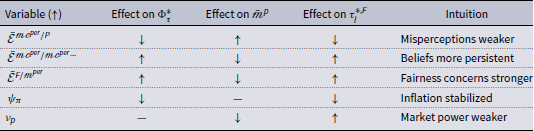
Table 1 presents the comparative statics of the optimal fiscal policy,
 $\tau _l^{*,F}$
. The sign of this policy is determined by the interplay between the strength of the behavioral biases, the degree of monopoly power, and the stance of monetary policy. As a result, the optimal intervention may manifest as either a labor subsidy or a tax. This outcome reflects the planner’s effort to balance efficiency objectives with the fairness-sensitive preferences embedded in household utility.
Comparative statics of the optimal fiscal policy
 $\tau _l^{*,F}$

Note: — indicates no direct effect. All signs report the effect of an increase in the corresponding variable on the steady-state values of
 $\Phi _\tau ^*$
,
 $\bar {\unicode{x1D4C2}}^{{p}}$
, and
 $\tau _l^{*,{F}}$
.
 $\bar {\mathcal{E}}^{\unicode{x1D4C2}\unicode{x1D4B8}^{per}/{P}}$
denotes the elasticity of perceived marginal costs with respect to prices.
 $\bar {\mathcal{E}}^{\unicode{x1D4C2}\unicode{x1D4B8}^{per}/\unicode{x1D4C2}\unicode{x1D4B8}^{per}-}$
captures the elasticity of current perceived marginal costs with respect to its lagged value.
 $\bar {\mathcal{E}}^{{F}/\unicode{x1D4C2}^{per}}$
refers to the elasticity of fairness concerns with respect to the perceived price markup. All elasticities are evaluated at their steady-state values. Further details are provided in Appendix A.2.4.
When
 $\bar {\mathcal{E}}^{\unicode{x1D4C2}\unicode{x1D4B8}^{per}/\unicode{x1D4C2}\unicode{x1D4B8}^{per}-}$
increases, the household’s perceived marginal cost becomes more persistent over time. This implies that the household’s beliefs regarding firm pricing behavior become increasingly anchored in past perceptions, thereby diminishing the rate at which the household updates its beliefs in response to current price signals. Consequently, fairness concerns intensify over time. This dynamic leads to a stronger accumulation of fairness-related distortions, thereby amplifying the effective fairness-weight,
 $\Phi _\tau ^*$
. Given the household’s response, the firm adjusts by decreasing its price markup to mitigate the impact of fairness-based perceptions on demand. As a result, the optimal labor subsidy is reduced. In extreme scenarios, the planner may determine that implementing a labor tax is the optimal policy choice in order to mitigate the household’s exposure to its fairness concerns.
Similarly, an increase in the elasticity
 $\bar {\mathcal{E}}^{F/\unicode{x1D4C2}^{per}}$
amplifies the sensitivity of the household to deviations in the perceived price markup. Under these conditions, changes in the household’s beliefs about firm behavior affect the fairness component of household utility more strongly. In response to this heightened sensitivity, the planner places greater emphasis on the fairness channel when evaluating welfare. As the effective fairness weight rises, the scope for optimal policy intervention narrows, leading to a reduction in the fiscal correction. In extreme cases, where behavioral distortions dominate, the planner may find it optimal to implement a labor tax.
An increase in
 $\nu _p$
, the elasticity of substitution across differentiated goods, reduces firm market power by flattening the demand curve. This results in a lower perceived markup,
 $\unicode{x1D4C2}^{per} = \frac {\nu _p}{\nu _p - 1}$
, as well as a lower fairness-adjusted markup,
 $\bar {\unicode{x1D4C2}}^p$
. Since both efficiency and behavioral distortions are tied to the size of this markup, a higher
 $\nu _p$
diminishes the need for fiscal correction. However,
 $\nu _p$
does not directly influence the fairness-weight, implying that the planner’s response to perceived fairness dynamics remains unchanged. Consequently, the labor subsidy decreases primarily due to weaker markup distortions. When fairness effects are moderate, the optimal policy continues to involve a subsidy, albeit a smaller one.
In contrast, an increase in
 $\bar {\mathcal{E}}^{\unicode{x1D4C2}\unicode{x1D4B8}^{per}/P}$
strengthens the relationship between households’ perceived marginal cost and observable price changes. This closer alignment reduces the potential for misperception, bringing perceived markups more in line with actual firm behavior. As a result, the fairness-weight decreases, reflecting a reduction in the utility penalty associated with misperceived pricing. This decline in behavioral distortions provides the planner with greater flexibility to address monopolistic inefficiencies, leading to a shift toward a more aggressive labor subsidy. In this case, the fairness model converges toward the standard NK benchmark, where behavioral distortions are negligible and the optimal policy almost fully offsets market power distortions.
Finally, an increase in the inflation coefficient
 $\psi _{\pi }$
intensifies the central bank’s responsiveness to deviations in inflation. A stronger monetary policy reaction stabilizes inflation expectations and anchors firms’ pricing decisions more effectively. This reduces the forward-looking component of perceived pricing distortions and curtails the dynamic accumulation of fairness concerns over time. Consequently, the fairness-weight declines, easing the planner’s welfare constraint. This relaxation enables the fiscal authority to implement a larger labor subsidy without generating excessive fairness-related disutility. This outcome highlights the complementary interaction between monetary policy and fairness-based distortions, as a more aggressive monetary stance broadens the scope for optimal fiscal correction within the NK framework.
In summary, the sign and magnitude of the optimal fiscal policy,
 $\tau _l^{*,F}$
, are shaped by the planner’s trade-off between addressing monopolistic distortions and respecting fairness preferences. When behavioral biases are significant, either due to the persistence of household beliefs or heightened sensitivity to markup deviations, the optimal policy may involve a labor tax. However, such a policy represents a second-best solution that fails to fully restore efficient allocations. By contrast, when behavioral distortions are sufficiently subdued, the planner can implement a strong labor subsidy, improving both allocations and welfare in accordance with the standard NK benchmark.
Importantly, if the optimal policy takes the form of a labor tax rather than a subsidy, a welfare loss is unavoidable. This stems from the planner’s inability to simultaneously offset monopolistic distortions and accommodate fairness preferences. A formal proof of this result is provided in Appendix A.2.4. Within this framework, welfare at the zero-inflation steady state is characterized by the utility function evaluated at the equilibrium level of labor, as follows
 \begin{equation*} \bar {\mathcal{W}} = \frac {\ln (\bar {L}) - \frac {\bar {L}^{1+\eta }}{1+\eta }}{1 - \beta } \end{equation*}
In the absence of any fiscal intervention, the steady-state level of labor is determined by
 \begin{equation*} \bar {L} = \left ( \frac {1}{\bar {\unicode{x1D4C2}}^{p} \unicode{x1D4C2}^{w,NK}} \right )^{\frac {1}{1+\eta }} \lt 1 \end{equation*}
If the planner instead implements its optimal fiscal policy, the resulting allocation is
 \begin{equation} \bar {L} = \left ( 1 - \Phi _\tau ^* \right )^{\frac {1}{1+\eta }} \lt 1 \end{equation}
A welfare loss relative to the no-policy case arises if and only if
 \begin{equation*} 1 - \Phi _\tau ^* \lt \frac {1}{\bar {\unicode{x1D4C2}}^{p} \unicode{x1D4C2}^{w,NK}} \end{equation*}
which occurs only if the policy is a tax. As shown in Table 1, this condition is likely to hold under (i) high fairness sensitivity, (ii) persistent belief distortions, and (iii) insufficiently stringent inflation stabilization by the central bank. Section 4 provides a numerical exploration of these cases.
Given the strong interaction between inflation dynamics and fairness-based distortions, an alternative policy approach involves directly regulating firms’ price-setting behavior through a price-cap-type mechanism. Under this formulation, the fiscal instrument is deactivated (
 $\tau _{l,t} = 0, \, \forall t$
), and the planner instead determines the optimal path of the price markup,
 $\unicode{x1D4C2}_t^{p,*}$
, directly. This approach shifts the focus from indirect fiscal interventions to direct control over firms’ pricing decisions, aiming to address both monopolistic distortions and perceived fairness dynamics at their source.
Let
 $\unicode{x1D4C2}^{gap} = \bar {\unicode{x1D4C2}}^p - \bar {\unicode{x1D4C2}}^{p,*}$
denote the gap between the competitive-equilibrium markup and the planner’s optimal markup. If
 $\unicode{x1D4C2}^{gap} \gt 0$
, the optimal markup policy implies a cap on firms’ pricing power. The next proposition establishes the closed-form expression for the optimal markup cap in steady-state.
Proposition 2. In a fairness model with monopolistic competition, Rotemberg price adjustment costs, and inflation-targeting monetary policy, the optimal price markup at the zero-inflation steady-state is given by
 \begin{equation} \bar {\unicode{x1D4C2}}^{p,*} = \frac {1}{1 - \Phi _\tau ^*} \end{equation}
where
 $\Phi _\tau ^* = - \bar {\mathcal{E}}^{F/\unicode{x1D4C2}^{per}} \cdot \frac {\big(1 - \bar {\mathcal{E}}^{\unicode{x1D4C2}\unicode{x1D4B8}^{per}/P}\big)(1 - \beta )}{(1 - \beta \bar {\mathcal{E}}^{\unicode{x1D4C2}\unicode{x1D4B8}^{per}/\unicode{x1D4C2}\unicode{x1D4B8}^{per,-}})(1 - \beta \psi _\pi )}$
.
Proof. Proof in Appendix A.2.5.
This expression mirrors the allocation obtained under an optimal labor subsidy. Specifically, the implied labor allocation is
 \begin{equation*} \bar {L} = \left ( \frac {1}{\bar {\unicode{x1D4C2}}^{p,*}} \right )^{\frac {1}{1+\eta }} = \left ( 1 - \Phi _\tau ^* \right )^{\frac {1}{1+\eta }} \lt 1 \end{equation*}
which is identical to the allocation achieved under the optimal labor subsidy, as shown in Equation (17). The equivalence of allocations emerges because, within this framework, the fiscal and regulatory approaches are functionally identical in addressing the underlying distortions. This leads to the following corollary.
Corollary 3.
In the fairness-augmented model, implementing an optimal price markup cap
 $\bar {\unicode{x1D4C2}}^p \gt \bar {\unicode{x1D4C2}}^{p,*}$
is equivalent to introducing an optimal labor subsidy
 $\tau _l^{*,F} \lt 0$
.
Proof. Proof in Appendix A.2.6.
This result underscores a conditional equivalence between regulatory and fiscal instruments in mitigating the monopoly and behavioral distortions within the model’s structure. Specifically, both a labor subsidy and a markup cap can be calibrated to achieve identical allocations, provided the planner fully internalizes the behavioral distortions associated with perceived fairness dynamics. While this theoretical equivalence is robust within the model, its practical implementation may vary. In real-world settings, the choice between fiscal and regulatory instruments is likely to be influenced by factors such as institutional feasibility, enforcement capacity, and overarching policy objectives.
The next section provides a quantitative illustration of the optimal fiscal policy, whether a labor subsidy or a tax, using parameter values calibrated to the EA economy. The fairness and inference functions are specified in accordance with the properties defined in Section 2. Under this specification, all theoretical results, including Propositions A.2.2 and A.2.5, and their corresponding corollaries, remain valid.
4. A fairness model for the euro area
4.1 Model summary
This section develops a generalized NK model of the EA economy that incorporates perceived fairness dynamics into a fully structural framework. It has two objectives. First, to demonstrate that the key equilibrium conditions from the stylized model arise as reduced-form representations of a full structural system (more details in Appendix B). Second to calibrate the model to EA data to assess the quantitative implications of fairness-based distortions for optimal fiscal policy.
The economy is populated by a continuum of households indexed by
 $ k \in [0,1]$
and a continuum of firms indexed by
 $ j \in [0,1]$
. Households supply differentiated labor services to a labor agency, which aggregates these into a composite input demanded by firms. Firms, in turn, produce differentiated final goods that are consumed by households. As a result, both labor and goods markets are monopolistically competitive, generating price and wage markups.
The structural model presented in that section preserves the behavioral assumptions utilized in the illustrative model. Aligned with the earlier framework, households develop beliefs about firms’ pricing behavior based on observed prices and an imperfect inference process, which, in turn, influence their consumption and labor decisions, as described in Eyster et al. (Reference Eyster, Madarász and Michaillat2021). Additionally, the current model introduces two significant extensions: first, it incorporates nominal price rigidities à la Rotemberg, (Reference Rotemberg1982), and second, it includes a Ramsey planner who is responsible for formulating the optimal fiscal policy to address fairness-induced misperceptions of price markups.
Monetary policy is conducted via an inflation-targeting rule, while fiscal policy is balanced through lump-sum transfers. The equilibrium is defined over twelve variables: the true and perceived markups
 $ \unicode{x1D4C2}_{t}^p$
,
 $ \unicode{x1D4C2}_t^{p,per}$
, inflation
 $ \pi _t$
, the nominal interest rate
 $ i_t$
, output
 $ Y_t$
, labor
 $ L_t$
, consumption
 $ C_t$
, productivity
 $ A_t$
, the real wage
 $ w_t$
, the fairness judgments
 $ F_t$
, the price elasticity of demand
 $ \mathcal{E}_t^{Y/P}$
, and the inflation-cost
 $ \Upsilon _t$
. The optimal labor subsidy
 $ \tau _{l,t}^*$
is chosen by the planner to maximize household welfare, subject to behavioral and structural constraints.
For full derivations and model equations, see Appendix B.
4.2 Optimal policy and welfare
At equilibrium, households form expectations about firms’ marginal costs using a Cobb-Douglas inference rule
 \begin{equation} \unicode{x1D4C2}\unicode{x1D4B8}_t^{per} = \left ( \unicode{x1D4C2}\unicode{x1D4B8}_{t-1}^{per} \right )^{\gamma _p} \left ( \frac {P_t}{\bar {\unicode{x1D4C2}}^{p,per}} \right )^{1 - \gamma _p} \end{equation}
where
 $ \gamma _p \in (0,1)$
governs the inertia of belief updating and
 $ \bar {\unicode{x1D4C2}}^{p,per}$
is the reference price markup used by households. This formulation implies that beliefs about marginal costs combine persistent past expectations with current price information
 $ P_t$
, adjusted by a fairness-based normalization.Footnote
12
By definition, the perceived price markup is given by
 $ \unicode{x1D4C2}_t^{p,per} = \frac {P_t}{\unicode{x1D4C2}\unicode{x1D4B8}_t^{per}}$
. Combining this expression with the Cobb-Douglas form of
 $ \unicode{x1D4C2}\unicode{x1D4B8}_t^{per}$
yields
 \begin{equation} \unicode{x1D4C2}_t^{p,per} = \left ( \unicode{x1D4C2}_{t-1}^{p,per} \cdot \pi _t \right )^{\gamma _p} \left ( \bar {\unicode{x1D4C2}}^{p,per} \right )^{1 - \gamma _p} \end{equation}
where
 $ \pi _t = P_t / P_{t-1}$
denotes the gross inflation rate. This shows that the perceived markup itself inherits a Cobb-Douglas structure as a function of inflation and lagged perceived markup.
Fairness concerns are modeled separately via a linear penalty in utility. Households experience disutility when firms are perceived to price unfairly. This occurs when the perceived markup deviates from a fairness benchmark, which is defined as its steady-state value in this context
 \begin{equation} F_t = 1 - \theta _p \left ( \unicode{x1D4C2}_t^{p,per} - \bar {\unicode{x1D4C2}}^{p,per} \right ) \end{equation}
where the steady-state perceived markup is given by
 $ \bar {\unicode{x1D4C2}}^{p,per} = \frac {\nu _p}{\nu _p - 1}$
, a level consistent with the standard NK model. This reflects the assumption that, under a zero-inflation steady-state, fairness concerns are fully resolved. The strength of fairness preferences is governed by the parameter
 $ \theta _p \gt 0$
, which measures the sensitivity to perceived unfairness. This linear specification ensures tractability while capturing the additive disutility associated with deviations in perceived fairness.
The fairness and inference mechanisms imply that fluctuations in inflation directly give rise to behavioral biases through their effect on perceived markups. Since the planner cannot directly influence the process of belief formation, optimal fiscal policy must instead stabilize fairness through indirect means, primarily by reducing households’ exposure to inflation. The planner does so by adjusting the optimal policy rate
 $ \tau _l$
in response to behavioral biases, which are summarized by the composite fairness-weight
 \begin{equation} \Phi _\tau ^{EA} = - \frac { \theta _p \gamma _p \bar {\unicode{x1D4C2}}^{p,per} (1 - \beta ) }{ (1 - \beta \gamma _p)(1 - \beta \psi _\pi )} \in (0,1) \end{equation}
This fairness-weight enters the optimal policy rule
 \begin{equation} \tau _l^{*,EA} = 1 - \big(1 - \Phi _\tau ^{EA}\big) \, \bar {\unicode{x1D4C2}}^p \, \unicode{x1D4C2}^{w,NK} \end{equation}
where
 $ \bar {\unicode{x1D4C2}}^p$
is the steady-state competitive markup and
 $ \unicode{x1D4C2}^{w,NK}$
the NK wage markup. A higher
 $\Phi _\tau ^{EA}$
reduces the magnitude of the optimal labor subsidy (or raises the labor tax), reflecting the planner’s trade-off between market efficiency and fairness disutility.
An increase in
 $ \gamma _p$
indicates that households’ beliefs about firms’ behavior become more persistent and more sensitive to inflation. This amplifies behavioral distortions through stronger perceived markup fluctuations, which raises the fairness-weight
 $ \Phi _\tau ^{EA}$
and leads the planner to reduce the labor subsidy, or possibly impose a labor tax, to contain inflation. In the limiting case where
 $ \gamma _p \to 0$
, belief updating becomes fully myopic and fairness misperceptions disappear. In this case,
 $ \Phi _\tau ^{EA} \to 0$
, and the optimal policy converges to the standard NK benchmark, fully offsetting all distortions.
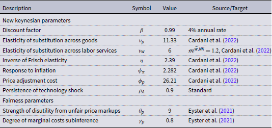
The model was calibrated to represent a quarterly time frequency. Parameter values are reported in Table 2. The discount factor
 $\beta$
has a standard value of 0.99 to achieve a 4% annual rate. The elasticity of substitution across goods 11.335
 $(\nu _p)$
, the wage markup 1.20
 $\left (\unicode{x1D4C2}^{w,NK} = \frac {\nu _w}{\nu _w - 1}\right )$
, the inverse Frisch elasticity 2.39
 $(\eta )$
, the price adjustment cost 26.21
 $(\phi _p)$
, and the response of nominal interest rate to inflation 2.282
 $(\psi _\pi )$
are taken from Cardani et al. (Reference Cardani, Croitorov, Giovannini, Pfeiffer, Ratto and Vogel2022).
Parameter values

The parameters related to the price markup fairness, namely the degrees of marginal costs subinference
 $ \gamma _p$
and the strength of disutility from unfair price markups
 $ \theta _p$
, were calibrated jointly to generate an instantaneous and two-year cost pass-through to prices of 0.4 and 0.7, respectively, in line with the microeconomic evidence reported by Eyster et al. (Reference Eyster, Madarász and Michaillat2021). The triplet
 $ \{\theta _p, \gamma _p, \nu _p\}$
yields a steady-state price markup
 $ \bar {\unicode{x1D4C2}}^p$
of 1.07.
In this model calibration, with
 $ \gamma _p = 0.8$
,
 $ \theta _p = 9$
, and
 $ \psi _\pi = 2.282$
, the fairness weight is quantitatively significant. The resulting optimal fiscal policy entails a labor tax rate of approximately 10 percent, corresponding to an optimal price markup of 1.19, 12 percentage points higher than the steady-state level. This represents a constrained second-best outcome, in which the planner imposes an elevated price markup as a trade-off to curb household spending and alleviate fairness concerns. Under the calibration, the planner chooses a tax rather than a subsidy precisely to dampen spending that would otherwise exacerbate perceived unfairness, thereby improving welfare in the presence of belief-formation frictions.
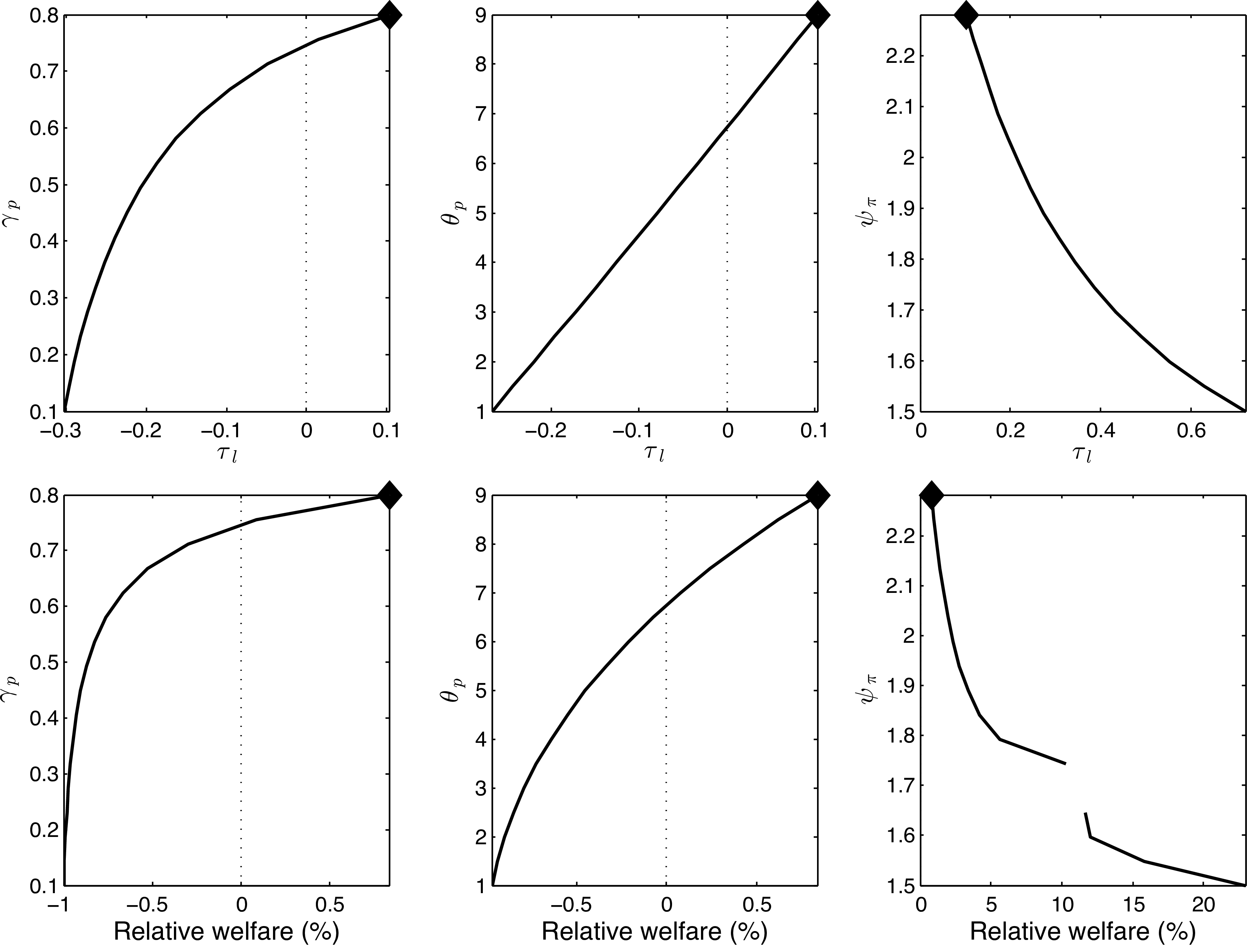
Furthermore, the top panels of Figure 1 show that a reduction in either
 $ \gamma _p$
or
 $ \theta _p$
leads to a policy shift toward a labor subsidy, effectively operating as a price markup cap. In addition, the third panel in the top row demonstrates that a more accommodative monetary stance, reflected by a lower inflation response coefficient
 $ \psi _\pi$
, raises the steady-state labor tax rate substantially, reaching up to 70% for a conventional Taylor-rule value of
 $ \psi _\pi = 1.5$
. This underscores the importance of coordinated monetary and fiscal policy: without such coordination, significant welfare losses may arise due to excessive taxation required to contain behavioral distortions.
Optimal labor subsidy/tax and relative welfare.
Note: The optimal policy and the associated relative welfare in the benchmark calibration are represented by diamonds (
 $\gamma _p = 0.8$
,
 $\theta _p = 9$
, and
 $\psi _\pi = 2.282$
). Steps of 0.5 were used for
 $\theta _p$
, representing 17 values
 $\in [1,9]$
. In turn, 15 values were evenly sliced in
 $[0.1, 0.8]$
and
 $[1.5, 2.282]$
for
 $\gamma _p$
and
 $\psi _\pi$
, respectively. The relative welfare when
 $\psi _\pi \approx 1.7$
is dropped because it leads to an outlier. Welfare is defined as:
 $\mathbb{E}_t(\mathcal{W}_t) = \mathbb{E}_t(\ln (\mathcal{C}_t) - L_t^{1+\eta }/(1+\eta ) + \beta \mathbb{E}_t \mathcal{W}_{t+1})$
and the standard deviation of the technology shock is set to 1%. Relative welfare is calculated as
 $\exp ((1-\beta ) (\mathbb{E}_t(\mathcal{W}_t)^{no pol.} - \mathbb{E}_t(\mathcal{W}_t)^{EA})) -1$
where
 $\mathbb{E}_t(\mathcal{W}_t)^{no pol.}$
is the welfare expectation in the EA model without labor subsidy/tax. Relative welfare represents the fairness-consumption percentage that households would be willing to forgo to remain in the fairness economy but free of labor subsidy/tax. In other words, if the relative welfare is positive (negative), the optimal policy results in a welfare loss (gain) relative to an economy with no policy.

Regarding welfare implications, the lower panels of Figure 1 display relative welfare. Welfare is defined as
 \begin{equation*} \mathbb{E}_t(\mathcal{W}_t) = \mathbb{E}_t\!\left (\ln (\mathcal{C}_t) - \tfrac {L_t^{1+\eta }}{1+\eta } + \beta \mathbb{E}_t \mathcal{W}_{t+1}\right ) \end{equation*}
where the standard deviation of the technology shock is set to 1%. Relative welfare is calculated as
 \begin{equation*} \exp \!\left((1-\beta )\left(\mathbb{E}_t(\mathcal{W}_t)^{no\, pol.} - \mathbb{E}_t(\mathcal{W}_t)^{EA}\right)\right) -1 \end{equation*}
where
 $\mathbb{E}_t(\mathcal{W}_t)^{no\, pol.}$
denotes expected welfare in the EA model without a labor subsidy or tax. Relative welfare therefore measures the percentage of fairness-adjusted consumption that households would be willing to forgo to remain in the fairness economy but free of labor subsidy or tax.
Under the benchmark calibration (marked by diamonds), the welfare loss, indicated by positive values of relative welfare is modest, amounting to approximately 0.75% of steady-state consumption. This reflects households’ willingness to sacrifice consumption in exchange for avoiding the moderate optimal tax of around 10%. When fairness considerations weaken and the policy shifts toward a labor subsidy, as shown in the first two panels, welfare gains emerge but remain limited, peaking at roughly 1% of consumption.
Values for
 $\tau _l^{EA}$
.
Note: Steps of 0.1 were used for
 $\theta _p$
, representing 17 values
 $\in [1,9]$
. In turn, 80 values were evenly sliced in the interval
 $[0.1, 0.8]$
for
 $\gamma _p$
. The color bar on the right-hand side indicates whether the optimal policy is a labor subsidy or a tax.

In contrast, welfare losses increase substantially under looser inflation targeting when households exhibit both strong fairness concerns and persistent myopic behavior, characterized by
 $\gamma _p = 0.8$
and
 $\theta _p = 9$
. For example, under a standard inflation-targeting regime with
 $\psi _\pi = 1.5$
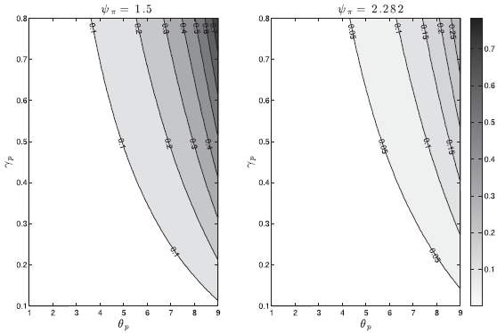
, households would be willing to forgo roughly 25% of their consumption to avoid the labor tax. As shown in the left panel of Figure 2, the corresponding tax rate can approach 70%, leading to sizable steady-state distortions in labor. This underscores the importance of a strong inflation-targeting regime for preserving the effectiveness of optimal fiscal policy in the presence of fairness concerns and belief inertia. The calibration results in the same figure also indicate that, across a broad range of values for
 $\theta _p$
and
 $\gamma _p$
, the optimal policy remains a labor subsidy provided that monetary policy responds aggressively to inflation. While fairness parameters do influence the planner’s trade-off, the strength of the monetary response emerges as a more decisive factor in determining the sign of the optimal fiscal policy, at least when behavioral distortions remain in the mild to moderate range.Footnote
13
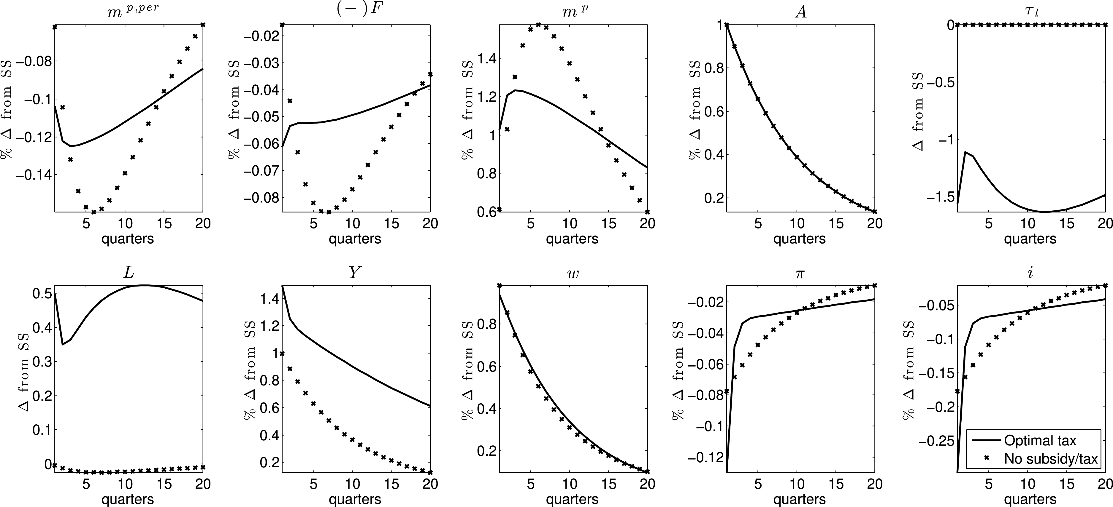
Finally, Figure 3 illustrates the model dynamics under the benchmark calibration following an unanticipated, transitory 1% increase in the technology level.Footnote 14 The figure compares the responses of key variables in an economy without fiscal intervention to those under the optimal fiscal policy, which features a steady-state labor tax of approximately 10%.
The positive technology shock generates distinct dynamic responses depending on the implementation of an optimal fairness-aware tax policy. In both scenarios, the shock reduces marginal costs and prices. However, perceived price markups decline more sharply in the absence of taxation. This steeper decline reflects a greater reduction in households’ fairness concerns when taxation is not implemented. Under the optimal tax policy, however, this improvement is moderated. Although this policy response may appear counterintuitive, since price decreases following a positive technology shock reduce perceived price markups, the policy is specifically designed to minimize fairness concerns across all types of technology shocks, both positive and negative, in order to mitigate all forms of distortions. In fact, the response of true price markups to a positive technology shock is more constrained when the optimal policy is in place.
Positive technology shock in the EA model.
Note: ”Optimal tax” refers to the variable responses to the technology shock under the Ramsey allocations (details in Appendix A.3). It should be noted that at steady-state, under the benchmark calibration, the optimal policy is a tax of about 10%. ”No subsidy/tax” refers to the variable responses to the shock in the EA model under the same calibration but without a labor subsidy/tax. Both models are calibrated similarly, with parameter values given in Table 2. The negative sign
 $(-) F$
reflects a reversal of the original sign, aiding interpretation in terms of fairness concerns.

Labor supply responds more robustly under the optimal tax policy due to the gradual reduction in labor tax over time. Lower tax raises net labor income, enhancing incentives for labor supply and driving a greater expansion of output compared to the scenario without fiscal intervention. Inflation declines in both cases, but the reduction is less pronounced with the optimal tax policy. This occurs because the policy reduces labor tax to stimulate demand and counteract downward price pressures arising from the technological shock.
A defining feature of the optimal fiscal policy is its time-varying nature, which adapts to shifting behavioral responses throughout the transition process. As the shock unfolds, the labor tax is incrementally reduced, providing a stimulus that addresses fairness concerns and perceived markup volatility. This contrasts with the standard NK framework, where the fiscal instrument is a constant labor subsidy aimed at addressing monopoly distortions, which are also constant across states.
5. Conclusion
This study builds upon the analytical framework of Eyster et al. (Reference Eyster, Madarász and Michaillat2021) by employing a NK model that integrates fairness considerations to examine optimal policy design in economies characterized by behaviorally salient fairness concerns. The model is characterized by monopolistic competitions, Rotemberg price adjustment costs, and inflation-targeting monetary policy, enabling a detailed examination of how fairness-driven behavioral biases influence macroeconomic outcomes and policy trade-offs. By embedding households’ preferences over perceived price markups into the NK framework, the analysis reveals that fairness concerns meaningfully alter the design of optimal fiscal and regulatory policies.
Specifically, the inclusion of fairness considerations leads to a departure from the standard NK benchmark, which typically prescribes a constant and permanent labor subsidy. Perceived fairness dynamics weaken the planner’s willingness to fully offset monopoly-induced distortions, as households’ misperceptions of price markups introduce additional welfare trade-offs. In cases where perceived fairness dynamics are particularly strong, the optimal policy may involve a labor tax instead of a subsidy, reflecting the planner’s prioritization of mitigating welfare losses arising from fairness-related behavioral distortions over achieving allocative efficiency. Furthermore, the optimal fiscal policy is not constant but instead adjusts in response to the evolution of behavioral distortions across states.
Comparative static analysis underscores the critical role of behavioral elasticities and the stance of monetary policy in shaping the planner’s policy choices. When households exhibit greater persistence in their fairness misperceptions or heightened sensitivity to fairness concerns, the effective distortion becomes more pronounced. This weakens the case for labor income subsidies and increases the likelihood that the planner will resort to taxation. Conversely, a stronger inflation-targeting monetary regime mitigates fairness concerns by anchoring expectations and stabilizing perceived price markups. This, in turn, reduces the behavioral distortions associated with fairness concerns and broadens the scope for traditional subsidy-based interventions. These findings highlight the importance of coordination between monetary and fiscal policy in economies where fairness considerations are behaviorally salient.
The analysis also explores an alternative regulatory policy aimed at addressing fairness-related distortions: directly capping firms’ price markups. Such a regulatory intervention can replicate the real allocations achieved through fairness-adjusted labor subsidy, thereby offering a theoretically equivalent mechanism for reducing welfare losses. While not a prescriptive recommendation, this approach highlights the conceptual substitutability between fiscal and market-based interventions, especially in contexts where fairness-driven distortions weaken the effectiveness of traditional policy tools.
The findings of this study suggest that fairness perceptions, while often considered psychological factors, may play a meaningful role in shaping macroeconomic policy outcomes. Overlooking these considerations could lead to unintended biases in policy design and potential welfare losses. Policymakers may benefit from incorporating fairness concerns into fiscal and monetary interventions aimed at addressing market distortions and promoting economic stability. Future research could explore the empirical measurement of fairness preferences, their persistence, and their broader economic implications. Approaches such as experimental studies, surveys, and the analysis of detailed price and consumption data may provide valuable insights into how fairness considerations influence policy effectiveness.
Acknowledgments
I would like to thank Aurélien Eyquem and Pascal Michaillat for their suggestions and valuable comments. I am also grateful to two anonymous referees, the associate editor, and the editor for their insightful feedback and constructive remarks.
Appendix A.
A.1 Illustrative fairness model: derivations
Notation clarification
When I write derivatives like
 $\frac {d f(x)}{d x}$
, I always refer to the derivative of the full, substituted expression for
 $f(x)$
, accounting for all dependencies of
 $f$
on
 $x$
. This applies whether
 $f(x)$
is written explicitly or as a shorthand for a composite mapping. I apply the same convention to partial derivatives such as
 $\frac {\partial f(x, y)}{\partial x}$
.
The household’s expected lifetime utility is
 \begin{equation*} \mathbb{E}_0 \sum _{t=0}^\infty \beta ^t \left ( u(\mathcal{C}_t) - v(L_t) \right ) \end{equation*}
The budget constraint is
 \begin{equation*} (1-\tau _{l,t}) \frac {W_t}{\mathcal{P}_t} L_t + i_{t-1} \frac {B_{t-1}}{\mathcal{P}_t} + \Pi _t + T_{t} = \frac {B_t}{\mathcal{P}_t} + \mathcal{C}_t \end{equation*}
The household chooses
 $\mathcal{C}_t = C_t F_t$
,
 $L_t$
,
 $W_t$
, and
 $B_t$
under the budget constraint and labor demand,
 $L_t = W_t^{-\nu _w}$
. FOCs,
 \begin{eqnarray*} \mathcal{C}_t: \quad && \lambda _t^c = u'(\mathcal{C}_t) \\ B_t: \quad && \lambda _t^c = i_t \beta \mathbb{E}_t \left ( \lambda _{t+1}^c \frac {\mathcal{P}_t}{\mathcal{P}_{t+1}} \right ) \\ L_t: \quad && \mu _t^c = -v'(L_t) + \lambda _t^c (1-\tau _{l,t}) \frac {W_t}{\mathcal{P}_t} \\ W_t: \quad && \nu _w \mu _t^c \frac {L_t}{W_t} = \lambda _t^c (1-\tau _{l,t}) \frac {L_t}{\mathcal{P}_t} \end{eqnarray*}
then,
 \begin{eqnarray*} B_t: \quad && 1 = i_t \beta \mathbb{E}_t \left ( \frac {u'(\mathcal{C}_{t+1})}{u'(\mathcal{C}_t)} \frac {\mathcal{P}_t}{\mathcal{P}_{t+1}} \right ) \\[5pt] L_t: \quad && \frac {1}{v'(L_t)} \mu _t^c = -1 + \frac {u'(\mathcal{C}_t)}{v'(L_t)} (1-\tau _{l,t}) \frac {W_t}{\mathcal{P}_t} \\ W_t: \quad && \frac {\nu _w}{v'(L_t)} \mu _t^c = \frac {u'(\mathcal{C}_t)}{v'(L_t)} (1-\tau _{l,t}) \frac {W_t}{\mathcal{P}_t} \end{eqnarray*}
let
 $\unicode{x1D4C2}^{w,NK} = \frac {u'(\mathcal{C}_t)}{v'(L_t)} (1-\tau _{l,t}) w_t$
, where
 $w_t = \frac {W_t}{\mathcal{P}_t}$
,
 \begin{eqnarray*} L_t: \quad && \frac {1}{v'(L_t)} \mu _t^c = -1 + \unicode{x1D4C2}^{w,NK} \\[5pt] W_t: \quad && \nu _w \big(-1 + \unicode{x1D4C2}^{w,NK}\big) = \unicode{x1D4C2}^{w,NK} \end{eqnarray*}
consequently,
 $\unicode{x1D4C2}^{w,NK} = \frac {\nu _w}{\nu _w-1}$
.
The representative firm produces output under a simple technology
 $Y_t = A_t L_t$
, where
 $A_t$
is a technology shock. The present value of its expected profits (
 $\Pi _t$
) is
 \begin{eqnarray*} &&\mathbb{E}_0 \sum _{t=0}^\infty \Gamma ^t \left ( \frac {P_t}{\mathcal{P}_t} Y_t - \frac {W_t}{\mathcal{P}_t} L_t - \frac {\phi _p}{2} \left ( \frac {P_t}{P_{t-1}} - 1 \right )^2 \mathcal{C}_t \right ) \\[5pt] \triangleq &&\mathbb{E}_0 \sum _{t=0}^\infty \Gamma ^t \left (\left ( P_t - \unicode{x1D4C2}\unicode{x1D4B8}_t \right ) \frac {Y_t}{\mathcal{P}_t} - \frac {\phi _p}{2} \left ( \frac {P_t}{P_{t-1}} - 1 \right )^2 \mathcal{C}_t \right ) \end{eqnarray*}
where
 $\unicode{x1D4C2}\unicode{x1D4B8}_t = \frac {W_t}{A_t}$
. The firm maximizes its discounted profit by choosing
 $P_t$
,
 $Y_t$
, and
 $\unicode{x1D4C2}\unicode{x1D4B8}_t^{per}$
subject to the good demand,
 $Y_t = P_t^{-\nu _p} (\mathbb{F} (\unicode{x1D4C2}_t^{per}))^{\nu _p-1}$
, and the inference function,
 $\unicode{x1D4C2}\unicode{x1D4B8}_t^{per} = \mathbb{C} (\omega _p P_t, \unicode{x1D4C2}\unicode{x1D4B8}_{t-1}^{per})$
. Note that
 $\unicode{x1D4C2}\unicode{x1D4B8}_t^{per} = \mathbb{C} (\omega _p P_t, \unicode{x1D4C2}\unicode{x1D4B8}_{t-1}^{per})$
,
 $\mathbb{R}_+^2 \to \mathbb{R}_+$
, is a continuous function, twice differentiable, positive
 $\mathbb{C}(.,.) \gt 0$
, and satisfies
 $\mathbb{C}_i^{'} \gt 0$
,
 $\mathbb{C}_i^{''} \lt 0$
for
 $i \in \{P_t, \unicode{x1D4C2}\unicode{x1D4B8}_{t-1}^{per}\}$
and homogeneous of degree 1;
 $\omega _p$
is a positive wedge that determines the steady value of the perceived price markup. Finally, the perceived price markup is
 $\unicode{x1D4C2}_t^{per} = \frac {P_t}{\unicode{x1D4C2}\unicode{x1D4B8}_t^{per}}$
. FOCs,
 \begin{eqnarray*} Y_t: \quad && \lambda _t = \frac {P_t}{\mathcal{P}_{\unicode{x1D4C9}}} - \frac {\unicode{x1D4C2}\unicode{x1D4B8}_t}{\mathcal{P}_{\unicode{x1D4C9}}} = \frac {P_t}{\mathcal{P}_{\unicode{x1D4C9}}} \Delta \unicode{x1D4C2}_t^p \\[5pt] P_t: \quad && 0 = \frac {Y_t}{\mathcal{P}_{\unicode{x1D4C9}}} + \lambda _t \frac {\partial Y_t}{\partial P_t} + \mu _t \frac {\partial \unicode{x1D4C2}\unicode{x1D4B8}_t^{per}}{\partial P_t} - \phi _p \left (\frac {P_t}{P_{t-1}} - 1\right ) \frac {\mathcal{C}_{\unicode{x1D4C9}}}{P_{t-1}}\\[5pt] & &\qquad + \phi _p \mathbb{E}_t \left ( \Gamma _t \left (\frac {P_{t+1}}{P_t} - 1\right ) \frac {P_{t+1} \mathcal{C}_{{\unicode{x1D4C9}+1}}}{P_t^2}\right ) \\[5pt] \unicode{x1D4C2}\unicode{x1D4B8}_t^{per}: \quad && \mu _t = \mathbb{E}_t \left ( \Gamma _t \left ( \mu _{t+1} \frac {\partial \unicode{x1D4C2}\unicode{x1D4B8}_{t+1}^{per}}{\partial \unicode{x1D4C2}\unicode{x1D4B8}_{t}^{per}} + \lambda _{t+1} \frac {\partial Y_{t+1}}{\partial \unicode{x1D4C2}\unicode{x1D4B8}_{t}^{per}} \right ) \right ) \end{eqnarray*}
where,
 $\unicode{x1D4C2}_t^p = \frac {P_t}{mc_t}$
, and
 $\Delta \unicode{x1D4C2}_t^p = \frac {\unicode{x1D4C2}_t^p-1}{\unicode{x1D4C2}_t^p}$
. Multiply the second condition by
 $-\frac {\mathcal{P}_t}{Y_t}$
,
 \begin{eqnarray*} P_t: && 1 = - \lambda _t \frac {\partial Y_t}{\partial P_t} \frac {\mathcal{P}_t}{Y_t} - \mu _t \frac {\partial \unicode{x1D4C2}\unicode{x1D4B8}_t^{per}}{\partial P_t} \frac {\mathcal{P}_t}{Y_t} + \phi _p \left (\frac {P_t}{P_{t-1}} - 1\right ) \frac {\mathcal{P}_t}{P_{t-1}} \frac {\mathcal{C}_t}{Y_t}\\&& \qquad - \phi _p \mathbb{E}_t \left ( \Gamma _t \left (\frac {P_{t+1}}{P_t} - 1\right ) \frac {P_{t+1} \mathcal{P}_{\unicode{x1D4C9}}}{P_t^2} \frac {\mathcal{C}_{{\unicode{x1D4C9}+1}}}{Y_t} \right ) \\ \Longleftrightarrow && 1 = - \Delta \unicode{x1D4C2}_t^p \frac {\partial \ln (Y_t)}{\partial \ln (P_t)} - \mu _t \frac {\partial \unicode{x1D4C2}\unicode{x1D4B8}_t^{per}}{\partial P_t} \frac {\mathcal{P}_t}{Y_t} + \Upsilon _t \end{eqnarray*}
where
 $\Upsilon _t = \phi _p \big(\left ( \pi _t - 1\right ) \pi _t \frac {C_t}{Y_t} - \mathbb{E}_t \big( \Gamma _t \left ( \pi _{t+1} - 1\right ) \pi _{t+1} \frac {F_{t+1}}{F_t} \frac {C_{t+1}}{Y_t} \big) \big)$
. Then,
 \begin{eqnarray*} P_t: \quad \quad && 1 = - \Delta \unicode{x1D4C2}_t^p \frac {\partial \ln (Y_t)}{\partial \ln (P_t)} - \mu _t \frac {\partial \unicode{x1D4C2}\unicode{x1D4B8}_t^{per}}{\partial P_t} \frac {\mathcal{P}_t}{Y_t} + \Upsilon _t \\ \unicode{x1D4C2}\unicode{x1D4B8}_t^{per}: \quad \quad && \mu _t = \mathbb{E}_t \left ( \Gamma _t \left ( \mu _{t+1} \frac {\partial \unicode{x1D4C2}\unicode{x1D4B8}_{t+1}^{per}}{\partial \unicode{x1D4C2}\unicode{x1D4B8}_{t}^{per}} + \lambda _{t+1} \frac {\partial Y_{t+1}}{\partial \unicode{x1D4C2}\unicode{x1D4B8}_{t}^{per}} \right ) \right ) \end{eqnarray*}
define
 $\mathcal{E}_t^{Y/P} = -\frac {\partial \ln (Y_t)}{\partial \ln (P_t)} = \nu _p + (\nu _p-1) \Psi _t$
, where
 $\Psi _t = -\frac {d \ln (F_t)}{d \ln (\unicode{x1D4C2}_t^{per})} \left (1-\frac {\partial \ln \big(\unicode{x1D4C2}\unicode{x1D4B8}_t^{per}\big)}{\partial \ln (P_t)}\right )$
, then
 $\frac {\partial \ln (Y_t)}{\partial \ln \big(\unicode{x1D4C2}\unicode{x1D4B8}_{t-1}^{per}\big)} = (\nu _p-1) \Psi _t = \mathcal{E}_t^{Y/P} -\nu _p$
. By
 $\mathbb{C}$
’s degree of homogeneity,
 $\frac {\partial \ln (\unicode{x1D4C2}\unicode{x1D4B8}_t^{per})}{\partial \ln (P_t)} \lt 1$
 $\Rightarrow$
 $\left (1-\frac {\partial \ln (\unicode{x1D4C2}\unicode{x1D4B8}_t^{per})}{\partial \ln (P_t)}\right ) \gt 0$
. Then,
 \begin{eqnarray*} P_t: \quad \quad && \mu _t \frac {\partial \unicode{x1D4C2}\unicode{x1D4B8}_t^{per}}{\partial P_t} \frac {\mathcal{P}_t}{Y_t} = \Delta \unicode{x1D4C2}_t^p \mathcal{E}_t^{Y/P} - 1 + \Upsilon _t \\ \unicode{x1D4C2}\unicode{x1D4B8}_t^{per}: \quad \quad && \mu _t = \mathbb{E}_t \left ( \Gamma _t \left ( \mu _{t+1} \frac {\partial \unicode{x1D4C2}\unicode{x1D4B8}_{t+1}^{per}}{\partial \unicode{x1D4C2}\unicode{x1D4B8}_{t}^{per}} + \frac {P_{t+1}}{\mathcal{P}_{t+1}} \Delta \unicode{x1D4C2}_{t+1}^p \left(\mathcal{E}_{t+1}^{Y/P} -\nu _p\right) \frac {Y_{t+1}}{\unicode{x1D4C2}\unicode{x1D4B8}_{t}^{per}} \right ) \right ) \end{eqnarray*}
then,
 \begin{eqnarray*} \unicode{x1D4C2}\unicode{x1D4B8}_t^{per}: \quad \Delta \unicode{x1D4C2}_t^p \mathcal{E}_t^{Y/P} - 1 + \Upsilon _t &=& \mathbb{E}_t \Bigg ( \Gamma _t \Bigg ( \mu _{t+1} \frac {\partial \unicode{x1D4C2}\unicode{x1D4B8}_{t+1}^{per}}{\partial \unicode{x1D4C2}\unicode{x1D4B8}_{t}^{per}} \frac {\partial \unicode{x1D4C2}\unicode{x1D4B8}_{t}^{per}}{\partial P_{t}} \frac {\mathcal{P}_{t}}{Y_{t}} \\ &&+ \frac {P_{t+1}}{\mathcal{P}_{t+1}} \Delta \unicode{x1D4C2}_{t+1}^p \left(\mathcal{E}_{t+1}^{Y/P} -\nu _p\right) \frac {Y_{t+1}}{\unicode{x1D4C2}\unicode{x1D4B8}_{t}^{per}} \frac {\partial \unicode{x1D4C2}\unicode{x1D4B8}_{t}^{per}}{\partial P_{t}} \frac {\mathcal{P}_{t}}{Y_{t}} \Bigg ) \Bigg ) \\ &=& \mathbb{E}_t \Bigg ( \Gamma _t \frac {Y_{t+1} P_{t+1} \mathcal{P}_t}{Y_t P_t \mathcal{P}_{t+1}} \Bigg ( \mathcal{E}_t^{\unicode{x1D4C2}\unicode{x1D4B8}^{per}/P} \mathcal{E}_{t+1}^{\unicode{x1D4C2}\unicode{x1D4B8}^{per}/\unicode{x1D4C2}\unicode{x1D4B8}^{per}-} \left ( \mathcal{E}_{t+1}^{\unicode{x1D4C2}\unicode{x1D4B8}^{per}/P} \right )^{-1} \\ && \left(\Delta \unicode{x1D4C2}_{t+1}^p \mathcal{E}_{t+1}^{Y/P} - 1 + \Upsilon _{t+1}\right) + \Delta \unicode{x1D4C2}_{t+1}^p \left(\mathcal{E}_{t+1}^{Y/P} -\nu _p\right) \mathcal{E}_t^{\unicode{x1D4C2}\unicode{x1D4B8}^{per}/P} \Bigg ) \Bigg ) \\ &=& \beta \mathbb{E}_t \Bigg ( \mathcal{E}_t^{\unicode{x1D4C2}\unicode{x1D4B8}^{per}/P} \mathcal{E}_{t+1}^{\unicode{x1D4C2}\unicode{x1D4B8}^{per}/\unicode{x1D4C2}\unicode{x1D4B8}^{per}-} \left ( \mathcal{E}_{t+1}^{\unicode{x1D4C2}\unicode{x1D4B8}^{per}/P} \right )^{-1} \\ && \times \left(\Delta \unicode{x1D4C2}_{t+1}^p \mathcal{E}_{t+1}^{Y/P} - 1 + \Upsilon _{t+1}\right)\\ && + \Delta \unicode{x1D4C2}_{t+1}^p \left(\mathcal{E}_{t+1}^{Y/P} -\nu _p\right) \mathcal{E}_t^{\unicode{x1D4C2}\unicode{x1D4B8}^{per}/P} \Bigg ) \end{eqnarray*}
where
 $\mathcal{E}_t^{\unicode{x1D4C2}\unicode{x1D4B8}^{per}/P} = \frac {\partial \ln (\unicode{x1D4C2}\unicode{x1D4B8}_{t}^{per})}{\partial \ln (P_{t})}$
, and
 $\mathcal{E}_t^{\unicode{x1D4C2}\unicode{x1D4B8}^{per}/\unicode{x1D4C2}\unicode{x1D4B8}^{per}-} = \frac {\partial \ln (\unicode{x1D4C2}\unicode{x1D4B8}_{t}^{per})}{\partial \ln \big(\unicode{x1D4C2}\unicode{x1D4B8}_{t-1}^{per}\big)}$
. The last equality holds assuming
 $u(C_t F_t) = \ln (C_t F_t)$
and
 $C_t = Y_t$
, therefore
 $\Gamma _t = \beta \frac {u'(\mathcal{C}_{t+1})}{u'(\mathcal{C}_t)} = \beta \frac {C_t F_t}{C_{t+1} F_{t+1}}$
. The good market clearing is
 $C_t \left (1+\frac {\phi _p}{2} (\pi _t-1)^2\right ) = Y_t$
.
For instance, one can assume that the inference function of the perceived marginal costs is a Cobb-Douglas with an elasticity
 $\gamma _p \in (0,1)$
as in Eyster et al. (Reference Eyster, Madarász and Michaillat2021):
 $\unicode{x1D4C2}\unicode{x1D4B8}_t^{per} = \left (\frac {\nu _p-1}{\nu _p} P_t\right )^{1-\gamma _p} \left (\unicode{x1D4C2}\unicode{x1D4B8}_{t-1}^{per}\right )^{\gamma _p}$
, where
 $\omega _p = \frac {\nu _p-1}{\nu _p}$
. Thus,
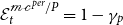 $\mathcal{E}_t^{\unicode{x1D4C2}\unicode{x1D4B8}^{per}/P} = 1-\gamma _p$
, and
 $\mathcal{E}_t^{\unicode{x1D4C2}\unicode{x1D4B8}^{per}/\unicode{x1D4C2}\unicode{x1D4B8}^{per}-} = \gamma _p$
. This leads to
 \begin{eqnarray*} \unicode{x1D4C2}\unicode{x1D4B8}_t^{per}: \quad\! \Delta \unicode{x1D4C2}_t^p \mathcal{E}_t^{Y/P}\! -\! 1 + \Upsilon _t\! &=& \beta \mathbb{E}_t \left ( \gamma _p \left(\Delta \unicode{x1D4C2}_{t+1}^p \mathcal{E}_{t+1}^{Y/P} - 1 + \Upsilon _{t+1}\right)\right.\\[5pt]&& \left. + \Delta \unicode{x1D4C2}_{t+1}^p \left(\mathcal{E}_{t+1}^{Y/P} -\nu _p\right) (1-\gamma _p) \right ) \\[5pt]&=& \beta \mathbb{E}_t \left ( \Delta \unicode{x1D4C2}_{t+1}^p \left(\mathcal{E}_{t+1}^{Y/P} -(1-\gamma _p) \nu _p\right) + \gamma _p (\Upsilon _{t+1} - 1) \right ) \end{eqnarray*}
A.2 Proofs
A.2.1 proof of the reminder
Reminder. In a New Keynesian model featuring monopolistic competition in both goods and labor markets, Rotemberg price adjustment costs, and an inflation-targeting monetary policy, the Ramsey allocation coincides with the first-best decentralized equilibrium at the zero-inflation steady-state, provided the following optimal labor subsidy is implemented
 \begin{equation*} \tau _l^{*,NK} = 1-\unicode{x1D4C2}^{p,NK} \unicode{x1D4C2}^{w,NK} \end{equation*}
where
 $\unicode{x1D4C2}^{p,NK} = \frac {\nu _p}{\nu _p-1}$
,
 $\unicode{x1D4C2}^{w,NK} = \frac {\nu _w}{\nu _w-1}$
,
 $\nu _p \gt 1$
, and
 $\nu _w \gt 1$
.
Proof. In an NK model with Rotemberg price-cost adjustments and inflation targeting, the optimal labor subsidy can be determined by solving the following Ramsey problem
 \begin{eqnarray*} \mathcal{L}_R^{NK} &=& \mathbb{E}_0 \sum _{t=0}^\infty \beta ^t \left ( \ln (C_t) - \frac {L_{t}^{1+\eta }}{1+\eta } \right ) \\ &&+ \lambda _{1,t} \left ( \frac {1}{C_t} -\mathbb{E}_t \frac {\pi _t^{\psi _\pi }}{\pi _{t+1} C_{t+1}} \right ) \\ &&+ \lambda _{2,t} \left ( A_t L_t - C_t \chi _t \right ) \end{eqnarray*}
where
 $\chi _t = (1 + \frac {\phi _p}{2} (\pi _t -1)^2)$
,
 $\Phi _{t;t+1} \triangleq \frac {1}{\unicode{x1D4C2}^{p,NK}} + \frac {\phi _p}{\nu _p} \left (\left (\pi _t -1\right ) \pi _t - \beta \mathbb{E}_t \left (\pi _{t+1} - 1 \right ) \pi _{t+1} \right )$
,
 $\unicode{x1D4C2}^{p,NK} = \frac {\nu _p}{\nu _p-1}$
,
 $\unicode{x1D4C2}^{w,NK} = \frac {\nu _w}{\nu _w-1}$
. In that problem
 $\tau _{l,t}$
will freely adjust, thereby rendering the condition,
 $\unicode{x1D4C2}^{w,NK} L_t^\eta C_t = A_t (1-\tau _{l,t}) \mathbb{E}_t \Phi _{t,t+1}$
, a non-binding constraint. The first-order conditions are (for
 $t\gt 0$
),
 \begin{eqnarray*} C_t: \quad \quad 0 &=& \frac {1}{C_t} - \lambda _{1,t} \frac {1}{C_{t}^2} + \lambda _{1,t-1} \mathbb{E}_{t-1} \beta ^{-1} \frac {\pi _{t-1}^{\psi _\pi }}{\pi _{t} C_{t}^2} - \lambda _{2,t} \chi _t \\ L_t: \quad \quad 0 &=& -L_t^\eta + \lambda _{2,t} A_t \\ \pi _t: \quad \quad 0 &=& -\lambda _{1,t} \mathbb{E}_t \frac {\psi _\pi \pi _t^{\psi _\pi -1}}{\pi _{t+1} C_{t+1}} + \lambda _{1,t-1} \mathbb{E}_{t-1} \beta ^{-1} \frac {\pi _{t-1}^{\psi _\pi }}{C_t \pi _{t}^2} -\lambda _{2,t} C_t \phi _p \left (\pi _t - 1 \right ) \end{eqnarray*}
Consider a zero-inflation steady-state,
 $\bar {\pi } = 1$
, and
 $\bar {A} = 1$
. Evidently,
 $\lambda _1 = 0$
, therefore,
 \begin{eqnarray*} \bar {C}: \quad \quad 0 &=& \frac {1}{\bar {C}} - \lambda _{2} \\ \bar {L}: \quad \quad \bar {L}^\eta &=& \lambda _{2} \end{eqnarray*}
consequently
 $\bar {L}^\eta \bar {C} = 1$
restores efficiency (first-best allocations, Blanchard and Galí (Reference Blanchard and Galí2007)). Now given that
 $\bar {L}^\eta \bar {C} = \frac {(1-\tau _{l})}{\unicode{x1D4C2}^{p,NK} \unicode{x1D4C2}^{w,NK}}$
at the zero-inflation steady-state, it follows that the optimal labor subsidy is
 \begin{eqnarray*} \frac {\left(1-\tau _{l}^{*,NK}\right)}{\unicode{x1D4C2}^{p,NK} \unicode{x1D4C2}^{w,NK}} &=& \bar {L}^\eta \bar {C} = 1, \\[3pt] \tau _{l}^{*,NK} &=& 1-\unicode{x1D4C2}^{p,NK} \unicode{x1D4C2}^{w,NK}, \end{eqnarray*}
A.2.2 Proposition 1
Proposition 1. In a fairness model with monopolistic competition in goods and labor markets, Rotemberg price adjustment costs, and an inflation-targeting monetary policy, the optimal labor subsidy at the zero-inflation steady-state is given by
 \begin{equation*} \tau _l^{*,F} = 1 - \left(1 - \Phi _\tau ^*\right)\, \bar {\unicode{x1D4C2}}^p\, \unicode{x1D4C2}^{w,NK} \end{equation*}
where the fairness-weight is
 \begin{equation*} \Phi _\tau ^* = - \bar {\mathcal{E}}^{F/\unicode{x1D4C2}^{per}} \cdot \frac {\left(1 - \bar {\mathcal{E}}^{\unicode{x1D4C2}\unicode{x1D4B8}^{per}/P}\right)(1 - \beta )}{\left(1 - \beta \bar {\mathcal{E}}^{\unicode{x1D4C2}\unicode{x1D4B8}^{per}/\unicode{x1D4C2}\unicode{x1D4B8}^{per,-}}\right)(1 - \beta \psi _\pi )} \quad \in (0,1) \end{equation*}
and the steady-state price markup is
 \begin{equation*} \bar {\unicode{x1D4C2}}^p = 1 + \frac {1}{(\nu _p - 1)\left ( 1 + \frac {(1 - \beta )\left(1 - \bar {\mathcal{E}}^{\unicode{x1D4C2}\unicode{x1D4B8}^{per}/P}\right)}{1 - \beta \bar {\mathcal{E}}^{\unicode{x1D4C2}\unicode{x1D4B8}^{per}/\unicode{x1D4C2}\unicode{x1D4B8}^{per,-}}} \cdot \bar {\mathcal{E}}^{F/\unicode{x1D4C2}^{per}} \right )} \end{equation*}
and
 $1 \lt \bar{\unicode{x1D4C2}}^{p} \lt \unicode{x1D4C2}^{p,NK}$
.
Proof. In the fairness model with Rotemberg price-cost adjustments and inflation targeting, the optimal subsidy can be determined by solving the following Ramsey problem

where
 $\mathcal{E}_t^{\unicode{x1D4C2}\unicode{x1D4B8}^{per}/.} = \mathcal{E}_t^{\unicode{x1D4C2}\unicode{x1D4B8}^{per}/P} \mathcal{E}_{t+1}^{\unicode{x1D4C2}\unicode{x1D4B8}^{per}/\unicode{x1D4C2}\unicode{x1D4B8}^{per}-} \left ( \mathcal{E}_{t+1}^{\unicode{x1D4C2}\unicode{x1D4B8}^{per}/P} \right )^{-1}$
,
 $\mathcal{E}_t^{F/\unicode{x1D4C2}^{per}} = -\frac {d \ln (F_t)}{d \ln (\unicode{x1D4C2}_t^{per})}$
. In that problem
 $\tau _{l,t}$
will freely adjust, thereby rendering the condition,
 $(1-\tau _{l,t}) w_t = L_t^\eta C_t \unicode{x1D4C2}^{w,NK}$
, a non-binding constraint. By homogeneity of degree 1 and the positivity of
 $ \mathbb{C}$
, and using the change of variables
 \begin{equation*} \pi _t = \frac {P_t}{P_{t-1}}, \quad m_{t-1}^{per} = \frac {P_{t-1}}{\unicode{x1D4C2}\unicode{x1D4B8}_{t-1}^{per}} \end{equation*}
one can rewrite
 \begin{equation*} \unicode{x1D4C2}_t^{per} = \frac {P_t}{\mathbb{C}\left(\omega _p P_t, \unicode{x1D4C2}\unicode{x1D4B8}_{t-1}^{per}\right)} = \frac {\pi _t P_{t-1}}{\mathbb{C}\left(\omega _p \pi _t P_{t-1}, \unicode{x1D4C2}\unicode{x1D4B8}_{t-1}^{per}\right)} \end{equation*}
This leads to the following composite mapping
 \begin{equation*} \widetilde {\mathbb{C}}\big(\pi _t, m_{t-1}^{per}\big) \triangleq \frac {\pi _t}{\mathbb{C}\left(\pi _t, \frac {1}{m_{t-1}^{per}}\right)} \quad \text{so that} \quad \unicode{x1D4C2}_t^{per} = \widetilde {\mathbb{C}}\big(\pi _t, m_{t-1}^{per}\big) \end{equation*}
since,
 \begin{equation*} \unicode{x1D4C2}\unicode{x1D4B8}_t^{per} = \frac {P_t}{\unicode{x1D4C2}_t^{per}} = \frac {P_t}{\widetilde {\mathbb{C}}\big(\pi _t, m_{t-1}^{per}\big)} \end{equation*}
so,
 \begin{align*} \frac {\partial \ln \big(\unicode{x1D4C2}\unicode{x1D4B8}_t^{per}\big)}{\partial \ln (P_t)} &= \frac {\partial }{\partial \ln (P_t)} \left ( \ln P_t - \ln \widetilde {\mathbb{C}}\big(\pi _t, m_{t-1}^{per}\big) \right ) \\[3pt] &= 1 - \frac {\partial \ln (\widetilde {\mathbb{C}})}{\partial \ln (\pi _t)} \cdot \frac {\partial \ln (\pi _t)}{\partial \ln (P_t)} = 1 - \mathcal{E}^{\widetilde {\mathbb{C}}}_{\pi _t} \end{align*}
similarly,
 \begin{align*} \frac {\partial \ln \big(\unicode{x1D4C2}\unicode{x1D4B8}_t^{per}\big)}{\partial \ln \big(\unicode{x1D4C2}\unicode{x1D4B8}_{t-1}^{per}\big)} &= - \frac {\partial \ln (\widetilde {\mathbb{C}})}{\partial \ln \big(m_{t-1}^{per}\big)} \cdot \frac {\partial \ln \big(m_{t-1}^{per}\big)}{\partial \ln \big(\unicode{x1D4C2}\unicode{x1D4B8}_{t-1}^{per}\big)} \\[3pt] &= - \frac {\partial \ln (\widetilde {\mathbb{C}})}{\partial \ln \big(m_{t-1}^{per}\big)} \cdot (-1) = \mathcal{E}^{\widetilde {\mathbb{C}}}_{m_{t-1}^{per}} \end{align*}
hence, the elasticity relations are
 \begin{equation*} \begin{aligned} &\mathcal{E}^{\unicode{x1D4C2}\unicode{x1D4B8}^{per}/P} = 1 - \mathcal{E}^{\unicode{x1D4C2}^{per}/\pi }, \\[3pt] &\mathcal{E}^{\unicode{x1D4C2}\unicode{x1D4B8}^{per}/\unicode{x1D4C2}\unicode{x1D4B8}^{per}-} = \mathcal{E}^{\unicode{x1D4C2}^{per}/\unicode{x1D4C2}^{per}} \end{aligned} \end{equation*}
The first-order conditions are (for
 $t\gt 0$
)
 \begin{eqnarray*} C_t: \quad \quad 0 &=& \frac {1}{C_t} - \lambda _{1,t} \frac {1}{C_{t}^2} + \lambda _{1,t-1} \mathbb{E}_{t-1} \beta ^{-1} \frac {\pi _{t-1}^{\psi _\pi }}{\pi _{t} C_{t}^2} - \lambda _{2,t} \chi _t \\[2pt] L_t: \quad \quad 0 &=& -L_t^\eta + \lambda _{2,t} A_t \\[2pt] \pi _t: \quad \quad 0 &=& -\lambda _{1,t} \mathbb{E}_t \frac {\psi _\pi \pi _t^{\psi _\pi -1}}{\pi _{t+1} C_{t+1}} + \lambda _{1,t-1} \mathbb{E}_{t-1} \beta ^{-1} \frac {\pi _{t-1}^{\psi _\pi }}{\pi _{t}^2 C_t} -\lambda _{2,t} C_t \phi _p \left (\pi _t - 1 \right ) - \lambda _{3,t} \frac {\partial \unicode{x1D4C2}_t^{per}}{\partial \pi _t} \\[2pt] &&- \lambda _{6,t} \phi _p (2 \pi _t - 1) + \lambda _{6,t-1} \mathbb{E}_{t-1} \phi _p (2 \pi _t -1) \\[2pt] F_t: \quad \quad 0 &=& \frac {1}{F_t} + \lambda _{4,t} \\[2pt] \unicode{x1D4C2}_t^{per}: \quad \quad 0 &=& \lambda _{3,t} - \beta \lambda _{3,t+1} \mathbb{E}_t \frac {\partial \unicode{x1D4C2}_{t+1}^{per}}{\partial \unicode{x1D4C2}_t^{per}} - \lambda _{4,t} \frac {d F_t}{d \unicode{x1D4C2}_t^{per}} \\[2pt] \unicode{x1D4C2}_t^p: \quad \quad 0 &=& \lambda _{5,t} \Big ( \mathcal{E}_{t}^{Y/P} + \Upsilon _t \\[2pt] &&- \Big ( 1 + \beta \mathbb{E}_t \Big ( \mathcal{E}_t^{\unicode{x1D4C2}\unicode{x1D4B8}^{per}/.} \Big(\Delta \unicode{x1D4C2}_{t+1}^p \mathcal{E}_{t+1}^{Y/P} - 1 + \Upsilon _{t+1}\Big)\! + \Delta \unicode{x1D4C2}_{t+1}^p \Big(\mathcal{E}_{t+1}^{Y/P} -\nu _p\Big) \mathcal{E}_t^{\unicode{x1D4C2}\unicode{x1D4B8}^{per}/P} \Big ) \Big ) \\[2pt] &&+ \lambda _{5,t-1} \mathbb{E}_{t-1} \unicode{x1D4C2}_{t-1}^p \Big(\mathcal{E}_{t-1}^{\unicode{x1D4C2}^{per}/.} \mathcal{E}_{t}^{Y/P} + \Big(\mathcal{E}_{t}^{Y/P} -\nu _p\Big) \mathcal{E}_{t-1}^{\unicode{x1D4C2}\unicode{x1D4B8}^{per}/P} \Big) \frac {1}{\big(\unicode{x1D4C2}_{t}^p\big)^2} + \lambda _{8,t} w_t \\[2pt] \mathcal{E}_t^{Y/P}: \quad \quad 0 &=& \lambda _{5,t} \big(\unicode{x1D4C2}_{t}^p-1\big) + \lambda _{5,t-1} \mathbb{E}_{t-1} \unicode{x1D4C2}_{t-1}^p \Delta \unicode{x1D4C2}_t^p \left ( \mathcal{E}_{t-1}^{\unicode{x1D4C2}^{per}/.} + \mathcal{E}_{t-1}^{\unicode{x1D4C2}\unicode{x1D4B8}^{per}/P} \right ) + \lambda _{7,t} \\[2pt] \Upsilon _t: \quad \quad 0 &=& \lambda _{5,t} \unicode{x1D4C2}_{t}^p - \lambda _{5,t-1} \mathbb{E}_{t-1} \unicode{x1D4C2}_{t-1}^p \mathcal{E}_{t-1}^{\unicode{x1D4C2}^{per}/.} + \lambda _{6,t} \\[2pt] w_t: \quad \quad 0 &=& \lambda _{8,t} \unicode{x1D4C2}_{t}^p \end{eqnarray*}
Consider a zero-inflation steady-state,
 $\bar {\pi } = 1$
and
 $\bar {A} = 1$
, therefore
 \begin{eqnarray*} \bar {C}: \quad \quad 0 &=& \frac {1}{\bar {C}} - \lambda _1 \frac {1}{\bar {C}^2} + \lambda _1 \beta ^{-1} \frac {1}{\bar {C}^2} - \lambda _2 \\[2pt] \bar {L}: \quad \quad 0 &=& -\bar {L}^\eta + \lambda _2 \\[2pt] \bar {\pi }: \quad \quad 0 &=& \lambda _1 \frac {1}{\bar {C}} \left ( \beta ^{-1} - \psi _\pi \right ) - \lambda _{3} \left . \frac {\partial \unicode{x1D4C2}_t^{per}}{\partial \pi _t} \right |_{\bar {\unicode{x1D4C2}}^{per}, \bar {\pi }} \\[2pt] \bar {F}: \quad \quad 0 &=& \frac {1}{\bar {F}} + \lambda _4 \\[2pt] \bar {\unicode{x1D4C2}}^{per}: \quad \quad 0 &=& \lambda _3 - \beta \lambda _{3} \left . \frac {\partial \unicode{x1D4C2}_{t+1}^{per}}{\partial \unicode{x1D4C2}_{t}^{per}} \right |_{\bar {\unicode{x1D4C2}}^{per}, \bar {\unicode{x1D4C2}}^{per}} -\lambda _4 \left . \frac {d F_t}{d \unicode{x1D4C2}_t^{per}} \right |_{\bar {F}, \bar {\unicode{x1D4C2}}^{per}} \\[2pt] \bar {\unicode{x1D4C2}}^p: \quad \quad 0 &=& \lambda _5 \Big ( \bar {\mathcal{E}}^{Y/P} - \Big ( 1 + \beta \Big ( \bar {\mathcal{E}}^{\unicode{x1D4C2}\unicode{x1D4B8}^{per}/.} \big(\Delta \bar {\unicode{x1D4C2}}^p \bar {\mathcal{E}}^{Y/P} - 1\big) + \Delta \bar {\unicode{x1D4C2}}^p \big(\bar {\mathcal{E}}^{Y/P} -\nu _p\big) \bar {\mathcal{E}}^{\unicode{x1D4C2}\unicode{x1D4B8}^{per}/P} \Big ) \Big ) \\[2pt] &&- \lambda _5 \left (\bar {\mathcal{E}}^{\unicode{x1D4C2}\unicode{x1D4B8}^{per}/.} \bar {\mathcal{E}}^{Y/P} + \big(\bar {\mathcal{E}}^{Y/P} -\nu _p\big) \bar {\mathcal{E}}^{\unicode{x1D4C2}\unicode{x1D4B8}^{per}/P} \right ) \frac {1}{\bar {\unicode{x1D4C2}}^{p}} +\lambda _8 \bar {w} \\[2pt] \bar {\mathcal{E}}: \quad \quad 0 &=& \lambda _5 (\bar {\unicode{x1D4C2}}^p-1) - \lambda _5 (\bar {\unicode{x1D4C2}}^p-1) \left ( \bar {\mathcal{E}}^{\unicode{x1D4C2}^{per}/.} + \bar {\mathcal{E}}^{\unicode{x1D4C2}\unicode{x1D4B8}^{per}/P} \right ) +\lambda _7 \\[2pt] \bar {\Upsilon }: \quad \quad 0 &=& \lambda _5 \bar {\unicode{x1D4C2}}^p \big(1 - \bar {\mathcal{E}}^{\unicode{x1D4C2}^{per}/.}\big) + \lambda _6 \\[2pt] \bar {w}: \quad \quad 0 &=& \lambda _8 \bar {\unicode{x1D4C2}}^p \end{eqnarray*}
Evidently,
 $\lambda _{5:8} = 0$
,
 \begin{eqnarray*} \bar {C}: \quad \quad 0 &=& \frac {1}{\bar {C}} - \lambda _1 \frac {1}{\bar {C}^2} + \lambda _1 \beta ^{-1} \frac {1}{\bar {C}^2} - \lambda _2 \\ \bar {L}: \quad \quad 0 &=& -\bar {L}^\eta + \lambda _2 \\ \bar {\pi }: \quad \quad 0 &=& \lambda _1 \frac {1}{\bar {C}} \left ( \beta ^{-1} - \psi _\pi \right ) + \frac { \left . \frac {1}{\bar {F}} \frac {d F_t}{d \unicode{x1D4C2}_t^{per}} \right | }{1 - \beta \left . \frac {\partial \unicode{x1D4C2}_{t+1}^{per}}{\partial \unicode{x1D4C2}_{t}^{per}} \right | } \cdot \left . \frac {\partial \unicode{x1D4C2}_t^{per}}{\partial \pi _t} \right | \end{eqnarray*}
and,
 \begin{eqnarray*} \bar {C}: \quad \quad 0 &=& 1 + \lambda _1 \frac {1}{\bar {C}} (\beta ^{-1} - 1) - \bar {L}^\eta \bar {C} \\ \bar {\pi }: \quad \quad 0 &=& \lambda _1 \frac {1}{\bar {C}} \left ( \beta ^{-1} - \psi _\pi \right ) - \frac { \bar {\mathcal{E}}^{F/\unicode{x1D4C2}^{per}} \cdot \bar {\mathcal{E}}^{\unicode{x1D4C2}^{per}/\pi } }{1 - \beta \bar {\mathcal{E}}^{\unicode{x1D4C2}^{per}/\unicode{x1D4C2}^{per\,-}}} \end{eqnarray*}
consequently,
 \begin{eqnarray*} \bar {L}^\eta \bar {C} &=& 1 + \bar {\mathcal{E}}^{F/\unicode{x1D4C2}^{per}} \cdot \frac {\bar {\mathcal{E}}^{\unicode{x1D4C2}^{per}/\pi } (\beta ^{-1}-1)}{\big(1 - \beta \bar {\mathcal{E}}^{\unicode{x1D4C2}^{per}/\unicode{x1D4C2}^{per\,-}}\big) (\beta ^{-1} - \psi _\pi )}\\ &=& 1 + \bar {\mathcal{E}}^{F/\unicode{x1D4C2}^{per}} \cdot \frac {\bar {\mathcal{E}}^{\unicode{x1D4C2}^{per}/\pi } (1-\beta )}{(1 - \beta \bar {\mathcal{E}}^{\unicode{x1D4C2}^{per}/\unicode{x1D4C2}^{per\,-}}) (1 - \beta \psi _\pi )} \end{eqnarray*}
given the equivalence in elasticities demonstrated above,
 \begin{eqnarray*} \bar {L}^\eta \bar {C} &=& 1 + \bar {\mathcal{E}}^{F/\unicode{x1D4C2}^{per}} \frac {\big( 1- \bar {\mathcal{E}}^{\unicode{x1D4C2}\unicode{x1D4B8}^{per}/P} \big) (1-\beta )}{\big(1 - \beta \bar {\mathcal{E}}^{\unicode{x1D4C2}\unicode{x1D4B8}^{per}/\unicode{x1D4C2}\unicode{x1D4B8}^{per\,-}}\big) (1 - \beta \psi _\pi )} \end{eqnarray*}
Now given that
 $\bar {L}^\eta \bar {C} = \frac {1-\tau _{l}}{\unicode{x1D4C2}^{w,NK} \bar {\unicode{x1D4C2}}^p}$
at the steady-state of the competitive equilibrium, it follows that the optimal fiscal policy is
 \begin{eqnarray*} \tau _l^{*,F} &=& 1 - \left ( 1 + \bar {\mathcal{E}}^{F/\unicode{x1D4C2}^{per}} \frac {\big( 1- \bar {\mathcal{E}}^{\unicode{x1D4C2}\unicode{x1D4B8}^{per}/P} \big) (1-\beta )}{\big(1 - \beta \bar {\mathcal{E}}^{\unicode{x1D4C2}\unicode{x1D4B8}^{per}/\unicode{x1D4C2}\unicode{x1D4B8}^{per\,-}}\big) (1 - \beta \psi _\pi )} \right ) \bar{\unicode{x1D4C2}}^{p} \unicode{x1D4C2}^{w,NK} \\ &=& 1 - \big(1-\Phi _\tau ^{*}\big) \bar{\unicode{x1D4C2}}^{p} \unicode{x1D4C2}^{w,NK}, \quad \end{eqnarray*}
where
 $\Phi _\tau ^{*} = - \bar {\mathcal{E}}^{F/\unicode{x1D4C2}^{per}} \frac {\big( 1- \bar {\mathcal{E}}^{\unicode{x1D4C2}\unicode{x1D4B8}^{per}/P} \big) (1-\beta )}{(1 - \beta \bar {\mathcal{E}}^{\unicode{x1D4C2}\unicode{x1D4B8}^{per}/\unicode{x1D4C2}\unicode{x1D4B8}^{per\,-}}) (1 - \beta \psi _\pi )}$
Sub-proposition 1.
Under the model assumptions, the fairness-weight term
 $\Phi _\tau ^*$
lies strictly between zero and one, i.e.,
 \begin{equation*} \Phi _\tau ^* \in (0,1) \end{equation*}
which guarantees strictly positive steady-state allocations
 $(\bar {L}, \bar {C}, \bar {Y}) \gt 0$
. This holds provided the following restriction on the steady-state elasticity of the fairness function
 $\mathbb{F}$
is satisfied
 \begin{equation*} - \frac {\mathbb{F}'(\bar {\unicode{x1D4C2}}^{per}) \cdot \bar {\unicode{x1D4C2}}^{per}}{\mathbb{F}(\bar {\unicode{x1D4C2}}^{per})} \lt \frac {\big(1 - \beta \bar {\mathcal{E}}^{\unicode{x1D4C2}\unicode{x1D4B8}^{per}/\unicode{x1D4C2}\unicode{x1D4B8}^{per,-}}\big)(1 - \beta \psi _\pi )}{\big(1 - \bar {\mathcal{E}}^{\unicode{x1D4C2}\unicode{x1D4B8}^{per}/P}\big)(1 - \beta )} \end{equation*}
This condition restricts the shape (elasticity) of the fairness function
 $\mathbb{F}$
around the steady-state to ensure positive allocations.
Proof. The steady-state labor allocation is given by
 \begin{equation*} \bar {L} = \left ( \frac {1 - \tau _l^{*,F}}{\bar {\unicode{x1D4C2}}^{p} \unicode{x1D4C2}^{w,NK}} \right )^{\frac {1}{1+\eta }} = \big(1 - \Phi _\tau ^*\big)^{\frac {1}{1+\eta }} \end{equation*}
and positivity of allocations requires
 $0 \lt \Phi _\tau ^* \lt 1$
.
The fairness-weight term
 $\Phi _\tau ^*$
is defined as
 \begin{equation*} \Phi _\tau ^{*} = -\bar {\mathcal{E}}^{F/\unicode{x1D4C2}^{per}} \cdot \frac {\big(1 - \bar {\mathcal{E}}^{\unicode{x1D4C2}\unicode{x1D4B8}^{per}/P}\big)(1 - \beta )}{(1 - \beta \bar {\mathcal{E}}^{\unicode{x1D4C2}\unicode{x1D4B8}^{per}/\unicode{x1D4C2}\unicode{x1D4B8}^{per,-}})(1 - \beta \psi _\pi )} \end{equation*}
where
 \begin{equation*} \bar {\mathcal{E}}^{F/\unicode{x1D4C2}^{per}} = -\left . \frac {d F_t}{d \unicode{x1D4C2}_t^{per}} \cdot \frac {\unicode{x1D4C2}_t^{per}}{F_t} \right |_{\bar {F}, \bar {\unicode{x1D4C2}}^{per}} = -\frac {\mathbb{F}'(\bar {\unicode{x1D4C2}}^{per}) \cdot \bar {\unicode{x1D4C2}}^{per}}{\mathbb{F}(\bar {\unicode{x1D4C2}}^{per})} \gt 0 \end{equation*}
due to
 $\mathbb{F}$
being strictly positive and strictly decreasing. From the properties of the inference function
 $\mathbb{C}$
, the elasticities satisfy
 \begin{equation*} \bar {\mathcal{E}}^{\unicode{x1D4C2}\unicode{x1D4B8}^{per}/P} \in (0,1), \quad \bar {\mathcal{E}}^{\unicode{x1D4C2}\unicode{x1D4B8}^{per}/\unicode{x1D4C2}\unicode{x1D4B8}^{per,-}} \in (0,1) \end{equation*}
and under standard parameter values,
 \begin{equation*} \beta \in (0,1), \quad \psi _\pi \geq 1.5, \quad 1 - \beta \psi _\pi \lt 0 \end{equation*}
Analyzing signs
-
•
 $\bar {\mathcal{E}}^{F/\unicode{x1D4C2}^{per}} \gt 0$
by definition,
-
• The numerator
$\big(1 - \bar {\mathcal{E}}^{\unicode{x1D4C2}\unicode{x1D4B8}^{per}/P}\big)(1 - \beta ) \gt 0$
, -
• The denominator
$(1 - \beta \bar {\mathcal{E}}^{\unicode{x1D4C2}\unicode{x1D4B8}^{per}/\unicode{x1D4C2}\unicode{x1D4B8}^{per,-}})(1 - \beta \psi _\pi ) \lt 0$
.


Therefore,
 $\Phi _\tau ^* \gt 0$
.
To ensure
 $\Phi _\tau ^* \lt 1$
, the following inequality must hold
 \begin{equation} - \frac {\mathbb{F}'(\bar {\unicode{x1D4C2}}^{per}) \cdot \bar {\unicode{x1D4C2}}^{per}}{\mathbb{F}(\bar {\unicode{x1D4C2}}^{per})} \lt \frac {\big(1 - \beta \bar {\mathcal{E}}^{\unicode{x1D4C2}\unicode{x1D4B8}^{per}/\unicode{x1D4C2}\unicode{x1D4B8}^{per,-}}\big)(1 - \beta \psi _\pi )}{\big(1 - \bar {\mathcal{E}}^{\unicode{x1D4C2}\unicode{x1D4B8}^{per}/P}\big)(1 - \beta )} \end{equation}
which restricts the elasticity of the fairness function
 $\mathbb{F}$
around the steady-state.
Under this condition, the fairness-weight satisfies
 \begin{equation*} \Phi _\tau ^* \in (0,1) \end{equation*}
ensuring strictly positive steady-state allocations
 $\bar {L} = (1 - \Phi _\tau ^*)^{\frac {1}{1+\eta }} \gt 0$
.
The steady-state of the price elasticity of demand is
 \begin{eqnarray*} \bar {\mathcal{E}}^{Y/P} = \nu _p + (\nu _p-1) \bar {\mathcal{E}}^{F/\unicode{x1D4C2}^{per}} \big( 1- \bar {\mathcal{E}}^{\unicode{x1D4C2}\unicode{x1D4B8}^{per}/P} \big) = \nu _p + (\nu _p-1) \bar {\mathcal{E}}^{F/\unicode{x1D4C2}^{per}} \bar {\mathcal{E}}^{\unicode{x1D4C2}\unicode{x1D4B8}^{per}/\unicode{x1D4C2}\unicode{x1D4B8}^{per}-} \end{eqnarray*}
given that
 $\bar {\mathcal{E}}^{\unicode{x1D4C2}\unicode{x1D4B8}^{per}/\unicode{x1D4C2}\unicode{x1D4B8}^{per}-} + \bar {\mathcal{E}}^{\unicode{x1D4C2}\unicode{x1D4B8}^{per}/P} = 1$
. The steady-state of the price markup is
 \begin{eqnarray*} &&\Delta \bar{\unicode{x1D4C2}}^p \bar {\mathcal{E}}^{Y/P} = 1 + \beta \big( \bar {\mathcal{E}}^{\unicode{x1D4C2}\unicode{x1D4B8}^{per}/\unicode{x1D4C2}\unicode{x1D4B8}^{per}-} \big(\Delta \bar{\unicode{x1D4C2}}^p \bar {\mathcal{E}}^{Y/P} - 1\big)\\&&\quad\qquad\qquad + \Delta \bar{\unicode{x1D4C2}}^p \big( \bar {\mathcal{E}}^{Y/P} - \nu _p \big) \big( 1 - \bar {\mathcal{E}}^{\unicode{x1D4C2}\unicode{x1D4B8}^{per}/\unicode{x1D4C2}\unicode{x1D4B8}^{per}-} \big) \big) \\ &&\bar{\unicode{x1D4C2}}^p = \frac { \bar {\mathcal{E}}^{Y/P} (1-\beta ) + \beta \nu _p \bar {\mathcal{E}}^{\unicode{x1D4C2}\unicode{x1D4B8}^{per}/\unicode{x1D4C2}\unicode{x1D4B8}^{per}-}}{\bar {\mathcal{E}}^{Y/P} (1-\beta ) + \beta \nu _p \bar {\mathcal{E}}^{\unicode{x1D4C2}\unicode{x1D4B8}^{per}/\unicode{x1D4C2}\unicode{x1D4B8}^{per}-} - \big(1-\beta \bar {\mathcal{E}}^{\unicode{x1D4C2}\unicode{x1D4B8}^{per}/\unicode{x1D4C2}\unicode{x1D4B8}^{per}-}\big)} \\ &&\bar{\unicode{x1D4C2}}^p = 1 + \frac {1-\beta \bar {\mathcal{E}}^{\unicode{x1D4C2}\unicode{x1D4B8}^{per}/\unicode{x1D4C2}\unicode{x1D4B8}^{per}}}{{\big(\nu _p + (\nu _p-1) \bar {\mathcal{E}}^{F/\unicode{x1D4C2}^{per}} \bar {\mathcal{E}}^{\unicode{x1D4C2}\unicode{x1D4B8}^{per}/\unicode{x1D4C2}\unicode{x1D4B8}^{per}-} \big) (1-\beta ) + \beta \nu _p \bar {\mathcal{E}}^{\unicode{x1D4C2}\unicode{x1D4B8}^{per}/\unicode{x1D4C2}\unicode{x1D4B8}^{per}-}}} \\&& \qquad\qquad\qquad\qquad\qquad\qquad\qquad\qquad\qquad\qquad\qquad\qquad { - (1-\beta \bar {\mathcal{E}}^{\unicode{x1D4C2}\unicode{x1D4B8}^{per}/\unicode{x1D4C2}\unicode{x1D4B8}^{per}-})}\\&&\bar{\unicode{x1D4C2}}^p = 1 + \frac {1-\beta \bar {\mathcal{E}}^{\unicode{x1D4C2}\unicode{x1D4B8}^{per}/\unicode{x1D4C2}\unicode{x1D4B8}^{per}-}}{(\nu _p-1) \left ( (1-\beta \bar {\mathcal{E}}^{\unicode{x1D4C2}\unicode{x1D4B8}^{per}/\unicode{x1D4C2}\unicode{x1D4B8}^{per}}) + (1-\beta ) \left ( 1 - \bar {\mathcal{E}}^{\unicode{x1D4C2}\unicode{x1D4B8}^{per}/\unicode{x1D4C2}\unicode{x1D4B8}^{per}-} \right ) \bar {\mathcal{E}}^{F/\unicode{x1D4C2}^{per}} \right )} \\ &&\bar{\unicode{x1D4C2}}^p = 1 + \frac {1}{(\nu _p-1) \left ( 1 + \frac {(1-\beta ) \bar {\mathcal{E}}^{\unicode{x1D4C2}^{per}/\unicode{x1D4C2}\unicode{x1D4B8}^{per}-}}{1-\beta \bar {\mathcal{E}}^{\unicode{x1D4C2}^{per}/\unicode{x1D4C2}^{per}-}} \cdot \bar {\mathcal{E}}^{F/\unicode{x1D4C2}^{per}} \right )} \\ \Longleftrightarrow &&\bar{\unicode{x1D4C2}}^p = 1 + \frac {1}{(\nu _p-1) \left ( 1 + \frac {(1-\beta ) \big(1-\bar {\mathcal{E}}^{\unicode{x1D4C2}^{per}/P} \big)}{1-\beta \bar {\mathcal{E}}^{\unicode{x1D4C2}^{per}/\unicode{x1D4C2}^{per}-}} \cdot \bar {\mathcal{E}}^{F/\unicode{x1D4C2}^{per}} \right )} \\ \end{eqnarray*}
Sub-proposition 2. The steady-state price markup in the fairness model satisfies
 \begin{equation*} 1 \lt \bar {\unicode{x1D4C2}}^p \lt \unicode{x1D4C2}^{p,NK} = 1 + \frac {1}{\nu _p - 1} \end{equation*}
Proof. The modified markup expression is given by
 \begin{equation*} \bar {\unicode{x1D4C2}}^p = 1 + \frac {1}{(\nu _p - 1)\Theta _m}, \quad \text{where} \quad \Theta _m = \left ( 1 + \frac {(1 - \beta )\big(1 - \bar {\mathcal{E}}^{\unicode{x1D4C2}\unicode{x1D4B8}^{per}/P}\big)}{1 - \beta \bar {\mathcal{E}}^{\unicode{x1D4C2}\unicode{x1D4B8}^{per}/\unicode{x1D4C2}\unicode{x1D4B8}^{per}-}} \cdot \bar {\mathcal{E}}^{F/\unicode{x1D4C2}^{per}} \right ) \end{equation*}
Given that
 \begin{equation*} \bar {\mathcal{E}}^{\unicode{x1D4C2}\unicode{x1D4B8}^{per}/P} \in (0,1), \quad \bar {\mathcal{E}}^{\unicode{x1D4C2}\unicode{x1D4B8}^{per}/\unicode{x1D4C2}\unicode{x1D4B8}^{per}-} \in (0,1), \quad \beta \in (0,1), \quad \bar {\mathcal{E}}^{F/\unicode{x1D4C2}^{per}} \gt 0 \end{equation*}
it follows that the multiplicative term in
 $\Theta _m$
is strictly positive. Hence,
 \begin{equation*} \Theta _m \gt 1 \end{equation*}
This implies
 \begin{equation*} \frac {1}{(\nu _p - 1)\Theta _m} \lt \frac {1}{\nu _p - 1} \quad \Rightarrow \quad 1 \lt \bar {\unicode{x1D4C2}}^p \lt 1 + \frac {1}{\nu _p - 1} = \unicode{x1D4C2}^{p,NK} \end{equation*}
as desired.
A.2.3 Corollary 1
Corollary 1.
Because
 $\tau _l^{*,F} \gt \tau _l^{*,NK}$
, the optimal labor policy in the fairness model cannot restore the first-best allocation.
Proof. From Proposition1, the Ramsey planner in the standard New Keynesian model restores the first-best allocation by setting the labor subsidy
 \begin{equation*} \tau _l^{*,NK} = 1 - \unicode{x1D4C2}^{w,NK} \unicode{x1D4C2}^{p,NK}, \quad \mathrm{with} \quad \unicode{x1D4C2}^{p,NK} = 1 + \frac {1}{\nu _p - 1} \end{equation*}
In the fairness model, the optimal fiscal policy is
 \begin{equation*} \tau _l^{*,F} = 1 - \big(1 - \Phi _\tau ^*\big) \bar {\unicode{x1D4C2}}^p \unicode{x1D4C2}^{w,NK}, \quad \text{where} \quad \Phi _\tau ^* \in (0,1) \quad \text{(sub-proposition 1)} \end{equation*}
From the sub-proposition 2
 \begin{equation*} 1 \lt \bar {\unicode{x1D4C2}}^p \lt \unicode{x1D4C2}^{p,NK} \end{equation*}
which implies
 \begin{equation*} \big(1 - \Phi _\tau ^*\big) \bar {\unicode{x1D4C2}}^p \lt \unicode{x1D4C2}^{p,NK} \quad \Rightarrow \quad \tau _l^{*,F} \gt \tau _l^{*,NK} \end{equation*}
as desired.
This strict inequality in subsidies implies a wedge that cannot be fully offset under perceived fairness dynamics. As a result, the first-best allocation
 $\bar {L}^{NK} = 1$
is no longer attainable. In particular, under the fairness model, the steady-state labor allocation becomes
 \begin{equation*} \bar {L} = \left ( \frac {1 - \tau _l^{*,F}}{\bar {\unicode{x1D4C2}}^p \unicode{x1D4C2}^{w,NK}} \right )^{\frac {1}{1+\eta }} = \left ( 1 - \Phi _\tau ^* \right )^{\frac {1}{1+\eta }} \lt 1 = \bar {L}^{NK} \end{equation*}
Therefore, the planner cannot restore the first-best allocation in the presence of fairness preferences.
A.2.4 Corollary 2
Corollary 2.
The optimal policy may be a labor tax,
 $\tau _l^{*,F} \gt 0$
, rather than a labor subsidy.
Proof. The optimal fiscal policy in the fairness model is given by
 \begin{equation*} \tau _l^{*,F} = 1 - \big(1 - \Phi _\tau ^*\big) \bar {\unicode{x1D4C2}}^p \unicode{x1D4C2}^{w,NK} \end{equation*}
Suppose
 $\unicode{x1D4C2}^{w,NK} = 1$
(without loss of generality). Then the condition for a positive labor tax simplifies to
 \begin{equation*} \big(1 - \Phi _\tau ^*\big) \bar {\unicode{x1D4C2}}^p \lt 1 \quad \Rightarrow \quad \tau _l^{*,F} \gt 0, \quad \end{equation*}
In the limit as
 $\Phi _\tau ^* \rightarrow 1$
, then
 \begin{equation*} \tau _l^{*,F} \rightarrow 1 \end{equation*}
Let
 $\mathbb{T}$
be a function
 \begin{align*} \mathbb{T}\left (\bar {\mathcal{E}}^{\unicode{x1D4C2}\unicode{x1D4B8}^{per}/P},\bar {\mathcal{E}}^{\unicode{x1D4C2}\unicode{x1D4B8}^{per}/\unicode{x1D4C2}\unicode{x1D4B8}^{per}-},\bar {\mathcal{E}}^{F/\unicode{x1D4C2}^{per}},\nu _p,\psi _\pi \right ) & = \big(1 - \Phi _\tau ^*\big) \bar {\unicode{x1D4C2}}^p\\& = \left (1 - \Phi _\tau ^* \right ) \left (1 + \frac {1}{(\nu _p - 1)(1 + \mathcal{A})} \right ) \end{align*}
where the auxiliary term
 $\mathcal{A}$
is
 \begin{equation*} \mathcal{A} = \frac {(1 - \beta )\big(1 - \bar {\mathcal{E}}^{\unicode{x1D4C2}\unicode{x1D4B8}^{per}/P}\big)}{1 - \beta \bar {\mathcal{E}}^{\unicode{x1D4C2}\unicode{x1D4B8}^{per}/\unicode{x1D4C2}\unicode{x1D4B8}^{per}-}} \cdot \bar {\mathcal{E}}^{F/\unicode{x1D4C2}^{per}} \end{equation*}
Partial derivatives of
 $\mathcal{A}$
 \begin{align*} \frac {\partial \mathcal{A}}{\partial \bar {\mathcal{E}}^{\unicode{x1D4C2}\unicode{x1D4B8}^{per}/\unicode{x1D4C2}\unicode{x1D4B8}^{per}-}} &= \frac {(1 - \beta )\big(1 - \bar {\mathcal{E}}^{\unicode{x1D4C2}\unicode{x1D4B8}^{per}/P}\big) \beta \bar {\mathcal{E}}^{F/\unicode{x1D4C2}^{per}}}{\left (1 - \beta \bar {\mathcal{E}}^{\unicode{x1D4C2}\unicode{x1D4B8}^{per}/\unicode{x1D4C2}\unicode{x1D4B8}^{per}-}\right )^2} \gt 0 \\ \frac {\partial \mathcal{A}}{\partial \bar {\mathcal{E}}^{F/\unicode{x1D4C2}^{per}}} &= \frac {(1 - \beta )\big(1 - \bar {\mathcal{E}}^{\unicode{x1D4C2}\unicode{x1D4B8}^{per}/P}\big)}{1 - \beta \bar {\mathcal{E}}^{\unicode{x1D4C2}\unicode{x1D4B8}^{per}/\unicode{x1D4C2}\unicode{x1D4B8}^{per}-}} \gt 0 \\ \frac {\partial \mathcal{A}}{\partial \bar {\mathcal{E}}^{\unicode{x1D4C2}\unicode{x1D4B8}^{per}/P}} &= -\frac {(1 - \beta ) \bar {\mathcal{E}}^{F/\unicode{x1D4C2}^{per}}}{1 - \beta \bar {\mathcal{E}}^{\unicode{x1D4C2}\unicode{x1D4B8}^{per}/\unicode{x1D4C2}\unicode{x1D4B8}^{per}-}} \lt 0 \end{align*}
Partial derivatives of
 $\bar {\unicode{x1D4C2}}^p = 1 + \frac {1}{(\nu _p - 1)(1 + \mathcal{A})}$
 \begin{align*} \frac {\partial \bar {\unicode{x1D4C2}}^p}{\partial \bar {\mathcal{E}}^{\unicode{x1D4C2}\unicode{x1D4B8}^{per}/\unicode{x1D4C2}\unicode{x1D4B8}^{per}-}} &= -\frac {1}{(\nu _p - 1)(1 + \mathcal{A})^2} \cdot \frac {\partial \mathcal{A}}{\partial \bar {\mathcal{E}}^{\unicode{x1D4C2}\unicode{x1D4B8}^{per}/\unicode{x1D4C2}\unicode{x1D4B8}^{per}-}} \lt 0 \\ \frac {\partial \bar {\unicode{x1D4C2}}^p}{\partial \bar {\mathcal{E}}^{F/\unicode{x1D4C2}^{per}}} &= -\frac {1}{(\nu _p - 1)(1 + \mathcal{A})^2} \cdot \frac {\partial \mathcal{A}}{\partial \bar {\mathcal{E}}^{F/\unicode{x1D4C2}^{per}}} \lt 0 \\ \frac {\partial \bar {\unicode{x1D4C2}}^p}{\partial \bar {\mathcal{E}}^{\unicode{x1D4C2}\unicode{x1D4B8}^{per}/P}} &= -\frac {1}{(\nu _p - 1)(1 + \mathcal{A})^2} \cdot \frac {\partial \mathcal{A}}{\partial \bar {\mathcal{E}}^{\unicode{x1D4C2}\unicode{x1D4B8}^{per}/P}} \gt 0 \\ \frac {\partial \bar {\unicode{x1D4C2}}^p}{\partial \nu _p} &= - \frac {1}{(\nu _p - 1)^2 (1 + \mathcal{A})} \lt 0 \end{align*}
Partial derivatives of
 $\Phi _\tau ^{*} = - \frac {\mathcal{A}}{1 - \beta \psi _\pi }$
 \begin{align*} \frac {\partial \Phi _\tau ^{*}}{\partial \bar {\mathcal{E}}^{\unicode{x1D4C2}\unicode{x1D4B8}^{per}/\unicode{x1D4C2}\unicode{x1D4B8}^{per}-}} &= - \frac {1}{1 - \beta \psi _\pi } \cdot \frac {\partial \mathcal{A}}{\partial \bar {\mathcal{E}}^{\unicode{x1D4C2}\unicode{x1D4B8}^{per}/\unicode{x1D4C2}\unicode{x1D4B8}^{per}-}} \gt 0 \\ \frac {\partial \Phi _\tau ^{*}}{\partial \bar {\mathcal{E}}^{F/\unicode{x1D4C2}^{per}}} &= - \frac {1}{1 - \beta \psi _\pi } \cdot \frac {\partial \mathcal{A}}{\partial \bar {\mathcal{E}}^{F/\unicode{x1D4C2}^{per}}} \gt 0 \\ \frac {\partial \Phi _\tau ^{*}}{\partial \bar {\mathcal{E}}^{\unicode{x1D4C2}\unicode{x1D4B8}^{per}/P}} &= - \frac {1}{1 - \beta \psi _\pi } \cdot \frac {\partial \mathcal{A}}{\partial \bar {\mathcal{E}}^{\unicode{x1D4C2}\unicode{x1D4B8}^{per}/P}} \lt 0 \\ \frac {\partial \Phi _\tau ^{*}}{\partial \psi _\pi } &= - \mathcal{A} \cdot \frac {\beta }{(1 - \beta \psi _\pi )^2} \lt 0 \end{align*}
Partial derivatives of
 $\mathbb{T}$
 \begin{align*} \frac {\partial \mathbb{T}}{\partial \bar {\mathcal{E}}^{\unicode{x1D4C2}\unicode{x1D4B8}^{per}/\unicode{x1D4C2}\unicode{x1D4B8}^{per}-}} &= -\frac {\partial \Phi _\tau ^*}{\partial \bar {\mathcal{E}}^{\unicode{x1D4C2}\unicode{x1D4B8}^{per}/\unicode{x1D4C2}\unicode{x1D4B8}^{per}-}} \left (1 + \frac {1}{(\nu _p - 1)(1 + \mathcal{A})} \right )\\& \quad - \frac {\big(1 - \Phi _\tau ^*\big)}{(\nu _p - 1)(1 + \mathcal{A})^2} \cdot \frac {\partial \mathcal{A}}{\partial \bar {\mathcal{E}}^{\unicode{x1D4C2}\unicode{x1D4B8}^{per}/\unicode{x1D4C2}\unicode{x1D4B8}^{per}-}} \lt 0 \\ \frac {\partial \mathbb{T}}{\partial \bar {\mathcal{E}}^{F/\unicode{x1D4C2}^{per}}} &= -\frac {\partial \Phi _\tau ^*}{\partial \bar {\mathcal{E}}^{F/\unicode{x1D4C2}^{per}}} \left (1 + \frac {1}{(\nu _p - 1)(1 + \mathcal{A})} \right ) - \frac {\big(1 - \Phi _\tau ^*\big)}{(\nu _p - 1)(1 + \mathcal{A})^2} \cdot \frac {\partial \mathcal{A}}{\partial \bar {\mathcal{E}}^{F/\unicode{x1D4C2}^{per}}} \lt 0 \\ \frac {\partial \mathbb{T}}{\partial \bar {\mathcal{E}}^{\unicode{x1D4C2}\unicode{x1D4B8}^{per}/P}} &= -\frac {\partial \Phi _\tau ^*}{\partial \bar {\mathcal{E}}^{\unicode{x1D4C2}\unicode{x1D4B8}^{per}/P}} \left (1 + \frac {1}{(\nu _p - 1)(1 + \mathcal{A})} \right ) - \frac {\big(1 - \Phi _\tau ^*\big)}{(\nu _p - 1)(1 + \mathcal{A})^2} \cdot \frac {\partial \mathcal{A}}{\partial \bar {\mathcal{E}}^{\unicode{x1D4C2}\unicode{x1D4B8}^{per}/P}} \gt 0 \\ \frac {\partial \mathbb{T}}{\partial \psi _\pi } &= -\frac {\partial \Phi _\tau ^*}{\partial \psi _\pi } \left (1 + \frac {1}{(\nu _p - 1)(1 + \mathcal{A})} \right ) \gt 0 \\ \frac {\partial \mathbb{T}}{\partial \nu _p} &= - \frac {\big(1 - \Phi _\tau ^*\big)}{(\nu _p - 1)^2(1 + \mathcal{A})} \lt 0 \end{align*}
Consequently
 \begin{equation*} \boxed{{ \frac {\partial \tau _l^{*,F}}{\partial \bar {\mathcal{E}}^{\unicode{x1D4C2}\unicode{x1D4B8}^{per}/\unicode{x1D4C2}\unicode{x1D4B8}^{per}-}} \gt 0, \quad \frac {\partial \tau _l^{*,F}}{\partial \bar {\mathcal{E}}^{F/\unicode{x1D4C2}\unicode{x1D4B8}^{per}}} \gt 0, \quad \frac {\partial \tau _l^{*,F}}{\partial \nu _p} \gt 0, \quad \frac {\partial \tau _l^{*,F}}{\partial \bar {\mathcal{E}}^{\unicode{x1D4C2}\unicode{x1D4B8}^{per}/P}} \lt 0, \quad \frac {\partial \tau _l^{*,F}}{\partial \psi _\pi } \lt 0 }} \end{equation*}
Sub-Corollary to Corollaries 1 and 2: Welfare consequences of the optimal fiscal policy.
Define household welfare recursively as the expected discounted sum of period utility,
 \begin{equation*} \mathcal{W}_t = \mathcal{U}_t + \beta \mathbb{E}_t \mathcal{W}_{t+1} \end{equation*}
with period utility
 $\mathcal{U}_t = \ln (\mathcal{C}_t) - \frac {L_t^{1+\eta }}{1+\eta }$
. At the zero-inflation steady-state with
 $\bar {F} = 1$
, consumption equals labor,
 $\bar {\mathcal{C}} = \bar {L}$
, so steady-state welfare becomes
 \begin{equation*} \bar {\mathcal{W}} = \frac {\ln (\bar {L}) - \frac {\bar {L}^{1+\eta }}{1+\eta }}{1 - \beta } \end{equation*}
Assume
 $\bar {L} \gt 0$
,
 $\beta = 0.99$
,
 $\eta \gt 1$
,
 $\unicode{x1D4C2}^{w,NK} \gt 1$
, and
 $\bar {\unicode{x1D4C2}}^p \gt 1$
. Denote by
 $\bar {\mathcal{W}}^{F,N}$
the welfare under fairness without intervention, and
 $\bar {\mathcal{W}}^{F,\tau _l^*}$
the welfare under the optimal fiscal policy
 $\tau _l^{*,F}$
.
Without intervention
 \begin{equation*} \bar {L}^{F,N} = \left ( \frac {1}{\unicode{x1D4C2}^{w,NK} \bar {\unicode{x1D4C2}}^p} \right )^{\frac {1}{1+\eta }} \in (0,1) \end{equation*}
With an optimal policy
 $\tau _l^{*,F}$
 \begin{equation*} \bar {L}^{F,\tau _l^*} = \left ( \frac {1 - \tau _l^{*,F}}{\unicode{x1D4C2}^{w,NK} \bar {\unicode{x1D4C2}}^p} \right )^{\frac {1}{1+\eta }} = \left (1 - \Phi _\tau ^*\right )^{\frac {1}{1+\eta }} \end{equation*}
Two cases
-
1.
$\tau _l^{*,F} \gt 0$
(a tax)
$\Longleftrightarrow$
$(1 - \Phi _\tau ^*) \bar {\unicode{x1D4C2}}^p \unicode{x1D4C2}^{w,NK} \lt 1$
-
2.
$\tau _l^{*,F} \lt 0$
(a subsidy)
$\Longleftrightarrow$
$(1 - \Phi _\tau ^*) \bar {\unicode{x1D4C2}}^p \unicode{x1D4C2}^{w,NK} \gt 1$


Over
 $\bar {L} \in (0,1)$
, the welfare function satisfies
 \begin{equation*} \frac {d\bar {\mathcal{W}}}{d\bar {L}} = \frac {1}{1 - \beta } \left (\frac {1}{\bar {L}} - \bar {L}^\eta \right ) \gt 0 \end{equation*}
Thus, welfare increases in labor.
- Case 1: Tax (
 $\tau _l^{*,F} \gt 0$
). Then
 $(1 - \Phi _\tau ^*) \lt \frac {1}{\bar {\unicode{x1D4C2}}^p \unicode{x1D4C2}^{w,NK}}$
, so
 \begin{equation*} \bar {L}^{F,\tau _l^*} \lt \bar {L}^{F,N} \quad \Rightarrow \quad \bar {\mathcal{W}}^{F,\tau _l^*} \lt \bar {\mathcal{W}}^{F,N}. \end{equation*}
That is, a tax reduces welfare.
- Case 2: Subsidy (
 $\tau _l^{*,F} \lt 0$
). Then
 $(1 - \Phi _\tau ^*) \gt \frac {1}{\bar {\unicode{x1D4C2}}^p \unicode{x1D4C2}^{w,NK}}$
, so
 \begin{equation*} \bar {L}^{F,\tau _l^*} \gt \bar {L}^{F,N} \quad \Rightarrow \quad \bar {\mathcal{W}}^{F,\tau _l^*} \gt \bar {\mathcal{W}}^{F,N}. \end{equation*}
That is, a subsidy improves welfare.
A.2.5 Proposition 2
Proposition 2. In a fairness model with monopolistic competition, Rotemberg price adjustment costs, and inflation-targeting monetary policy, the optimal price markup at the zero-inflation steady-state is given by
 \begin{equation*} \bar {\unicode{x1D4C2}}^{p,*} = \frac {1}{1 - \Phi _\tau ^*} \end{equation*}
where
 $\Phi _\tau ^* = - \bar {\mathcal{E}}^{F/\unicode{x1D4C2}^{per}} \cdot \frac {\big(1 - \bar {\mathcal{E}}^{\unicode{x1D4C2}\unicode{x1D4B8}^{per}/P}\big)(1 - \beta )}{(1 - \beta \bar {\mathcal{E}}^{\unicode{x1D4C2}\unicode{x1D4B8}^{per}/\unicode{x1D4C2}\unicode{x1D4B8}^{per,-}})(1 - \beta \psi _\pi )}$
.
Proof.
Without loss of generality, consider that
 $\unicode{x1D4C2}^{w,NK} = 1$
is entirely subsidized, thereby
 $w_t = L_t^\eta C_t$
. In a fairness model with Rotemberg price-cost adjustments and inflation targeting, the optimal price markup can be determined by solving the following Ramsey problem
 \begin{eqnarray*} \mathcal{L}_R^{markup} &=& \mathbb{E}_0 \sum _{t=0}^\infty \beta ^t \left ( \ln (C_t F_t) - \frac {L_{t}^{1+\eta }}{1+\eta } \right ) \\ &&+\, \lambda _{1,t} \left ( \frac {1}{C_t} - \mathbb{E}_t \frac {\pi _t^{\psi _\pi }}{\pi _{t+1} C_{t+1}} \right ) \\ &&+\, \lambda _{2,t} \left ( A_t L_t - C_t \chi _t \right ) \\ &&+\, \lambda _{3,t} \left ( \unicode{x1D4C2}_t^{per} - \widetilde {\mathbb{C}}\big(\pi _t, \unicode{x1D4C2}_{t-1}^{per}\big) \right ) \\ &&+\, \lambda _{4,t} \left ( F_t - \mathbb{F}\big(\unicode{x1D4C2}_t^{per}\big) \right ) \\ &&+\, \lambda _{5,t} \left ( w_t - L_t^\eta C_t \right ) \\ &&+\, \lambda _{6,t} \left ( \Upsilon _t - \phi _p \left (\left (\pi _t -1\right ) \pi _t - \beta \mathbb{E}_t \left ( \pi _{t+1} - 1 \right ) \pi _{t+1} \right ) \right ) \\ &&+\, \lambda _{7,t} \left ( \mathcal{E}_t^{Y/P} - \nu _p - (\nu _p-1) \mathcal{E}_t^{F/\unicode{x1D4C2}^{per}} \big(1-\mathcal{E}_t^{\unicode{x1D4C2}\unicode{x1D4B8}^{per}/P}\big) \right ) \\ &&+\, \lambda _{8,t} \big( \unicode{x1D4C2}_t^{p} w_t - A_t \big) \end{eqnarray*}
in that problem
 $\unicode{x1D4C2}_t^{p}$
will freely adjust, thereby rendering the condition (13), a non-binding constraint. The first-order conditions are (for
 $t\gt 0$
),
 \begin{eqnarray*} C_t: \quad \quad 0 &=& \frac {1}{C_t} - \lambda _{1,t} \frac {1}{C_{t}^2} + \lambda _{1,t-1} \mathbb{E}_{t-1} \beta ^{-1} \frac {\pi _{t-1}^{\psi _\pi }}{\pi _{t} C_{t}^2} - \lambda _{2,t} \chi _t - \lambda _{5,t} L_t^\eta \\ L_t: \quad \quad 0 &=& -L_t^\eta + \lambda _{2,t} A_t - \lambda _{5,t} \eta L_t^{\eta -1} C_t \\ \pi _t: \quad \quad 0 &=& -\lambda _{1,t} \mathbb{E}_t \frac {\psi _\pi \pi _t^{\psi _\pi -1}}{\pi _{t+1} C_{t+1}} + \lambda _{1,t-1} \mathbb{E}_{t-1} \beta ^{-1} \frac {\pi _{t-1}^{\psi _\pi }}{\pi _{t}^2 C_t} -\lambda _{2,t} C_t \phi _p \left (\pi _t - 1 \right ) - \lambda _{3,t} \frac {\partial \unicode{x1D4C2}_t^{per}}{\partial \pi _t} \\ &&- \lambda _{6,t} \phi _p (2 \pi _t - 1) + \lambda _{6,t-1} \mathbb{E}_{t-1} \phi _p (2 \pi _t -1) \\ F_t: \quad \quad 0 &=& \frac {1}{F_t} + \lambda _{4,t} \\ \unicode{x1D4C2}_t^{per}: \quad \quad 0 &=& \lambda _{3,t} - \beta \lambda _{3,t+1} \mathbb{E}_t \frac {\partial \unicode{x1D4C2}_{t+1}^{per}}{\partial \unicode{x1D4C2}_t^{per}} - \lambda _{4,t} \frac {d F_t}{d \unicode{x1D4C2}_t^{per}} \\ \unicode{x1D4C2}_t^p: \quad \quad 0 &=& \lambda _{8,t} w_t \\ \mathcal{E}_t^{Y/P}: \quad \quad 0 &=& \lambda _{7,t} F_t \\ \Upsilon _t: \quad \quad 0 &=& \lambda _{6,t} \\ w_t: \quad \quad 0 &=& \lambda _{8,t} \unicode{x1D4C2}_{t}^p + \lambda _{5,t} \end{eqnarray*}
Consider a zero-inflation steady-state,
 $\bar {\pi } = 1$
and
 $\bar {A} = 1$
. Evidently
 $\lambda _{5:8} = 0$
, then Evidently,
 $\lambda _{5:8} = 0$
,
 \begin{eqnarray*} \bar {C}: \quad \quad 0 &=& \frac {1}{\bar {C}} - \lambda _1 \frac {1}{\bar {C}^2} + \lambda _1 \beta ^{-1} \frac {1}{\bar {C}^2} - \lambda _2 \\ \bar {L}: \quad \quad 0 &=& -\bar {L}^\eta + \lambda _2 \\ \bar {\pi }: \quad \quad 0 &=& \lambda _1 \frac {1}{\bar {C}} \left ( \beta ^{-1} - \psi _\pi \right ) + \frac { \left . \frac {1}{\bar {F}} \frac {d F_t}{d \unicode{x1D4C2}_t^{per}} \right | }{1 - \beta \left . \frac {\partial \unicode{x1D4C2}_{t+1}^{per}}{\partial \unicode{x1D4C2}_{t}^{per}} \right | } \cdot \left . \frac {\partial \unicode{x1D4C2}_t^{per}}{\partial \pi _t} \right | \end{eqnarray*}
and,
 \begin{eqnarray*} \bar {C}: \quad \quad 0 &=& 1 + \lambda _1 \frac {1}{\bar {C}} (\beta ^{-1} - 1) - \bar {L}^\eta \bar {C} \\ \bar {\pi }: \quad \quad 0 &=& \lambda _1 \frac {1}{\bar {C}} \left ( \beta ^{-1} - \psi _\pi \right ) - \frac { \bar {\mathcal{E}}^{F/\unicode{x1D4C2}^{per}} \cdot \bar {\mathcal{E}}^{\unicode{x1D4C2}^{per}/\pi } }{1 - \beta \bar {\mathcal{E}}^{\unicode{x1D4C2}^{per}/\unicode{x1D4C2}^{per\,-}}} \end{eqnarray*}
consequently,
 \begin{eqnarray*} \bar {L}^\eta \bar {C} &=& 1 + \bar {\mathcal{E}}^{F/\unicode{x1D4C2}^{per}} \cdot \frac {\bar {\mathcal{E}}^{\unicode{x1D4C2}^{per}/\pi } (\beta ^{-1}-1)}{\big(1 - \beta \bar {\mathcal{E}}^{\unicode{x1D4C2}^{per}/\unicode{x1D4C2}^{per\,-}}\big) (\beta ^{-1} - \psi _\pi )} \\ &=& 1 + \bar {\mathcal{E}}^{F/\unicode{x1D4C2}^{per}} \cdot \frac {\bar {\mathcal{E}}^{\unicode{x1D4C2}^{per}/\pi } (1-\beta )}{\big(1 - \beta \bar {\mathcal{E}}^{\unicode{x1D4C2}^{per}/\unicode{x1D4C2}^{per\,-}}\big) (1 - \beta \psi _\pi )} \end{eqnarray*}
given the equivalence in elasticities demonstrated above,
 \begin{eqnarray*} \bar {L}^\eta \bar {C} &=& 1 + \bar {\mathcal{E}}^{F/\unicode{x1D4C2}^{per}} \frac {\big( 1- \bar {\mathcal{E}}^{\unicode{x1D4C2}\unicode{x1D4B8}^{per}/P} \big) (1-\beta )}{\big(1 - \beta \bar {\mathcal{E}}^{\unicode{x1D4C2}\unicode{x1D4B8}^{per}/\unicode{x1D4C2}\unicode{x1D4B8}^{per\,-}}\big) (1 - \beta \psi _\pi )} \end{eqnarray*}
Now given that
 $\bar {L}^\eta \bar {C} = \frac {1}{\bar {\unicode{x1D4C2}}^p}$
(
 $\unicode{x1D4C2}^{w,NK}$
being subsidized) at the steady-state of the competitive equilibrium, it follows that the optimal price markup is
 \begin{eqnarray*} \frac {1}{\bar{\unicode{x1D4C2}}^{p,*}} &=& 1 + \bar {\mathcal{E}}^{F/\unicode{x1D4C2}^{per}} \frac {\big( 1- \bar {\mathcal{E}}^{\unicode{x1D4C2}\unicode{x1D4B8}^{per}/P} \big) (1-\beta )}{(1 - \beta \bar {\mathcal{E}}^{\unicode{x1D4C2}\unicode{x1D4B8}^{per}/\unicode{x1D4C2}\unicode{x1D4B8}^{per\,-}}) (1 - \beta \psi _\pi )} \\ \bar{\unicode{x1D4C2}}^{p,*} &=& \frac {1}{1-\Phi _\tau ^{*}}, \end{eqnarray*}
where
 $\Phi _\tau ^{*} = -\bar {\mathcal{E}}^{F/\unicode{x1D4C2}^{per}} \frac {\big( 1- \bar {\mathcal{E}}^{\unicode{x1D4C2}\unicode{x1D4B8}^{per}/P} \big) (1-\beta )}{(1 - \beta \bar {\mathcal{E}}^{\unicode{x1D4C2}\unicode{x1D4B8}^{per}/\unicode{x1D4C2}\unicode{x1D4B8}^{per\,-}}) (1 - \beta \psi _\pi )} \gt 0$
, as in A.2.2.
A.2.6 Corollary 3
Corollary 3.
In the fairness-augmented model, implementing an optimal price markup cap
 $\bar {\unicode{x1D4C2}}^p \gt \bar {\unicode{x1D4C2}}^{p,*}$
is equivalent to introducing an optimal labor subsidy
 $\tau _l^{*,F} \lt 0$
.
Proof.
Define a price markup gap as
 $\boxed{\bar{\unicode{x1D4C2}}^{p,gap} = \bar{\unicode{x1D4C2}}^{p} - \bar{\unicode{x1D4C2}}^{p,*}}$
where
 $\bar{\unicode{x1D4C2}}^{p}$
is the value of the price markup in the competitive equilibrium. Now consider two cases. In the first case, consider that
 $\boxed{\bar{\unicode{x1D4C2}}^{p,*} \gt \bar{\unicode{x1D4C2}}^{p}}$
, consequently the following inequality holds
 \begin{equation*} \big(1-\Phi _\tau ^{*}\big) \lt \frac {1}{\bar{\unicode{x1D4C2}}^{p}} \end{equation*}
In this case, the optimal price markup is equivalent to a tax
 $\tau _l^{*,F} \gt 0$
, (considering that
 $\unicode{x1D4C2}^{w,NK} = 1$
), resulting in a welfare loss as demonstrated in Corollary A.2.4.
In the second case, consider that
 $\boxed{\bar{\unicode{x1D4C2}}^{p,*} \lt \bar{\unicode{x1D4C2}}^{p}}$
, a price markup cap, consequently the following inequality holds
 \begin{equation*} \big(1-\Phi _\tau ^{*}\big) \gt \frac {1}{\bar{\unicode{x1D4C2}}^{p}} \end{equation*}
Furthermore, proposition A.2.2 establishes that the optimal fiscal policy in the illustrative model is given by
 \begin{eqnarray*} \tau _l^{*,F} = 1 - \big(1-\Phi _\tau ^{*}\big) \bar{\unicode{x1D4C2}}^{p} \end{eqnarray*}
when
 $\unicode{x1D4C2}^{w,NK} = 1$
. This policy is a labor subsidy
 $\tau _l^{*,F} \lt 0$
if
 \begin{equation*} \big(1-\Phi _\tau ^{*}\big) \gt \frac {1}{\bar{\unicode{x1D4C2}}^{p}} \end{equation*}
establishing that an optimal price markup cap is equivalent to an optimal labor subsidy in the fairness model. As a result, the price markup cap yields welfare gain as demonstrated in Corollary A.2.4.
A.3 Proof: Optimal labor subsidy in the EA fairness model
In the fairness model for EA with Rotemberg price-cost adjustments and inflation targeting, the optimal labor subsidy can be determined by solving the following Ramsey problem
 \begin{eqnarray*} \mathcal{L}_R^{EA} &=& \mathbb{E}_0 \sum _{t=0}^\infty \beta ^t \left ( \ln (C_t F_t) - \frac {L_{t}^{1+\eta }}{1+\eta } \right ) \\ &&+\, \lambda _{1,t} \left ( \frac {1}{C_t} - \mathbb{E}_t \frac {\pi _t^{\psi _\pi }}{\pi _{t+1} C_{t+1}} \right ) \\ &&+\, \lambda _{2,t} \left ( A_t L_t - C_t \chi _t\right ) \\ &&+\, \lambda _{3,t} \left ( \unicode{x1D4C2}_t^{p,per} - \left (\left ( \unicode{x1D4C2}_{t-1}^{p,per} \right )^{\gamma _p} \left ( \frac {\nu _p}{\nu _p - 1} \right )^{1-\gamma _p} \left ( \pi _t \right )^{\gamma _p}\right ) \right ) \\ &&+\, \lambda _{4,t} \left ( F_t - \left (1 - \theta _p \left (\unicode{x1D4C2}_t^{p,per} - \bar {\unicode{x1D4C2}}_t^{p,per} \right ) \right ) \right ) \\ &&+\, \lambda _{5,t} \!\left( \left(\unicode{x1D4C2}_{t}^p-1\right) \mathcal{E}_{t}^{Y/P}\! + \unicode{x1D4C2}_{t}^p \Upsilon _t - \unicode{x1D4C2}_{t}^p \!\left( 1 + \beta \mathbb{E}_t \!\left( \Delta \unicode{x1D4C2}_{t+1}^p \!\left(\mathcal{E}_{t+1}^{Y/P} - \varphi _p\right) + \gamma _p \left( \Upsilon _{t+1} - 1 \right) \right) \right) \right) \\ &&+\, \lambda _{6,t} \left ( \Upsilon _t - \left ( \phi _p \left (\left (\pi _t -1\right ) \pi _t - \beta \mathbb{E}_t \left ( \pi _{t+1} - 1 \right ) \pi _{t+1} \right ) \right ) \right ) \\ &&+\, \lambda _{7,t} \left ( \mathcal{E}_t^{Y/P} F_t - \left ( F_t \nu _p + (\nu _p-1) \theta _p \gamma _p \unicode{x1D4C2}_t^{p,per} \right ) \right ) \\ &&+\, \lambda _{8,t} \big( \unicode{x1D4C2}_t^{p} w_t - A_t \big) \end{eqnarray*}
The first-order conditions are (for
 $t\gt 0$
),
 \begin{eqnarray*} C_t: \quad \quad 0 &=& \frac {1}{C_t} - \lambda _{1,t} \frac {1}{C_{t}^2} + \lambda _{1,t-1} \mathbb{E}_{t-1} \beta ^{-1} \frac {\pi _{t-1}^{\psi _{\pi }}}{\pi _{t} C_{t}^2} - \lambda _{2,t} \chi _t, \\ L_t: \quad \quad 0 &=& -L_t^\eta + \lambda _{2,t} A_t \\ \pi _t: \quad \quad 0 &=& -\lambda _{1,t} \mathbb{E}_t \frac {\psi _\pi \pi _t^{\psi _\pi -1}}{\pi _{t+1} C_{t+1}} + \lambda _{1,t-1} \mathbb{E}_{t-1} \beta ^{-1} \frac {\pi _{t-1}^{\psi _\pi }}{C_t \pi _{t}^2} -\lambda _{2,t} C_t \phi _p \left (\pi _t - 1 \right ) \\ &&- \lambda _{3,t} \gamma _p \frac {m_t^{p,per}}{\pi _t} + \lambda _{6,t} (\phi _p - 2 \phi _p \pi _t) + \lambda _{6,t-1} \mathbb{E}_{t-1} \phi _p (2 \pi _t -1), \\ F_t: \quad \quad 0 &=& \frac {1}{F_t} + \lambda _{4,t} + \lambda _{7,t} \left( \mathcal{E}_t^{Y/P} - \nu _p\right), \\ \unicode{x1D4C2}_t^{p,per}: \quad \quad 0 &=& \lambda _{3,t} - \beta \lambda _{3,t+1} \mathbb{E}_{t} \gamma _p \frac {\unicode{x1D4C2}_{t+1}^{p,per}}{\unicode{x1D4C2}_t^{p,per}} + \theta _p \lambda _{4,t} - \lambda _{7,t} (\nu _p-1) \theta _p \gamma _p, \\ \unicode{x1D4C2}_t^{p}: \quad \quad 0 &=& w_t \lambda _{8,t} + \lambda _{5,t} \left ( \mathcal{E}_{t}^{Y/P} + \Upsilon _t - \left ( 1 + \beta \mathbb{E}_t \left ( \Delta \unicode{x1D4C2}_{t+1}^p \left(\mathcal{E}_{t+1}^{Y/P} - \varphi _p\right) + \gamma _p \left ( \Upsilon _{t+1} - 1 \right ) \right ) \right ) \right ) \\ &&+ \lambda _{5,t-1} \mathbb{E}_{t-1} \unicode{x1D4C2}_{t-1}^p \big(\varphi _p -\mathcal{E}_{t}^{Y/P} \big) \frac {1}{\big(\unicode{x1D4C2}_{t}^p\big)^2}, \\ \mathcal{E}_t^{Y/P}: \quad \quad 0 &=& \lambda _{7,t} F_t + \lambda _{5,t} \big(\unicode{x1D4C2}_{t}^p-1\big) - \lambda _{5,t-1} \mathbb{E}_{t-1} \unicode{x1D4C2}_{t-1}^p \Delta \unicode{x1D4C2}_{t}^p, \\ \Upsilon _t: \quad \quad 0 &=& \lambda _{5,t} \unicode{x1D4C2}_{t}^p - \lambda _{5,t-1} \mathbb{E}_{t-1} \unicode{x1D4C2}_{t-1}^p \gamma _p + \lambda _{6,t}, \\ w_t: \quad \quad 0 &=& \lambda _{8,t} \unicode{x1D4C2}_{t}^p. \end{eqnarray*}
Consider the steady-state of the competitive equilibrium with zero-inflation,
 $\bar {\pi } = 1$
and
 $\bar {A}=1$
, consequently
 \begin{eqnarray*} \bar {C} : \quad \quad 0 &=& \frac {1}{\bar {C}} - \lambda _{1} \frac {1}{\bar {C}^2} + \lambda _{1} \beta ^{-1} \frac {1}{\bar {C}^2} - \lambda _{2}, \\ \bar {L} : \quad \quad 0 &=& -\bar {L}^\eta + \lambda _{2}, \\ \bar {\pi } : \quad \quad 0 &=& \lambda _{1} \frac {1}{\bar {C}} (\beta ^{-1} - \psi _\pi ) - \lambda _{3} \gamma _p \bar{\unicode{x1D4C2}}^{p,per}, \\ \bar {F}^p : \quad \quad 0 &=& 1 + \lambda _{4} + \lambda _{7} ( \mathcal{\bar {E}}^p - \nu _p), \\ \bar{\unicode{x1D4C2}}^{p,per} : \quad \quad 0 &=& \lambda _{3} - \lambda _{3} \beta \gamma _p + \theta _p \lambda _{4} - \lambda _{7} (\nu _p-1) \theta _p \gamma _p, \\ \bar{\unicode{x1D4C2}}^p : \quad \quad 0 &=& \bar {w} \lambda _{8} + \lambda _{5} \left ( \mathcal{\bar {E}}^p - \left ( 1 + \beta \left ( \Delta \bar{\unicode{x1D4C2}}^p (\mathcal{\bar {E}}^p - \varphi _p) - \gamma _p \right ) \right ) \right ) + \lambda _{5} (\mathcal{\bar {E}}^p - \varphi _p) \frac {1}{\bar{\unicode{x1D4C2}}^p}, \\ \mathcal{\bar {E}}^p : \quad \quad 0 &=& \lambda _{7} + \lambda _{5} (\bar{\unicode{x1D4C2}}^p-1) - \lambda _{5} \bar{\unicode{x1D4C2}}^p \Delta \bar{\unicode{x1D4C2}}^p, \\ \mathcal{\bar {U}} : \quad \quad 0 &=& \lambda _{5} \bar{\unicode{x1D4C2}}^p - \lambda _{5} \bar{\unicode{x1D4C2}}^p \gamma _p + \lambda _{6}, \\ \bar {w}: \quad \quad 0 &=& \lambda _{8} \bar{\unicode{x1D4C2}}^p. \end{eqnarray*}
Evidently,
 $\lambda _{5:8} = 0$
,
 \begin{eqnarray*} \bar {C} : \quad \quad 0 &=& 1 - \lambda _{1} \frac {1}{\bar {C}} + \lambda _{1} \beta ^{-1} \frac {1}{\bar {C}} - \bar {C} \lambda _{2}, \\ \bar {L} : \quad \quad \lambda _{2} &=& \bar {L}^\eta , \\ \bar {\pi } : \quad \quad \lambda _{1} &=& \lambda _{3} \frac {\gamma _p \bar{\unicode{x1D4C2}}^{p,per} \bar {C}}{(\beta ^{-1} - \psi _\pi )}, \\ \bar {F}^p : \quad \quad \lambda _{4} &=& -1, \\ \bar{\unicode{x1D4C2}}^{p,per} : \quad \quad \lambda _{3} &=& \frac {\theta _p}{(1-\beta \gamma _p)} \end{eqnarray*}
leading to,
 \begin{eqnarray*} \bar {C} : \quad \quad \bar {L}^\eta \bar {C} &=& 1 + \lambda _{1} \frac {1}{\bar {C}} (\beta ^{-1}-1), \\ \bar {\pi } : \quad \quad \lambda _{1} &=& \frac {\theta _p \gamma _p \bar{\unicode{x1D4C2}}^{p,per} \bar {C}}{(1-\beta \gamma _p) (\beta ^{-1} - \psi _\pi )}. \end{eqnarray*}
then,
 \begin{eqnarray*} \bar {L}^\eta \bar {C} &=& 1 + \frac {\theta _p \gamma _p \bar{\unicode{x1D4C2}}^{p,per} (\beta ^{-1}-1)}{(1-\beta \gamma _p) (\beta ^{-1} - \psi _\pi )} \\ &=& 1 + \frac {\theta _p \gamma _p \bar{\unicode{x1D4C2}}^{p,per} (1-\beta )}{(1-\beta \gamma _p) (1 - \beta \psi _\pi )} \end{eqnarray*}
given that
 $\bar {L}^\eta \bar {C} = \frac {\bar {w} (1-\tau _l)}{\unicode{x1D4C2}^{w,NK}} = \frac {(1-\tau _l)}{\unicode{x1D4C2}^{w,NK} \bar{\unicode{x1D4C2}}^{p}}$
, the optimal labor subsidy is
 \begin{eqnarray*} \tau _l^{*,EA} &=& 1 - \left ( 1 + \frac {\theta _p \gamma _p \bar{\unicode{x1D4C2}}^{p,per} (1-\beta )}{(1-\beta \gamma _p) (1 - \beta \psi _\pi )} \right ) \bar{\unicode{x1D4C2}}^{p} \unicode{x1D4C2}^{w,NK} \\ &=& 1 - \big(1-\Phi _\tau ^{EA}\big) \bar{\unicode{x1D4C2}}^{p} \unicode{x1D4C2}^{w,NK}, \end{eqnarray*}
where
 $\Phi _\tau ^{EA} = -\frac {\theta _p \gamma _p \bar{\unicode{x1D4C2}}^{p,per} (1-\beta )}{(1-\beta \gamma _p) (1 - \beta \psi _\pi )}$
.
Moreover,
 $\bar {L} = \left ( \frac {1-\tau _l^{*,EA}}{\bar{\unicode{x1D4C2}}^{p} \unicode{x1D4C2}^{w,NK}} \right )^{\frac {1}{1+\eta }} = \left ( 1-\Phi _\tau ^{EA} \right )^{\frac {1}{1+\eta }} = \bar {C} = \bar {Y} \lt 1$
, demonstrating that the fairness-weight
 $\Phi _\tau ^{EA}$
cannot be eliminated by the planner.
A.3.1 EA optimal labor subsidy: analysis
To analyze the impact of the deep parameters on the optimal labor subsidy/tax, consider the function
 $\Phi _\tau ^{EA}(\theta _p,\gamma _p,\psi _\pi ) = -\frac {\theta _p \gamma _p \bar{\unicode{x1D4C2}}^{p,per} (1-\beta )}{(1-\beta \gamma _p) (1 - \beta \psi _\pi )}$
. Under the baseline calibration
 $\beta = 0.99$
, and
 $\bar{\unicode{x1D4C2}}^{p,per} = \frac {\nu _p}{\nu _p-1} = 1.0968$
. Moreover, I restrict
 $\Phi _\tau ^{EA}$
’s domain to obtain feasible allocations. The parameter restrictions are the following:
 $\theta _p \in [1,9]$
,
 $\gamma _p \in (0,0.8]$
(values to align with a cost pass-through range of 0 to 40% (Eyster et al. Reference Eyster, Madarász and Michaillat2021)), and
 $\psi _\pi \in \left [1.5,2.282\right ]$
(ranging from the standard NK value of 1.5 to the estimate provided in (Cardani et al. Reference Cardani, Croitorov, Giovannini, Pfeiffer, Ratto and Vogel2022)).
-
• The numerator is always positive given that
$(1-\beta )\gt 0$
,
$\gamma _p \gt 0$
,
$\theta _p \gt 0$
and
$\bar{\unicode{x1D4C2}}^{p,per} \gt 1$
. -
• The denominator is always negative given that
$(1-\beta \gamma _p) \gt 0$
and
$(1 - \beta \psi _\pi ) \lt 0$
. Moreover,
$\frac {\partial \Phi _\tau ^{EA}}{\partial \psi _\pi } = -\frac { \theta _p \gamma _p\bar{\unicode{x1D4C2}}^{p,per} (1-\beta )\beta }{(1-\beta \gamma _p) (1 - \beta \psi _\pi )^2} \lt 0$
. -
• Under this calibration, the function reaches a maximum when
$\theta _p = 9$
,
$\gamma _p = 0.8$
, and
$\psi _\pi = 1.5$
.


Conclusion:
 $\Phi _\tau ^{EA}$
’s lower bound
 $\rightarrow$
0 and its upper bound is
 $\Phi _\tau ^{EA}(9,0.8,1.5) \approx 0.78$
.
Two graphs of the function for distinct values of
 $\gamma _p$
and
 $\theta _p$
, with
 $\psi _\pi$
fixed at 1.5 and 2.282, are presented in Figure A.1.
EA fairness-weight
 $\Phi _\tau ^{EA}$
.
Note: Steps of 0.1 were used for
 $\theta _p$
, representing 17 values
 $\in [1,9]$
. In turn, 80 values were evenly sliced in the interval
 $[0.1, 0.8]$
for
 $\gamma _p$
. The color bar on the right-hand side indicates the values of
 $\Phi _\tau ^{EA}$
.

Appendix B. EA fairness model
Good demand under price markup fairness concerns
Subsequently, differentiated consumption goods
 $j$
are produced and supplied to a continuum of households indexed by
 $k$
, both with a measure of 1. The consumption of a variety of goods by a given household is as follows
 \begin{equation} \mathcal{C}_{k,t} = \left [ \int _0^1 \mathcal{C}_{jk,t}^{\frac {\nu _p-1}{\nu _p}} dj \right ]^{\frac {\nu _p}{\nu _p-1}} \end{equation}
where
 $\nu _p \gt 0$
is the elasticity of substitution between goods. The demand for goods is distorted by firms’ price markup fairness concerns
 $F_{j,t}$
, such that
 \begin{equation} \mathcal{C}_{jk,t} = C_{jk,t} F_{j,t} \end{equation}
where
 $C_{jk,t}$
is the consumption of each type of good. Households seek to maximize consumption of differentiated goods within a total budget constraint, denoted by
 $\mathcal{T}_{k,t}$
. The price of a good
 $P_{j,t}$
is given. The problem to be solved is as follows
 \begin{equation*} \max _{C_{jk,t}} \mathcal{C}_{k,t} - \mu _{k,t} \left (\int _0^1 P_{j,t} C_{jk,t} \, dj - \mathcal{T}_{k,t} \right ) \end{equation*}
The first-order condition is
 \begin{align*} \frac {\nu _p}{\nu _p-1} \left [ \int _0^1 \mathcal{C}_{jk,t}^{\frac {\nu _p-1}{\nu _p}} dj \right ]^{\frac {\nu _p}{\nu _p-1}-1} \frac {\nu _p-1}{\nu _p} \frac {\left (C_{jk,t} F_{j,t}\right )^{\frac {\nu _p-1}{\nu _p}}}{C_{jk,t}} =& \mu _{k,t} P_{j,t} \nonumber \\ \left [ \int _0^1 \mathcal{C}_{jk,t} ^{\frac {\nu _p-1}{\nu _p}} dj \right ]^{\frac {1}{\nu _p-1}} \frac {\mathcal{C}_{jk,t}^{\frac {\nu _p-1}{\nu _p}} F_{j,t} }{\mathcal{C}_{jk,t}} =& \mu _{k,t} P_{j,t} \nonumber\end{align*}
 \begin{align}\mathcal{C}_{k,t}^{\frac {1}{\nu _p}} \left (\mathcal{C}_{jk,t}\right )^{\frac {-1}{\nu _p}} F_{j,t} =& \mu _{k,t} P_{j,t} \nonumber \\ \left (\frac {\mathcal{C}_{jk,t}}{\mathcal{C}_{k,t}}\right )^{\frac {-1}{\nu _p}} F_{j,t} =& \mu _{k,t} P_{j,t} \nonumber \\ \left (\frac {\mathcal{C}_{jk,t}}{\mathcal{C}_{k,t}}\right )^{\frac {\nu _p-1}{\nu _p}} =& \mu _{k,t}^{1-\nu _p} \left (\frac {P_{j,t}}{F_{j,t}}\right )^{1-\nu _p} \end{align}
integrating over
 $j$
, and using (B1)
 \begin{eqnarray} \int _0^1 \left (\mathcal{C}_{jk,t}\right )^{\frac {\nu _p-1}{\nu _p}} dj \left (\frac {1}{\mathcal{C}_{k,t}}\right )^{\frac {\nu _p-1}{\nu _p}} &=& \mu _{k,t}^{1-\nu _p} \int _0^1 \left (\frac {P_{j,t}}{F_{j,t}}\right )^{1-\nu _p} dj \nonumber \\ \left (\int _0^1 \left (\mathcal{C}_{jk,t}\right )^{\frac {\nu _p-1}{\nu _p}} dj \right )^{\frac {\nu _p}{\nu _p-1}} \left (\frac {1}{\mathcal{C}_{k,t}}\right ) &=& \left (\frac {1}{\mu _{k,t}}\right )^{\nu _p} \left (\int _0^1 \left (\frac {P_{j,t}}{F_{j,t}}\right )^{1-\nu _p} dj\right )^{\frac {\nu _p}{\nu _p-1}} \nonumber \\ 1 &=& \left (\frac {1}{\mu _{k,t}}\right )^{\nu _p} \left (\int _0^1 \left (\frac {P_{j,t}}{F_{j,t}}\right )^{1-\nu _p} dj\right )^{\frac {\nu _p}{\nu _p-1}} \nonumber \\ \mu _{k,t} &=& \left (\int _0^1 \left (\frac {P_{j,t}}{F_{j,t}}\right )^{1-\nu _p} dj\right )^{\frac {1}{\nu _p-1}} \nonumber \\ \mu _{k,t}^{-1} &=& \left (\int _0^1 \left (\frac {P_{j,t}}{F_{j,t}}\right )^{1-\nu _p} dj\right )^{\frac {1}{1-\nu _p}} \triangleq \mathcal{P}_t \end{eqnarray}
where
 $\mathcal{P}_t$
is the aggregate price index. Substituting the multiplier
 $\mu _{k,t}$
and integrating over
 $k$
yields the following demand for a good
 $j$
 \begin{eqnarray} \left (\frac {\mathcal{C}_{jk,t}}{\mathcal{C}_{k,t}}\right )^{\frac {\nu _p-1}{\nu _p}} &=& \mu _{k,t}^{1-\nu _p} \left (\frac {P_{j,t}}{F_{j,t}}\right )^{1-\nu _p} \nonumber \\ \left (\frac {\mathcal{C}_{jk,t}}{\mathcal{C}_{k,t}}\right )^{\frac {\nu _p-1}{\nu _p}} &=& \left (\frac {1}{\mathcal{P}_t}\right )^{1-\nu _p} \left (\frac {P_{j,t}}{F_{j,t}}\right )^{1-\nu _p} \nonumber \\ \left (C_{jk,t} F_{j,t}\right )^{\frac {\nu _p-1}{\nu _p}} \left (\frac {1}{\mathcal{C}_{k,t}}\right )^{\frac {\nu _p-1}{\nu _p}} &=& \left (\frac {1}{\mathcal{P}_t}\right )^{-(\nu _p-1)} \left (\frac {P_{j,t}}{F_{j,t}}\right )^{-(\nu _p-1)} \nonumber \\ \left (C_{jk,t} F_{j,t}\right ) \left (\frac {1}{\mathcal{C}_{k,t}}\right ) &=& \left (\frac {1}{\mathcal{P}_t}\right )^{-\nu _p} \left (\frac {P_{j,t}}{F_{j,t}}\right )^{-\nu _p} \nonumber \\ C_{jk,t} &=& \left (\frac {P_{j,t}}{\mathcal{P}_t}\right )^{-\nu _p} \left (F_{j,t}\right )^{\nu _p-1} \mathcal{C}_{k,t} \nonumber \\ C_{j,t} &=& \left (\frac {P_{j,t}}{\mathcal{P}_t}\right )^{-\nu _p} \left (F_{j,t}\right )^{\nu _p-1} \mathcal{C}_t \end{eqnarray}
where
 $C_{j,t} = \int _0^1 C_{jk,t} \, dk$
and
 $\mathcal{C}_t = \int _0^1 \mathcal{C}_{k,t} \, dk$
. Further assuming that
 $C_{j,t} = Y_{j,t}$
,
 \begin{eqnarray} Y_{j,t} &=& \left (\frac {P_{j,t}}{\mathcal{P}_t}\right )^{-\nu _p} \left (F_{j,t}\right )^{\nu _p-1} \mathcal{C}_t \end{eqnarray}
Derivations
Households
A household problem is (in fairness-real terms)
 \begin{eqnarray*} \mathcal{L}_k &=& \mathbb{E}_0 \sum _{t=0}^\infty \beta ^t \left ( \ln (\mathcal{C}_{k,t}) - \frac {L_{k,t}^{1+\eta }}{1+\eta } \right ) \\ &+& \lambda _{k,t}^1 \left ( (1-\tau _{l,t}) \frac {W_{k,t} L_{k,t}}{\mathcal{P}_t} + i_{t-1} \frac {B_{k,t-1}}{\mathcal{P}_t} + \Pi _{k,t} + T_{k,t} - \frac {B_{k,t}}{\mathcal{P}_t} - \mathcal{C}_{k,t} \right )\\ &+& \lambda _{k,t}^2 \left ( L_t \left (\frac {W_{k,t}}{\mathcal{W}_t}\right )^{-\nu _w} - L_{k,t} \right ) \end{eqnarray*}
Note that
 $\mathcal{C}_{k,t}$
in the real budget constraint arises from
 \begin{eqnarray*} \int _0^1 P_{j,t} C_{jk,t} dj &=& \int _0^1 P_{j,t} \left (\frac {P_{j,t}}{\mathcal{P}_t F_{j,t}}\right )^{-\nu _p} \frac {\mathcal{C}_{k,t}}{F_{j,t}} dj \\ &=& \mathcal{P}_t^{\nu _p} \mathcal{C}_{k,t} \int _0^1 \left ( \frac {P_{j,t}}{F_{j,t}} \right )^{1-\nu _p} dj \\ &=& \mathcal{P}_t^{\nu _p} \mathcal{C}_{k,t} \mathcal{P}_t^{1-\nu _p} \\ &=& \mathcal{P}_t \mathcal{C}_{k,t} \end{eqnarray*}
and
 $\mathcal{P}_t \triangleq \left (\int _0^1 \left (\frac {P_{j,t}}{F_{j,t}}\right )^{1-\nu _p} dj\right )^{\frac {1}{1-\nu _p}}$
.
The first-order conditions relative to the household problem are
FOC
 $\frac {\partial \mathcal{L}_k}{\partial \mathcal{C}_{k,t}}$
 \begin{eqnarray} \lambda _{k,t}^1 = \frac {1}{\mathcal{C}_{k,t}} \end{eqnarray}
FOC
 $\frac {\partial \mathcal{L}_k}{\partial B_{k,t}}$
, and replace
 $\lambda _{k,t,t+1}^1$
using (B7)
 \begin{eqnarray} \frac {\lambda _{k,t}^1}{\mathcal{P}_t} &=& i_t \beta \mathbb{E}_t \left ( \frac {\lambda _{k,t+1}^1}{\mathcal{P}_{t+1}}\right ) \nonumber \\ \frac {1}{i_t} &=& \beta \mathbb{E}_t \left ( \frac {\mathcal{P}_t \mathcal{C}_{k,t}}{\mathcal{P}_{t+1} \mathcal{C}_{k,t+1}} \right ) \end{eqnarray}
FOC
 $\frac {\partial \mathcal{L}_k}{\partial W_{k,t}}$
 \begin{eqnarray*} 0 &=& \lambda _{k,t}^1 (1-\tau _{l,t}) \frac {L_{k,t}}{\mathcal{P}_t} - \nu _w \lambda _{k,t}^2 \frac {L_{k,t}}{W_{k,t}} \end{eqnarray*}
multiple by
 $- \frac {W_{k,t}}{L_{k,t}}$
, and replace
 $\lambda _{k,t}^1$
using (B7)
 \begin{eqnarray} \lambda _{k,t}^1 (1-\tau _{l,t}) \frac {W_{k,t}}{\mathcal{P}_t} &=& \nu _w \lambda _{k,t}^2 \nonumber \\ \frac {(1-\tau _{l,t}) W_{k,t}}{\mathcal{P}_t C_{k,t}} &=& \nu _w \lambda _{k,t}^2 \nonumber \\ \unicode{x1D4C2}_{k,t}^{w,NK} &=& \lambda _{k,t}^2 \frac {\nu _w}{L_{k,t}^\eta } \end{eqnarray}
where
 $\unicode{x1D4C2}_{t}^{w,NK} = \frac {(1-\tau _{l,t}) W_{k,t}}{\mathcal{P}_t C_{k,t} L_{k,t}^\eta }$
.
FOC
 $\frac {\partial \mathcal{L}_k}{\partial L_{k,t}}$
 \begin{eqnarray} L_{k,t}^\eta &=& \lambda _{k,t}^1 (1-\tau _{l,t}) \frac {W_{k,t}}{\mathcal{P}_t} - \lambda _{k,t}^2 \nonumber \\ L_{k,t}^\eta &=& \frac {(1-\tau _{l,t}) W_{k,t}}{\mathcal{P}_t C_{k,t}} - \lambda _{k,t}^2 \nonumber \\ 1 &=& \unicode{x1D4C2}_{k,t}^{w,NK} - \frac {\lambda _{k,t}^2}{L_{k,t}^\eta } \nonumber \\ \frac {\lambda _{k,t}^2}{L_{k,t}^\eta } &=& \unicode{x1D4C2}_{k,t}^{w,NK} - 1 \nonumber \\ \lambda _{k,t}^2 &=& \left(\unicode{x1D4C2}_{k,t}^{w,NK} - 1\right) L_{k,t}^\eta \end{eqnarray}
replace
 $\lambda _{k,t}^2$
in (B9),
 \begin{eqnarray} \unicode{x1D4C2}_{k,t}^{w,NK} &=& \nu _w \left( \unicode{x1D4C2}_{k,t}^{w,NK} - 1\right) \nonumber \\ (1-\nu _w) \unicode{x1D4C2}_{k,t}^{w,NK} &=& -\nu _w \nonumber \\ \unicode{x1D4C2}_{k,t}^{w,NK} &=& \frac {\nu _w}{\nu _w-1} \end{eqnarray}
Firms
A firm problem with price markup perceived fairness dynamics and price rigidity is (in fairness-real terms)
 \begin{align*} \mathcal{L}_j &= \mathbb{E}_0 \sum _{t=0}^\infty \Gamma ^{t} \left ( \frac {P_{j,t}}{\mathcal{P}_t} Y_{j,t} - \frac {1}{\mathcal{P}_t} \int _0^1 W_{k,t} L_{jk,t} dk - \frac {\phi _p}{2} \left ( \frac {P_{j,t}}{P_{j,t-1}} - 1 \right )^2 \mathcal{C}_t \right ) \\ & \quad + \lambda _{j,t}^1 \left ( \mathcal{C}_t \left ( \frac {P_{j,t}}{\mathcal{P}_t}\right )^{-\nu _p} \left (F_{j,t}\right )^{\nu _p-1} - Y_{j,t} \right ) \\ & \quad + \lambda _{j,t}^2 \left ( A_{j,t} L_{j,t} - Y_{j,t} \right ) \\ & \quad + \lambda _{j,t}^3 \left ( \left (\unicode{x1D4C2}\unicode{x1D4B8}_{j,t-1}^{per} \right )^{\gamma _p} \left ( \frac {(\nu _p - 1)}{\nu _p} P_{j,t} \right )^{1-\gamma _p} - \unicode{x1D4C2}\unicode{x1D4B8}_{j,t}^{per} \right ) \end{align*}
One can also rewrite
 $\int _0^1 W_{k,t} L_{jk,t} \, dk$
as
 \begin{eqnarray*} \int _0^1 W_{k,t} L_{jk,t} \, dk &=& \int _0^1 W_{k,t} \left (\frac {W_{k,t}}{\mathcal{W}_t}\right )^{-\nu _w} L_{j,t} \, dk \\ &=& \mathcal{W}_t^{\nu _w} L_{j,t} \int _0^1 \left ( W_{k,t} \right )^{1-\nu _w} dk \\ &=& \mathcal{W}_t^{\nu _w} L_{j,t} \mathcal{W}_t^{1-\nu _w} \\ &=& \mathcal{W}_t L_{j,t} \end{eqnarray*}
Consider that households infer a price markup as a function of price and perceived nominal marginal costs
 $\unicode{x1D4C2}\unicode{x1D4B8}^{per}$
 \begin{equation} \unicode{x1D4C2}_{j,t}^{per} = \frac {P_{j,t}}{\unicode{x1D4C2}\unicode{x1D4B8}_{j,t}^{per}} \end{equation}
Consider that the price markup fairness concerns evolve as follows
 \begin{equation} F_{j,t} = 1- \theta _p \left (\unicode{x1D4C2}_{j,t}^{p,per} - \bar {\unicode{x1D4C2}}^{p,per} \right ) \end{equation}
Consider a law of motion for the perceived real marginal costs as follows
 \begin{equation} \unicode{x1D4C2}\unicode{x1D4B8}_{j,t}^{per} = \left ( \unicode{x1D4C2}\unicode{x1D4B8}_{j,t-1}^{per} \right )^{\gamma _p} \left ( \frac {(\nu _p - 1)}{\nu _p} P_{j,t} \right )^{1-\gamma _p} \end{equation}
As in a standard NK model, the price markup is defined as
 $\unicode{x1D4C2}_{j,t}^p = \frac {P_{j,t}}{\unicode{x1D4C2}\unicode{x1D4B8}_{j,t}}$
.
Note that, by plugging (B12) into the law of motion of perceived marginal costs one obtains
 \begin{eqnarray*} \frac {P_{j,t}}{\unicode{x1D4C2}_{j,t}^{p,per}} &=& \left ( \unicode{x1D4C2}\unicode{x1D4B8}_{j,t-1}^{per} \right )^{\gamma _p} \left ( \frac {(\nu _p - 1)}{\nu _p} P_{j,t} \right )^{1-\gamma _p} \\ \frac {\unicode{x1D4C2}_{j,t}^{p,per}}{P_{j,t}} &=& \left ( \unicode{x1D4C2}\unicode{x1D4B8}_{j,t-1}^{per} \right )^{-\gamma _p} \left ( \frac {(\nu _p - 1)}{\nu _p} P_{j,t} \right )^{\gamma _p-1} \\ \unicode{x1D4C2}_{j,t}^{p,per} &=& \left (\unicode{x1D4C2}\unicode{x1D4B8}_{j,t-1}^{per} \right )^{-\gamma _p} \left ( \frac {(\nu _p - 1)}{\nu _p} \right )^{\gamma _p-1} \left ( P_{j,t} \right )^{\gamma _p} \\ \unicode{x1D4C2}_{j,t}^{p,per} &=& \left (\frac {1}{ \unicode{x1D4C2}\unicode{x1D4B8}_{j,t-1}^{per}} \right )^{\gamma _p} \left ( \frac {\nu _p}{\nu _p - 1} \right )^{1-\gamma _p} \left ( P_{j,t} \right )^{\gamma _p} \end{eqnarray*}
Highlighting that price markup fairness concerns and good demand are functions of
 $\unicode{x1D4C2}\unicode{x1D4B8}_{j,t-1}^{per}$
. Derive the following elasticity
 \begin{eqnarray*} \frac {-d \ln F_{j,t}}{d \ln \unicode{x1D4C2}_{j,t}^{p,per}} &=& \theta _p \frac { \unicode{x1D4C2}_{j,t}^{p,per}}{F_{j,t}} \end{eqnarray*}
Derive the following two partial derivatives
 \begin{eqnarray*} \frac {\partial Y_{j,t}}{\partial P_{j,t}} &=& -\nu _p \frac {Y_{j,t}}{P_{j,t}} - \gamma _p (\nu _p-1) \theta _p \frac {Y_{j,t} \unicode{x1D4C2}_{j,t}^{p,per}}{F_{j,t} P_{j,t}} \\ - \frac {P_{j,t}}{Y_{j,t}} \frac {\partial Y_{j,t}}{\partial P_{j,t}} &=& \nu _p + \gamma _p (\nu _p-1) \theta _p \frac {\unicode{x1D4C2}_{j,t}^{p,per}}{F_{j,t}} \\ \frac {-\partial \ln (Y_{j,t})}{\partial \ln (P_{j,t})} &\triangleq & \mathcal{E}_{j,t}^{Y/P} \end{eqnarray*}
and,
 \begin{eqnarray*} \frac {\partial Y_{j,t}}{\partial \unicode{x1D4C2}\unicode{x1D4B8}_{j,t-1}^{per}} &=& \gamma _p \theta _p (\nu _p-1) \frac {Y_{j,t} \unicode{x1D4C2}_{j,t}^{p,per}}{F_{j,t} \unicode{x1D4C2}\unicode{x1D4B8}_{j,t-1}^{per}} \\ \frac {\unicode{x1D4C2}\unicode{x1D4B8}_{j,t-1}^{per}}{Y_{j,t}} \frac {\partial Y_{j,t}}{\partial \unicode{x1D4C2}\unicode{x1D4B8}_{j,t-1}^{per}} &=& \gamma _p \theta _p (\nu _p-1) \frac {\unicode{x1D4C2}_{j,t}^{p,per}}{F_{j,t}} \\ \frac {\partial \ln (Y_{j,t})}{\partial \ln \left(\unicode{x1D4C2}\unicode{x1D4B8}_{j,t-1}^{per}\right)} &\triangleq & \mathcal{E}_{j,t}^{Y/P} - \nu _p \end{eqnarray*}
The first-order conditions relative to the firm problem are
FOC
 $\frac {\partial \mathcal{L}_j}{\partial L_{j,t}}$
 \begin{eqnarray} \frac {\mathcal{W}_t}{\mathcal{P}_t} &=& \lambda _{j,t}^2 A_{j,t} \end{eqnarray}
FOC
 $\frac {\partial \mathcal{L}_j}{\partial Y_{j,t}}$
 \begin{eqnarray*} \frac {P_{j,t}}{\mathcal{P}_t} &=& \lambda _{j,t}^1 + \lambda _{j,t}^2 \end{eqnarray*}
replace
 $\lambda _{j,t}^2$
by using (B15)
 \begin{eqnarray} \lambda _{j,t}^1 &=& \frac {P_{j,t}}{\mathcal{P}_t} - \frac {\mathcal{W}_t}{\mathcal{P}_t A_{j,t}} \triangleq \frac {P_{j,t}}{\mathcal{P}_t} - \frac {\unicode{x1D4C2}\unicode{x1D4B8}_{j,t}}{\mathcal{P}_t} \nonumber \\ \lambda _{j,t}^1 \frac {\mathcal{P}_t}{P_{j,t}} &=& 1 - \frac {\unicode{x1D4C2}\unicode{x1D4B8}_{j,t}}{P_{j,t}} \nonumber \\ \lambda _{j,t}^1 \frac {\mathcal{P}_t}{P_{j,t}} &=& \frac {\unicode{x1D4C2}_{j,t}^p-1}{\unicode{x1D4C2}_{j,t}^p} \end{eqnarray}
where
 $\unicode{x1D4C2}\unicode{x1D4B8}_{j,t} = \frac {\mathcal{W}_t}{A_{j,t}}$
is the nominal marginal costs.
FOC
 $\frac {\partial \mathcal{L}_j}{\partial P_{j,t}}$
:
 \begin{eqnarray} 0 &=& \frac {Y_{j,t}}{\mathcal{P}_t} + \lambda _{j,t}^1 \left (-\nu _p \frac {Y_{j,t}}{P_{j,t}} - \gamma _p (\nu _p-1) \theta _p \frac {Y_{j,t} \unicode{x1D4C2}_{j,t}^{p,per}}{F_{j,t} P_{j,t}} \right ) + \lambda _{j,t}^3 (1-\gamma _p) \frac {\unicode{x1D4C2}\unicode{x1D4B8}_{j,t}^{per}}{P_{j,t}} \nonumber\\ &&- \phi _p \left (\frac {P_{j,t}}{P_{j,t-1}} -1\right ) \frac {\mathcal{C}_t}{P_{j,t-1}} + \mathbb{E}_t \Gamma ^{t} \phi _p \left ( \frac {P_{j,t+1}}{P_{j,t}} - 1 \right ) \mathcal{C}_{t+1} \frac {P_{j,t+1}}{P_{j,t}^2} \nonumber\\ 0 &=& -\frac {1}{\mathcal{P}_t} + \lambda _{j,t}^1 \frac {\mathcal{E}_{j,t}^{Y/P}}{P_{j,t}} - \lambda _{j,t}^3 (1-\gamma _p) \frac {1}{\unicode{x1D4C2}_{j,t}^{p,per} Y_{j,t}} \nonumber\\ &&+ \phi _p \left (\frac {P_{j,t}}{P_{j,t-1}} -1\right ) \frac {\mathcal{C}_t}{Y_{j,t} P_{j,t-1}} - \mathbb{E}_t \Gamma ^{t} \phi _p \left ( \frac {P_{j,t+1}}{P_{j,t}} - 1 \right ) \frac {\mathcal{C}_{t+1}}{Y_{j,t}} \frac {P_{j,t+1}}{P_{j,t}^2}\nonumber \\1 &=& \mathcal{E}_{j,t}^{Y/P}\frac {\left(\unicode{x1D4C2}_{j,t}^p-1\right)}{\unicode{x1D4C2}_{j,t}^p} - \lambda _{j,t}^3 (1-\gamma _p) \frac {\mathcal{P}_t}{\unicode{x1D4C2}_{j,t}^{p,per} Y_{j,t}} \nonumber \\ &&+ \phi _p \left (\frac {P_{j,t}}{P_{j,t-1}} -1\right ) \frac {\mathcal{C}_t \mathcal{P}_t}{Y_{j,t} P_{j,t-1}} - \mathbb{E}_t \Gamma ^{t} \phi _p \left ( \frac {P_{j,t+1}}{P_{j,t}} - 1 \right ) \frac {\mathcal{C}_{t+1}}{Y_{j,t}} \frac {P_{j,t+1} \mathcal{P}_t}{P_{j,t}^2} \nonumber \\ &&\lambda _{j,t}^3 \frac {(1-\gamma _p) \mathcal{P}_t}{\unicode{x1D4C2}_{j,t}^{p,per} Y_{j,t}} = \left (\frac {\unicode{x1D4C2}_{j,t}^p-1}{\unicode{x1D4C2}_{j,t}^p}\right ) \mathcal{E}_{j,t}^{Y/P} - 1 + \Upsilon _{j,t} \end{eqnarray}
where
 $\Upsilon _{j,t} \triangleq \phi _p \left (\frac {P_{j,t}}{P_{j,t-1}} -1\right ) \frac {\mathcal{C}_t \mathcal{P}_t}{C_{j,t} P_{j,t-1}} - \mathbb{E}_t \Gamma ^{t} \phi _p \left ( \frac {P_{j,t+1}}{P_{j,t}} - 1 \right ) \frac {\mathcal{C}_{t+1}}{C_{j,t}} \frac {P_{j,t+1} \mathcal{P}_t}{P_{j,t}^2}$
and assuming that
 $C_{j,t} \triangleq Y_{j,t}$
.
FOC
 $\frac {\partial \mathcal{L}_j}{\partial \unicode{x1D4C2}\unicode{x1D4B8}_{j,t}^{per}}$
 \begin{eqnarray} \lambda _{j,t}^3 - \mathbb{E}_t \Gamma ^{t} \left ( \lambda _{j,t+1}^3 \gamma _p \frac {\unicode{x1D4C2}\unicode{x1D4B8}_{j,t+1}^{per}}{\unicode{x1D4C2}\unicode{x1D4B8}_{j,t}^{per}}\right ) &=& \mathbb{E}_t \Gamma ^{t} \left ( \lambda _{j,t+1}^1 \theta _p (\nu _p-1) \gamma _p \frac {Y_{j,t+1} \unicode{x1D4C2}_{j,t+1}^{p,per}}{F_{j,t+1}^p \unicode{x1D4C2}\unicode{x1D4B8}_{p,t}^{per}} \right ) \end{eqnarray}
multiply by
 $\frac {\unicode{x1D4C2}\unicode{x1D4B8}_{j,t}^{per}}{Y_{j,t+1}}$
,
 $(1-\gamma _p) \mathcal{P}_t Y_{j,t+1}$
 \begin{eqnarray*} && \lambda _{j,t}^3 \frac {\unicode{x1D4C2}\unicode{x1D4B8}_{j,t}^{per}}{Y_{j,t+1}} - \mathbb{E}_t \Gamma ^{t} \left ( \lambda _{j,t+1}^3 \gamma _p \frac {\unicode{x1D4C2}\unicode{x1D4B8}_{j,t+1}^{per}}{Y_{j,t+1}}\right ) = \mathbb{E}_t \Gamma ^{t} \left ( \lambda _{j,t+1}^1 \left(\mathcal{E}_{j,t+1}^{Y/P} - \nu _p\right) \right ) \\ && \lambda _{j,t}^3 \unicode{x1D4C2}\unicode{x1D4B8}_{j,t}^{per} (1-\gamma _p) \mathcal{P}_t - \mathbb{E}_t \Gamma ^{t} \left ( \lambda _{j,t+1}^3 \gamma _p \unicode{x1D4C2}\unicode{x1D4B8}_{j,t+1}^{per} (1-\gamma _p) \mathcal{P}_t \right ) \\ &&= \mathbb{E}_t \Gamma ^{t} \left ( \lambda _{j,t+1}^1 \mathcal{P}_t \left(\mathcal{E}_{j,t+1}^{Y/P} - \nu _p\right) (1-\gamma _p) Y_{j,t+1} \right ) \\ && \lambda _{j,t}^3 \frac {P_{j,t}}{\unicode{x1D4C2}_{j,t}^{p,per} Y_{j,t}} (1-\gamma _p) \mathcal{P}_t - \mathbb{E}_t \Gamma ^{t} \left ( \lambda _{j,t+1}^3 \gamma _p \frac {P_{j,t+1}}{\unicode{x1D4C2}_{j,t+1}^{p,per} Y_{j,t}} (1-\gamma _p) \mathcal{P}_t \right ) \\ &&= \mathbb{E}_t \Gamma ^{t} \left ( \lambda _{j,t+1}^1 \mathcal{P}_t \left(\mathcal{E}_{j,t+1}^{Y/P} - \nu _p\right) (1-\gamma _p) \frac {Y_{j,t+1}}{Y_{j,t}} \right ) \\ && \lambda _{j,t}^3 \frac {(1-\gamma _p) \mathcal{P}_t}{\unicode{x1D4C2}_{j,t}^{p,per} Y_{j,t}} - \mathbb{E}_t \Gamma ^{t} \left ( \lambda _{j,t+1}^3 \gamma _p \frac {P_{j,t+1}}{P_{j,t} \unicode{x1D4C2}_{j,t+1}^{p,per} Y_{j,t}} (1-\gamma _p) \mathcal{P}_t \right ) \\ &&= \mathbb{E}_t \Gamma ^{t} \left ( \lambda _{j,t+1}^1 \left(\mathcal{E}_{j,t+1}^{Y/P} - \nu _p\right) (1-\gamma _p) \frac {\mathcal{P}_t Y_{j,t+1}}{P_{j,t} Y_{j,t}} \right ) \end{eqnarray*}
work on the LHS, replace
 $\lambda _{j,t,t+1}^3$
using (B17)
 \begin{align} \left (\frac {\unicode{x1D4C2}_{j,t}^p-1}{\unicode{x1D4C2}_{j,t}^p}\right ) \mathcal{E}_{j,t}^{Y/P} - 1 + \Upsilon _{j,t} - \gamma _p \mathbb{E}_t \Gamma ^{t} & \left ( \left (\left (\frac {\unicode{x1D4C2}_{j,t+1}^p-1}{\unicode{x1D4C2}_{j,t+1}^p}\right ) \mathcal{E}_{j,t+1}^{Y/P} - 1 + \Upsilon _{j,t+1} \right )\right.\nonumber\\&\left. \frac {Y_{j,t+1}}{Y_{j,t}} \frac {P_{j,t+1}}{P_{j,t}} \frac {\mathcal{P}_t}{\mathcal{P}_{t+1}} \right ) \end{align}
work on the RHS, replace
 $\lambda _{j,t+1}^1$
using (B16)
 \begin{eqnarray} && \mathbb{E}_t \Gamma ^{t} \left ( \left (\frac {\unicode{x1D4C2}_{j,t+1}^p-1}{\unicode{x1D4C2}_{j,t+1}^p}\right )\left(\mathcal{E}_{j,t+1}^{Y/P} - \nu _p\right) (1-\gamma _p) \frac {Y_{j,t+1}}{Y_{j,t}} \frac {P_{j,t+1}}{P_{j,t}} \frac {\mathcal{P}_t}{\mathcal{P}_{t+1}} \right ) \end{eqnarray}
define
 $\mathcal{Y}_{t,t+1} \triangleq \frac {Y_{j,t+1}}{Y_{j,t}} \frac {P_{j,t+1}}{P_{j,t}} \frac {\mathcal{P}_t}{\mathcal{P}_{t+1}} = \frac {C_{j,t+1}}{C_{j,t}} \frac {P_{j,t+1}}{P_{j,t}} \frac {\mathcal{P}_t}{\mathcal{P}_{t+1}}$
and regroup both sides
 \begin{eqnarray*} && \left (\frac {\unicode{x1D4C2}_{j,t}^p-1}{\unicode{x1D4C2}_{j,t}^p}\right ) \mathcal{E}_{j,t}^{Y/P} - 1 + \Upsilon _{j,t} - \gamma _p \mathbb{E}_t \Gamma ^{t} \left ( \left (\left (\frac {\unicode{x1D4C2}_{j,t+1}^p-1}{\unicode{x1D4C2}_{j,t+1}^p}\right ) \mathcal{E}_{j,t+1}^{Y/P} - 1 + \Upsilon _{j,t+1} \right ) \mathcal{Y}_{t,t+1} \right ) \\ &&\quad = \mathbb{E}_t \Gamma ^{t} \left ( \left (\frac {\unicode{x1D4C2}_{j,t+1}^p-1}{\unicode{x1D4C2}_{j,t+1}^p}\right )\left(\mathcal{E}_{j,t+1}^{Y/P} - \nu _p\right) (1-\gamma _p) \mathcal{Y}_{t,t+1} \right ) \\ && \left (\frac {\unicode{x1D4C2}_{j,t}^p-1}{\unicode{x1D4C2}_{j,t}^p}\right ) \mathcal{E}_{j,t}^{Y/P} - 1 + \Upsilon _{j,t}\\&&\quad = \mathbb{E}_t \Gamma ^{t} \left ( \mathcal{Y}_{t,t+1} \left (\left (\frac {\unicode{x1D4C2}_{j,t+1}^p-1}{\unicode{x1D4C2}_{j,t+1}^p}\right )\left(\mathcal{E}_{j,t+1}^{Y/P} - (1-\gamma _p)\nu _p\right) + \gamma _p \left ( \Upsilon _{j,t+1} - 1 \right ) \right ) \right ) \\ && \Delta \unicode{x1D4C2}_{j,t}^p \mathcal{E}_{j,t}^{Y/P} + \Upsilon _{j,t} = 1 + \mathbb{E}_t \Gamma ^{t} \left ( \mathcal{Y}_{t,t+1} \left ( \Delta \unicode{x1D4C2}_{j,t}^p \left(\mathcal{E}_{j,t+1}^{Y/P} - \varphi _p\right) + \gamma _p \left ( \Upsilon _{j,t+1} - 1 \right ) \right ) \right ) \end{eqnarray*}
where
 $\Delta \unicode{x1D4C2}_{j,t}^p = \left (\frac {\unicode{x1D4C2}_{j,t}^p - 1}{\unicode{x1D4C2}_{j,t}^p}\right )$
and
 $\varphi _p = (1-\gamma _p)\nu _p$
.
Equilibrium
Consider a symmetric equilibrium. Therefore, the subscripts
 $k$
and
 $j$
can be dropped, resulting in
 $\mathcal{W}_t = W_t$
,
 $\mathcal{P}_t = \frac {P_t}{F_t}$
, and
 $\mathcal{C}_t = C_t F_t$
.
Inflation cost
 \begin{eqnarray} \Upsilon _t &=& \phi _p \left (\frac {P_{t}}{P_{t-1}} -1\right ) \frac {\mathcal{C}_t \mathcal{P}_t}{C_{t} P_{t-1}} - \mathbb{E}_t \Gamma ^{t} \phi _p \left ( \frac {P_{t+1}}{P_{t}} - 1 \right ) \frac {\mathcal{C}_{t+1}}{C_{t}} \frac {P_{t+1} \mathcal{P}_t}{P_{t}^2} \nonumber \\ \Upsilon _t &=& \phi _p \left (\frac {P_{t}}{P_{t-1}} -1\right ) \frac {P_t}{P_{t-1}} - \mathbb{E}_t \Gamma ^{t} \phi _p \left ( \frac {P_{t+1}}{P_{t}} - 1 \right ) \frac {C_{t+1} F_{t+1}}{C_{t} F_t} \frac {P_{t+1}}{P_{t}} \nonumber \\ \Upsilon _t &=& \phi _p \left (\left (\pi _t -1\right ) \pi _t - \beta \mathbb{E}_t \left ( \pi _{t+1} - 1 \right ) \pi _{t+1} \right ) \end{eqnarray}
given that
 $\Gamma ^{t} = \beta \frac {\mathcal{C}_t}{\mathcal{C}_{t+1}} = \beta \frac {C_t F_t}{C_{t+1} F_{t+1}}$
.
Price markup dynamic
 \begin{align*} \Delta \unicode{x1D4C2}_{t}^p \mathcal{E}_{t}^{Y/P} + \Upsilon _t & = 1 + \mathbb{E}_t \Gamma ^{t} \left ( \mathcal{Y}_{t,t+1} \left ( \Delta \unicode{x1D4C2}_{t}^p \left(\mathcal{E}_{t+1}^{Y/P} - (1-\gamma _p)\nu _p\right) + \gamma _p \left ( \Upsilon _{t+1} - 1 \right ) \right ) \right ) \\ \Delta \unicode{x1D4C2}_{t}^p \mathcal{E}_{t}^{Y/P} + \Upsilon _t & = 1 + \mathbb{E}_t \Gamma ^{t} \left ( \frac {C_{t+1}}{C_{t}} \frac {P_{t+1}}{P_{t}} \frac {\mathcal{P}_t}{\mathcal{P}_{t+1}} \left ( \Delta \unicode{x1D4C2}_{t}^p \left(\mathcal{E}_{t+1}^{Y/P} - (1-\gamma _p)\nu _p\right) + \gamma _p \left ( \Upsilon _{t+1} - 1 \right ) \right ) \right ) \\ \Delta \unicode{x1D4C2}_{t}^p \mathcal{E}_{t}^{Y/P} + \Upsilon _t & = 1 + \mathbb{E}_t \beta \frac {C_t F_t}{C_{t+1} F_{t+1}} \left ( \frac {C_{t+1}}{C_{t}} \frac {P_{t+1}}{P_{t}} \frac {\mathcal{P}_t}{\mathcal{P}_{t+1}} \left ( \Delta \unicode{x1D4C2}_{t}^p \left(\mathcal{E}_{t+1}^{Y/P} - (1-\gamma _p)\nu _p\right)\right.\right.\\ &\qquad\qquad\qquad\qquad\qquad + \left.\left. \gamma _p \left ( \Upsilon _{t+1} - 1 \right ) \vphantom{\frac {C_t F_t}{C_{t+1}}} \right ) \right ) \\ \Delta \unicode{x1D4C2}_{t}^p \mathcal{E}_{t}^{Y/P} + \Upsilon _t & = 1 + \beta \mathbb{E}_t \left ( \Delta \unicode{x1D4C2}_{t+1}^p (\mathcal{E}_{t+1}^{Y/P} - \varphi _p) + \gamma _p \left ( \Upsilon _{t+1} - 1 \right ) \right ) \end{align*}
where
 $\varphi _p = (1-\gamma _p)\nu _p$
.
Production function
 \begin{eqnarray} Y_t &=& A_t L_t \end{eqnarray}
Wage markup
 \begin{eqnarray} \unicode{x1D4C2}_{t}^{w,NK} = \frac {W_{t} (1-\tau _{l,t})}{\mathcal{P}_t \unicode{x1D4C2}\unicode{x1D4C7}\unicode{x1D4C8}_{t}} \nonumber \\ \unicode{x1D4C2}_{t}^{w,NK} = \frac {W_{t} (1-\tau _{l,t}) F_t}{P_t \unicode{x1D4C2}\unicode{x1D4C7}\unicode{x1D4C8}_{t}} \nonumber \\ \unicode{x1D4C2}_{t}^{w,NK} = \frac {W_{t} (1-\tau _{l,t}) F_t}{P_t \mathcal{C}_t L_t^\eta } \nonumber \\ \unicode{x1D4C2}_{t}^{w,NK} = \frac {W_{t} (1-\tau _{l,t})}{P_t C_t L_t^\eta } \nonumber \\ \unicode{x1D4C2}_{t}^{w,NK} = \frac {w_{t} (1-\tau _{l,t})}{C_t L_t^\eta } = \frac {\nu _w}{\nu _w-1} \end{eqnarray}
Price markup
 \begin{eqnarray} \unicode{x1D4C2}_{t}^p &=& \frac {P_t}{\unicode{x1D4C2}\unicode{x1D4B8}_{t}} \nonumber \\ \unicode{x1D4C2}_{t}^p &=& \frac {P_t A_{t}}{\mathcal{W}_t} \nonumber \\ \unicode{x1D4C2}_{t}^p &=& \frac {A_{t}}{w_t} \end{eqnarray}
Price elasticity
 \begin{eqnarray} \mathcal{E}_t^{Y/P} &=& \nu _p + (\nu _p-1) \theta _p \gamma _p \frac {\unicode{x1D4C2}_t^{p,per}}{F_t} \end{eqnarray}
Price markup fairness concerns
 \begin{eqnarray} F_t = 1- \theta _p \left (\unicode{x1D4C2}_t^{p,per} - \bar {\unicode{x1D4C2}}^{p,per} \right ) \end{eqnarray}
Law of motion of perceived marginal costs
 \begin{eqnarray} \unicode{x1D4C2}\unicode{x1D4B8}_{j,t}^{per} = \left ( \unicode{x1D4C2}\unicode{x1D4B8}_{j,t-1}^{per} \right )^{\gamma _p} \left ( \frac {(\nu _p-1)}{\nu _p} P_{j,t} \right )^{1-\gamma _p} \end{eqnarray}
implying,
 \begin{eqnarray} \frac {P_t}{\unicode{x1D4C2}_t^{p,per}} &=& \left ( \frac {P_{t-1}}{\unicode{x1D4C2}_{t-1}^{p,per}} \right )^{\gamma _p} \left ( \frac {(\nu _p-1)}{\nu _p} P_t \right )^{1-\gamma _p} \nonumber \\ \frac {\unicode{x1D4C2}_t^{p,per}}{P_t} &=& \left ( \frac {P_{t-1}}{\unicode{x1D4C2}_{t-1}^{p,per}} \right )^{-\gamma _p} \left ( \frac {(\nu _p-1)}{\nu _p} P_t \right )^{\gamma _p-1} \nonumber \\ \unicode{x1D4C2}_t^{p,per} &=& \left ( \frac {1}{\unicode{x1D4C2}_{t-1}^{p,per} }\right )^{-\gamma _p} \left ( \frac {\nu _p-1}{\nu _p} \right )^{-(1-\gamma _p)} \left (\pi _t\right )^{\gamma _p} \nonumber \\ \unicode{x1D4C2}_t^{p,per} &=& \left ( \unicode{x1D4C2}_{t-1}^{p,per} \right )^{\gamma _p} \left ( \frac {\nu _p}{\nu _p-1} \right )^{1-\gamma _p} \left (\pi _t\right )^{\gamma _p} \end{eqnarray}
where
 $\pi _t = \frac {P_t}{P_{t-1}}$
.
Euler equation
 \begin{equation} \beta \mathbb{E}_t \left (\frac {C_t P_t}{C_{t+1} P_{t+1}}\right ) = \frac {1}{i_t} \end{equation}
Taylor rule
 \begin{equation} i_t = \bar {i} \cdot \pi _t^{\psi _\pi } \end{equation}
Aggregate resource constraint
 \begin{equation} Y_t = C_t \left (1 + \frac {\phi _p}{2} (\pi _t-1)^2 \right ) \end{equation}
Steady-state
Wage markup
 \begin{eqnarray} \bar{\unicode{x1D4C2}}^w &=& \frac {\bar {w} (1-\bar {\tau _{l}})}{\bar {C} \bar {L}^\eta } \end{eqnarray}
Price markup, note that
 $\bar {A} = 1$
 \begin{eqnarray} \bar{\unicode{x1D4C2}}^p &=& \frac {(1-\bar {\tau _{l}})}{\bar {C} \bar {L}^\eta \bar{\unicode{x1D4C2}}^w} \end{eqnarray}
Production function, note that
 $\bar {\pi } = 1$
 \begin{eqnarray} \bar {Y} = \bar {L} = \bar {C} = \left (\frac {(1-\bar {\tau _{l}})}{\bar{\unicode{x1D4C2}}^p \bar{\unicode{x1D4C2}}^w}\right )^{\frac {1}{1+\eta }} \end{eqnarray}
Price markup growth
 \begin{eqnarray*} \Delta \bar {\unicode{x1D4C2}}^p \bar {\mathcal{E}}^p &=& 1 - \beta \gamma _p + \beta \Delta \bar {\unicode{x1D4C2}}^p \left ( \bar {\mathcal{E}}^p - \varphi _p \right ) \\ (\bar {\unicode{x1D4C2}}^p -1) \bar {\mathcal{E}}^p &=& \bar {\unicode{x1D4C2}}^p - \beta \gamma _p\bar {\unicode{x1D4C2}}^p + \beta (\bar {\unicode{x1D4C2}}^p -1) \left ( \bar {\mathcal{E}}^p - \varphi _p \right ) \\ \left ( \bar {\mathcal{E}}^p - \beta \left ( \bar {\mathcal{E}}^p - \varphi _p \right ) \right ) &=& \bar {\unicode{x1D4C2}}^p \left ( \bar {\mathcal{E}}^p - 1 + \beta \gamma _p - \beta \left ( \bar {\mathcal{E}}^p - \varphi _p \right ) \right ) \\ \left ( (1-\beta ) \bar {\mathcal{E}}^p + \beta \varphi _p \right ) &=& \bar {\unicode{x1D4C2}}^p \left ( (1-\beta ) \bar {\mathcal{E}}^p + \beta \varphi _p - (1 - \beta \gamma _p) \right ) \\ \bar {\unicode{x1D4C2}}^p &=& \frac {(1-\beta ) \bar {\mathcal{E}}^p + \beta \varphi _p}{(1-\beta ) \bar {\mathcal{E}}^p + \beta \varphi _p - (1 - \beta \gamma _p)} \end{eqnarray*}
Price elasticity
 \begin{eqnarray} \bar {\mathcal{E}}^p &=& \nu _p + (\nu _p-1) \theta _p \gamma _p \frac {\bar {\unicode{x1D4C2}}^{p,per}}{\bar {F}} \end{eqnarray}
Law of motion of perceived price markup
 \begin{eqnarray} \bar {\unicode{x1D4C2}}^{p,per} &=& \left ( \bar {\unicode{x1D4C2}}^{p,per} \right )^{\gamma _p} \left ( \frac {\nu _p}{\nu _p - 1} \right )^{1-\gamma _p} \left ( \bar {\pi } \right )^{\gamma _p} \nonumber \\ \bar {\unicode{x1D4C2}}^{p,per} &=& \left ( \bar {\unicode{x1D4C2}}^{p,per} \right )^{\gamma _p} \left ( \frac {\nu _p}{\nu _p - 1} \right )^{1-\gamma _p} \nonumber \\ \bar {\unicode{x1D4C2}}^{p,per} &=& \frac {\nu _p}{\nu _p - 1} \end{eqnarray}
Price markup fairness concerns
 \begin{eqnarray} \bar {F} &=& 1- \theta _p \left (\bar {\unicode{x1D4C2}}^{p,per} - \frac {\nu _p}{\nu _p-1}\right ) \nonumber \\ \bar {F} &=& 1 \end{eqnarray}
Replacing the elasticity, the fairness, and the perceived wage markup in (B35):
 \begin{eqnarray} \bar {\unicode{x1D4C2}}^p &=& \frac {(1-\beta ) \bar {\mathcal{E}}^p + \beta \varphi _p}{(1-\beta ) \bar {\mathcal{E}}^p + \beta \varphi _p - (1 - \beta \gamma _p)} \nonumber \\ \bar {\unicode{x1D4C2}}^p &=& 1 + \frac {(1-\beta \gamma _p)}{(1-\beta ) \bar {\mathcal{E}}^p + \beta \varphi _p - (1 - \beta \gamma _p)} \nonumber \\ \bar {\unicode{x1D4C2}}^p &=& 1 + \frac {(1-\beta \gamma _p)}{(1-\beta ) (\nu _p + (\nu _p-1) \theta _p \gamma _p \frac {\bar {\unicode{x1D4C2}}^{p,per}}{\bar {F}}) + \beta \varphi _p - (1 - \beta \gamma _p)} \nonumber \\ \bar {\unicode{x1D4C2}}^p &=& 1 + \frac {(1-\beta \gamma _p)}{ (\nu _p - 1) \left ( (1-\beta \gamma _p) + (1-\beta ) \theta _p \gamma _p \bar {\unicode{x1D4C2}}^{p,per} \right )} \nonumber \\ \bar {\unicode{x1D4C2}}^p &=& 1 + \frac {1}{ (\nu _p - 1) \left ( 1 + \frac {(1-\beta ) \gamma _p}{(1-\beta \gamma _p)} \theta _p \bar {\unicode{x1D4C2}}^{p,per} \right )} \end{eqnarray}
note that if
 $\theta _p = 0$
or
 $\gamma _p = 0$
, therefore
 $\bar {\unicode{x1D4C2}}^p = \bar {\unicode{x1D4C2}}^{p,per} = \frac {\nu _p}{\nu _p-1}$
, otherwise
 $\bar {\unicode{x1D4C2}}^{p,per} \gt \bar {\unicode{x1D4C2}}^p$
, if
 $\theta _p \gt 0$
and
 $\gamma _p \gt 0$
. The linearized model is available upon request.