1. Introduction
The incompressible zero-pressure-gradient turbulent (ZPG) boundary layer has been recognized for a long time as a canonical case of wall bounded turbulent shear flow. In wall flows with such simple geometry as channel, pipe and ZPG boundary layers, quasi-coherent organized motions are maintained by a self-sustaining process. They determine the statistical characteristics of the flow. Although some distinctive structures, commonly observed in these flows, are well defined, e.g. near-wall low-speed/high-speed streaks, sweep/ejection motions, hairpin vortices and large-scale bulges (Falco Reference Falco1991; Adrian, Meinhart & Tomkins Reference Adrian, Meinhart and Tomkins2000; Panton Reference Panton2001; Adrian Reference Adrian2007; Smits, Mckeon & Marusic Reference Smits, Mckeon and Marusic2011; Jiménez Reference Jiménez2012), the mechanism of their self-maintaining process and the way in which the structure interacts with others of different length/time scales are still under investigation. Moreover, the contribution of these structures to the statistical characteristics of near-wall turbulence is not yet fully understood.
In incompressible flows, due to the elliptic nature of the Navier–Stokes equations, the pressure at any point in the flow is affected by the whole flow domain as a solution of a Poisson equation. Consequently, the pressure fluctuations, closely linked to the vortical structures, play a significant role in the transport of the turbulent kinetic energy and Reynolds stresses. Based on the Poisson equation for the wall pressure and its source terms, the relationship between the wall pressure fluctuation and the turbulent structure passing above the wall has been extensively studied theoretically, experimentally and numerically (Corcos Reference Corcos1963; Bradshaw Reference Bradshaw1967; Blake Reference Blake1970; Elliot Reference Elliot1972; Kim Reference Kim1983; Schewe Reference Schewe1983; Thomas & Bull Reference Thomas and Bull1983; Kobashi & Ichijo Reference Kobashi and Ichijo1986; Johansson, Her & Haritonidis Reference Johansson, Her and Haritonidis1987; Chang, Piomelli & Blake Reference Chang, Piomelli and Blake1999, among others). The wall pressure pattern is observed as a footprint of the turbulent events occurring above it. A significant amount of work as well as an extensive review of the relation between wall pressure fluctuations and turbulence structure inside the boundary layer has been performed by Willmarth (Reference Willmarth1975). This review was completed by Eckelman (Reference Eckelman1989). The available theoretical results on wall pressure fluctuations were revisited more recently by Bull (Reference Bull1996).
Measurements of pressure correlations in the plane of the wall by Willmarth & Wooldridge (Reference Willmarth and Wooldridge1963) and Bull (Reference Bull1967) showed that the size of the large-scale pressure events is much larger spanwise than streamwise, while the small-scale ones are relatively isotropic in that plane. By applying the variable interval time averaging (VITA) technique to direct numerical simulation (DNS) data, Kim (Reference Kim1983) was able to link the strong wall pressure events to the sweeping and bursting sequence: ‘the sweeping motion of the large-scale structures moves towards the wall at an oblique angle. The pressure wave associated with the sweep has localized peaks and precedes the velocity near the wall. The flow near the wall decelerates due to the imposed local adverse pressure gradient and the fluid is ejected outwards. As a result of the lift-up of the low momentum fluid, the velocities away from the wall are decreased’. Besides, measurements by Kobashi, Komoda & Ichijo (Reference Kobashi, Komoda and Ichijo1984) and Kobashi & Ichijo (Reference Kobashi and Ichijo1986) suggest the existence of at least two groups of pressure fluctuations: (a) large-scale structures which originate from the outer part of the boundary layer and (b) small-scale structures (sweep, ejection, burst) which are limited to the wall region. The propagation of the low-frequency part occurs at almost the free stream velocity,
 $U_{e}$
and that of the high-frequency part at about
 $U_{e}/2$
.
Model of near-wall flow structure generating strong pressure and shear stress fluctuations (from Thomas & Bull Reference Thomas and Bull1983): (a) the streamwise velocity
 $u$
, (b) the wall pressure fluctuation
 $p_{w}$
, (c) the wall shear stress
 ${\it\tau}_{w}$
, (d) the schematic of the flow structure.
 ${\it\delta}^{\ast }$
is the boundary layer displacement thickness.

In an interesting study, Thomas & Bull (Reference Thomas and Bull1983), using conditional averaging, closely studied the correlation between the two scales and inferred that they should be interdependent. Figure 1, taken from their paper, proposes a model of the turbulence organization based mostly on a horseshoe vortex and generating the wall pressure fluctuations. By conditional averaging, Johansson et al. (Reference Johansson, Her and Haritonidis1987) could relate positive wall pressure peaks to shear layers in the buffer region, while negative pressure peaks were associated with periods of high streamwise velocity occurring around the detection time.
Kim (Reference Kim1989) investigated the pressure fluctuations from the database of a DNS of channel flow at low Reynolds number, and reported that the contributions to the pressure–strain correlations are local near the wall, but global away from the wall.
Since an appropriate measurement technique has not yet been made available for the fluctuating pressure in the vicinity of the wall (not at the wall), experimental studies of the pressure fluctuation in turbulent near-wall flows are limited. Difficulty is mainly caused by the fact that the turbulent pressure fluctuations are subtle, and are easily distorted by the ambient noise and probe intrusion, especially adjacent to the wall. The historical background of the measurement of pressure fluctuations is summarized in Naka (Reference Naka2009). Tsuji et al. (Reference Tsuji, Fransson, Alfredsson and Johansson2007) made a first attempt at measurements of the pressure fluctuations in a turbulent boundary layer by a small static pressure probe which was originally developed by Toyoda, Okamoto & Shirahama (Reference Toyoda, Okamoto and Shirahama1994). They investigated fundamental statistical quantities such as the mean, root-mean-square (r.m.s.) and power spectra of pressure fluctuations, and their scaling law. A similar type of pressure probe was tested by Naka et al. (Reference Naka, Omori, Obi and Masuda2006) in a turbulent mixing layer to measure velocity–pressure correlations. The results show good agreement with the data from DNS. The applicability of this method was further tested in the wake of a circular cylinder by Kawata, Naka & Obi (Reference Kawata, Naka and Obi2014).
Recently, the assessment of pressure fluctuations from time-resolved particle image velocimetry (PIV) data has undergone a strong and rapid development (there is an ongoing European research project on this technique). Convincing results in terms of accuracy have been shown by different researchers (Liu & Katz Reference Liu and Katz2006; van Oudheusden et al. Reference van Oudheusden, Scarano, Roosenboom, Casimiri and Souverein2007; de Kat & van Oudheusden Reference de Kat and van Oudheusden2012; Ghaemi & Scarano Reference Ghaemi and Scarano2013). The main problem of this technique is that, due to the low energy per pulse provided by high-repetition-rate lasers, the field of view has to be limited and is not suited to the aim of the present contribution, which is to study the large scales at high Reynolds number.
The large-scale coherent motions have been extensively investigated by many authors, and it is known that structures typically larger than
 $3{\it\delta}$
carry a significant fraction of the turbulent kinetic energy and Reynolds stress (Adrian Reference Adrian2007). Here,
 ${\it\delta}$
is the boundary layer thickness. Adrian et al. (Reference Adrian, Meinhart and Tomkins2000) and Christensen & Adrian (Reference Christensen and Adrian2001) performed a PIV study of such large-scale motions (LSMs), called hairpin packets, in the boundary layer. Very long structures of the streamwise velocity component (more than
 $20{\it\delta}$
) were also reported from atmospheric boundary layer measurements by Hutchins & Marusic (Reference Hutchins and Marusic2007). Such streamwise extended motions appear at high Reynolds number, namely
 $\mathit{Re}_{{\it\tau}}\geqslant 2000$
(
 $\mathit{Re}_{{\it\tau}}={\it\delta}^{+}={\it\delta}u_{{\it\tau}}/{\it\nu}$
, where
 $u_{{\it\tau}}$
is the wall friction velocity and
 ${\it\nu}$
is the kinematic viscosity). In that case, the premultiplied power spectra in the outer region evidence a peak at higher wavelength than in the near-wall region. Moreover, the profile of the streamwise velocity fluctuations shows a secondary peak in the outer region at higher Reynolds number (
 $\mathit{Re}_{{\it\tau}}\geqslant 7000$
). These are apparently related to these long superstructures. Hutchins & Marusic (Reference Hutchins and Marusic2007) proposed that at sufficiently high Reynolds number, where the LSMs appear to contribute substantially, the small-scale fluctuations close to the wall are modulated by the large ones. Such hairpin packets and superstructures are thus important features of near-wall turbulence, but their relation to the pressure fluctuations, especially at the wall, remains an open question.
From a statistical point of view, the large structures can be observed in the two-point correlations. Since a hot-wire can extract a time trace of turbulence, the two-point correlation was investigated at an early stage (Tritton Reference Tritton1967; Kovasznay, Kibens & Blackwelder Reference Kovasznay, Kibens and Blackwelder1970). It is known that in wall bounded flows, the streamwise correlation has a substantially longer tail than the wall-normal one. Foucaut et al. (Reference Foucaut, Coudert, Stanislas and Delville2011) visualized the three-dimensional shape of the two-point velocity spatial correlations in a turbulent boundary layer from the data of a simultaneous measurement by two stereo PIV planes, which were positioned orthogonally. The correlation of streamwise velocity shows an elongated ellipsoidal shape in the streamwise direction, inclined to the wall at an angle of approximately
 $10^{\circ }$
. Tutkun et al. (Reference Tutkun, George, Delville, Stanislas, Johansson, Foucaut and Coudert2009) evaluated the space–time correlations of the streamwise velocity component from the data of a rake of 143 single hot-wire probes, and found that the correlation spreads by approximately
 $7{-}8{\it\delta}/U_{e}$
in time. It is generally considered that this elongated shape of the two-point correlation of the streamwise velocity corresponds to the large-scale structures. The two-point correlation of the spanwise velocity
 $w$
shows a clear similarity with the streamwise one, but with a shorter streamwise extent. The wall-normal velocity correlation is much more localized and even close to isotropy as soon as the fixed point is far enough from the wall.
The vortical structures and their evolution are known to play a role in the production, transfer and dissipation of turbulent kinetic energy. The self-sustaining mechanism of these vortex structures has been investigated by several authors. Schoppa & Hussain (Reference Schoppa and Hussain2002) suggested that the near-wall vortex organization is maintained by a transient growth from the instability of streaks. Stanislas, Perret & Foucaut (Reference Stanislas, Perret and Foucaut2008) investigated the population of hairpin vortices in a turbulent boundary layer. It was found that eddies are densely populated in the near-wall region, i.e.
 $y^{+}\leqslant 150$
, and they interact less frequently with each other in the logarithmic region. The most probable values of the radius and azimuthal velocity obtained in this study are in good agreement with an earlier investigation in a turbulent channel flow by Tanahashi et al. (Reference Tanahashi, Kang, Miyamoto, Shiokawa and Miyauchi2004). The latter argue that the characteristics of fine-scale eddies are universal in different turbulent flows: the most probable values of the diameter and azimuthal velocity are
 $8{\it\eta}$
and
 $1.2u_{k}$
respectively (where
 ${\it\eta}$
and
 $u_{k}$
are the Kolmogorov length and velocity scales). They found them to be close to
 $10{\it\eta}$
and
 $2.0u_{k}$
in the near-wall region. Recently, Herpin et al. (Reference Herpin, Stanislas, Foucaut and Coudert2013) have shown that in boundary layers, both the radius and the vorticity of these vortices scale with the Kolmogorov length and time scales in a wide range of Reynolds number. Moreover, in this contribution the scaled values are constant throughout the buffer and logarithmic layers with the mean radius
 $r/{\it\eta}=8$
and
 ${\it\omega}_{0}/{\it\tau}_{k}=1.5$
, where
 ${\it\omega}_{0}$
and
 ${\it\tau}_{k}$
denote the vorticity and the Kolmogorov time scale.
In the present study, in order to try to link these coherent motions in the turbulent boundary layer to the pressure fluctuations at the wall and in the field, we developed a new experimental set-up for the simultaneous measurement of the fluctuating pressure and the three velocity components so that the space–time pressure–velocity correlations in a turbulent boundary layer could be investigated. The pressure fluctuations are measured at two points: one at the wall and the other on a probe whose distance from the wall can be adjusted. The pressure signals are captured together with stereo PIV in a plane perpendicular to the wall and to the mean flow direction. The PIV system is designed to capture the large-scale motion which spreads over the whole boundary layer thickness while keeping a good enough spatial resolution. Our target is to reveal how the pressure–velocity correlation is linked to the large-scale structure, and to give a quantitative measure of the extension of the space–time pressure–velocity correlations. Such experiments are performed for the first time in this study, and give new fundamental physical insights into pressure fluctuations and pressure–velocity correlations in wall bounded turbulent shear flows.
2. Experiment
Simultaneous measurements of the fluctuating pressure and velocity were performed in a closed-loop turbulent boundary layer wind tunnel at Laboratoire de Mécanique de Lille. The wind tunnel, presented in figure 2, has a cross section of
 $1~\text{m}\times 2~\text{m}$
in the wall-normal and spanwise directions respectively, and a 21.6 m long development section after a tripping strip installed at the exit of contraction. The maximum operating velocity is
 $10.5~\text{m}~\text{s}^{-1}$
, and the boundary layer thickness
 ${\it\delta}$
reaches approximately 0.3 m at the measurement position.
The LML wind tunnel.

An
 $(x,y,z)$
Cartesian coordinate system is defined for the streamwise, wall-normal and spanwise directions respectively. The origin is set at the centre of the wall pressure hole which is located in the spanwise plane of symmetry of the wind-tunnel section, 18 m downstream of the contraction outlet. The free-stream velocity
 $U_{e}$
is regulated at 3, 5 and
 $10~\text{m}~\text{s}^{-1}$
with a stability of 0.5 %, giving Reynolds numbers based on the momentum thickness
 ${\it\theta}$
and
 $U_{e}$
of
 $\mathit{Re}_{{\it\theta}}=7300$
, 10 000 and 18 000. The velocity components
 $u$
,
 $v$
and
 $w$
are defined along the
 $x$
,
 $y$
and
 $z$
directions. The superscript ‘
 $+$
’ refers to the wall unit normalization by
 $u_{{\it\tau}}$
and
 ${\it\nu}$
. The characteristics of the boundary layer are summarized in table 1 and further described in Carlier & Stanislas (Reference Carlier and Stanislas2005). A scheme of the experiment is presented in figure 3.
Arrangement of the pressure probe, wall pressure tap and stereo PIV plane: (a) side view, (b) front view.

Summary of the boundary layer characteristics.

2.1. Pressure measurement system
Three
 $1/4~\text{in.}$
microphones (combination of B&K microphone 4938 and B&K pre-amplifier 2670) were installed in the wind tunnel. Microphone No. 1 with the pressure probe was attached to the traversing system, microphone No. 2 was mounted on the wall and microphone No. 3 with a nose cone (B&K UA-0385) was fixed in the free stream. These microphones were connected to the signal conditioner (B&K Nexus Range of Conditioning Amplifiers Type 2690) with a built-in filter. The cutoff frequencies of the high-pass and low-pass filters were set to 0.1 Hz and 10 kHz respectively. The signals were recorded by a 16 bit A/D converter board (Measurement Computing PCI-DAS6034) installed on a PC. The sampling rate was set at 40 kHz, and the Q-switch signals of the laser were simultaneously recorded for synchronization.
The design of the pressure probe and the wall pressure tap are shown in figures 4 and 5, and their dimensions are summarized in table 2. The probe dimensions in wall units at three Reynolds numbers are indicated in table 3. The pressure probe consists of the tip, pipe and connecting part to the microphone. The outer diameter of the stainless-steel pipe is 1.0 mm and the thickness is 0.05 mm. Two 0.4 mm diameter holes are opened with an angle of
 $180^{\circ }$
at 19.5 mm from the tip. The tip part has a conical shape of 10.0 mm length to minimize the flow disturbance. The pipe is glued to the connecting part and the distance from the two pressure holes to the microphone cavity is 30.2 mm. Consequently, the present pressure probe has a measurement volume of
 $0.4~\text{mm}\times 0.4~\text{mm}\times 1.0~\text{mm}$
in the
 $x{-}y{-}z$
directions. The design of the probe is the same as in Naka et al. (Reference Naka, Omori, Obi and Masuda2006) except for the number of pressure holes. The pressure probe was fixed to a support with a streamlined swept back shape. The centre of the two holes was positioned at the origin in the
 $x{-}z$
plane, and the probe axis was aligned to the wind-tunnel streamwise axis. The roll angle of the pressure probe in the wind tunnel was adjusted so that the centres of the two pressure holes were positioned at the same wall distance.
Schematic of the pressure probe (dimensions in mm).

Schematic of the wall pressure tap, section in the
 $y{-}z$
plane (dimensions in mm).

Dimensions of the pressure probe and the wall pressure tap.

Dimensions of the pressure probe and the wall pressure tap in wall units.

The wall pressure tap has a 0.5 mm diameter hole drilled with an inclination angle of
 $22^{\circ }$
in the spanwise direction, as shown in figure 5. This specific design is intended to place the wall pressure tap as close as possible to the stereo PIV measurement plane without optical/acoustic interference. The microphone is fixed directly inside the pressure probe or the wall, as close as possible to the tap. Thanks to the large scale of the boundary layer, a good spatial resolution is easily achieved. The diameter of the pressure sensing hole, in wall units, is
 $3.7^{+}$
,
 $6.3^{+}$
and
 $11.2^{+}$
for
 $U_{e}=3~\text{m}~\text{s}^{-1},5~\text{m}~\text{s}^{-1},10~\text{m}~\text{s}^{-1}$
respectively. It should be noted that these spatial resolutions are substantially better than the criteria for capturing small-scale pressure fluctuations as given by Schewe (Reference Schewe1983) or Gravante et al. (Reference Gravante, Naguib, Wark and Nagib1998).
The overall frequency response of the pressure measurement system is determined as a result of the acoustic and electrical transfer functions of individual components. This response is not flat. The low-frequency limit comes from the characteristics of the microphone and the pre-amplifier. In the present case, the microphone has a limiting frequency of approximately 1.5 Hz which gives
 $-$
3 dB attenuation compared with the reference frequency. In addition, the pre-amplifier also produces attenuation and a phase shift in the frequency range below 10 Hz. The transfer functions of the microphone and amplifier provided by the manufacturer are used for compensating the pressure signals. On the other hand, the high-frequency response is limited by the acoustic resonance inside the pressure probe cavity which is typically several kHz. This resonance frequency can be optimized by choosing the dimensions of the probe: a shorter and thicker tube gives a higher resonance frequency and less damping, but this choice would cause a flow disturbance problem. The acoustic transfer function of each component was characterized based on a dynamic calibration in a similar manner to that described in Tsuji et al. (Reference Tsuji, Fransson, Alfredsson and Johansson2007) and Naka (Reference Naka2009). The white noise sound was recorded by the microphones with and without the pressure probe. The resonance frequencies in the measured transfer function are 1.7 and 2.2 kHz for the probe and wall tap. They are in good agreement with the values given analytically of 2.2 and 1.9 kHz. The amplitude response is flat within
 $\pm 3~\text{dB}$
up to 950 Hz for the pressure probe and within
 $\pm 1~\text{dB}$
up to 950 Hz for the wall pressure tap. The acoustic and electrical transfer functions are taken into account to recover reliable time series of the pressure fluctuation.
The signal-to-noise ratio of the pressure signal was enhanced by the use of auxiliary microphone No. 3 which was settled in the free stream. A Wiener noise canceller, described in Heyes (Reference Heyes1996), was implemented to reduce background acoustic/infra-sound noises which are commonly included in the signal from the probe and the free-stream microphones. In this case, data from two microphones are used for the noise reduction. One microphone is placed in the turbulent boundary layer which is sensitive to both turbulent and undesired non-turbulent pressure fluctuations. The other microphone is fixed in the free stream which is assumed free of turbulent pressure fluctuation. Our aim is to remove the noise, i.e. non-turbulent pressure fluctuations, of the first microphone. If the non-turbulent pressure fluctuations of two different microphones are identical, simple subtraction should recover the noise-free turbulent pressure fluctuation. In fact, this is not true for most cases. The signal of the free-stream microphone is used to estimate the non-turbulent pressure fluctuation commonly existing in both microphones. A time domain non-causal Wiener noise canceller with a filter order of
 $n=20\,000$
was used for noise reduction. The noise-reduced pressure fluctuations are used for the statistical evaluation shown in the following sections.
Figure 6(a,b) shows the instantaneous signals of pressure at
 $U_{e}=5~\text{m}~\text{s}^{-1}$
captured by the probes positioned at
 $y=3.8~\text{mm}$
and at the wall. Here, in order to demonstrate the effect of the noise reduction procedure, the noise-reduced signal and the raw signal with the free-stream pressure subtracted are compared. The perturbation around 6 Hz, due to the rotation period of the wind-tunnel blower, which is clearly observed in the signal of microphone No. 3 (not shown), cannot be seen in either signal of figure 6. This fan noise could be removed by simple subtraction, as acoustic contributions are supposed to contribute linearly. The power spectra of these signals are presented in figure 7. The profile of the subtracted signal still exhibits a peak at 6 Hz and is bumpy from 70 Hz to 2 kHz. The noise canceller works significantly better in the low-frequency range (below 150 Hz) and reduces the noise level in the high-frequency range (
 ${\sim}1~\text{kHz}$
) as well. The noise-reduced signals show a smooth profile up to approximately 200 Hz, and overall the power decreases monotonically towards high frequency. In practice, it was observed that it was much more efficient to use the Wiener noise canceller directly. The black curves in figures 6 and 7 show the representative performance of this filtering procedure.
Time series of pressure for 0.5 s: grey, raw signal with simple subtraction; black, noise-reduced signal; (a) pressure measured by the probe; (b) wall pressure.

Power spectral density (PSD) of pressure fluctuations: grey solid line, subtracted signal of probe pressure; grey dashed line, subtracted signal of wall pressure; black solid line, noise-reduced signal of probe pressure; black dashed line, noise-reduced signal of wall pressure.

2.2. Stereo PIV set-up
As depicted in figure 3, two stereo PIV planes were arranged in the
 $y{-}z$
plane and placed adjacent to each other in the wall-normal direction to cover the whole boundary layer thickness with a good spatial resolution. A
 $250~\text{mJ}~\text{pulse}^{-1}$
Nd:YAG laser (BMI 5000) was used for illumination. The scattered light from particles was captured by four CCD cameras with
 $2048~\text{pixel}\times 2048~\text{pixel}$
(Hamamatsu C9300-024) through Nikon 105 mm lenses. The f #8 aperture gave a diffraction spot of approximately 2 pixels. These cameras were mounted in Scheimpflug conditions (Willert Reference Willert1997) and the viewing angle and distance between two cameras were
 $45^{\circ }$
and 1.37 m respectively. For seeding, polyethylene glycol particles with a diameter of
 $1~{\rm\mu}\text{m}$
were generated by a smoke generator. Each stereo PIV plane had
 $16~\text{cm}\times 11~\text{cm}$
field of view, and the combined field of
 $31~\text{cm}\times 11~\text{cm}$
was obtained with a small overlap. The images from the four cameras were acquired by two frame grabbers (X64 Xcelera-CL PX4), and digitized images were recorded on PC hard drives. The sampling rate of stereo PIV was 4 Hz.
The streamwise position of the light sheet was adjusted to be aligned with the centre of the holes of the pressure probe and the wall pressure tap. The two light sheets were slightly separated in the
 $x$
direction (approximately 0.75 mm) to obtain better correlation; it should be noted that the light sheet thickness was approximately 1.85 mm. The angle of the light sheet was carefully adjusted around both
 $y$
and
 $z$
axes. The time separation between two exposures was optimized:
 ${\rm\Delta}t=250~{\rm\mu}\text{s},150~{\rm\mu}\text{s}$
and
 $75~{\rm\mu}\text{s}$
for
 $3~\text{m}~\text{s}^{-1},5~\text{m}~\text{s}^{-1}$
and
 $10~\text{m}~\text{s}^{-1}$
respectively in order to get a maximum displacement of the order of 10 pixels.
The PIV analysis was performed by a standard multi-pass FFT-based cross-correlation method with integer shift of both windows (Lin et al.
Reference Lin, Foucaut, Laval, Pérenne and Stanislas2008; Herpin et al.
Reference Herpin, Stanislas, Foucaut and Coudert2013). A 1D Gaussian peak fitting algorithm was used for the sub-pixel displacement determination. Three passes with different window sizes were used. The interrogation window size of the final pass was
 $26~\text{pixel}\times 39~\text{pixel}$
. The scale relationship between physical and image spaces was
 $11.6~\text{pixel}~\text{mm}^{-1}$
in
 $y$
and
 $17.6~\text{pixel}~\text{mm}^{-1}$
in
 $z$
. Therefore, the physical size of the interrogation window (
 ${\it\Delta}_{y}$
and
 ${\it\Delta}_{z}$
in
 $y$
and
 $z$
directions) was
 $2.24~\text{mm}\times 2.21~\text{mm}$
, corresponding to about 17–50 wall units at
 $\mathit{Re}_{{\it\theta}}=7300$
and 18 000 respectively. The velocity was computed at grid points within the ranges
 $1~\text{mm}\leqslant y\leqslant 308~\text{mm}$
and
 $-0.5~\text{mm}\leqslant z\leqslant 110~\text{mm}$
. The numbers of grid points in
 $y$
and
 $z$
were 615 and 222 respectively for the combined field, and 45 points were overlapped in the
 $y$
direction. The PIV overlap ratio was 77 %. These PIV parameters such as the measurement area and interrogation window size relative to the representative length scale of the flow are summarized in table 4. The Soloff method (Soloff, Adrian & Liu Reference Soloff, Adrian and Liu1997) was used to reconstruct the three velocity components. From a set of calibration and stereo PIV particle images, the misalignment between the light sheet and the calibration plane was compensated for using the technique described in Coudert & Schon (Reference Coudert and Schon2001).
Parameters of the stereo PIV.

2.3. Simultaneous measurement of fluctuating pressure and velocity fields
Each run of simultaneous measurement was repeated for nine different wall-normal positions of the pressure probe given in table 5. The number of valid realizations of the velocity field is 10 000 for each run. This corresponds to pressure recordings spanning 2500 s at each position and at a sampling rate of 40 kHz.
Wall-normal positions of the pressure probe in physical units, normalized in wall units and by the boundary layer thickness for the three Reynolds numbers.

One important question with such an experimental set-up is the perturbation generated by the pressure probe very close to the wall, although great care was taken to minimize its size and intrusion at wall distances comparable to its diameter. The tip of the probe was 19.5 mm upstream of the wall sensor. This was carefully checked as 10 000 samples of wall pressure and velocity fields were available for each probe position. If the probe has no influence on the wall pressure or on the near-wall flow field, no difference should be seen between these nine packets of 10 000 samples. To achieve this, the wall pressure–velocity correlations were compared between the different packets. This was done for all cases and the result, not shown here, is that only the streamwise velocity–wall pressure correlation shows a visible effect, only for probe positions (b–d). The effect observed is that the correlation shape is not changed, only the values of the correlation coefficient are slightly enhanced. Our interpretation of this result is that when the probe is very close to the wall, it tends to stabilize the meandering wall streaks of the inner layer spatially, thus enhancing the correlation observed.
For this reason, the
 $\boldsymbol{R}_{pu}$
streamwise velocity–wall pressure correlations defined later will be averaged on 60 000 samples only (corresponding to probe positions (e–j)), while the two other correlations (
 $\boldsymbol{R}_{pv}$
and
 $\boldsymbol{R}_{pw}$
) will be averaged on 90 000 samples as they show no probe influence.
For the wall pressure fluctuations, the random error on r.m.s. values, with the sampling time of 600 s used, is evaluated to be
 $\pm 1.3\,\%$
. A slight bias due to the probe proximity is visible in the wall pressure fluctuations for the probe positions closer than
 $y_{p}=10~\text{mm}$
, and it is at most
 $\pm 2.5\,\%$
. It is expected that the pressure fluctuations in the field measured by the probe will have a similar tendency for the uncertainty since the instrumentation and procedure are the same except for the difference in the probe geometry. For the velocity data, the bias of each stereo PIV system can be estimated from the overlapped region of two PIV planes. On average, the bias is at most
 $0.015~\text{m}~\text{s}^{-1}$
for the
 $U_{e}=5~\text{m}~\text{s}^{-1}$
case. The random error in the r.m.s. value of the velocity fluctuations with 10 000 samples is estimated to be
 $\pm 2{-}3\,\%$
in the logarithmic region. For the pressure–velocity correlations, those with the wall pressure allow convergence to be analysed as 90 000 samples are available. This analysis is not presented here. Although the correlation contours are less converged with 10 000 samples compared with the ones from 90 000 samples, this convergence appears clearly enough to evaluate the global extension of the wall pressure–velocity correlation for all three components. It is considered here that the field pressure–velocity correlations have the same level of convergence as the wall pressure–velocity correlations when both are computed from 10 000 samples.
Comparison of stereo PIV and hot-wire. (a) Mean velocity profiles
 $U^{+}$
. The log-law constants
 ${\it\kappa}$
and
 $B$
are 0.41 and 5.2 respectively. (b) The r.m.s. of the velocity fluctuations
 $u^{\prime +}$
(black),
 $v^{\prime +}$
(grey) and
 $w^{\prime +}$
(light grey).

3. Mean velocity and r.m.s. of the velocity and pressure fluctuations
Profiles of the streamwise mean velocity and r.m.s. values of the fluctuating velocity components obtained from the stereo PIV set-up, at three different Reynolds numbers, are shown in figure 8. The present mean velocity profiles (figure 8
a) agree well with hot-wire measurements obtained in previous experiments in the same facility (Carlier & Stanislas Reference Carlier and Stanislas2005). The velocity measurement nearest to the wall is at
 $y=1~\text{mm}$
, which corresponds to
 $y^{+}=12.5$
for
 $\mathit{Re}_{{\it\theta}}=10\,000$
. The farthest point (
 $y=306.9~\text{mm}$
) is slightly outside the boundary layer in this case, corresponding to
 $y/{\it\delta}=1.1$
. It should be noted that the first pressure measurement location from the wall is at
 $y^{+}=48$
at this Reynolds number.
The r.m.s. values of the velocity fluctuations are also compared with the hot-wire data. Although a deviation is observed very near the wall, particularly for
 $v^{\prime }$
and
 $w^{\prime }$
, the comparison shows good collapse in the intermediate and outer regions, namely
 $y^{+}\geqslant 50$
for
 $\mathit{Re}_{{\it\theta}}=10\,000$
. For
 $\mathit{Re}_{{\it\theta}}=7300$
and 18 000, the profiles of first- and second-order statistics indicate that the velocity data of the present stereo PIV are of good quality within
 $30\leqslant y^{+}\leqslant {\it\delta}^{+}$
and
 $80\leqslant y^{+}\leqslant {\it\delta}^{+}$
respectively. The deviation of
 $v^{\prime +}$
and
 $w^{\prime +}$
is attributed to the spatial resolution of the X-wire probes used by Carlier & Stanislas (Reference Carlier and Stanislas2005), which was biased in the near-wall strong mean velocity gradient although they used 0.5 mm in length and separation.
Wall pressure fluctuation against the Reynolds number: thick grey line, empirically fitted function
 $(p_{rms}^{+}=\sqrt{6.5+2.30\ln ({\it\delta}^{+}/333)})$
in Klewicki, Priyadarshana & Metzger (Reference Klewicki, Priyadarshana and Metzger2008); thin grey solid line, DNS data from Schlatter & Örlü (Reference Schlatter and Örlü2010); ○,
 $\mathit{Re}_{{\it\theta}}=7300;\times ,\mathit{Re}_{{\it\theta}}=10\,000$
; ▵,
 $\mathit{Re}_{{\it\theta}}=18\,000$
;
 $\cdots \cdots$
, Tsuji et al. (Reference Tsuji, Fransson, Alfredsson and Johansson2007); ♢, Farabee & Casarella (Reference Farabee and Casarella1991); *, Morrison (Reference Morrison2007).

The boundary layer characteristics found in table 1 are computed using the averaged quantities from the present stereo PIV measurement. The wall friction velocity
 $u_{{\it\tau}}$
and the corresponding wall length scale
 ${\it\nu}/u_{{\it\tau}}$
are determined from previous hot-wire (Carlier & Stanislas Reference Carlier and Stanislas2005) and macro PIV experiments (Foucaut, Kostas & Stanislas Reference Foucaut, Kostas and Stanislas2006), which have separately been performed in the same facility.
The scaling of the wall pressure fluctuations has been addressed by several authors and summarized by Bull (Reference Bull1996). In fact, it appears that different parts of the wall pressure spectrum scale differently, as these fluctuations are influenced by both inner and outer motions. The conclusion of Bull (Reference Bull1996) is that since the main contribution to the r.m.s. is from the mid- and high-frequency ranges of the spectrum, this r.m.s. should scale on
 ${\it\tau}_{w}$
but should show a Reynolds number dependence (the low-frequency range, corresponding to
 ${\it\omega}{\it\delta}^{\ast }<0.03$
, is the only one to scale with
 $U_{e}^{2}$
). Figure 9 presents the r.m.s. of the wall pressure fluctuation obtained here, normalized by
 ${\it\tau}_{w}$
against
 ${\it\delta}^{+}$
, as suggested by Bull (Reference Bull1996). For comparison, recent data from the literature as well as the empirical function in Klewicki et al. (Reference Klewicki, Priyadarshana and Metzger2008) which was proposed by Farabee & Casarella (Reference Farabee and Casarella1991) are also plotted. Overall, the scatter is much less than in the original plot by Farabee & Casarella (Reference Farabee and Casarella1991). The present data at
 $\mathit{Re}_{{\it\theta}}=10\,000$
lie close to the empirical law and other data sets, while the points at
 $\mathit{Re}_{{\it\theta}}=7300$
and 18 000 are somewhat overestimated. This is attributed to a lower signal-to-noise ratio: the pressure fluctuations are smaller at
 $\mathit{Re}_{{\it\theta}}=7300$
and the noise level is higher at
 $\mathit{Re}_{{\it\theta}}=18\,000$
. Nevertheless, the order of magnitude is correct, and it is expected that the correlation operator which is used here filters out the acoustic noise which is not correlated with the velocity fluctuations in the boundary layer.
Figure 10 shows the profiles of the r.m.s. pressure fluctuations, normalized by the free-stream velocity, against the wall distance scaled by the boundary layer thickness. Data from the present experiment are compared with those from the experiment by Tsuji et al. (Reference Tsuji, Fransson, Alfredsson and Johansson2007) at
 $\mathit{Re}_{{\it\theta}}=7450$
and the DNS by Schlatter & Örlü (Reference Schlatter and Örlü2010) at
 $\mathit{Re}_{{\it\theta}}=4000$
. Results from the present experiment at
 $\mathit{Re}_{{\it\theta}}=10\,000$
are close to those of Tsuji et al. (Reference Tsuji, Fransson, Alfredsson and Johansson2007). For the other free-stream velocities, the profiles exhibit slightly higher values. At
 $\mathit{Re}_{{\it\theta}}=18\,000$
, an increase of the pressure fluctuation near the edge of the boundary layer is observed. Within the limits of our present knowledge, it is rather difficult to give a rational physical interpretation to this. The possibility that this might be attributed to sources of non-turbulent pressure fluctuations cannot be precluded. Nevertheless, for the pressure–velocity correlation, we take advantage of the fact that the correlation between the noise in the pressure signal and the velocity should be negligible. In addition, it is noted that this increase of the r.m.s. pressure at
 $\mathit{Re}_{{\it\theta}}=18\,000$
is repeated in different sets of experiments.
Statistical characteristics of the pressure fluctuations. Profiles of r.m.s. of the pressure fluctuations; the symbols are the same as in figure 8;
 $\cdots \cdots$
, Tsuji et al. (Reference Tsuji, Fransson, Alfredsson and Johansson2007) at
 $\mathit{Re}_{{\it\theta}}=7450$
; ——, Schlatter & Örlü (Reference Schlatter and Örlü2010) at
 $\mathit{Re}_{{\it\theta}}=4000$
.

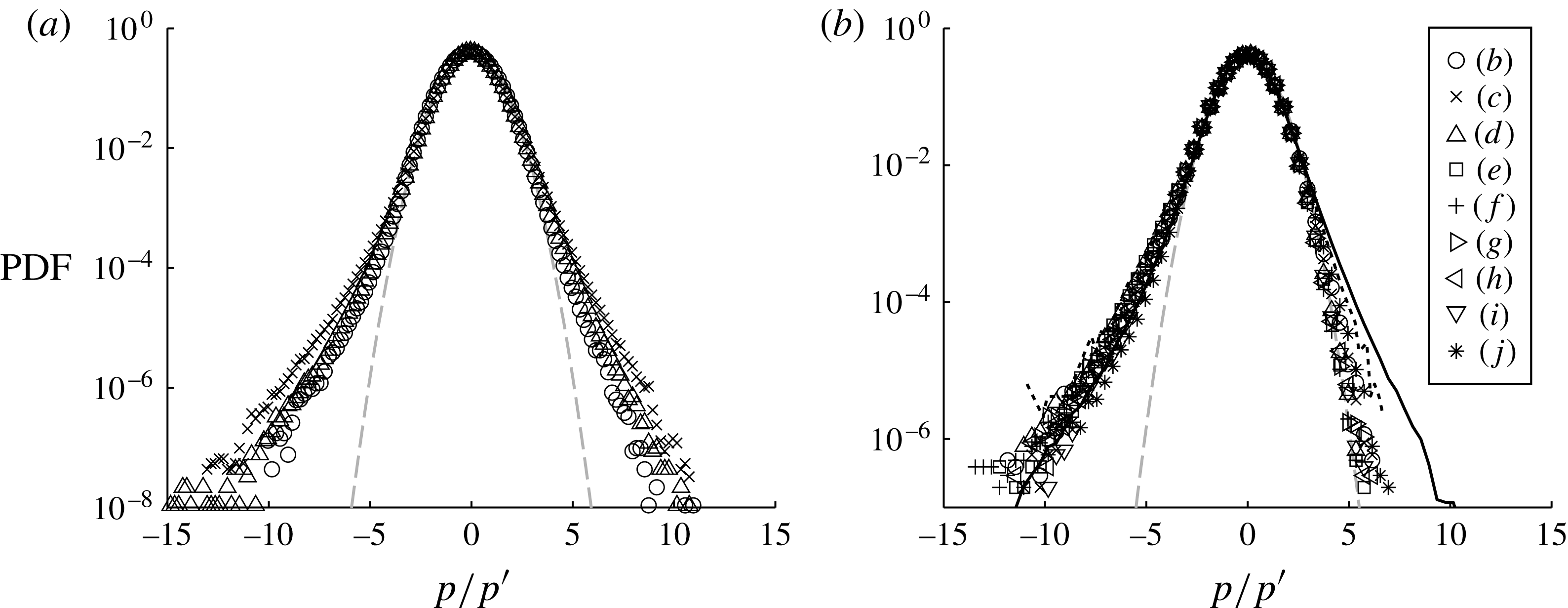
The probability density functions (PDFs) of the pressure fluctuations are shown in figure 11. For the wall pressure, the shape of the PDF does not exhibit clear Reynolds number dependence. The skewness of the wall pressure fluctuations is 0.049, and the flatness is 3.91 at
 $\mathit{Re}_{{\it\theta}}=10\,000$
. These values and the overall shape of the PDF of the present data show a good agreement with those of Tsuji et al. (Reference Tsuji, Fransson, Alfredsson and Johansson2007) and a clear departure from Gaussian behaviour. The slight underestimation of the PDF compared with Tsuji et al. (Reference Tsuji, Fransson, Alfredsson and Johansson2007) could be attributed to the fact that the extra noise existing here attracts the PDF towards the Gaussian curve. For the field pressure fluctuations, the PDF is clearly negatively skewed, and such a feature has been reported in the centre of a jet (Tsuji & Ishihara Reference Tsuji and Ishihara2003) and in the logarithmic region of the turbulent boundary layer (Tsuji et al.
Reference Tsuji, Fransson, Alfredsson and Johansson2007). The skewness and flatness values in the logarithmic region at
 $y_{p}^{+}=237$
, position (e), are
 $-$
0.34 and 3.88 respectively. The relatively large flatness values of the wall and field pressure fluctuations are representative of a strong intermittence of the pressure fluctuation events. In addition, the negatively skewed pressure fluctuations are associated by previous authors (Kim Reference Kim1989; Tsuji et al.
Reference Tsuji, Fransson, Alfredsson and Johansson2007) with vortical motions which create a negative pressure fluctuation inside their core. Close to the edge of the boundary layer, the shape of the PDF is more or less symmetrical, characterized by a skewness of
 $-$
0.069 at position ( j), that is
 $y_{p}/{\it\delta}=1.1$
.
Probability density functions of pressure fluctuations at the wall at three different Reynolds numbers (a) and in the field at the probe positions as in table 5 at
 $\mathit{Re}_{{\it\theta}}=10\,000$
(b). For (a), the symbols are the same as in figure 8. Grey dashed lines, Gaussian;
 $\cdots \cdots$
, Tsuji et al. (Reference Tsuji, Fransson, Alfredsson and Johansson2007) at
 $\mathit{Re}_{{\it\theta}}=10\,500$
and at
 $y^{+}=189$
for the field pressure.
As can be seen, the present experimental data on velocity and pressure fluctuations in a turbulent boundary layer exhibit a good agreement with those previously reported, especially at
 $\mathit{Re}_{{\it\theta}}=10\,000$
. In the next sections, the spatio-temporal pressure–velocity correlations are characterized.
4. Spatio-temporal pressure–velocity correlations
The space–time correlation of the fluctuating pressure and velocity,
 $\boldsymbol{R}_{pu_{i}}$
, is defined here as
 $$\begin{eqnarray}\displaystyle \boldsymbol{R}_{pu_{i}}(y_{p},{\rm\Delta}t,{\rm\Delta}y,{\rm\Delta}z) & = & \displaystyle \overline{p(t+{\rm\Delta}t,y_{p},0)u_{i}(t,y_{p}+{\rm\Delta}y,{\rm\Delta}z)}/{\it\rho}U_{e}^{3}\nonumber\\ \displaystyle & = & \displaystyle \frac{1}{{\it\rho}U_{e}^{3}}\frac{1}{N}\mathop{\sum }_{j=1}^{N}\left\{p(t_{j}+{\rm\Delta}t,y_{p},0)u_{i}(t_{j},y_{p}+{\rm\Delta}y,{\rm\Delta}z)\right\},\end{eqnarray}$$
where
 $t_{j}$
is the time of stereo PIV recording,
 $y_{p}$
is the wall-normal position of the pressure probe,
 ${\rm\Delta}y$
and
 ${\rm\Delta}z$
are the separation of the moving point along
 $y$
and
 $z$
respectively (here
 ${\rm\Delta}z=z$
as
 $z_{p}=0$
),
 ${\rm\Delta}t$
is the time separation of the pressure measurement with respect to
 $t_{j}$
and
 $N$
is the number of samples. These correlations are normalized everywhere by
 ${\it\rho}U_{e}^{3}$
. Since the time-resolved pressure signal is available, the correlation of the velocity field at time
 $t_{j}$
and pressure signal around
 $t_{j}$
is evaluated. It should be noted that, as explained earlier, the wall pressure–velocity correlations are computed from 60 000 and 90 000 independent samples of velocity fields while the field pressure–velocity correlations are evaluated from 10 000 samples.
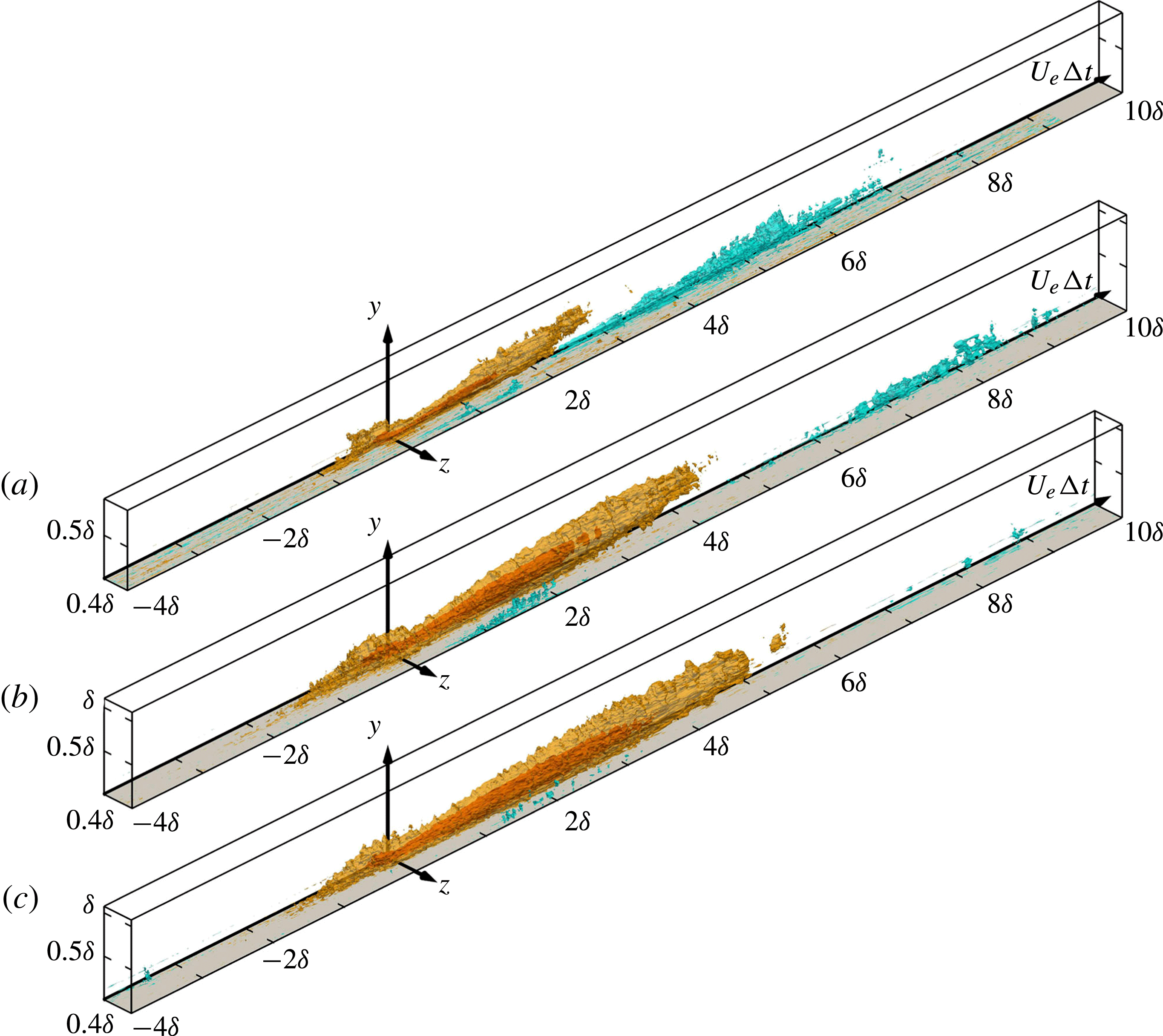
As a first illustration of the results, figure 12 shows a 3D representation of the space–time
 $\boldsymbol{R}_{pu}$
correlation at
 $\mathit{Re}_{{\it\theta}}=10\,000$
at the different pressure reference positions
 $y_{p}$
as given in table 5. Figure 13 gives the same information but at fixed pressure point (b) of table 5 and at three different Reynolds numbers. In these figures, the range of
 ${\rm\Delta}t$
shown is
 $-4\leqslant {\rm\Delta}tU_{e}/{\it\delta}\leqslant 10$
, and the full PIV measurement area is plotted, which is about
 ${\it\delta}\times 0.4{\it\delta}$
in the
 $y$
and
 $z$
directions respectively. As will be seen later, this correlation is the most representative of the elongated large-scale structures of the boundary layer, as it extends to several boundary layer thicknesses. It also has a significant evolution both in
 $y_{p}$
, by a change of shape, and with Reynolds number by a change of size and intensity. Furthermore, a strong difference clearly appears in figure 12 between the correlation with the fixed point at the wall (corresponding to case (a) of table 5) which is quite localized and those in the field (cases (b–j)) which are much more extended in time. Consequently, before looking at what happens in the field, attention will first be focused on case (a) results with the fixed pressure point at the wall, looking at the three
 $\boldsymbol{R}_{pu}$
,
 $\boldsymbol{R}_{pv}$
and
 $\boldsymbol{R}_{pw}$
space–time correlations.
Three-dimensional plots of
 $\boldsymbol{R}_{pu}$
for pressure reference positions (a–j) as in table 5 at
 $\mathit{Re}_{{\it\theta}}=10\,000$
. Contour levels are
 $-2\times 10^{-5}$
(light blue),
 $2\times 10^{-5}$
(orange) and
 $5\times 10^{-5}$
(red).


4.1. Wall pressure–velocity correlations
As was mentioned earlier, with the fixed point at the wall, the correlations converge better when they are averaged on 60 000 (
 $\boldsymbol{R}_{pu}$
) or 90 000 (
 $\boldsymbol{R}_{pv}$
and
 $\boldsymbol{R}_{pw}$
) samples, which is helpful for analysis. Moreover, for interpretation, it is of interest to split the wall pressure fluctuations into two parts: the positive ones which can be associated with a decrease of the wall-parallel (streamwise or spanwise) velocity component (Bernoulli static pressure effect) or an increase of the wall-normal component (stagnation point effect) with respect to the mean. It is in fact just the opposite for negative pressure fluctuations.
Figure 14 gives the
 $\boldsymbol{R}_{pu}$
correlation in the
 ${\rm\Delta}t{-}y$
plane for
 $z/{\it\delta}=0$
for the three Reynolds numbers. In order to estimate the size of the different correlation regions, here and in the following cuts, a thin black contour line is plotted, corresponding to a correlation level of
 $\pm 3\times 10^{-6}$
, which is slightly above the noise level. Thanks to spanwise homogeneity, it is expected that this correlation will be symmetric with respect to the
 $z=0$
plane. As can be observed, it is mostly positive on the negative
 ${\rm\Delta}t$
side and negative on the other side. The time extension and the size along
 $y$
grow significantly with Reynolds number. This is true along
 $z$
as well. The maximum wall-normal extension is of order
 $0.5{\it\delta}$
,
 $0.6{\it\delta}$
and
 $0.8{\it\delta}$
for
 $\mathit{Re}_{{\it\theta}}=7300$
, 10 000 and 18 000 respectively. Taking into account the symmetry with respect to
 $z/{\it\delta}=0$
(due to spanwise homogeneity), the spanwise extent grows up to about
 ${\it\delta}~(\pm {\it\delta}/2)$
at the highest Reynolds number. It is interesting to note that the pressure fluctuations appear located at the leading edge of this large positive ‘structure’. At
 ${\rm\Delta}t=0$
, the maximum of the correlation is slightly above the wall, in the buffer layer. The spanwise extent at
 $\mathit{Re}_{{\it\theta}}=10\,000$
is approximately
 $\pm 0.2{\it\delta}$
at
 ${\rm\Delta}t=0$
, but it increases beyond
 $\pm 0.4{\it\delta}$
when going upstream (negative
 ${\rm\Delta}t$
). The same is true for the wall-normal extension which is maximum at approximately
 ${\rm\Delta}tU_{e}/{\it\delta}\simeq -0.4/-0.6$
. The main effect of the Reynolds number is to increase the size of the positive correlation region in all directions, which means that it does not scale in external variables.
Cuts of the wall pressure
 $\boldsymbol{R}_{pu}$
(case (a) of table 5) in the
 ${\rm\Delta}t{-}y$
plane at
 $z=0$
at
 $\mathit{Re}_{{\it\theta}}=7300$
(a), 10 000 (b) and 18 000 (c).

To refine the analysis, it is of interest to split the correlation between positive and negative pressure fluctuations by conditional averaging. This is done for the intermediate Reynolds number (which is representative of the two others) and plotted in the plane
 $z=0$
in figure 15(a,b) for each sign respectively. In order to get a better view of the 3D structure of these two conditional correlations, two movies are provided as extra electronic supplementary movies available at http://dx.doi.org/10.1017/jfm.2015.158 (movies 1 and 2). The captions of the movies are listed in appendix A.
Cuts of the wall pressure
 $\boldsymbol{R}_{pu}$
(case (a) of table 5) in the
 ${\rm\Delta}t{-}y$
plane at
 $z/{\it\delta}=0$
and at
 $\mathit{Re}_{{\it\theta}}=10\,000$
with (a)
 $p>0$
and (b)
 $p<0$
.

For the positive pressure fluctuations (figure 15
a), two main facts can be noted. (i) The intensity of the positive correlation region, corresponding to positive
 $u$
(i.e. high speed), increases and extends further upstream and downstream down to
 $0.5{\it\delta}/U_{e}$
. A weak elongated negative correlation region appears on the sides of this large upstream positive region extending outside the field of view in span. The spanwise and wall-normal extension of the positive correlation region does not change significantly. (ii) A significant region of negative correlation appears on the positive
 ${\rm\Delta}t$
side, strongly inclined along the wall and attached to it. Plotting it for larger
 ${\rm\Delta}t$
shows that it extends down to about
 $10{\it\delta}/U_{e}$
where it occupies nearly the full boundary layer thickness. It corresponds to negative velocity fluctuations, i.e. to a low-speed region. The only coherent low-speed regions that have been identified previously as extending from the wall up in the boundary layer with such a shape are the hairpin packets of Adrian et al. (Reference Adrian, Meinhart and Tomkins2000), though not on such time extension.
The negative pressure fluctuation correlation is shown in figure 15(b). The shape is completely different. The upstream large positive correlation region disappears completely and is replaced by a very small and intense region very close to the wall and to the fixed point. The dominating feature is a large negative correlation region on the positive
 ${\rm\Delta}t$
side (extending nearly to
 ${\it\delta}$
in
 $y$
,
 $2.5{\it\delta}/U_{e}$
in time and with a spanwise extent of the order of
 ${\it\delta}$
). This region corresponds to high speeds since the pressure fluctuation is negative.
From these figures and movies, it is clear that positive and negative pressure fluctuations at the wall are associated with very different streamwise velocity fluctuation organizations above them. It is thus of interest to look at the correlation with the other fluctuating velocity components, available here thanks to the stereoscopic PIV (SPIV) set-up used.
Figure 16 gives the
 $\boldsymbol{R}_{pv}$
correlation in the
 ${\rm\Delta}t{-}y$
plane for
 $z/{\it\delta}=0$
for the three Reynolds numbers. As can be observed, this correlation is relatively localized in time but, as a difference from
 $\boldsymbol{R}_{pu}$
, it is closer to antisymmetry with respect to the
 ${\rm\Delta}t=0$
axis. The extent is of order 1 in both
 $y/{\it\delta}$
and
 ${\rm\Delta}tU_{e}/{\it\delta}$
, with a maximum of each lobe quite close to the fixed point. It is noticeable that, as a difference from
 $\boldsymbol{R}_{pu}$
, the Reynolds number seems to have little effect on this correlation. In the
 $z=0$
plane of figure 16, both the positive and the negative lobes are at a strong angle to the wall (close to
 $45^{\circ }$
).
Cuts of the wall pressure
 $\boldsymbol{R}_{pv}$
(case (a) of table 5) in the
 ${\rm\Delta}t{-}y$
plane at
 $z=0$
at
 $\mathit{Re}_{{\it\theta}}=7300$
(a), 10 000 (b) and 18 000 (c).

Here again, it is of interest to split the correlation between positive and negative pressure fluctuations by conditional averaging. This is done for the intermediate Reynolds number and is plotted in the
 $z=0$
plane in figure 17(a,b) for each sign respectively. Furthermore, in order to get a better view of the 3D structure of these two conditional correlations, two movies are provided as extra electronic material (movies 3 and 4).
Cuts of the wall pressure
 $\boldsymbol{R}_{pv}$
(case (a) of table 5) in the
 ${\rm\Delta}t{-}y$
plane at
 $z/{\it\delta}=0$
and at
 $\mathit{Re}_{{\it\theta}}=10\,000$
with (a)
 $p>0$
and (b)
 $p<0$
.

The
 $p>0$
correlation of figure 17(a) is dominated by the upstream negative correlation region. The global shape of this correlation is indicative of a strong downward motion upstream of the positive pressure event immediately followed by a weak outward motion downstream, both separated by a sharp interface above the fixed point.
On the contrary, the
 $p<0$
correlation is dominated by the positive correlation region downstream. There is still a significant negative correlation very close to the fixed point and surrounding it. As the pressure fluctuation is now negative, the downstream motion is wallward and the upstream one is outward, just opposite to the previous case, but again with the pressure event just at the interface. As can be seen, the wall-normal velocity fluctuation organization is again significantly different between positive and negative pressure fluctuations at the wall. It should also be noted that the time extension of these correlations is much less than for
 $\boldsymbol{R}_{pu}$
. No near-wall elongated structure is visible.
To complete the picture, it is of interest to look at
 $\boldsymbol{R}_{pw}$
. For homogeneity reasons, this correlation is zero in the
 $z/{\it\delta}=0$
plane and antisymmetric with respect to this plane. Figure 18 gives
 $\boldsymbol{R}_{pw}$
in the
 ${\rm\Delta}t{-}y$
plane for
 $z/{\it\delta}=0.2$
and for the three Reynolds numbers. This correlation is obviously the most complex of the three. Its spanwise extent is larger than the field of view (which is
 $0.4{\it\delta}$
). It is strongly inclined to the wall along
 $z$
(
 $20^{\circ }{-}25^{\circ }$
) and this inclination increases with Reynolds number. It is quite extensive in the wall-normal direction (up to
 $y/{\it\delta}=0.6$
), but also in time, on both positive and negative
 ${\rm\Delta}t$
sides (
 $\pm {\it\delta}/U_{e}$
at the highest Reynolds number). Significant negative correlation regions are observed both downstream of the fixed point (positive
 ${\rm\Delta}t$
) close to the wall and upstream (negative
 ${\rm\Delta}t$
) further away from the wall. Overall, this leads to fairly large
 $w$
motions involved in the wall pressure fluctuations. On increasing the Reynolds number, the positive region strengthens (especially between 7300 and 10 000). The negative downstream region is squeezed against the wall and reduced in intensity. The upstream negative region seems to grow slowly in size and intensity.
Cuts of the wall pressure
 $\boldsymbol{R}_{pw}$
(case (a) of table 5) in the
 ${\rm\Delta}t{-}y$
plane at
 $z/{\it\delta}=0.2$
at
 $\mathit{Re}_{{\it\theta}}=7300$
(a), 10 000 (b) and 18 000 (c).

In figure 19(a,b), the correlation is again split between positive and negative pressure fluctuations, for
 $\mathit{Re}_{{\it\theta}}=10\,000$
and for each sign respectively. In order to get a better view of the 3D structure of these two conditional correlations, two films are provided as extra electronic material (movies 5 and 6).
Cuts of the wall pressure
 $\boldsymbol{R}_{pw}$
(case (a) of table 5) in the
 ${\rm\Delta}t{-}y$
plane at
 $z/{\it\delta}=0.2$
and at
 $\mathit{Re}_{{\it\theta}}=10\,000$
with (a)
 $p>0$
and (b)
 $p<0$
.

For
 $p>0$
, the downstream negative correlation nearly disappears. For
 $p<0$
it is the upstream one that disappears while the downstream one strengthens significantly. The positive region around the fixed point is also quite affected by conditioning. In both cases, the spanwise extension is much wider than the field of view and, as for
 $\boldsymbol{R}_{pv}$
, the time extension of the correlation is limited compared with
 $\boldsymbol{R}_{pu}$
. In fact, these correlations show significant spanwise inward and outward motions at the scale of the boundary layer, coupled in a way that is indicative of large more or less streamwise vortical motions.
Looking at the different plots of the three pressure–velocity space–time correlations presented in figures 14–19 and looking also at movies 1–6, it is clear that the wall pressure is coupled to various coherent flow structures which occupy a large region of the boundary layer. Overall, these pressure fluctuations are sensitive to velocity events inside a box that is about
 ${\it\delta}$
in
 $y$
,
 ${\it\delta}$
in
 $z$
(taking into account the symmetries) and more than
 $[-4{\it\delta}/U_{e},10{\it\delta}/U_{e}]$
in time. These highly correlated velocity events are in fact combinations of the three velocity components which change significantly depending on the pressure fluctuation sign. Figures 20 and 21 try to make a synthesis for each pressure fluctuation sign at
 $\mathit{Re}_{{\it\theta}}=10\,000$
. In each figure, the correlation has been thresholded at a level allowing the main positive and negative regions of each to be highlighted. By looking at movies 1–6, a more complete understanding of the correlation shape is made possible. As it is not easy to understand the full flow structure associated with each pressure event from these separate correlations, two extra movies have been made which combine the three correlations
 $\boldsymbol{R}_{pu},\boldsymbol{R}_{pv}$
and
 $\boldsymbol{R}_{pw}$
in a single 3D representation. The image is presented in the
 $y{-}z$
wall-normal–spanwise plane as a function of time. The
 $\boldsymbol{R}_{pv}$
and
 $\boldsymbol{R}_{pw}$
correlations are represented as vectors in the plane and
 $\boldsymbol{R}_{pu}$
is coded in colour as an out-of-plane component. The two films scan in time through the space–time pressure–‘velocity vector’ correlation. Movies 7 and 8 give the results for positive and negative pressure fluctuations at the wall respectively. Some selected cuts from these two movies are plotted in figures 22 and 23.
Three-dimensional plots of thresholded
 $\boldsymbol{R}_{pu}$
(a),
 $\boldsymbol{R}_{pv}$
(b) and
 $\boldsymbol{R}_{pw}$
(c) correlation for
 $p>0$
at the wall at
 $\mathit{Re}_{{\it\theta}}=10\,000$
. Contour levels are
 $-7.5\times 10^{-6}$
(light blue),
 $1.5\times 10^{-5}$
(orange) for
 $\boldsymbol{R}_{pu}$
,
 $-7.5\times 10^{-6}$
(light blue),
 $6\times 10^{-6}$
(orange) for
 $\boldsymbol{R}_{pv}$
and
 $-7.5\times 10^{-6}$
(light blue),
 $7.5\times 10^{-6}$
(orange) for
 $\boldsymbol{R}_{pw}$
.

Three-dimensional plots of thresholded
 $\boldsymbol{R}_{pu}$
(a),
 $\boldsymbol{R}_{pv}$
(b) and
 $\boldsymbol{R}_{pw}$
(c) correlation for
 $p<0$
at the wall at
 $\mathit{Re}_{{\it\theta}}=10\,000$
. Contour levels are
 $-1.5\times 10^{-5}$
(light blue),
 $9\times 10^{-6}$
(orange) for
 $\boldsymbol{R}_{pu}$
,
 $-7.5\times 10^{-6}$
(light blue),
 $7.5\times 10^{-6}$
(orange) for
 $\boldsymbol{R}_{pv}$
and
 $-7.5\times 10^{-6}$
(light blue),
 $7.5\times 10^{-6}$
(orange) for
 $\boldsymbol{R}_{pw}$
.

Cuts in the
 $y{-}z$
plane of space–time ‘wall pressure’–‘velocity vector’ correlations for
 $p>0$
: (a)
 ${\rm\Delta}tU_{e}/{\it\delta}=-1.46$
; (b)
 ${\rm\Delta}tU_{e}/{\it\delta}=-0.46$
; (c)
 ${\rm\Delta}tU_{e}/{\it\delta}=-0.00$
; (d)
 ${\rm\Delta}tU_{e}/{\it\delta}=0.16$
; (e)
 ${\rm\Delta}tU_{e}/{\it\delta}=0.36$
; (f)
 ${\rm\Delta}tU_{e}/{\it\delta}=0.96$
.

Cuts in the
 $y{-}z$
plane of space–time ‘wall pressure’–‘velocity vector’ correlations for
 $p<0$
: (a)
 ${\rm\Delta}tU_{e}/{\it\delta}=-0.26$
; (b)
 ${\rm\Delta}tU_{e}/{\it\delta}=-0.06$
; (c)
 ${\rm\Delta}tU_{e}/{\it\delta}=0.06$
; (d)
 ${\rm\Delta}tU_{e}/{\it\delta}=0.26$
; (e)
 ${\rm\Delta}tU_{e}/{\it\delta}=0.46$
; (f)
 ${\rm\Delta}tU_{e}/{\it\delta}=0.86$
. The signs of the correlation are flipped to represent the flow pattern associated with the negative wall pressure.

Looking first at the positive pressure fluctuations at the wall, the different correlations plotted in figures 20, 22 and movie 7 give a clear overall picture of a strong sweeping event coming from upstream. Clear traces of streamwise vortices are detectable on both sides, along a line at an angle of
 $\pm 45^{\circ }$
spanwise. This leads to the conclusion that this positive
 $p$
is mostly due to a total pressure effect linked to the
 $v$
component. It is also clear from movie 1 and figure 14 that the large upstream positive correlation region is flanked on both sides by elongated negative correlations close to the wall and extending out of the field of view in span.
For the negative pressure fluctuations at the wall illustrated in figures 21 and 23 and movie 8 (to take into account the fact that
 $p<0$
, the signs of the correlations have been changed to make the movie), low-speed ejection moves down to the wall, pushing the near-wall high streamwise velocity region on the sides and focusing close to the fixed point. It is immediately followed, for
 ${\rm\Delta}t>0$
by a strong sweeping motion focalized at the origin but involving the whole boundary layer thickness. Evidence of streamwise vortices is observable in the nearby low-streamwise-velocity regions. These streamwise vortices, which are relatively large, seem to lift up progressively on increasing
 ${\rm\Delta}t$
.
As can be seen, both positive and negative pressure fluctuations at the wall seem to appear at sharp interfaces of very large organized motions at the scale of the boundary layer thickness. In both cases, the pressure fluctuation seems to be mostly due to strong variations of the wall-normal velocity. It is also important to notice that the large structures appearing upstream for
 $p>0$
and downstream for
 $p<0$
are of the same nature: a strong sweeping motion, involving the whole boundary layer thickness and having a time extension of the order of
 ${\it\delta}/U_{e}$
. These sweeping motions are flanked on both sides by streamwise vortical motions of order
 $0.2{\it\delta}$
in diameter, which are much larger than the usual near-wall streamwise vortices (which are approximately 20 wall units in diameter).
4.2. Field pressure–velocity correlations
Having analysed in detail the pressure–velocity correlations with the fixed pressure point at the wall, it is of interest to look now at what happens in the field since it appeared to be quite different in figure 12.
Looking first at
 $\boldsymbol{R}_{pu}$
, as shown in figure 13, a clear Reynolds number effect is visible on this correlation. It concerns essentially the size, as the overall characteristics of the correlation are similar for the three different Reynolds numbers. To look at the correlation structure, it is interesting to complement figure 12 by cuts in the
 $z=0$
plane, which is a plane of symmetry of this correlation. This is done in figure 24 at
 $\mathit{Re}_{{\it\theta}}=10\,000$
, for positions (b–j) of the pressure point as given in table 5, and in figure 25 for position (b) and for the three Reynolds numbers investigated.
Cuts of the field pressure
 $\boldsymbol{R}_{pu}$
in the
 ${\rm\Delta}t{-}y$
plane at
 $z=0$
and at
 $\mathit{Re}_{{\it\theta}}=10\,000$
. The dotted line indicates the pressure reference position as given in table 5.

Cuts of the field pressure
 $\boldsymbol{R}_{pu}$
correlation in the
 ${\rm\Delta}t{-}y$
plane at
 $z=0$
for three Reynolds numbers (increasing from (a) to (c)) at the reference position (b) in table 5.

At first glance, differently from the pressure point at the wall,
 $\boldsymbol{R}_{pu}$
exhibits an inclined elongated shape on the positive
 ${\rm\Delta}t$
side. At the highest Reynolds number, the near-wall negative lobe extends beyond the limit of the field of view on the positive
 ${\rm\Delta}t$
side (up to
 ${\rm\Delta}tU_{e}/{\it\delta}\sim 18$
at the highest Reynolds number). Both of these positive and negative correlation regions are inclined at a small angle with respect to the
 ${\rm\Delta}t$
axis. This angle decreases when the Reynolds number increases (
 $7^{\circ },5^{\circ }$
and
 $3^{\circ }$
respectively at the three Reynolds numbers for the positive part). Obviously linked to the main elongated positive region, it is present for all Reynolds numbers with comparable size, position and intensity and it extends beyond
 $z/{\it\delta}=0.4$
.
Looking at the main positive correlation region, for wall distances smaller than
 $y_{p}/{\it\delta}\sim 0.15$
(b–f), i.e. in the inner part of the boundary layer, two characteristic patterns are observed: a ‘smaller’ one, which is relatively localized in negative
 ${\rm\Delta}t$
and around the fixed point, and a longer one, which is inclined and elongated in the positive
 ${\rm\Delta}t$
direction with a shallow angle to the horizontal axis. The small region on the negative
 ${\rm\Delta}t$
side is obviously related with the correlation observed for the fixed point at the wall. In this inner region, for a given Reynolds number, the shape and size of the positive correlation region change little with
 $y$
. Beyond
 $y_{p}/{\it\delta}\sim 0.1$
, the two lobes of the positive correlation region merge and form one large correlation pattern. Clearly, the elongated part of the correlation is a wall-attached structure subjected to stretching by convection, which is also supported by the upstream displacement of the structure when moving the fixed point away from the wall. This could be the wall-attached eddies of Townsend.
In order to assess the global shape of this correlation in the inner layer, a movie is provided as extra electronic material for position (b) of table 5 (movie 9). The weak negative correlation on the side of the positive one up to (h), extending significantly outside of the field of view in
 $z$
, is clearly evidenced by this movie, as well as the elongated negative correlation region on the downstream side, extending far outside the field of view, down to
 ${\rm\Delta}tU_{e}/{\it\delta}\sim 18$
.
The second correlation of interest is
 $\boldsymbol{R}_{pv}$
. A cut in the
 ${\rm\Delta}t{-}y$
plane at
 $z=0$
is given in figure 26 at
 $\mathit{Re}_{{\it\theta}}=10\,000$
, which is again highly representative of the shape of this correlation at the three Reynolds numbers. For the purpose of comparison, the correlation with the wall pressure at point (a) is also shown in this figure. As the wall-normal velocity fluctuations are known to be smaller than the streamwise ones the correlation is much weaker than
 $\boldsymbol{R}_{pu}$
(colour scale range is half).
Cuts of the field pressure
 $\boldsymbol{R}_{pv}$
in the
 ${\rm\Delta}t{-}y$
plane at
 $z=0$
and at
 $\mathit{Re}_{{\it\theta}}=10\,000$
. The dotted line indicates the pressure reference position as given in table 5.

From cuts in different planes, it appears that the size and shape of the lobes are very similar in the whole inner region. Taking into account the symmetry with respect to the
 $z=0$
plane, they are approximately
 $0.4{\it\delta}$
in span and
 $0.6{\it\delta}$
in wall-normal extent. In the outer part, the temporal extent of the negative lobe is of the order of
 $4{\it\delta}/U_{e}$
. From plots in the same planes at the two other Reynolds numbers (not shown here), it appears that the effect of this parameter on the size and shape of this correlation is much weaker than for
 $\boldsymbol{R}_{pu}$
.
The last correlation to be analysed is
 $\boldsymbol{R}_{pw}$
. An example is plotted in 3D perspective in figure 27 for pressure reference position (b) at the intermediate Reynolds number
 $\mathit{Re}_{{\it\theta}}=10\,000$
. This is the most complex correlation of the three as it has several distinct regions of each sign and shows significant changes with both wall distance and Reynolds number. Two movies are provided as extra electronic material to show the 3D structure at
 $\mathit{Re}_{{\it\theta}}=10\,000$
in the inner (b) (movie 10) and outer (h) (movie 11) regions respectively. As far as the Reynolds number effect is concerned, it does not greatly change the global picture presented above. The shape of this outer region structure coupling a positive and negative correlation region closely resembles an elongated streamwise oriented vortical structure with a size of the order of the boundary layer thickness. It is interesting to note that, in the pressure creating events, a positive
 $w$
motion in one region is always associated with a negative one above or below it, and vice versa, which is indicative of streamwise vortical motions.
Three-dimensional representation of
 $\boldsymbol{R}_{pw}$
at
 $\mathit{Re}_{{\it\theta}}=10\,000$
for pressure reference position (b) as given in table 5. Contour levels are
 $-8\times 10^{-6}$
(light blue),
 $8\times 10^{-6}$
(orange) and
 $1.6\times 10^{-5}$
(red).

To complete this analysis and in the context of the ongoing research around large-scale structures in turbulent boundary layers, it is of interest to emphasize some specific Reynolds number effects. The extension and location of
 $\boldsymbol{R}_{pu}$
changes significantly in the wall-normal direction, while the spanwise extension is nearly the same. This wallward extension is accompanied by a downward motion of
 $\boldsymbol{R}_{pw}$
.
This strong Reynolds number influence is visible in figure 28, which shows
 $\boldsymbol{R}_{pu}$
in the
 $z=0$
plane at point (i) corresponding to
 $y_{p}/{\it\delta}\simeq 0.8$
at the three Reynolds numbers.
Cuts of the field pressure
 $\boldsymbol{R}_{pu}$
correlation in the
 ${\rm\Delta}t{-}y$
plane at
 $z=0$
, at the pressure reference position (i) in table 5 and for different Reynolds numbers (increasing from (a) to (c)).

As for the wall pressure correlations, in order to assess the global flow structure associated with the correlation shapes, it is of interest to make movies combining the three correlations in a single representation. The correlation has been here again conditioned on the sign of the local fluctuating pressure. What happens close to the wall in the inner layer is focused on. Point (c) located at
 $y^{+}=56$
, i.e. in the buffer layer, is selected for this. Movie 12 corresponds to
 $p>0$
and movie 13 to
 $p<0$
. Specific cuts in the
 $y$
–
 $z$
plane are given at different
 ${\rm\Delta}t$
in figures 29 and 30.
Cuts in the
 $y{-}z$
plane of space–time ‘field pressure’–‘velocity vector’ correlations for
 $p>0$
: (a)
 ${\rm\Delta}tU_{e}/{\it\delta}=0.00$
; (b)
 ${\rm\Delta}tU_{e}/{\it\delta}=0.35$
; (c)
 ${\rm\Delta}tU_{e}/{\it\delta}=0.99$
; (d)
 ${\rm\Delta}tU_{e}/{\it\delta}=3.70$
; (e)
 ${\rm\Delta}tU_{e}/{\it\delta}=6.02$
; (f)
 ${\rm\Delta}tU_{e}/{\it\delta}=8.01$
. The probe position is position (c) in table 5.

Cuts in the
 $y{-}z$
plane of space–time ‘field pressure’–‘velocity vector’ correlations for
 $p<0$
: (a)
 ${\rm\Delta}tU_{e}/{\it\delta}=-0.57$
; (b)
 ${\rm\Delta}tU_{e}/{\it\delta}=-0.07$
; (c)
 ${\rm\Delta}tU_{e}/{\it\delta}=0.07$
; (d)
 ${\rm\Delta}tU_{e}/{\it\delta}=0.86$
; (e)
 ${\rm\Delta}tU_{e}/{\it\delta}=3.03$
; (f)
 ${\rm\Delta}tU_{e}/{\it\delta}=5.04$
. The probe position is position (c) in table 5. The signs of the correlation are flipped to represent the flow pattern associated with the negative wall pressure.

Looking first at positive pressure fluctuations (movie 12 and figure 29), the flow structure observed for negative
 ${\rm\Delta}t$
is completely similar to the one appearing in movie 7 and figure 22 for positive wall pressure fluctuations. This explains why no cuts are provided in figure 29 which focuses on the positive
 ${\rm\Delta}t$
part. In this region, the flow structure observed is very different from that obtained with the wall pressure probe. At
 ${\rm\Delta}tU_{e}/{\it\delta}=0.35$
, although an outward motion is visible in the outer part, a strong high-streamwise-velocity region is still present in the inner layer with clear traces of streamwise vortices and downward motion due to them. This high-speed region extends progressively outward, flanked by the vortices which move progressively outwards too. At
 ${\rm\Delta}tU_{e}/{\it\delta}=3.7$
, the high-speed region influences the whole boundary layer thickness, the vortices are localized around
 $0.35{\it\delta}$
and a global sweeping motion is induced between them. A low-speed region starts to appear at the wall. Downstream, the high-speed region fades away while the low-speed region develops and occupies approximately
 ${\it\delta}/2$
at
 ${\rm\Delta}tU_{e}/{\it\delta}=8$
. Some vortical motions and weak ejections are detectable inside this low-speed region but these are much less coherent than those associated with the preceding high-speed region. It should be remembered that the symmetry of the correlations is enforced here by the spanwise homogeneity, which means that the counter-rotating vortex pairs observed are statistical and can be the result of many single vortices of the same sign. It is clear nevertheless that a streamwise vortex on the side of a high-speed region is rotating in order to contribute to downward motion of the fluid. What is also obvious is that on average, these streamwise vortical motions have a size of the order of
 $0.1{\it\delta}$
, which is much larger than the wall generated vortices found in this type of flow (Tanahashi et al.
Reference Tanahashi, Kang, Miyamoto, Shiokawa and Miyauchi2004; Herpin et al.
Reference Herpin, Stanislas, Foucaut and Coudert2013). Finally, it seems that the flow structure sensed by the field pressure on the positive
 ${\rm\Delta}t$
is not directly related to the one at the wall which, looking at movie 7 and figure 22, shows a very quick fading of the high-speed region after
 ${\rm\Delta}t=0$
and the development of a low-speed near-wall region at
 ${\rm\Delta}tU_{e}/{\it\delta}=0.35$
.
The negative pressure fluctuation case is described by movie 13 and figure 30. Here, the near-wall region is dominated by a low-speed elongated structure which appears at approximately
 ${\rm\Delta}tU_{e}/{\it\delta}=-0.6$
and disappears at approximately
 ${\rm\Delta}tU_{e}/{\it\delta}=5$
. This low-speed region, which is originally of weak ejection type, is perturbed just after
 ${\rm\Delta}t=0$
by a strong and focalized sweeping motion which is sensed also by the wall pressure (compare figures 23 and 30 at
 ${\rm\Delta}tU_{e}/{\it\delta}=0.06$
). However, as a difference here, the low-speed region is not suppressed, it redevelops under the high-speed sweep which moves away from the wall and evidences a strong ejection fed by strong near-wall vortical structures at the scale of the inner layer (
 $0.1{-}0.2{\it\delta}$
). Both the low-speed region and the vortical structures stay attached to the wall down to approximately
 ${\rm\Delta}tU_{e}/{\it\delta}=1.5$
. The outer high-speed sweeping region disappears around this time, allowing both the low-speed region and the companion vortices to lift progressively away from the wall and to disappear at approximately
 ${\rm\Delta}tU_{e}/{\it\delta}=5$
. A near-wall high-speed region develops from
 ${\rm\Delta}tU_{e}/{\it\delta}=4$
, but with no clear evidence of vortices or ejection.
As can be seen, apart from the strong sweep after
 ${\rm\Delta}t=0$
, this second case is quite different from what is correlated with the wall pressure.
5. Discussion
Having analysed in some detail the results obtained in the present experiment, it is of interest to compare them with the existing knowledge and to put them alongside other data so as to achieve clearer insight into the physics of pressure–velocity interaction in the turbulent boundary layer.
Looking at the pressure–velocity correlations, those with the pressure point at the wall have their maximum relatively close to the wall. It is then of interest to compare them with DNS data which are free from acoustic noise. This is done in figures 31 and 32 with the channel flow DNS of Del Álamo et al. (Reference Del Álamo, Jiménez, Zandonade and Moser2004) which allow a good statistical convergence. Figure 31 gives the
 $\boldsymbol{R}_{pu}$
and
 $\boldsymbol{R}_{pv}$
correlations with the fixed pressure point at the wall in a streamwise wall-normal
 $x{-}y$
plane for the DNS and the
 ${\rm\Delta}t$
–
 $y$
plane for the boundary layer. Coordinates are scaled in wall units while the amplitude of the correlation is scaled with
 $u_{{\it\tau}}$
. The same information is given for
 $\boldsymbol{R}_{pu}$
and
 $\boldsymbol{R}_{pw}$
in the
 $y{-}z$
plane in figure 32. Although they are obtained at different Reynolds numbers (
 $\mathit{Re}_{{\it\tau}}=950$
for the channel flow and 3509 for the boundary layer), the agreement is relatively good on both the shape and the size of these correlations in the two planes with this wall scaling. The main difference is in the
 $\boldsymbol{R}_{pu}$
correlation in the streamwise plane which keeps the same shape but shows a wider extension in both directions (it should be remembered that space and time are compared on the horizontal axis here). As far as the amplitude of the correlations is concerned, the experimental data are slightly lower than the DNS ones. As suggested by Tsuji et al. (Reference Tsuji, Imayama, Schlatter, Alfredsson, Johansson, Marusic, Hutchins and Monty2012), this could be attributed to a spatial averaging effect of the pressure probe leading to an attenuation of the pressure signal compared with the DNS. Correlations conditioned with the sign of the wall pressure fluctuation show a striking similarity.
The
 $\boldsymbol{R}_{pu}$
and
 $\boldsymbol{R}_{pv}$
wall pressure–velocity correlations in the
 $x{-}y$
plane of a plane channel flow at
 $\mathit{Re}_{{\it\tau}}=950$
(a,b) (Del Álamo et al.
Reference Del Álamo, Jiménez, Zandonade and Moser2004) and in the
 ${\rm\Delta}t$
–
 $y$
plane of the flat plate boundary layer at
 $\mathit{Re}_{{\it\tau}}=3509$
(c,d).

The
 $\boldsymbol{R}_{pu}$
and
 $\boldsymbol{R}_{pw}$
wall pressure–velocity correlations in the
 $y{-}z$
plane for a plane channel flow at
 $\mathit{Re}_{{\it\tau}}=950$
(a,b) (Del Álamo et al.
Reference Del Álamo, Jiménez, Zandonade and Moser2004) and for the flat plate boundary layer at
 $\mathit{Re}_{{\it\tau}}=3509$
(c,d).

These comparisons are interesting from two points of view. First, they show that the wall pressure, although correlated with a large part of the boundary layer velocity field, does not depend strongly on the outer part, which is quite different between a plane channel and a boundary layer. As shown by Mathis, Hutchins & Marusic (Reference Mathis, Hutchins and Marusic2009), it is dependent on the logarithmic layer, which is confirmed here by the size of the significant correlation region. Second, although the Taylor hypothesis is highly questionable in such a shear flow and on such time scales, it appears that the spatial correlations in the channel and the spatio-temporal ones in the boundary layer show very similar shapes and sizes in wall unit scaling, despite the difference in Reynolds number.
Looking now at other experimental contributions, the most detailed one on the relation between wall pressure fluctuations and the flow coherent motions is by Thomas & Bull (Reference Thomas and Bull1983). These data were not obtained by correlation as carried out here, but by conditional sampling, and only the streamwise velocity component was measured using a single hot-wire positioned at different wall distances. Moreover, both the wall pressure and the wall shear stress were measured simultaneously. Figure 1(d), taken from this study, has a striking similarity with the shape of the
 $\boldsymbol{R}_{pu}$
correlation observed here for positive wall pressure fluctuations (see for example movie 1 and figure 15
a). Figure 1(b) shows a sketch by these authors of the trace of the wall pressure conditioned on large pressure events (a real trace is plotted in their figure 5).
Time trace of the wall pressure. The same detection method as in Thomas & Bull (Reference Thomas and Bull1983) using the smoothed rectified high-frequency component of the wall pressure is employed to perform ensemble averaging. The resulting pressure signal is scaled by the ratio of friction velocities and compared with the one of Thomas & Bull (Reference Thomas and Bull1983). The grey line indicates the result of Thomas & Bull (Reference Thomas and Bull1983) and the black line shows the present data.

Comparison between Thomas & Bull (Reference Thomas and Bull1983) and the present experiments.

For the purpose of comparison, the same processing method, with the same cutoff frequency of the low-pass filter (
 ${\it\omega}_{c}{\it\delta}^{\ast }/U_{e}=0.43$
), was applied to the present pressure signal. The result is compared with Thomas & Bull (Reference Thomas and Bull1983) in figure 33, where the conditioned pressure signal is scaled with the r.m.s. of the original signal. It is of interest at this stage to compare the two experimental conditions. This is done in table 6. As can be seen, the Reynolds number is nearly the same, but obtained with very different velocities and boundary layer thicknesses. There is a ratio of nearly 7 between the free-stream velocities, the boundary layer thicknesses and the friction velocities. As can be seen from figure 33, the present signal is similar to the one in Thomas & Bull (Reference Thomas and Bull1983) but much smaller in amplitude (the present data are multiplied here arbitrarily by 10 for the purpose of comparison in the figure). The agreement on the overall shape appears to be relatively satisfactory between the two signals, but there is an obvious scaling problem in both amplitude and time. The scaling of the wall pressure fluctuations was addressed in § 3 and figure 9. As mentioned by Bull (Reference Bull1996), the different parts of the wall pressure spectrum scale differently. As the low-frequency range, which scales with
 ${\it\delta}^{\ast }$
and
 $U_{e}$
, corresponds to times
 $T$
so that
 $TU_{e}/{\it\delta}^{\ast }>200$
(Farabee & Casarella Reference Farabee and Casarella1991; Bull Reference Bull1996), the present conditionally averaged signals appear to correspond more to the mid-frequency range part of the spectrum for which the scaling is still not clear between
 $U_{e}$
and
 ${\it\tau}_{w}$
. It seems acceptable from figure 9 that the r.m.s. of the pressure fluctuations at the wall scales in wall units with a weak Reynolds number dependence. Figure 33 seems to indicate that the large-scale fluctuations (as conditioned by Thomas & Bull Reference Thomas and Bull1983) do not scale with the r.m.s. value, either in amplitude where a ratio of about 10 is evidenced between the two experiments at nearly the same Reynolds number, or in time as a factor of order 2 is observed on
 ${\rm\Delta}tU_{e}/{\it\delta}^{\ast }$
.
The difference in convergence can be explained by the number of samples, which was
 $4\times 10^{4}$
in the experiment of Thomas & Bull (Reference Thomas and Bull1983) and is
 $10^{8}$
in the present case. Part of the difference in amplitude can be explained by the low-pass filtering effect. Since the time scale ratio between the two experiments is of the order of 50, the valid frequency range of Thomas & Bull (Reference Thomas and Bull1983), which is given as 200 Hz–6.25 kHz, corresponds to 4–127 Hz in the present experiment, compared with 1 Hz–1 kHz in the present case. Moreover, their sampling rate of 12.5 kHz corresponds to 254 Hz in the present measurements, compared with 40 kHz. These differences may explain part of the differences observed. Unfortunately, there is no indication in the paper of Thomas & Bull (Reference Thomas and Bull1983) on the r.m.s. level of pressure fluctuations and on their scaling with
 ${\it\tau}_{w}$
.
Besides these differences, the global behaviour of the signal is convincingly similar. In fact, in the light of the difference observed here between the correlation conditioned by positive and negative pressure fluctuations, the smoothed rectified signal used by Thomas & Bull (Reference Thomas and Bull1983) appears to be questionable. Based on the present results, their conditional approach seems to be dominated by the positive pressure fluctuations at the wall. The same sign separation should be performed in the conditioning procedure, as was done by Johansson et al. (Reference Johansson, Her and Haritonidis1987) and Naguib, Wark & Juckenhöfel (Reference Naguib, Wark and Juckenhöfel2001). Moreover, looking at figure 33, the characteristic time of the conditional signal is of the order of
 $20{\it\delta}^{\ast }/U_{e}$
while the cutoff of the low-pass filter was set by Thomas & Bull (Reference Thomas and Bull1983) at
 $15{\it\delta}^{\ast }/U_{e}~({\it\omega}_{c}{\it\delta}^{\ast }/U_{e}=0.43)$
. Based on figures 33 and 1(b), a cutoff frequency corresponding to
 $5{\it\delta}^{\ast }/U_{e}$
seems more appropriate.
Nevertheless, two important facts can be observed in figure 33: the strong positive pressure fluctuation is followed by a negative fluctuations of the same order, which is confirmed by the present results. This could be linked with the rapid change of the large-scale pressure–velocity correlations (especially
 $\boldsymbol{R}_{pv}$
) which occurs close to
 ${\rm\Delta}t=0$
in the present results, especially if the conditioned signal is dominated by positive wall pressure fluctuations, as hypothesized above.
As shown by Thomas & Bull (Reference Thomas and Bull1983), small-scale pressure fluctuations, obviously linked to small-scale wall shear stress fluctuations, override the raising front of the large-scale one (figure 1 c). These intense small-scale pressure fluctuations are linked to near-wall energetic small scales which are not resolved by the present PIV set-up.
The comparison with the abovementioned contribution of Johansson et al. (Reference Johansson, Her and Haritonidis1987) and Naguib et al. (Reference Naguib, Wark and Juckenhöfel2001) is more difficult. As the Reynolds number is much lower, they focused more on the near-wall region which is not well resolved here and they used hot-wire time-resolved velocity data which are not available in the present study. Nevertheless, it is of interest to compare the wall pressure signature as they used a condition on the high-pressure peaks different from Thomas & Bull (Reference Thomas and Bull1983). The same condition (
 $|p_{w}^{\prime }|>k\cdot p_{rms}^{\prime }$
) was applied on the present wall pressure at
 $\mathit{Re}_{{\it\theta}}=10\,000$
and the result is plotted in figure 34 with the same scaling for both positive and negative high-pressure peaks. The same value of
 $k=2.5$
was used as these authors used for their analysis. The agreement with Johansson et al. (Reference Johansson, Her and Haritonidis1987) is convincing. As far as the flow structure is concerned, these authors use only strong pressure peaks of one sign to conditionally average the velocity while here, all pressure fluctuations of the same sign are correlated with the velocity. Nevertheless, figure 15(a) is in good agreement with the results of Naguib et al. (Reference Naguib, Wark and Juckenhöfel2001) at
 $y^{+}=200$
. Figure 15(b) is also in good agreement with the fact that a negative pressure peak is coupled with a sweeping type of motion.
Ensemble averaged wall pressure fluctuation conditioned by the high-pressure peak event. Here,
 $k$
is the threshold for the high-pressure events.

The new element in the present results is the fact that the negative wall pressure fluctuations correlate with a flow structure that is very different from that evidenced by Thomas & Bull (Reference Thomas and Bull1983). This is probably explained by the conditional averaging procedure used by these authors which is quite different from the present correlation approach. In the present results, in both cases, a large part of the outer boundary layer is involved in a large bulge of high speeds, upstream of the fixed point for
 $p>0$
and downstream for
 $p<0$
. A very elongated coherent near-wall region can also be identified in both cases. It is low speed and downstream for
 $p>0$
and high speed upstream and downstream for
 $p<0$
. In the case of positive
 $p$
, the negative correlation region associated with this near-wall low-speed region can be tracked down to
 ${\rm\Delta}tU_{e}/{\it\delta}=7{-}8$
. This structure is not a classical near-wall streak, as it extends up to
 $y/{\it\delta}=0.18~(y^{+}=650)$
at
 ${\rm\Delta}tU_{e}/{\it\delta}=3$
, which is much further away from the wall. This means that even above the viscous and buffer layers, some coherent motions which originate at the wall and seem somehow decoupled from the outer part of the boundary layer have a very long lifetime.
Looking now at the field pressure–velocity correlation, the main result obtained here is that on top of the correlation structure observed with the wall pressure, a new coherent region is observed in the correlation, which appears to be relatively independent of the first one. This coherent region is highly elongated in time for both
 $u$
and
 $w$
while it appears more localized for
 $v$
. These results cannot be compared with previous experimental ones as none could be found by the authors. They can nevertheless be compared with other correlations obtained previously in other experiments performed in the same facility. This is done in figure 35, which compares cuts of the
 $\boldsymbol{R}_{pu}$
correlation in the
 $z=0$
plane (like those already shown in figure 24 for
 $\mathit{Re}_{{\it\theta}}=10\,000$
) with the streamwise velocity correlation
 $\boldsymbol{R}_{uu}$
at comparable wall distances obtained with a rake of hot-wires by Tutkun et al. (Reference Tutkun, George, Delville, Stanislas, Johansson, Foucaut and Coudert2009). The comparison is made at the highest Reynolds number (
 $\mathit{Re}_{{\it\theta}}=18\,000$
), for three positions of the fixed point (namely
 $y^{+}=105$
, 445 and 1805) corresponding to cases (c), (e) and (g) of table 5 at
 $y^{+}=101$
, 424 and 1715. The same overall shape, strongly elongated and inclined downstream, can be observed on the two types of correlations. Two significant differences are evidenced. The position of the fixed point with respect to the correlation pattern is more central for the
 $\boldsymbol{R}_{uu}$
correlation than for the
 $\boldsymbol{R}_{pu}$
one. The second difference is in the size of this positively correlated elongated region. It is relatively invariant with
 $y$
for
 $\boldsymbol{R}_{pu}$
(but shifting upstream), while it is obviously growing with wall distance for
 $\boldsymbol{R}_{uu}$
(while keeping its position with respect to the fixed point). The size of the
 $\boldsymbol{R}_{pu}$
positive region appears to be comparable to the size of
 $\boldsymbol{R}_{uu}$
at the largest wall distance (
 $y^{+}=1805$
).
Cuts of
 $\boldsymbol{R}_{pu}$
in the
 ${\rm\Delta}t{-}y$
plane at
 $z=0$
and at
 $\mathit{Re}_{{\it\theta}}=18\,000$
compared with the
 $\boldsymbol{R}_{uu}$
space–time correlation from Tutkun et al. (Reference Tutkun, George, Delville, Stanislas, Johansson, Foucaut and Coudert2009) at the same Reynolds number and at wall distances corresponding to cases (c), (e) and (g) in table 5.

Very recently, an original study, complementary to the present one, has been published by Ghaemi & Scarano (Reference Ghaemi and Scarano2013). They use a completely different approach to assess the relation between the high-amplitude pressure peaks (HAPPs) and the velocity field in the near-wall region of a turbulent boundary layer. A time-resolved tomo-PIV experiment is performed from which the instantaneous 3D pressure field can be recovered together with the three-dimensional, three-components and time-resolved velocity and acceleration fields. Due to the limitations of time-resolved tomo-PIV, the Reynolds number of the experiment is
 $\mathit{Re}_{{\it\theta}}=1900$
and the field of view is limited to
 $418\times 149\times 621$
wall units along
 $x$
,
 $y$
and
 $z$
respectively. Although the difference in Reynolds number is up to one order of magnitude, and the field of view is much wider here, it is of interest to compare the results obtained. The analysis of Ghaemi & Scarano (Reference Ghaemi and Scarano2013) is focused on high-pressure peaks (both positive and negative) in the near-wall region and on the flow organization associated with them. It is based on the analysis of individual realizations and on conditional averaging. As results are available only in the near-wall region (
 $y^{+}<113$
), comparison makes sense only in relation to the wall pressure correlations obtained here. Looking first at the positive pressure fluctuations, their conditional velocity field surrounding a positive HAPP has a striking similarity with the present result for the wall pressure–velocity correlation, as illustrated by movie 10. The same sweep upstream/ejection downstream with the same
 $y{-}z$
plane flow pattern on both sides of the fixed point is observed in both cases. The main difference is in the scale of the event, which is of the order of
 ${\it\delta}$
in the present case while it is much more localized near the wall in the other study. In fact, in that study, the ejection occurring just downstream of the fixed point is clearly associated with a hairpin type of vortical structure located just downstream of it and ‘surrounding’ it with its legs. It is clear that the present data do not resolve these near-wall structures which appear in Ghaemi & Scarano (Reference Ghaemi and Scarano2013) below
 $y^{+}<50$
. Nevertheless, their results indicate some evidence of hairpin packets. A possible explanation is that the correlation observed here on the positive
 ${\rm\Delta}t$
side is the signature of a hairpin packet originating at the fixed point and from which Ghaemi & Scarano (Reference Ghaemi and Scarano2013) see only the very first (and partially the second one). Such hairpin packets should imprint a correlation of the ejection side very similar to what a single vortex is doing near the fixed point, and this is the case. The only problem is that the individual vortices are smeared out by the correlation averaging procedure, because of their possible variability in number, size, intensity and position.
Looking now at the negative pressure fluctuations, a comparison between the results of Ghaemi & Scarano (Reference Ghaemi and Scarano2013) and the present movie 11 shows a striking overall similarity: strong and short ejection upstream with low streamwise velocity above the axis surrounded by high streamwise velocity on the sides and then a sweeping motion coming from above down to the wall shortly after the fixed point. The main difference here again is in the scale of the event, which here involves most of the boundary layer, while in the quoted study structures are much more localized near the wall. Moreover, the streamwise vortices evidenced by these authors upstream in the
 $y{-}z$
plane are not detectable in the present results, which clearly show large vortices inclined with respect to the wall on both sides of the downstream sweeping motion. It should be mentioned that Ghaemi & Scarano (Reference Ghaemi and Scarano2013) come to the conclusion that, in the near-wall region, negative HAPPs are mostly associated with vortex cores, of both hairpin and streamwise type. The present data cannot resolve those hairpins which are of the order of 50 wall units. They seem to indicate that these near-wall vortex cores which generate strong negative pressure peaks are here preferably associated with a large flow structure which has strong similarity with the near-wall local one.
Coming back to the movies plotting the three correlations together (movies 7, 8, 12 and 13), they give a clear and detailed insight into the relation between the pressure and the flow structure. The field pressure/velocity conditional correlation at point (c), which is well in the inner layer (
 $y^{+}=56$
,
 $y/{\it\delta}=0.016$
), appears to be sensitive to the same structures as those evidenced by the wall pressure correlations (especially for
 $p>0$
). Moreover, it clearly shows a distinctive flow structure with a very long lifetime. At this stage, it is important to recall that the correlation is a statistical operator which averages all the flow events wherever and whenever they occur. Thanks to the spanwise homogeneity of the flow, statistically, all possible events can happen at each point in the span if the sampling duration is long enough. This means that the characteristic flow structures that are observed in the correlations and which differ between the wall and field pressure sets can be disconnected in space and time. This probably explains why the elongated structures sensed by the field pressure probe are not visible in the wall pressure data.
The second important aspect to note is that, in the field, a positive pressure fluctuation is associated with a high streamwise velocity motion, while a negative pressure fluctuation is associated with a low-speed one. Intuitively, the opposite would be expected: high pressure/low streamwise velocity and low pressure/high streamwise velocity. This means that the streamwise velocity component, although dominant in this region (to give orders of magnitude, at this probe position, the mean streamwise velocity is of order
 $U_{e}/10$
,
 $u^{\prime }$
is comparable to this local mean and
 $v^{\prime }$
is
 $0.4u^{\prime }$
), is not the one driving the pressure fluctuations. This is clear at the wall where, from the present results, the wall pressure sign appears to be driven by the wall-normal motions. This was not so evident, a priori, in the field. Looking at movies 12 and 13, the strong vortical structures evidenced on the sides of the elongated streamwise velocity structures induce significant wall-normal components at the position of the probe, which probably explains the result found here.
The next important fact to notice is that the field pressure correlations enable two types of elongated structures to be observed. These are high-speed sweeps and low-speed ejections which have a very significant time extension and spatial size. These structures seem to travel in the flow accompanied by streamwise vortical structures on their side and without influencing the wall pressure significantly. The large structure influencing the wall pressure most appears to be of sweeping type but more compact in time, so that it looks like a local event with a sweep/ejection sequence for
 $p>0$
and an ejection/sweep for
 $p<0$
following each other in a very short time.
Sketch of near-wall turbulence organization from Blackwelder & Kaplan (Reference Blackwelder and Kaplan1976).

Looking at the elongated structures shown by the field pressure correlation, it is striking that the picture obtained looks very similar to the one proposed many years ago for the near-wall streaks, as illustrated by figure 36 from Blackwelder & Kaplan (Reference Blackwelder and Kaplan1976). The picture is the same, but the scale is completely different. The vortical structures have a size comparable to the inner layer (
 $0.1{-}0.2{\it\delta}$
), and the low-speed and high-speed ‘streaks’ are of order
 ${\it\delta}$
in
 $y$
and
 $z$
and a time extension difficult to estimate as it is very long (
 $10{\it\delta}/U_{e}$
at least). This is in very good agreement with the very-large-scale motions (VLSMs) found by Tomkins & Adrian (Reference Tomkins and Adrian2003), Ganapathisubramani, Clemens & Dolling (Reference Ganapathisubramani, Clemens and Dolling2006) and Hutchins & Marusic (Reference Hutchins and Marusic2007) in various high-Reynolds-number boundary layers. The low-speed structure evidenced by the
 $p>0$
correlation can be associated with the hairpin packets of Adrian et al. (Reference Adrian, Meinhart and Tomkins2000), if the vortical structures observed here on the sides of these low-speed regions are thought of as averages of different hairpins fluctuating in space and time. (The same type of effect is obtained, for example, with a long time averaging of a tip vortex which has an unsteady position. The result is a larger and smoother vortex.) This implies that the vortex packets follow each other in trains. The high-speed one, linked to
 $p<0$
, has, for the moment, not been evidenced at this scale, but can be easily understood. Looking carefully at movies 12 and 13, clear evidence of structures of the opposite sign and comparable size is visible on the spanwise side of the main structure developing in the middle of the field of view, and this is the case for both
 $p>0$
and
 $p<0$
. Once more, this spanwise staggering is in good agreement with the observations of Tomkins & Adrian (Reference Tomkins and Adrian2003), Ganapathisubramani et al. (Reference Ganapathisubramani, Clemens and Dolling2006) and Hutchins & Marusic (Reference Hutchins and Marusic2007), and the whole picture provided by the present correlations is supported by the fact found by these authors that the long streaks move slowly in span (see figure 4 of Hutchins & Marusic Reference Hutchins and Marusic2007 and figure 2 of Ganapathisubramani et al.
Reference Ganapathisubramani, Clemens and Dolling2006). It is also in good agreement with the results of Kobashi & Ichijo (Reference Kobashi and Ichijo1986) for the structures influencing the wall pressure. To push further the comparison with the near-wall region, it was shown by Stanislas et al. (Reference Stanislas, Perret and Foucaut2008) and Herpin et al. (Reference Herpin, Stanislas, Foucaut and Coudert2013) that the vortices generated by the instability of the near-wall streaks have a radius that is universal in Kolmogorov scaling and which is of the order of
 $8{\it\eta}$
. Close to the wall, the Kolmogorov scale is relatively constant and close to 2 wall units. This means that the radius of the streamwise vortices is close to 16 wall units and that the peak of the turbulent kinetic energy is then close to the centre of the near-wall streamwise vortices. Looking at figure 8, the plateau in
 $u^{\prime }$
, which is known from Marusic & Kunkel (Reference Marusic and Kunkel2003) and Hultmark et al. (Reference Hultmark, Vallikivi, Bailey and Smits2013) to develop into a second peak on increasing the Reynolds number, starts at approximately
 $y^{+}\simeq 100$
. It is not so pronounced at
 $\mathit{Re}_{{\it\theta}}=10\,000$
, but clearly visible at
 $\mathit{Re}_{{\it\theta}}=18\,000$
. Looking at the streamwise vortical structures evidenced at
 $\mathit{Re}_{{\it\theta}}=10\,000$
in movies 12 and 13 and in figures 29 and 30, their centres appear initially at
 $y/{\it\delta}\simeq 0.05$
and move slowly away up to
 $0.3{-}0.4{\it\delta}$
; that is, at this Reynolds number, from
 $y^{+}\simeq 150$
to approximately 1000. By analogy, this second peak could be associated with these streamwise vortical structures. The fact that these vortical structures are much more elongated than the near-wall ones and that they move relatively far away from the wall should explain the fact that this second peak looks more like a plateau compared with the first one.
Therefore, the idea is that the large streamwise vortical motions are mainly responsible for this second turbulence peak but also for the sweeping/ejection motion in the alternating streamwise elongated respectively high- and low-speed bulges. The smoothing properties of the correlation operator give a simplified picture with enforced symmetry. The instantaneous pictures provided by recent high-Reynolds-number DNS of channel flow (Jiménez Reference Jiménez2013) show that this is an average view which is difficult to recognize in instantaneous realizations. Nevertheless, from the modelling point of view, this provides a significant reduction in complexity as the full high-Reynolds-number boundary layer process can be simplified into two relatively similar streaky structure systems including the same ingredients: low- and high-speed streaks, ejections and sweeps and streamwise vortices between the streaks, rotating so as to lift the low-speed regions and to sweep down the high-speed ones. The first system is inner, at the scale of the buffer layer (scaling in wall units), and the other outer, at the scale of the boundary layer itself. Both of these streaky structures slowly meander in span and the overriding elongated bulges follow each other more or less in trains. Besides, a large-scale motion is noted, shorter in time (about
 $2{\it\delta}/U_{e}$
) and generating strong positive and negative wall pressure fluctuations. The spatial relation of this sweeping event with respect to the streaky structures cannot be inferred directly from the present data, but the fact that the elongated structures are not associated with significant wall pressure fluctuations supports the idea that these strong sweeps occur in between the outer streaks as a consequence of the local bending of the large vortical motions. The symmetry of the correlation is again due to the spanwise homogeneity. It is highly probable that these structures are asymmetric.
To conclude this discussion it is of interest to focus on the Reynolds number influence on these pressure–velocity correlations. Although the range of Reynolds numbers covered is not very large, it has the advantage of covering the beginning of the range where LSMs show a significant influence (Smits et al.
Reference Smits, Mckeon and Marusic2011). This influence is particularly clear, both at the wall and in the field for
 $\boldsymbol{R}_{pu}$
, which shows a change in size and angle to the wall which is clearly linked to the stretching by convection. It is much less visible for
 $\boldsymbol{R}_{pw}$
, which inclines slightly downstream with increasing
 $\mathit{Re}$
, and is not detectable for
 $\boldsymbol{R}_{pv}$
, which appears to be more universal in outer scaling, at least for the two highest Reynolds numbers. Looking at
 $\boldsymbol{R}_{pu}$
, the time extent
 $T^{\ast }=TU_{e}/{\it\delta}$
of the long positive correlation region for the probe position (b) of the field pressure correlation was estimated by thresholding it at
 $10^{-5}$
for the three Reynolds numbers. The resulting values are plotted as diamonds in figure 37. In order to make an estimation of this lifetime, as these elongated structures were associated here with the hairpin packets, it is possible to suppose that they are made mostly of vortices generated at the wall and that the lifetime of these vortices is proportional to their vorticity:
 $T\simeq {\it\omega}$
(which is true if they are sufficiently isolated from each other to have no interactions). As these vortices are created at the wall, their vorticity can be estimated based on the wall shear stress as
 $$\begin{eqnarray}{\it\omega}\simeq {\it\tau}_{w}/{\it\mu}=u_{{\it\tau}}^{2}/{\it\nu}.\end{eqnarray}$$


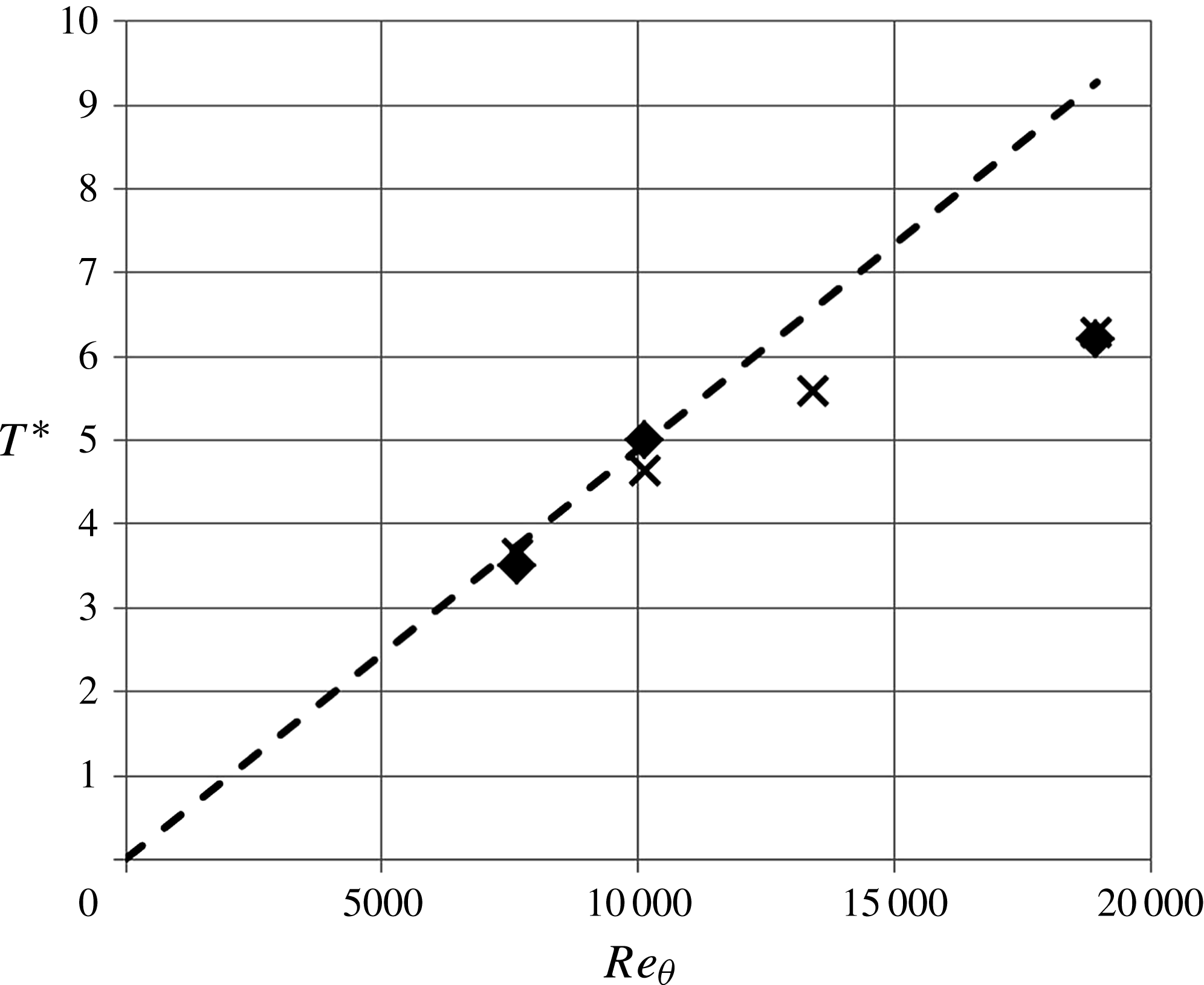
Based on this estimation, the lifetime of the structure scaled in external units should be written as
 $$\begin{eqnarray}T^{\ast }=TU_{e}/{\it\delta}={\it\alpha}\frac{u_{{\it\tau}}^{2}}{{\it\nu}}\frac{{\it\delta}}{U_{e}}.\end{eqnarray}$$
This model is plotted as a dashed line in figure 37. Thanks to the slow variation of
 $\mathit{Re}_{{\it\tau}}$
with respect to
 $\mathit{Re}_{{\it\delta}}$
, the model is linear in the present range and fits the two lowest Reynolds numbers quite well with
 ${\it\alpha}=0.037$
. At the higher Reynolds number, the lifetime of the structure is obviously much shorter than expected from the model. This can be solved empirically by applying a very strong nonlinear correction to the model:
 $$\begin{eqnarray}T^{\ast }=T_{\infty }^{\ast }\tanh \left({\it\beta}\frac{u_{{\it\tau}}^{2}}{{\it\nu}}\frac{{\it\delta}}{U_{e}}\right),\end{eqnarray}$$
with
 ${\it\beta}=0.006$
and
 $T^{\ast }=7$
, an asymptotic value that is expected to be reached at approximately
 $\mathit{Re}_{{\it\theta}}\simeq 40\,000$
.
This simple model has of course no predictive pretentions, except for the fact that it seems to show that, at low Reynolds number, the vortices that are generated at the wall are sparse enough to have very little interaction with each other and, consequently, to have a lifetime proportional to their initial vorticity (like an isolated viscous vortex). When the Reynolds number grows, both convection and the bursting frequency grow so that the number of vortices grows (as evidenced by the high-Reynolds-number DNS of Jiménez Reference Jiménez2013) and nonlinear interactions develop rapidly between these vortices. This seems to limit the lifetime of the hairpin packets. The second interesting fact emerging from this analysis is that there seems to be an asymptotic state reached at approximately
 $\mathit{Re}_{{\it\theta}}\simeq 40\,000$
where
 $T^{\ast }\simeq 7$
. If this is true, it means that the characterization of a fully developed high-Reynolds-number turbulent boundary layer is not out of reach (the Melbourne wind tunnel can reach
 $\mathit{Re}_{{\it\theta}}=50\,000$
).
6. Conclusion
In the present contribution, the space–time pressure–velocity correlations in a turbulent boundary layer at
 $\mathit{Re}_{{\it\theta}}=7300$
, 10 000 and 18 000 were investigated by simultaneous measurements of the fluctuating pressure and velocity.
A static pressure probe and a wall pressure tap were specifically developed for the experiment. Care was taken to achieve a good spatial resolution. The diameter of the pressure tap was about 10 wall units at the highest Reynolds number.
Two stereo PIV planes were placed adjacent to each other in the wall-normal direction to accomplish a field of view large enough to capture a whole boundary layer at once and small enough to identify small-scale structures. The merged field of view corresponded to
 ${\it\delta}\times 0.4{\it\delta}$
in the wall-normal and spanwise directions. The spatial resolution, i.e. the interrogation window size of the PIV analysis, was 50 wall units at the highest Reynolds number.
The fundamental statistics of the velocity, e.g. mean velocity and r.m.s. values of velocity fluctuations, show good agreement with previous studies. The comparison with hot-wire data taken in the same facility by Carlier & Stanislas (Reference Carlier and Stanislas2005) shows that the present stereo PIV measurement provides data of good quality down to
 $y=2~\text{mm}$
, which corresponds to
 $15^{+},25^{+},45^{+}$
for
 $\mathit{Re}_{{\it\theta}}=7300$
, 10 000, 18 000 respectively.
Both the r.m.s. and the PDF of the static pressure fluctuations show good agreement with the measurements by Tsuji et al. (Reference Tsuji, Fransson, Alfredsson and Johansson2007) for
 $\mathit{Re}_{{\it\theta}}=10\,000$
. Slightly larger values of the r.m.s. are observed for the two other Reynolds numbers. This may be due to the fact that the best signal-to-noise ratio was achieved for
 $\mathit{Re}_{{\it\theta}}=10\,000$
. For
 $\mathit{Re}_{{\it\theta}}=7300$
, the turbulent pressure fluctuations are smaller, and for
 $\mathit{Re}_{{\it\theta}}=18\,000$
, the wind-tunnel noise turns out to be relatively larger. This is not a problem for measurement of the pressure–velocity correlations as the noise is mostly acoustic and not correlated with the boundary layer velocity fluctuations. Finally, conditional analysis of the wall pressure as in Thomas & Bull (Reference Thomas and Bull1983) and Johansson et al. (Reference Johansson, Her and Haritonidis1987) shows very comparable behaviour of the conditioned signal.
The 3D space–time pressure–velocity correlations,
 $\boldsymbol{R}_{pu}$
,
 $\boldsymbol{R}_{pv}$
and
 $\boldsymbol{R}_{pw}$
, were evaluated with the fixed pressure probe at the wall and in the field. At the wall, the results are in good agreement with the experimental studies of Thomas & Bull (Reference Thomas and Bull1983), Johansson et al. (Reference Johansson, Her and Haritonidis1987) and Naguib et al. (Reference Naguib, Wark and Juckenhöfel2001) and the DNS results of Del Álamo et al. (Reference Del Álamo, Jiménez, Zandonade and Moser2004). The shape of the correlations obtained seems to indicate that the wall pressure fluctuations are strongly coupled with coherent structures which occupy a large region of the boundary layer (roughly
 $10{\it\delta}/U_{e}\times {\it\delta}\times {\it\delta}$
). Conditioning these correlations on the pressure fluctuation sign splits the full correlation into simpler parts which evidence different phenomena. In both cases, the wall pressure fluctuations appear to be linked to strong and rapid variations of the wall-normal velocity. Streamwise vortical motions of relatively large scales are identified on the sides of the large sweeping and ejection regions at different times of the interaction and at the interface between high and low streamwise velocity regions. In outer scaling, the Reynolds number effect is clearly visible on
 $\boldsymbol{R}_{pu}$
, while
 $\boldsymbol{R}_{pw}$
and
 $\boldsymbol{R}_{pv}$
seem to be less sensitive to this parameter. In general, wall pressure fluctuations of both signs appear to be linked to a strongly organized sweeping motion at the scale of the boundary layer thickness in both the spanwise and wall-normal directions and of the order of
 $3{\it\delta}/U_{e}$
in time. This could correspond to the LSMs identified by several authors (Smits et al.
Reference Smits, Mckeon and Marusic2011). Weaker correlations closer and attached to the wall with a larger extent in time (
 $\simeq 10{-}14{\it\delta}/U_{e}$
) are also observed on
 $\boldsymbol{R}_{pu}$
only, which could be associated with the VLSMs evidenced, for example, by Tomkins & Adrian (Reference Tomkins and Adrian2003), Ganapathisubramani et al. (Reference Ganapathisubramani, Clemens and Dolling2006) and Hutchins & Marusic (Reference Hutchins and Marusic2007).
Looking at the correlations with the fixed pressure point in the inner layer (
 $y/{\it\delta}\leqslant 0.2$
), both
 $\boldsymbol{R}_{pu}$
and
 $\boldsymbol{R}_{pw}$
show an extra region of significant correlation (positive for
 $\boldsymbol{R}_{pu}$
, positive and negative for
 $\boldsymbol{R}_{pw}$
) very elongated in time, which is not observed with the wall pressure. This structure appears to be independent of the one observed at the wall and to grow significantly in time with the Reynolds number in external scaling. It is quite self-similar for the different positions of the fixed pressure point inside the inner layer. In the outer layer, the wall structure disappears and the elongated region evolves significantly up to the boundary layer edge. A comparison of the present
 $\boldsymbol{R}_{pu}$
correlation with the
 $\boldsymbol{R}_{uu}$
one obtained by Tutkun et al. (Reference Tutkun, George, Delville, Stanislas, Johansson, Foucaut and Coudert2009) shows a strong similarity in shape between the two. A possible interpretation is that the elongated structure affecting the field pressure correlation is not located in space at the same place as the sweeping/ejection motions linked to the wall pressure fluctuations.
A comparison of the conditioned wall pressure–velocity correlations presented in movies 7 and 8 with recent results from Ghaemi & Scarano (Reference Ghaemi and Scarano2013) for HAPPs in the near-wall region shows striking similarities for both positive and negative pressure fluctuations. This could be an indication that the LSMs observed in high-Reynolds-number boundary layers are not very different from those associated with the near-wall streaks. This conclusion is supported by an analysis of the correlations obtained with the fixed pressure point in the outer part of the boundary layer, which indicates a possible link with a large ‘hairpin’ (or hairpin packet) type of motion.
One other interesting aspect of the present results is in the comparison with those obtained by Marusic, Mathis & Hutchins (Reference Marusic, Mathis and Hutchins2010) and Mathis, Hutchins & Marusic (Reference Mathis, Hutchins and Marusic2011) on the velocity field. The model developed by these authors clearly shows a relation between the outer large-scale velocity fluctuations and the near-wall ones (which is also visible from the space–time correlations of Tutkun et al. (Reference Tutkun, George, Delville, Stanislas, Johansson, Foucaut and Coudert2009) as shown in figure 35) with only a time delay between them in agreement with the shape of the
 $\boldsymbol{R}_{uu}$
correlation. The present results show that the velocity field influence on both the wall and the field pressure fluctuations is effectively limited to the inside of the boundary layer, but with a significant time extension, much wider than that observed up to now for the velocity field. They seem also to indicate that, sensed by the pressure, there are two main large-scale coherent motions. First, a strong sweeping motion at the scale of the boundary layer which acts mostly on the wall and inner layer pressure fluctuations. Second, as clearly shown by movies 12 and 13, very elongated structures with either large or low streamwise velocity, staggered in span and flanked with large streamwise vortical structures. They are strongly inclined to the wall and influence the pressure fluctuations in the whole boundary layer thickness but not the wall pressure. These elongated structures, of which the low-speed ones have strong similarities with the hairpin packets of Adrian et al. (Reference Adrian, Meinhart and Tomkins2000), can clearly be associated with the VLSMs of Tomkins & Adrian (Reference Tomkins and Adrian2003), Ganapathisubramani et al. (Reference Ganapathisubramani, Clemens and Dolling2006) and Hutchins & Marusic (Reference Hutchins and Marusic2007). They grow significantly in life time (much more than the first one) with the Reynolds number. The overall picture obtained is anyway very similar to the one proposed in the previous century for the very-near-wall region (low- and high-speed streaks with streamwise vortices in between), but now at the scale of the boundary layer. A simplified model of the turbulent boundary layer organization can thus be built with two sets of streaks: the near-wall ones, scaling in wall units, and the outer ones, scaling with
 ${\it\delta}$
in
 $y$
and
 $z$
, both meandering slowly and being tightly linked to streamwise vortical structures of corresponding scale. While the typical size of the near-wall streamwise vortices is of the order of 100 wall units, the lifetime of the outer ones is more of the order of
 $10{\it\delta}/U_{e}$
. The second peak of turbulence, which develops at high Reynolds number away from the wall, can be associated with these outer streamwise elongated vortical structures, by analogy with the near-wall peak of turbulent kinetic energy which is located at a wall distance comparable to the radius of the near-wall streamwise vortices. To complete the model, a large and strong sweeping motion is needed which mostly generates the wall pressure fluctuations and which is probably located between the elongated low- and high-speed structures and linked to the bending of the streamwise vortical structures.
Finally, a simple model seems to indicate that strong nonlinear interactions develop in these elongated streamwise structures when the Reynolds number increases. These interactions limit their lifetime, which could reach an asymptotic value for
 $\mathit{Re}_{{\it\theta}}\simeq 40\,000$
. The question is whether the turbulent boundary layer also reaches an asymptotic state, and whether this new set of streaks is the second one of a quantic cascade, or whether the fact that the structures occupy the whole boundary layer thickness indicates that the canonical high-Reynolds-number turbulent boundary layer state is reached. It is interesting to mention here that
 $\mathit{Re}_{{\it\theta}}\simeq 40\,000$
has already been identified by Stanislas et al. (Reference Stanislas, Perret and Foucaut2008) as a critical value in terms of Reynolds number independence of the ZPG boundary layer characteristics.
Acknowledgements
We thank the ‘Conseil Régional Nord Pas de Calais’ for providing a fellowship to Y. Naka, which allowed this experiment to be performed. The present research work was also supported through the International Campus on Safety and Intermodality in Transportation by the European Community, the Regional Delegation for Research and Technology, the Ministry of Higher Education and Research, and the National Centre for Scientific Research.
Supplementary movies
Supplementary movies are available at http://dx.doi.org/10.1017/jfm.2015.158.
Appendix. Captions of movies
In the present paper, movies 1–13 are provided as extra electronic material to facilitate the understanding of the 3D structure of pressure–velocity correlations. The captions of the movies are listed below.
-
(a) Movie 1: 3D view of conditional wall pressure–streamwise velocity correlation
 $\boldsymbol{R}_{pu}$
for
$p>0$
at
$\mathit{Re}_{{\it\theta}}=10\,000$
. The movie shows the 3D structure of the correlation as follows: 1, oblique view of positive and negative isosurfaces; 2, cut in the
${\rm\Delta}t{-}y$
plane scanning through spanwise locations; 3, cut in the
$y{-}z$
plane at
${\rm\Delta}t=0$
; 4, changing the values of isosurfaces; 5, showing the isosurfaces at different angles.
-
(b) Movie 2: 3D view of conditional wall pressure–streamwise velocity correlation
$\boldsymbol{R}_{pu}$
for
$p<0$
at
$\mathit{Re}_{{\it\theta}}=10\,000$
. The representation is the same as movie 1. -
(c) Movie 3: 3D view of conditional wall pressure–wall-normal velocity correlation
$\boldsymbol{R}_{pv}$
for
$p>0$
at
$\mathit{Re}_{{\it\theta}}=10\,000$
. The representation is the same as movie 1. -
(d) Movie 4: 3D view of conditional wall pressure–wall-normal velocity correlation
$\boldsymbol{R}_{pv}$
for
$p<0$
at
$\mathit{Re}_{{\it\theta}}=10\,000$
. The representation is the same as movie 1. -
(e) Movie 5: 3D view of conditional wall pressure–spanwise velocity correlation
$\boldsymbol{R}_{pw}$
for
$p>0$
at
$\mathit{Re}_{{\it\theta}}=10\,000$
. The representation is the same as movie 1. -
(f) Movie 6: 3D view of conditional wall pressure–spanwise velocity correlation
$\boldsymbol{R}_{pw}$
for
$p<0$
at
$\mathit{Re}_{{\it\theta}}=10\,000$
. The representation is the same as movie 1. -
(g) Movie 7: three components of the conditional wall pressure–velocity correlations represented by colour (
$\boldsymbol{R}_{pu}$
) and vectors (
$\boldsymbol{R}_{pv}$
and
$\boldsymbol{R}_{pw}$
) for
$p>0$
at
$\mathit{Re}_{{\it\theta}}=10\,000$
. The distribution in the
$y{-}z$
plane is scanned within
$-1.5<{\rm\Delta}tU_{e}/{\it\delta}<1$
. -
(h) Movie 8: three components of conditional wall pressure–velocity correlations represented by colour (
$\boldsymbol{R}_{pu}$
) and vectors (
$\boldsymbol{R}_{pv}$
and
$\boldsymbol{R}_{pw}$
) for
$p<0$
at
$\mathit{Re}_{{\it\theta}}=10\,000$
. Distribution in
$y{-}z$
plane is scanned within
$-1<{\rm\Delta}tU_{e}/{\it\delta}<1.5$
. -
(i) Movie 9: 3D view of field pressure–streamwise velocity correlation
$\boldsymbol{R}_{pu}$
at probe position (b:
$y_{p}^{+}=48$
) at
$\mathit{Re}_{{\it\theta}}=10\,000$
. The correlation is Gaussian filtered with a width of
${\it\sigma}^{+}=18.9$
. The representation is the same as movie 1. -
(j) Movie 10: 3D view of field pressure–spanwise velocity correlation
$\boldsymbol{R}_{pw}$
at probe position (b:
$y_{p}^{+}=48$
) at
$\mathit{Re}_{{\it\theta}}=10\,000$
. The correlation is Gaussian filtered with a width of
${\it\sigma}^{+}=18.9$
. The representation is the same as movie 1. -
(k) Movie 11: 3D view of field pressure–spanwise velocity correlation
$\boldsymbol{R}_{pw}$
at probe position (h:
$y_{p}/{\it\delta}=0.55$
) at
$\mathit{Re}_{{\it\theta}}=10\,000$
. The correlation is Gaussian filtered with a width of
${\it\sigma}^{+}=18.9$
. The representation is the same as movie 1. -
(l) Movie 12: three components of the conditional field pressure–velocity correlations at the probe position (c) represented by colour (
$\boldsymbol{R}_{pu}$
) and vectors (
$\boldsymbol{R}_{pv}$
and
$\boldsymbol{R}_{pw}$
) for
$p>0$
at
$\mathit{Re}_{{\it\theta}}=10\,000$
. The distribution in the
$y{-}z$
plane is scanned within
$-2<{\rm\Delta}tU_{e}/{\it\delta}<9$
. -
(m) Movie 13: three components of the conditional field pressure–velocity correlations at the probe position (c) represented by colour (
$\boldsymbol{R}_{pu}$
) and vectors (
$\boldsymbol{R}_{pv}$
and
$\boldsymbol{R}_{pw}$
) for
$p<0$
at
$\mathit{Re}_{{\it\theta}}=10\,000$
. The distribution in the
$y{-}z$
plane is scanned within
$-0.6<{\rm\Delta}tU_{e}/{\it\delta}<5.5$
.