1 Introduction
Turbulent rotating flows are met in a variety of contexts in nature. From the interior of stars, to planet atmospheres and industrial applications, rotation plays a dominant role in determining the properties of the underlying turbulence (Greenspan Reference Greenspan1968; Pedlosky Reference Pedlosky1987; Hopfinger & Heijst Reference Hopfinger and Heijst1993). In its simplest form an incompressible turbulent flow in the presence of rotation is controlled by the incompressible Navier–Stokes equation, which in a rotating frame of reference reads
 $$\begin{eqnarray}\unicode[STIX]{x2202}_{t}\boldsymbol{u}+\boldsymbol{u}\boldsymbol{\cdot }\unicode[STIX]{x1D735}\boldsymbol{u}+2\unicode[STIX]{x1D6FA}\hat{\boldsymbol{e}}_{z}\times \boldsymbol{u}=-\unicode[STIX]{x1D735}P+\unicode[STIX]{x1D708}\unicode[STIX]{x0394}\boldsymbol{u}+\boldsymbol{F},\end{eqnarray}$$
where
 $\boldsymbol{u}$
is the incompressible velocity field,
 $\unicode[STIX]{x1D6FA}$
is the rotation rate (assumed here to be in the
 $z$
direction with
 $\hat{\boldsymbol{e}}_{z}$
its unit vector),
 $P$
is the pressure that enforces the incompressibility condition
 $\unicode[STIX]{x1D735}\boldsymbol{\cdot }\boldsymbol{u}=0$
,
 $\unicode[STIX]{x1D708}$
is the viscosity and
 $\boldsymbol{F}$
is a mechanical body force that acts at some length scale
 $\ell _{f}$
. Traditionally, the strength of turbulence compared to viscous forces is measured by the Reynolds number
 $Re=U\ell _{f}/\unicode[STIX]{x1D708}$
, while compared to the Coriolis force it is measured by the Rossby number
 $Ro=U/(2\unicode[STIX]{x1D6FA}\ell _{f})$
, where
 $U$
stands for the velocity amplitude. Precise definitions of these numbers will be given when we describe in detail the model under study.
It has been known for some time that when rotation is very strong, flows tend to become quasi-two-dimensional (quasi-2D) varying very weakly along the direction of rotation (Hough Reference Hough1897; Proudman Reference Proudman1916; Taylor Reference Taylor1917). The reason for this behaviour is that the incompressible projection of the Coriolis force
 $2\unicode[STIX]{x1D6FA}\hat{\boldsymbol{e}}_{z}\times \boldsymbol{u}-\unicode[STIX]{x1D735}P^{\prime }=2\unicode[STIX]{x1D6FA}\unicode[STIX]{x1D6E5}^{-1}\unicode[STIX]{x2202}_{z}\unicode[STIX]{x1D735}\times \boldsymbol{u}$
does not act on the part of the flow that is invariant along the rotation axis
 $\unicode[STIX]{x2202}_{z}\boldsymbol{u}=0$
. Here
 $P^{\prime }$
is the part of the pressure that enforces incompressibility condition for the Coriolis term and
 $\unicode[STIX]{x1D6E5}^{-1}$
is the inverse laplacian. At the same time velocity fluctuations that vary along this axis become inertial waves that satisfy the dispersion relation,
 $$\begin{eqnarray}\unicode[STIX]{x1D714}_{\boldsymbol{k}}=\pm 2\unicode[STIX]{x1D6FA}\frac{k_{z}}{k},\end{eqnarray}$$
where
 $\unicode[STIX]{x1D714}_{\boldsymbol{k}}$
is the wave frequency,
 $\boldsymbol{k}$
the wavenumber and the sign depends on the helicity of the mode. Fast rotation leads to a de-correlation of inertial waves weakening their interactions. Thus, in the presence of strong rotation, fluid motions that are invariant along the direction of rotation (often referred as the slow manifold) become isolated from the remaining flow, and if forced they dominate, leading to the quasi-2D behaviour (Chen et al.
Reference Chen, Chen, Eyink and Holm2005; Scott Reference Scott2014). This quasi-2D behaviour has been realized in experiments (Ibbetson & Tritton Reference Ibbetson and Tritton1975; Hopfinger, Browand & Gagne Reference Hopfinger, Browand and Gagne1982; Dickinson & Long Reference Dickinson and Long1983; Baroud et al.
Reference Baroud, Plapp, She and Swinney2002, Reference Baroud, Plapp, Swinney and She2003; Ruppert-Felsot et al.
Reference Ruppert-Felsot, Praud, Sharon and Swinney2005; Sugihara, Migita & Honji Reference Sugihara, Migita and Honji2005; Morize & Moisy Reference Morize and Moisy2006; Staplehurst, Davidson & Dalziel Reference Staplehurst, Davidson and Dalziel2008; van Bokhoven et al.
Reference van Bokhoven, Clercx, van Heijst and Trieling2009; Yoshimatsu, Midorikawa & Kaneda Reference Yoshimatsu, Midorikawa and Kaneda2011; Duran-Matute et al.
Reference Duran-Matute, Flór, Godeferd and Jause-Labert2013; Machicoane, Moisy & Cortet Reference Machicoane, Moisy and Cortet2016) and numerical simulations (Yeung & Zhou Reference Yeung and Zhou1998; Godeferd & Lollini Reference Godeferd and Lollini1999; Smith & Waleffe Reference Smith and Waleffe1999; Chen et al.
Reference Chen, Chen, Eyink and Holm2005; Mininni, Alexakis & Pouquet Reference Mininni, Alexakis and Pouquet2009; Thiele & Müller Reference Thiele and Müller2009; Favier, Godeferd & Cambon Reference Favier, Godeferd and Cambon2010; Mininni & Pouquet Reference Mininni and Pouquet2010; Sen et al.
Reference Sen, Mininni, Rosenberg and Pouquet2012; Marino et al.
Reference Marino, Mininni, Rosenberg and Pouquet2013; Alexakis Reference Alexakis2015; Biferale et al.
Reference Biferale, Bonaccorso, Mazzitelli, van Hinsberg, Lanotte, Musacchio, Perlekar and Toschi2016; Valente & Dallas Reference Valente and Dallas2017).
These arguments, however, have various limitations. For large Reynolds numbers
 $Re$
, the quasi-2D behaviour breaks down at scales
 $\ell$
smaller than the Zeman–Hopfinger scale
 $\ell _{Z}$
defined as the scale for which the vorticity
 $w_{\ell }\propto u_{\ell }/\ell$
is comparable to the rotation rate
 $\unicode[STIX]{x1D6FA}$
(Hopfinger et al.
Reference Hopfinger, Browand and Gagne1982; Zeman Reference Zeman1994). Here
 $u_{\ell }$
stands for the typical velocity at scale
 $\ell$
. Thus, for large-Reynolds-number and low-Rossby-number flows, such that
 $1\ll 1/Ro\ll Re$
, the large scales
 $\ell >\ell _{Z}$
show a quasi-2D behaviour, while smaller scales
 $\ell <\ell _{Z}$
display three-dimensional (3D) behaviour. Furthermore, the quasi-2D behaviour is also expected to break down even at large scales for sufficiently elongated boxes
 $H\gg \ell _{f}$
, (where
 $H$
stands for the domain size in the direction of rotation). If
 $H$
is sufficiently large, the slowest inertial mode has a frequency
 $\unicode[STIX]{x1D714}\sim \unicode[STIX]{x1D6FA}\ell _{f}/H$
comparable to or smaller than the inverse of the eddy turnover time
 $\ell /u_{\ell }$
. This last limiting procedure,
 $1\ll 1/Ro\ll H/\ell _{f}$
provided also that
 $Re\gg 1$
, corresponds to the weak wave turbulence limit, in which the nonlinear interactions can be treated in a perturbative manner (Galtier Reference Galtier2003; Nazarenko Reference Nazarenko2011). Finally, for finite (fixed) heights
 $H$
and finite (fixed) Reynolds numbers, fast rotating flows become exactly 2D above a critical rotation rate (Gallet Reference Gallet2015). This corresponds to the limiting procedure
 $Re\ll 1/Ro$
and
 $H/\ell _{f}\ll 1/Ro$
. Thus, in general, the quasi-2D behaviour at low
 $Ro$
depends on the scales under investigation, the geometry of the system, and the relative amplitude of the Rossby and Reynolds number, with different limits leading to different results.
The distinctive difference between 3D and 2D or quasi-2D flows is that the former cascades energy to small scales while the latter cascades energy to large scales. Thus a significant change in the energy balance occurs when the rotation rate is increased and the flow becomes quasi-2D: while in a forward cascade the energy that arrives at small scales gets dissipated, in an inverse cascade the energy piles up at scales of the size of the domain size
 $L$
. Indeed, it has been shown both in numerical simulations (Smith, Chasnov & Waleffe Reference Smith, Chasnov and Waleffe1996; Smith & Waleffe Reference Smith and Waleffe1999; Sen et al.
Reference Sen, Mininni, Rosenberg and Pouquet2012; Pouquet et al.
Reference Pouquet, Sen, Rosenberg, Mininni and Baerenzung2013; Deusebio et al.
Reference Deusebio, Boffetta, Lindborg and Musacchio2014; Biferale et al.
Reference Biferale, Bonaccorso, Mazzitelli, van Hinsberg, Lanotte, Musacchio, Perlekar and Toschi2016) and experiments (Duran-Matute et al.
Reference Duran-Matute, Flór, Godeferd and Jause-Labert2013; Yarom, Vardi & Sharon Reference Yarom, Vardi and Sharon2013; Campagne et al.
Reference Campagne, Gallet, Moisy and Cortet2014; Yarom & Sharon Reference Yarom and Sharon2014; Campagne et al.
Reference Campagne, Gallet, Moisy and Cortet2015, Reference Campagne, Machicoane, Gallet, Cortet and Moisy2016) that while for weak rotation the flow is close to an isotropic state and cascades all energy to the small scales, for fast rotation the flow is in a quasi-2D state that cascades at least part of the energy to the large scales. This quasi-2D state has also been observed in buoyancy-driven systems such as rotating convection (Favier, Silvers & Proctor Reference Favier, Silvers and Proctor2014; Guervilly, Hughes & Jones Reference Guervilly, Hughes and Jones2014; Rubio et al.
Reference Rubio, Julien, Knobloch and Weiss2014; Stellmach et al.
Reference Stellmach, Lischper, Julien, Vasil, Cheng, Ribeiro, King and Aurnou2014; Kunnen et al.
Reference Kunnen, Ostilla-Mónico, van der Poel, Verzicco and Lohse2016; Plumley et al.
Reference Plumley, Julien, Marti and Stellmach2016). This change in the direction of the cascade as a parameter is varied has been the subject of study of various investigations in different systems (Smith & Waleffe Reference Smith and Waleffe1999; Celani, Musacchio & Vincenzi Reference Celani, Musacchio and Vincenzi2010; Alexakis Reference Alexakis2011; Marino et al.
Reference Marino, Mininni, Rosenberg and Pouquet2013; Pouquet & Marino Reference Pouquet and Marino2013; Deusebio et al.
Reference Deusebio, Boffetta, Lindborg and Musacchio2014; Seshasayanan, Benavides & Alexakis Reference Seshasayanan, Benavides and Alexakis2014; Marino, Pouquet & Rosenberg Reference Marino, Pouquet and Rosenberg2015; Sozza et al.
Reference Sozza, Boffetta, Muratore-Ginanneschi and Musacchio2015; Seshasayanan & Alexakis Reference Seshasayanan and Alexakis2016; Benavides & Alexakis Reference Benavides and Alexakis2017). In particular, for rotating flows, it has been shown that the transition from a forward to an inverse cascade happens at critical rotation
 $\unicode[STIX]{x1D6FA}_{c}$
above which the flow starts to cascade part of the injected energy
 $\unicode[STIX]{x1D716}$
inversely at a rate
 $\unicode[STIX]{x1D716}_{inv}$
. The fraction of the rate that cascades inversely
 $\unicode[STIX]{x1D716}_{inv}/\unicode[STIX]{x1D716}$
depends on the difference
 $\unicode[STIX]{x1D6FA}-\unicode[STIX]{x1D6FA}_{c}$
and the height of the domain
 $H$
(Deusebio et al.
Reference Deusebio, Boffetta, Lindborg and Musacchio2014). This description holds at early times before the inverse cascading energy reaches scales the size of the domain. At late times the energy starts to pile up at the largest scale of the system, altering the dynamics. This pile up of energy at the largest scale, amounting to a spectral condensation at the smallest wavenumbers, is referred in the literature as a condensate and has been the subject of many studies on 2D turbulence (Kraichnan Reference Kraichnan1967; Smith & Yakhot Reference Smith and Yakhot1994; Xia et al.
Reference Xia, Punzmann, Falkovich and Shats2008).
In this work, we try to determine the behaviour of a forced rotating flow at late times when the flow has reached a steady state, in the absence of any large-scale dissipative mechanism. Due to the long computational time required to reach a steady state, very few investigations have focused on this regime like the early low-resolution studies in Bartello, Metais & Lesieur (Reference Bartello, Metais and Lesieur1994) and, more recently, the studies in Alexakis (Reference Alexakis2015), Dallas & Tobias (Reference Dallas and Tobias2016), Yokoyama & Takaoka (Reference Yokoyama and Takaoka2017), where turbulent rotating flows at steady state were investigated. Experiments on the other hand, for which long times are realizable, have investigated this steady-state limit (Duran-Matute et al. Reference Duran-Matute, Flór, Godeferd and Jause-Labert2013; Campagne et al. Reference Campagne, Gallet, Moisy and Cortet2014; Yarom & Sharon Reference Yarom and Sharon2014; Campagne et al. Reference Campagne, Machicoane, Gallet, Cortet and Moisy2016; Machicoane et al. Reference Machicoane, Moisy and Cortet2016).
The rest of this paper is structured as follows. In § 2 we present our numerical set-up and introduce our control parameters and observables. In § 3 we discuss possible mechanisms for the saturation of the initial energy growth. In § 4 we present the results on global quantities from the numerical simulations and in § 5 we describe the spatial and spectral structures as well the dynamics involved. In § 6 we discuss the effect of helicity of the forcing on the resulting flow. In § 7 we summarize and draw our conclusions.
2 Numerical set-up, and control parameters
We consider the flow of a unit density liquid in a cubic triple-periodic domain of size
 $2\unicode[STIX]{x03C0}L$
that is in a rotating frame with
 $z$
being the axis of rotation. The governing equation for the flow velocity
 $\boldsymbol{u}$
is given by (1.1). The flow is driven by the body force
 $\boldsymbol{F}$
; here we consider two cases given by
 $$\begin{eqnarray}\boldsymbol{F}=f_{0}\left[\begin{array}{@{}c@{}}-\text{sin}(k_{f}y),\\ +\text{sin}(k_{f}x),\\ \cos (k_{f}x)+\cos (k_{f}y)\end{array}\right]\quad \text{and}\quad \boldsymbol{F}=f_{0}\left[\begin{array}{@{}c@{}}-\text{sin}(k_{f}y),\\ +\text{sin}(k_{f}x),\\ \sin (k_{f}x)+\sin (k_{f}y)\end{array}\right].\end{eqnarray}$$
The first one is maximally helical
 $\langle \boldsymbol{F}\boldsymbol{\cdot }\unicode[STIX]{x1D735}\times \boldsymbol{F}\rangle _{S}=\boldsymbol{k}_{f}\langle \boldsymbol{F}\boldsymbol{\cdot }\boldsymbol{F}\rangle _{S}$
and will be referred to as the helical forcing and the second one has zero helicity
 $\langle \boldsymbol{F}\boldsymbol{\cdot }\unicode[STIX]{x1D735}\times \boldsymbol{F}\rangle _{S}=\mathbf{0}$
and will be referred as the non-helical forcing. Here
 $\langle \rangle _{S}$
denotes spatial average. These forcing functions have been proposed by Roberts (Reference Roberts1972) for dynamo studies and are commonly referred to as Roberts flow. Helicity, defined as
 $H=\langle \boldsymbol{u}\boldsymbol{\cdot }\unicode[STIX]{x1D735}\times \boldsymbol{u}\rangle$
, is known to play an important role in fast-rotating turbulence since it has been shown that its forward cascade can control the dynamics at the small scales (Mininni & Pouquet Reference Mininni and Pouquet2010; Sen et al.
Reference Sen, Mininni, Rosenberg and Pouquet2012). In this work we will examine both cases with and without helicity in parallel. It is also important to note that our forcing is invariant along the axis of rotation, and thus the forcing acts only on the slow manifold (that consists of all the Fourier velocity modes for which
 $k_{z}=0$
). This is in contrast with the case examined in Alexakis (Reference Alexakis2015), Yokoyama & Takaoka (Reference Yokoyama and Takaoka2017), where a Taylor–Green forcing was used that has zero average along the vertical direction. Thus, while the Taylor–Green forcing does not inject energy directly to the slow manifold, the Roberts forcing used here injects energy only to the slow manifold. The two cases can thus be considered as two extremes.
This system was investigated using numerical simulations. All runs were performed using the pseudo-spectral code Ghost (Mininni et al.
Reference Mininni, Rosenberg, Reddy and Pouquet2011), where each component of
 $\boldsymbol{u}$
is represented as a truncated Galerkin expansion in terms of the Fourier basis. The nonlinear terms are initially computed in physical space and then transformed to spectral space using fast Fourier transforms. Aliasing errors are removed using the 2/3 de-aliasing rule. The temporal integration was performed using a fourth-order Runge–Kutta method. Further details on the code can be found in Mininni et al. (Reference Mininni, Rosenberg, Reddy and Pouquet2011). The grid size varied depending on the value of
 $Re_{F}$
and
 $Ro_{F}$
from
 $64^{3}$
to
 $512^{3}$
. A run was considered well resolved if the value of enstrophy spectrum at the cutoff wavenumber was at least one order of magnitude smaller than its value at its peak. Each run started from a random multimode initial condition and was continued for a sufficiently long time that long-time averages in the steady state were obtained.
The parameter
 $f_{0}$
gives the amplitude of the forcing, and
 $k_{f}$
is the wavenumber at which energy is injected into the flow. These two parameters define the length scale
 $\ell _{f}=k_{f}^{-1}$
, the time scale
 $\unicode[STIX]{x1D70F}_{f}=(k_{f}f_{0})^{-1/2}$
and velocity amplitude
 $U_{f}=\sqrt{f_{0}/k_{f}}$
which will be used to non-dimensionalize the control parameters in our system. The product
 $k_{f}L$
gives the scale separation between the forcing scale and the box size. Throughout this work we have fixed the scale separation to
 $k_{f}\,L=4$
. We thus do not investigate the dependence on the box size. The Reynolds number
 $Re_{f}$
and the Rossby number
 $Ro_{f}$
based on
 $U_{f}$
are defined as
 $$\begin{eqnarray}Re_{f}=\frac{\sqrt{f_{0}/k_{f}^{3}}}{\unicode[STIX]{x1D708}}\quad \text{and}\quad Ro_{f}=\frac{\sqrt{f_{0}k_{f}}}{2\unicode[STIX]{x1D6FA}}.\end{eqnarray}$$
The more classical definition of the Reynolds and Rossby number can be obtained using the root-mean-square amplitude of the velocity
 $U=\langle \boldsymbol{u}\boldsymbol{\cdot }\boldsymbol{u}\rangle _{ST}^{1/2}$
, where
 $\langle \cdot \rangle _{ST}$
denotes spatial and temporal average. This leads to the velocity based Reynolds number
 $Re_{u}$
and the velocity based Rossby number
 $Ro_{u}$
,
 $$\begin{eqnarray}Re_{u}=\frac{U}{k_{f}\unicode[STIX]{x1D708}}\quad \text{and}\quad Ro_{u}=\frac{Uk_{f}}{2\unicode[STIX]{x1D6FA}}.\end{eqnarray}$$
In many experiments, as well as in many theoretical arguments, it is the energy injection rate
 $$\begin{eqnarray}\unicode[STIX]{x1D716}=\langle \boldsymbol{u}\boldsymbol{\cdot }\boldsymbol{F}\rangle _{ST}=\unicode[STIX]{x1D708}\langle |\unicode[STIX]{x1D735}\times \boldsymbol{u}|^{2}\rangle _{ST}\end{eqnarray}$$
per unit of volume that is controlled. It is thus worth expressing the control parameters also in terms of
 $\unicode[STIX]{x1D716}$
. This leads to the definition of the Reynolds/Rossby numbers based on
 $\unicode[STIX]{x1D716}$
,
 $$\begin{eqnarray}Re_{\unicode[STIX]{x1D716}}=\frac{\unicode[STIX]{x1D716}^{1/3}}{\unicode[STIX]{x1D708}k_{f}^{4/3}}\quad \text{and}\quad Ro_{\unicode[STIX]{x1D716}}=\frac{\unicode[STIX]{x1D716}^{1/3}k_{f}^{2/3}}{2\unicode[STIX]{x1D6FA}}.\end{eqnarray}$$
Finally, the ratio of the square root of enstrophy to twice the rotation rate is referred to as the micro-Rossby number
 $Ro_{\unicode[STIX]{x1D706}}$
, which in terms of
 $Re_{\unicode[STIX]{x1D716}}$
and
 $Ro_{\unicode[STIX]{x1D716}}$
can be expressed as
 $$\begin{eqnarray}Ro_{\unicode[STIX]{x1D706}}=\frac{\langle |\unicode[STIX]{x1D735}\times \boldsymbol{u}|^{2}\rangle _{ST}^{1/2}}{2\unicode[STIX]{x1D6FA}}=\frac{\unicode[STIX]{x1D716}^{1/2}}{2\unicode[STIX]{x1D708}^{1/2}\unicode[STIX]{x1D6FA}}=Re_{\unicode[STIX]{x1D716}}^{1/2}Ro_{\unicode[STIX]{x1D716}}.\end{eqnarray}$$
In the examined system only
 $(Re_{f},Ro_{f})$
are true control parameters, while
 $(Re_{u},Ro_{u})$
and
 $(Re_{\unicode[STIX]{x1D716}},Ro_{\unicode[STIX]{x1D716}})$
can only be measured a posteriori.
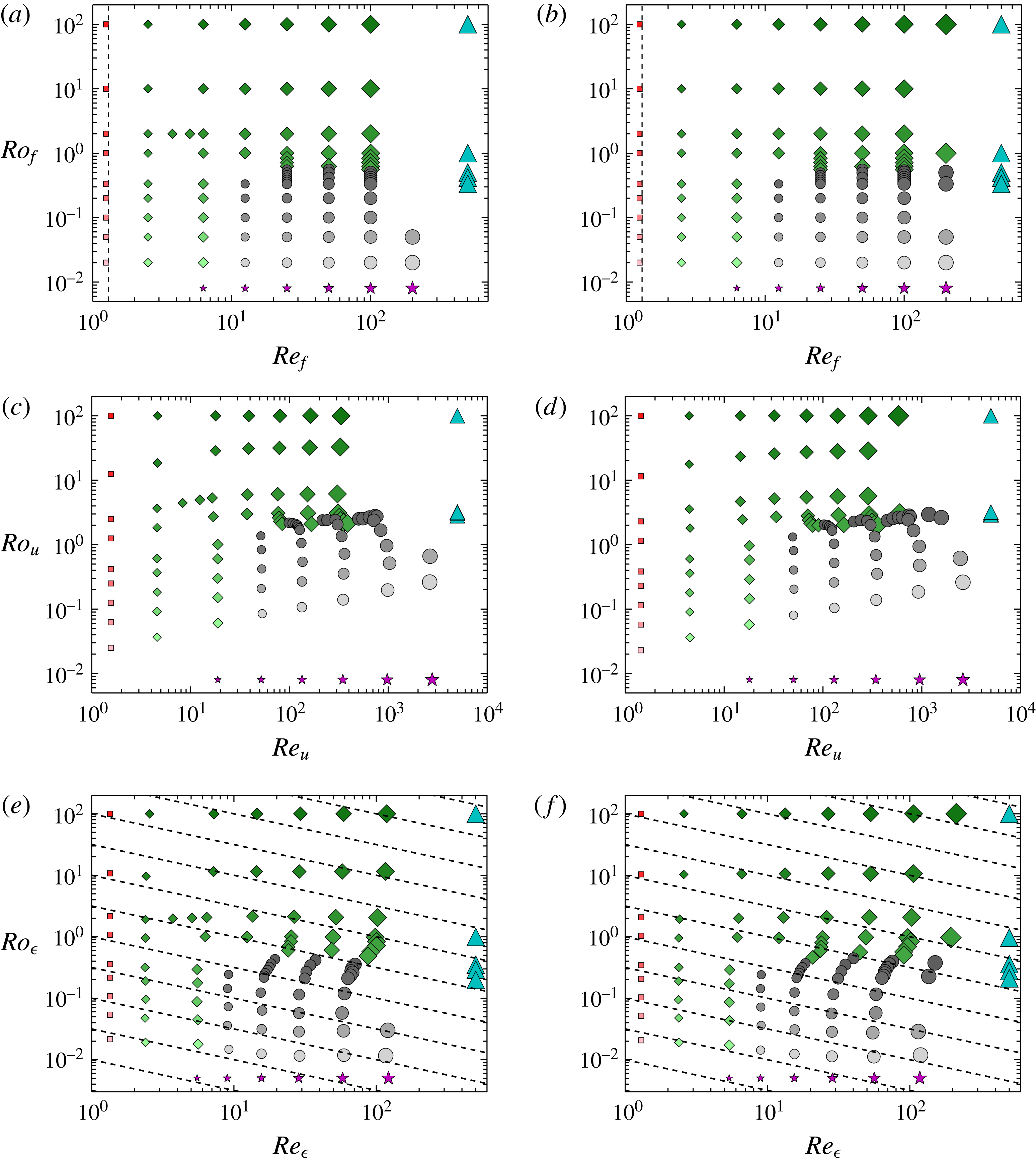
The figures show the location of the numerical runs in the
 $(Ro_{f},Re_{f})$
parameter plane (a,b), the
 $(Ro_{u},Re_{u})$
plane (c,d) and the
 $(Ro_{\unicode[STIX]{x1D716}},Re_{\unicode[STIX]{x1D716}})$
plane (e,f). Helical flows are in (a,c,e) and non-helical flows in (b,d,f). Larger symbols denote larger values of
 $Re_{f}$
and lighter symbols correspond to smaller values of
 $Ro_{f}$
. Different symbols correspond to different behaviour of the flow as follows: squares ▪ (red) correspond to flows that are laminar, diamonds ♦ (green) correspond to unstable or turbulent flows that do not form a condensate, circles ● (black) correspond to turbulent flows that form a condensate, star symbols
 $\star$
(purple) denote the simulations of the reduced two-dimensional equations valid for
 $Ro_{f}\rightarrow 0$
and triangles ▴ (cyan) denote hyperviscous runs.

The location of all of the performed runs in the (
 $Re_{f},Ro_{f}$
) parameter space are shown in figure 1(a,b) for (a) helical flow and (b) non-helical flow in a log–log scale. The figure shows symbols that correspond to simulations that lead to different hydrodynamic steady states. Darker symbols correspond to larger values of
 $Ro_{f}$
while larger symbols correspond to larger values of
 $Re_{f}$
. The largest symbols correspond to simulation runs of size
 $512^{3}$
points. The same symbols, sizes and shades (colours online) are used in some of the subsequent figures and thus the reader can refer to figure 1 to estimate the value of
 $Re_{f}$
and
 $Ro_{f}$
. Each symbol corresponds to different behaviour of the flow: squares ▪ (red) correspond to flows that are laminar, diamonds ♦ (green) correspond to unstable or turbulent flows that do not form a condensate, and circles ● (black) correspond to turbulent flows that form a condensate. We have shifted the points corresponding to
 $\unicode[STIX]{x1D6FA}=0,Ro_{f}=\infty$
to the values
 $Ro_{f}=100$
in order for them to appear along with other points that correspond to finite rotation.
The star symbols
 $\star$
(purple) denote the simulations of the reduced two-dimensional equations valid for
 $Ro_{f}\rightarrow 0$
given by
 $$\begin{eqnarray}\left.\begin{array}{@{}c@{}}\unicode[STIX]{x2202}_{t}\boldsymbol{u}_{2D}+\boldsymbol{u}_{2D}\boldsymbol{\cdot }\unicode[STIX]{x1D735}\boldsymbol{u}_{2D}=-\unicode[STIX]{x1D735}p_{2D}+\unicode[STIX]{x1D708}\unicode[STIX]{x0394}\boldsymbol{u}_{2D}+\boldsymbol{f}_{2D},\\ \unicode[STIX]{x2202}_{t}\boldsymbol{u}_{z}+\boldsymbol{u}_{2D}\boldsymbol{\cdot }\unicode[STIX]{x1D735}u_{z}=+\unicode[STIX]{x1D708}\unicode[STIX]{x0394}u_{z}+\boldsymbol{f}_{z},\end{array}\right\}\end{eqnarray}$$
where
 $\boldsymbol{u}_{2D}$
stands for the horizontal components of the velocity field and
 $u_{z}$
for the vertical. All fields are independent of the vertical coordinate
 $z$
. The points for the 2D simulations (
 $Ro_{f}=0$
limit) are placed at the position
 $Ro_{f}=10^{-2}$
. Finally, the triangles ▴ (cyan) denote hyperviscous runs obtained when we replace the Laplacian in (1.1) with the
 $\unicode[STIX]{x1D6E5}^{4}$
. Hyperviscous runs model the limit
 $Re_{f}\rightarrow \infty$
where a turbulent forward cascade is present. However, in systems like the present one, where inverse cascades build up, the hyperviscous dissipation could affect the amplitude of the large-scale condensate. This is why we only consider the results of hyperviscous runs along with DNS with regular viscosity. They are placed in figure 1 at the value
 $Re_{f}=1000$
.
The vertical dashed line stands for the linear stability boundary of the laminar flow. For the chosen forcing the first unstable mode is
 $z$
-independent and is determined by the linearized version of (2.7). Accordingly the unstable mode is independent of rotation and the vertical component of the laminar flow. As a result the laminar stability boundary is independent of
 $Ro_{f}$
and is the same for the helical and the non-helical flow, that share the same laminar
 $\boldsymbol{u}_{2D}$
at
 $Re_{f}\simeq 1.278$
.
Figure 1(c,d) show the same points in the parameter plane
 $(Re_{u},Ro_{u})$
, with points in the parameter plane
 $(Re_{\unicode[STIX]{x1D716}},Ro_{\unicode[STIX]{x1D716}})$
shown in panels (e,f). The dashed lines in figure 1(e,f) indicate values of constant
 $Ro_{\unicode[STIX]{x1D706}}$
. For the range of examined parameters, compared to the points in the
 $(Re_{f},Ro_{f})$
plane there is a clear shift of the points to larger values of
 $Re_{u}$
as
 $Ro_{u}$
is decreased in figure 1(c,d), while there is a decrease of
 $Re_{\unicode[STIX]{x1D716}}$
as
 $Ro_{\unicode[STIX]{x1D716}}$
is decreased in figure 1(e,f).
Our principal goal in this work is using this large number of numerical simulations to determine the dependence of the large-scale quantities of rotating turbulence such as the saturation amplitude
 $U$
and the energy dissipation rate and to map the different behaviours observed in the parameter space making a phase space diagram.
3 Inverse transfers and saturation of condensates
In this section we present some theoretical estimates for the saturation amplitude of the velocity
 $U$
and the energy dissipation rate
 $\unicode[STIX]{x1D716}$
. As a first step we consider a fixed energy injection rate
 $\unicode[STIX]{x1D716}$
and use (
 $Re_{\unicode[STIX]{x1D716}},Ro_{\unicode[STIX]{x1D716}}$
) as control parameters. We relax this assumption later in the text, where we extend these considerations to the case of fixed forcing amplitude.
For weak rotating and non-rotating systems (
 $Ro\rightarrow \infty$
) the cascade is strictly forward. The external forcing is balanced either by the viscous forces when
 $Re$
is small, or by the nonlinearities that transfer the injected energy to the small scales where viscosity is again effective. These considerations lead to the classical scaling for laminar and turbulent flows between the velocity
 $U$
and the energy injection rate
 $\unicode[STIX]{x1D716}$
,
 $$\begin{eqnarray}U^{2}\propto \unicode[STIX]{x1D716}\frac{\ell _{f}^{2}}{\unicode[STIX]{x1D708}}\quad \text{for}~Re_{\unicode[STIX]{x1D716}}\rightarrow 0\quad \text{and}\quad U^{2}\propto (\unicode[STIX]{x1D716}\ell _{f})^{2/3}\quad \text{for}~Re_{\unicode[STIX]{x1D716}}\rightarrow \infty .\end{eqnarray}$$
Note that both of these scalings are independent of the domain size
 $L$
and the rotation rate
 $\unicode[STIX]{x1D6FA}$
. Using these scalings one can show that for
 $Re_{\unicode[STIX]{x1D716}}\rightarrow \infty$
all the definitions of
 $Re$
given in the previous section are equivalent up to a prefactor so that
 $Re_{\unicode[STIX]{x1D716}}\sim Re_{u}\sim Re_{f}$
and
 $Ro_{\unicode[STIX]{x1D716}}\sim Ro_{u}\sim Ro_{f}$
.
In the presence of an inverse cascade, however, the involved mechanisms for saturation become considerably different, altering these scaling relations. At late times, in order for the system to reach a steady state and saturate the initial increase of the large-scale energy, it has to either suppress the rate at which energy cascades inversely
 $\unicode[STIX]{x1D716}_{inv}$
or to reach sufficiently high amplitudes so that the energy can be dissipated by viscosity. If indeed the transition from forward to an inverse cascade has a critical behaviour, the amplitude of the inverse cascade will depend as a power law on the deviation from criticality
 $Ro_{\unicode[STIX]{x1D716}}^{\ast }$
,
 $$\begin{eqnarray}\unicode[STIX]{x1D716}_{inv}=C_{1}\left(\frac{Ro_{\unicode[STIX]{x1D716}}^{\ast }-Ro_{\unicode[STIX]{x1D716}}}{Ro_{\unicode[STIX]{x1D716}}^{\ast }}\right)^{\unicode[STIX]{x1D6FE}}\unicode[STIX]{x1D716}\quad \text{for}~0<Ro_{\unicode[STIX]{x1D716}}^{\ast }-Ro_{\unicode[STIX]{x1D716}}\ll Ro_{\unicode[STIX]{x1D716}}^{\ast },\end{eqnarray}$$
while away from criticality it is expected that
 $$\begin{eqnarray}\unicode[STIX]{x1D716}_{inv}=C_{2}\,\unicode[STIX]{x1D716}\quad \text{for}~0<Ro_{\unicode[STIX]{x1D716}}\ll Ro_{\unicode[STIX]{x1D716}}^{\ast }.\end{eqnarray}$$
Here
 $Ro_{\unicode[STIX]{x1D716}}^{\ast }$
denotes the critical value of Rossby for which the inverse cascade starts. Note that
 $Ro_{\unicode[STIX]{x1D716}}^{\ast }$
depends on the height of the box but not on the horizontal dimensions (see Deusebio et al.
Reference Deusebio, Boffetta, Lindborg and Musacchio2014). The result in (3.3) holds for the
 $Ro_{\unicode[STIX]{x1D716}}\rightarrow 0$
limit where the flow becomes 2D and
 $\unicode[STIX]{x1D716}_{inv}$
is independent of the rotation rate. The constant
 $C_{2}$
is unity when there is injection of energy only to the horizontal velocity components
 $u_{x},u_{y}$
, while it is between zero and one if
 $u_{z}$
is forced, as is the case we examine here.
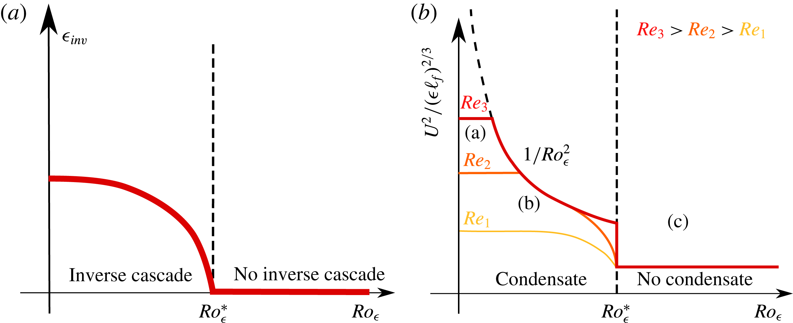
A sketch of the dependence of
 $\unicode[STIX]{x1D716}_{inv}$
on
 $Ro_{\unicode[STIX]{x1D716}}$
is shown in figure 2(a).
(a) Illustration of the expected dependence of the amplitude of the inverse flux
 $\unicode[STIX]{x1D716}_{inv}$
at the early stages of the inverse cascade as a function of the Rossby number
 $Ro_{\unicode[STIX]{x1D716}}$
. (b) Illustration of the expected total energy
 $U^{2}$
as a function of
 $Ro_{\unicode[STIX]{x1D716}}$
at the steady-state regime for different values of
 $Re_{\unicode[STIX]{x1D716}}$
. The dashed vertical line indicates the transition from a flow with no inverse cascade to a flow with an inverse cascade. The dashed curved line shows the scaling
 $1/Ro_{\unicode[STIX]{x1D716}}^{2}$
that reflects the
 $U^{2}\propto \unicode[STIX]{x1D6FA}^{2}L^{2}$
scaling.

The prefactors
 $C_{1}$
and
 $C_{2}\leqslant 1$
and the exponent
 $\unicode[STIX]{x1D6FE}$
have not yet been determined either by DNS or by experiments. In fact, even the conjecture of criticality is very hard to verify with DNS. Although it seems to be plausible, it has been demonstrated with some accuracy only for two-dimensional models (see Seshasayanan et al.
Reference Seshasayanan, Benavides and Alexakis2014; Seshasayanan & Alexakis Reference Seshasayanan and Alexakis2016; Benavides & Alexakis Reference Benavides and Alexakis2017). The reason is that close to the transition point, finite-size and finite-Reynolds effects become important that tend to smooth out the transition. To demonstrate this criticality, ever increasing box sizes and Reynolds numbers need to be considered, and this is extremely costly for three-dimensional simulations. We thus do expect that the transition might not appear as sharp as (3.2) might suggest and the results will be rather dominated by finite size effects that will smooth the transition.
For
 $Ro_{\unicode[STIX]{x1D716}}<Ro_{\unicode[STIX]{x1D716}}^{\ast }$
the energy that arrives at the domain size piles up, forming condensates. In rotating turbulence such condensates can saturate by two possible mechanisms. First, just like in the case of 2D turbulence, saturation comes from viscous forces: the amplitude of the large-scale condensate
 $U_{2D}$
becomes so big that viscous dissipation at large scale balances the rate
 $\unicode[STIX]{x1D716}_{inv}$
that energy arrives at the large scales by the inverse cascade. Thus, the balance
 $\unicode[STIX]{x1D716}_{inv}\propto \unicode[STIX]{x1D708}(U_{2D}^{2}/L^{2})$
is reached. The scaling for the amplitude of the condensate close to the transition point
 $Ro_{\unicode[STIX]{x1D716}}^{\ast }$
thus follows,
 $$\begin{eqnarray}U^{2}\propto C_{1}\frac{\unicode[STIX]{x1D716}L^{2}}{\unicode[STIX]{x1D708}}\left(\frac{Ro_{\unicode[STIX]{x1D716}}^{\ast }-Ro_{\unicode[STIX]{x1D716}}}{Ro_{\unicode[STIX]{x1D716}}^{\ast }}\right)^{\unicode[STIX]{x1D6FE}},\quad \text{for}~0<Ro_{\unicode[STIX]{x1D716}}^{\ast }-Ro_{\unicode[STIX]{x1D716}}\ll Ro_{\unicode[STIX]{x1D716}}^{\ast }.\end{eqnarray}$$
This argument indicates that if the injection rate
 $\unicode[STIX]{x1D716}$
is fixed, the amplitude of the condensate
 $U$
scales supercritically with
 $\unicode[STIX]{x1D6FA}$
with an exponent
 $\unicode[STIX]{x1D6FE}/2$
. For strong rotations away from criticality
 $Ro_{\unicode[STIX]{x1D716}}\ll Ro_{\unicode[STIX]{x1D716}}^{\ast }$
, we expect the scaling for the condensate of 2D turbulence,
 $$\begin{eqnarray}U^{2}\propto C_{2}\frac{\unicode[STIX]{x1D716}L^{2}}{\unicode[STIX]{x1D708}},\quad \text{for}~0<Ro_{\unicode[STIX]{x1D716}}\ll Ro_{\unicode[STIX]{x1D716}}^{\ast }.\end{eqnarray}$$
We will refer to the condensate in this case as a viscous condensate because it is the viscosity that saturates the growth of energy at the large scales.
A different way to saturate the inverse cascade for fast-rotating flows is by breaking the conditions that make the flow quasi-2D. This can happen in domains with periodic boundary conditions, where due to the conservation of vorticity flux the shape of the condensate takes the form of a dipole with one co-rotating vortex and a counter-rotating vortex. Saturation of the inverse transfer of energy can then happen when the counter-rotating vortex cancels locally the rotation rate and energy cascades forward again (see Bartello et al.
Reference Bartello, Metais and Lesieur1994; Alexakis Reference Alexakis2015). This balance is achieved when the eddy turnover time of the condensate
 $L/U$
becomes comparable to the rotation rate
 $\unicode[STIX]{x1D6FA}$
. This leads to the scaling
 $$\begin{eqnarray}U^{2}\propto \unicode[STIX]{x1D6FA}^{2}L^{2}.\end{eqnarray}$$
This scaling was realized in simulations of rotating Taylor–Green flows (see Alexakis Reference Alexakis2015). Note that this scaling is independent of the amplitude of the inverse cascade, and thus independent of the deviation from criticality, that suggest that the transition will be subcritical. This was indeed found to be the case in Alexakis (Reference Alexakis2015). Furthermore, recently Yokoyama & Takaoka (Reference Yokoyama and Takaoka2017) were able to follow the hysteresis diagram of the subcritical bifurcation. Finally, we also note that in this regime a strong asymmetry between co-rotating and counter-rotating vortices is expected, (see, for example, Hopfinger et al. Reference Hopfinger, Browand and Gagne1982; Bartello et al. Reference Bartello, Metais and Lesieur1994; Morize & Moisy Reference Morize and Moisy2006; Bourouiba & Bartello Reference Bourouiba and Bartello2007; Sreenivasan & Davidson Reference Sreenivasan and Davidson2008; Staplehurst et al. Reference Staplehurst, Davidson and Dalziel2008; Van Bokhoven et al. Reference Van Bokhoven, Cambon, Liechtenstein, Godeferd and Clercx2008; Moisy et al. Reference Moisy, Morize, Rabaud and Sommeria2011; Gallet et al. Reference Gallet, Campagne, Cortet and Moisy2014). We will refer to the condensate in this case as a rotating condensate because the energy at the large scales depends on the rotation rate.
From the two mechanisms the one that predicts a smaller value of
 $U_{2D}^{2}$
is going to be more effective. As the Rossby number
 $Ro_{\unicode[STIX]{x1D716}}$
is varied slightly below the critical value, we expect that due to the small amplitude of the inverse cascade, viscosity will be effective in saturating the inverse cascade and the saturation amplitude will be given by (3.4). Away from criticality, however, the breaking of the quasi-2D condition becomes more effective as the amplitude predicted by (3.6) will become smaller than (3.4), and the saturation amplitude will depend on rotation as in (3.6). The region for which the first scaling (3.4) holds becomes smaller as
 $Re_{\unicode[STIX]{x1D716}}$
increases. Thus, in the limit of large
 $Re_{\unicode[STIX]{x1D716}}$
the transition will become discontinuous. Viscosity will become effective again at very small
 $Ro_{\unicode[STIX]{x1D716}}$
where the saturation amplitude will be governed by equation (3.5). The value of
 $Ro_{\unicode[STIX]{x1D716}}$
at which the behaviour transitions from the scaling (3.6) to the scaling (3.5) can be obtained by equating the two predictions. This leads to
 $$\begin{eqnarray}Ro_{\unicode[STIX]{x1D716}}\propto Re_{\unicode[STIX]{x1D716}}^{-1/2},\end{eqnarray}$$
which implies that the transition from a rotating condensate to a viscous condensate occurs when the micro-Rossby number is of order unity
 $Ro_{\unicode[STIX]{x1D706}}=O(1)$
. As we will show in the coming sections, the difference between the two different saturation mechanisms is far from being limited to an abstract scaling. They result in considerable different structures and spectra (as will be shown later in figures 11 and 12).
Figure 2(b) shows a sketch of these expected transitions. The parameter space is thus split into three regions: Region (a), where a condensate forms that is balanced by viscosity for
 $Ro_{\unicode[STIX]{x1D716}}\ll Re_{\unicode[STIX]{x1D716}}^{-1/2}\ll Ro_{\unicode[STIX]{x1D716}}^{\ast }$
, Region (b), in which the condensate that forms equilibrates to a steady state by the counter-rotating vortex cascading energy back to the small scales for
 $Re_{\unicode[STIX]{x1D716}}^{-1/2}\ll Ro_{\unicode[STIX]{x1D716}}<Ro_{\unicode[STIX]{x1D716}}^{\ast }$
, and finally Region (c), where there is no inverse cascade and the system is close to isotropy for
 $Ro_{\unicode[STIX]{x1D716}}>Ro_{\unicode[STIX]{x1D716}}^{\ast }$
. We stress that based on these arguments the behaviour of the flow at large
 $Re_{\unicode[STIX]{x1D716}}$
and low
 $Ro_{\unicode[STIX]{x1D716}}$
depends on the precise order in which the limits
 $Ro_{\unicode[STIX]{x1D716}}\rightarrow 0$
and
 $Re_{\unicode[STIX]{x1D716}}\rightarrow \infty$
are taken.
We now relax the assumption of fixed energy injection rate and consider the case where the system is forced by a constant-in-time forcing of fixed amplitude, as in our simulations. For weak rotation the relation between the forcing amplitude and energy injection rate if the Reynolds number is small is given by
 $$\begin{eqnarray}\unicode[STIX]{x1D716}\propto \frac{f_{0}^{2}\ell _{f}^{2}}{\unicode[STIX]{x1D708}}\quad \text{for}~Re_{f}\ll 1,\quad (\text{laminar}~\text{scaling}),\end{eqnarray}$$
while for large Reynolds numbers we have a viscosity-independent scaling:
 $$\begin{eqnarray}\unicode[STIX]{x1D716}\propto f_{0}^{3/2}\ell _{f}^{1/2}\quad \text{for}~Re_{f}\gg 1,\quad (\text{turbulent}~\text{scaling}).\end{eqnarray}$$
For high rotation rates, however, the injection rate can depend on
 $\unicode[STIX]{x1D6FA}$
if the forcing is not invariant along the axis of rotation. This was shown for the Taylor–Green forcing, where the flow was shown to re-laminarize at high rotation rates (Alexakis Reference Alexakis2015). This effect will not take place in the present investigation, for which the forcing is
 $z$
independent and we thus expect that the scaling in (3.9) remains valid, that along with (3.5) leads to the prediction
 $$\begin{eqnarray}U^{2}\propto U_{f}^{2}Re_{f}(k_{f}L)^{2}\quad \text{for}~Ro_{f}\ll 1,\end{eqnarray}$$
for the amplitude of the condensate. We note that in the presence of large-scale separation this relation is altered to the weaker scaling
 $U^{2}\propto U_{f}^{2}Re_{f}^{2/3}(k_{f}L)^{4/3}$
due to the effect of sweeping (see Shats et al.
Reference Shats, Xia, Punzmann and Falkovich2007; Xia et al.
Reference Xia, Punzmann, Falkovich and Shats2008; Tsang & Young Reference Tsang and Young2009; Gallet & Young Reference Gallet and Young2013). Such an effect, however, is not expected to be present in our case, for which
 $k_{f}L=4$
. For moderate values of
 $Ro_{f}$
, such that the saturation comes from the cancelling of the quasi-2D condition of the counter-rotating vortex,
 $U^{2}$
is independent of the energy injection rate and thus from the forcing amplitude.
 $U^{2}$
is then given by (3.6). Thus, a qualitative difference between the constant injection of energy and constant forcing amplitude is only expected for viscous condensates, and only alters the dependence of the saturation amplitude on
 $Re_{f}$
and not on
 $Ro_{f}$
.
4 Simulation results
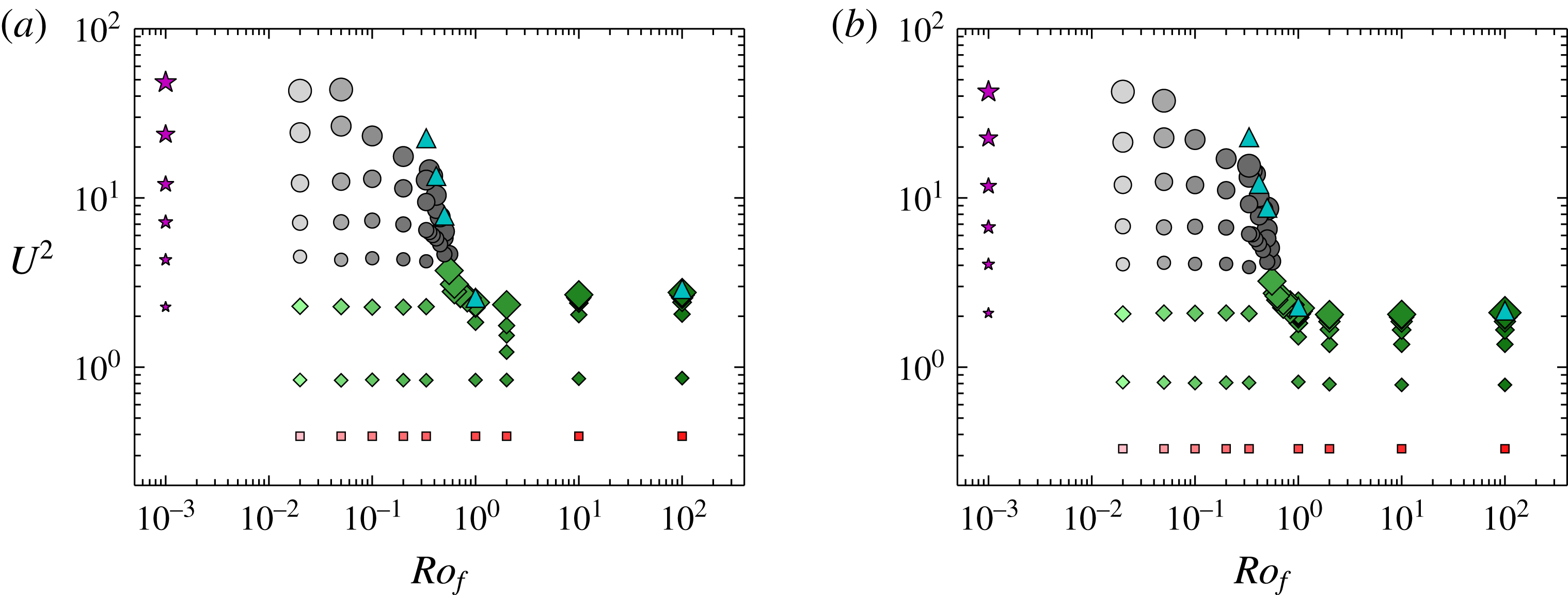
We begin by plotting in figure 3 the square of the velocity saturation amplitude
 $U^{2}$
(in units of
 $U_{f}^{2}$
) as a function of the Rossby number for the entirety of our data points for the helical (a) and the non-helical (b) runs. For both cases the velocity amplitude increases rapidly as
 $Ro_{f}$
decreases beyond a critical value
 $Ro_{f}^{\ast }=O(1)$
. This increase appears to become stronger for larger values of
 $Re_{f}$
(larger symbols). For larger values of
 $Ro_{f}$
(weakly rotating runs),
 $U_{f}^{2}$
quickly saturates to a
 $Ro_{f}$
- and
 $Re_{f}$
-independent value provided
 $Re_{f}$
is sufficiently above the laminar instability threshold.
The figures show the total energy
 $U^{2}$
(in units of
 $U_{f}^{2}$
) as a function of
 $Ro_{f}$
for the examined numerical runs for (a) helical flow and (b) non-helical flow. Larger symbols denote larger values of
 $Re_{f}$
and lighter symbols correspond to smaller values of
 $Ro_{f}$
. Different symbols correspond to different behaviour of the flow as indicated in figure 1.

As we show in what follows, the large increase of
 $U^{2}$
is due to the formation of a condensate at large scales. This is clear for large
 $Re_{f}$
and strong rotation, where
 $Ro_{f}$
is much smaller than the critical value. However, for values of the rotation close to the critical value
 $Ro_{f}^{\ast }$
or for small
 $Re_{f}$
, for which the condensate does not obtain such large values, a better indicator for a condensate formation is the energy
 $U_{2D}^{2}$
contained in the largest Fourier mode
 $|\boldsymbol{k}|=1$
, or in terms of the energy spectrum
 $E_{k}$
we have
 $U_{2D}^{2}=E(k=1)$
, where
 $$\begin{eqnarray}E(k)=\left\langle \int |\hat{\boldsymbol{u}}(\boldsymbol{q})|^{2}\unicode[STIX]{x1D6FF}(|\boldsymbol{q}|-k)\,\text{d}q^{3}\right\rangle \quad \text{with}~\hat{\boldsymbol{u}}(\boldsymbol{q})\equiv \frac{1}{\left(2\unicode[STIX]{x03C0}\right)^{3/2}}\int \boldsymbol{u}\,\text{e}^{\text{i}\boldsymbol{q}\boldsymbol{\cdot }\boldsymbol{x}}\,\text{d}x^{3}.\end{eqnarray}$$
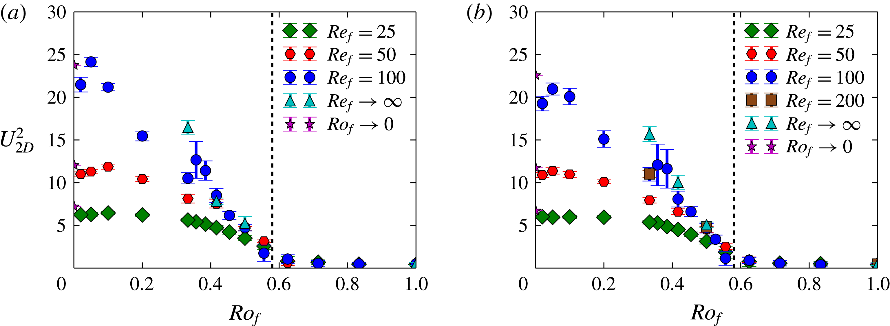
Figure 4 shows
 $U_{2D}^{2}$
as a function of
 $Ro_{f}$
for a few different values of
 $Re_{f}$
for helical and non-helical flow. From this figure the critical value
 $Ro_{f}^{\ast }$
is estimated to be
 $Ro_{f}^{\ast }\simeq 0.6$
for both flows. The value of
 $Ro_{f}^{\ast }$
is denoted by a vertical dashed line in the figures. For values above
 $Ro_{f}^{\ast }$
the large-scale energy remains close to zero. Below
 $Ro_{f}^{\ast }$
the energy
 $U_{2D}^{2}$
increases as
 $Ro_{f}$
decreases further from
 $Ro_{f}^{\ast }$
and asymptotes to a finite value as
 $Ro_{f}\rightarrow 0$
is approached.
The figures show the energy at large scales
 $U_{2D}^{2}$
as a function of
 $Ro_{f}$
(in units of
 $U_{f}^{2}$
) for a few different values of
 $Re_{f}$
for (a) helical flow and (b) non-helical flow. The vertical dashed line at
 $Ro_{f}\sim 0.6$
denotes the critical Rossby number
 $Ro_{f}^{\ast }$
at which the system transitions to a condensate.

Close to the onset the transition to the condensate appears to be supercritical, and
 $U_{2D}^{2}$
can be fitted to a function of the form
 $U_{2D}^{2}\propto C_{3}(Ro_{f}^{\ast }-Ro_{f})^{\unicode[STIX]{x1D6FE}}$
. From the present data we cannot measure with any significant accuracy the exponent
 $\unicode[STIX]{x1D6FE}$
. We note that increasing
 $Re_{f}$
increases the saturation amplitude of
 $U_{2D}^{2}$
, indicating that the prefactor
 $C_{3}$
depends on the Reynolds number. But in the large-
 $Re_{f}$
limit, we see that the data points converge for
 $Ro_{f}$
close to
 $Ro_{f}^{\ast }$
. This shows that, unlike the discussion in § 3 and the results of Alexakis (Reference Alexakis2015) and Yokoyama & Takaoka (Reference Yokoyama and Takaoka2017), the transition at large
 $Re_{f}$
is supercritical.
The figures show the product
 $U_{2D}Ro_{f}$
(in units of
 $U_{f}$
) as a function of
 $Ro_{f}$
for a few different values of
 $Re_{f}$
for (a) helical flow and (b) non-helical flow. The vertical dashed line at
 $Ro_{f}\sim 0.6$
denotes the critical Rossby number for the transition to condensates. The horizontal dashed line denotes the scaling
 $U_{2D}Ro_{f}\sim 1$
.

For intermediate values of
 $Ro_{f}$
and for sufficiently large values of
 $Re_{f}$
, we are expecting that
 $U_{2D}^{2}$
will saturate to values that follow the scaling of the rotating condensates
 $U_{2D}\propto \unicode[STIX]{x1D6FA}L$
(3.6), that implies that the saturation amplitude is such that
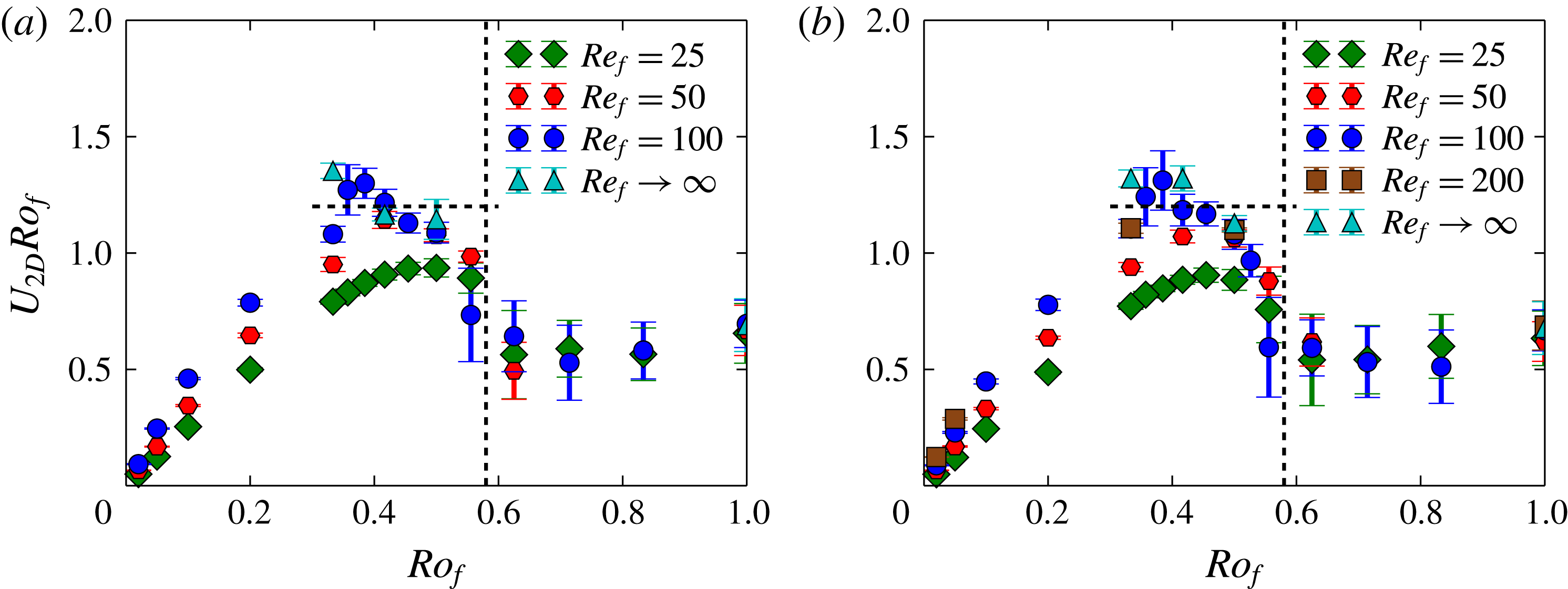
 $U_{2D}Ro_{f}\simeq 1$
. To test this expectation in figure 5 we plot
 $U_{2D}Ro_{f}$
as a function of
 $Ro_{f}$
for different values of
 $Re_{f}$
. Indeed in the region
 $0.3>Ro_{f}>Ro_{f}^{\ast }$
the product
 $U_{2D}Ro_{f}$
appears to converge to an order one value as
 $Re_{f}$
is increased, independent of
 $Ro_{f}$
. We note that the largest
 $Re_{f}$
points are close to the hyperviscous results, implying independence on
 $Re_{f}$
has been reached. Although the results indicate that the saturation mechanism leading to (3.6) is plausible, the range of validity is too small to claim that the scaling has been demonstrated.
To extend the range of validity to smaller values of
 $Ro_{f}$
we need to extend our simulations to larger values of
 $Re_{f}$
. However, this becomes numerically very costly, not only because it implies an increase of resolution, but also because the saturation amplitude of the condensate becomes large, and the time scale to reach saturation increases. As an example we mention that if we would like to extend the range of the rotating condensate to a value of
 $Ro_{\unicode[STIX]{x1D716}}$
half as small, it will require achieving a
 $Re_{\unicode[STIX]{x1D716}}$
that is four times as large as the one used now. This would require a spatial grid that is
 $4^{3/4}$
finer in each direction. If we take in to account the computational cost increase due to the CFL condition (Courant, Friedrichs & Lewy Reference Courant, Friedrichs and Lewy1928) by a factor of
 $2\times 4^{3/4}$
(due to the finer grid and twice larger
 $U$
) and the twice longer duration of the run to attain saturation, we arrive at a computational cost that is
 $2^{8}$
times more expensive than the present computations.
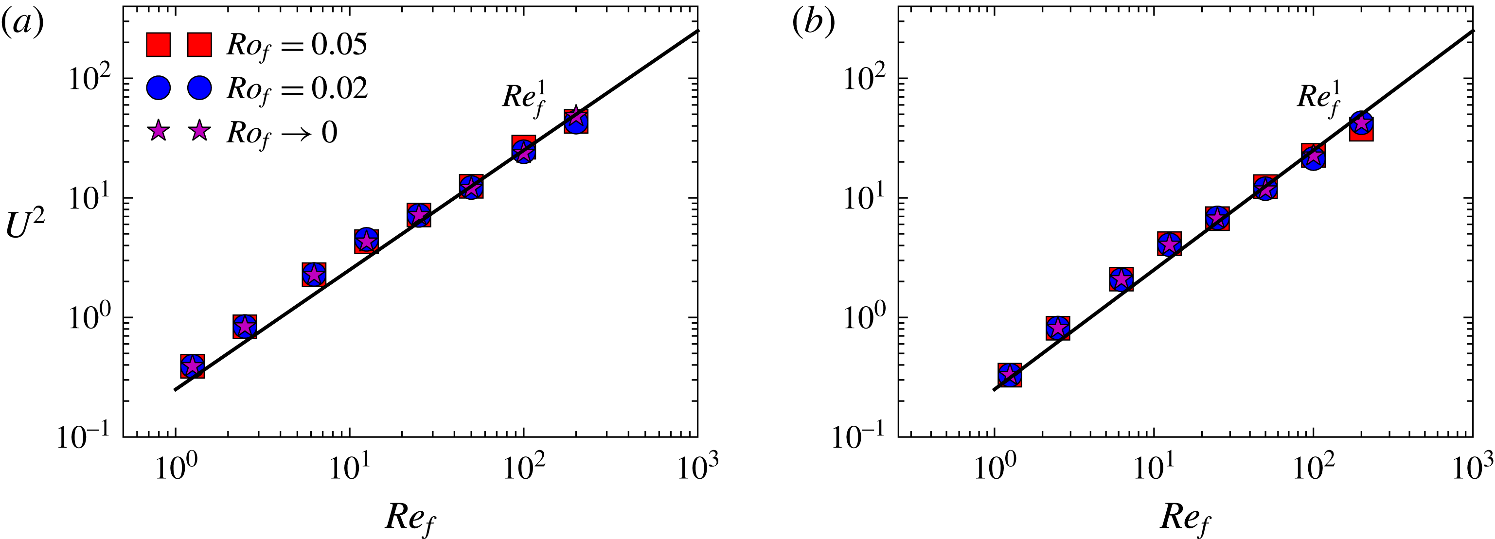
The figures show the energy
 $U^{2}$
(in units of
 $U_{f}^{2}$
) as a function of
 $Re_{f}$
for very small values of
 $Ro_{f}\ll 1$
for (a) helical flow and (b) non-helical flow. The thick line denotes the linear scaling with
 $Re_{f}$
.

Finally, in figure 4, for very small values of
 $Ro_{f}$
the energy
 $U_{2D}^{2}$
asymptotes to a finite value. This value matches the results obtained from the 2D simulations using equation (2.7) that are marked by a star, indicating that the flow has become two-dimensional. The saturation amplitude
 $U_{2D}^{2}$
at the
 $Ro_{f}\rightarrow 0$
limit, however, depends on the value of
 $Re$
. In figure 6 we plot
 $U^{2}$
for the smallest values of
 $Ro_{f}$
examined as a function of
 $Re_{f}$
, along with the results from the system (2.7). The data scale linearly with
 $Re_{f}$
in agreement with the prediction given in (3.10) for the viscous condensate. Equating the two results shown in figures 5 and 6, we obtain that the transition from the rotating condensate regime to the viscous condensate regime occurs when
 $Ro_{f}^{-2}\sim Re_{f}$
, as seen in (3.7).
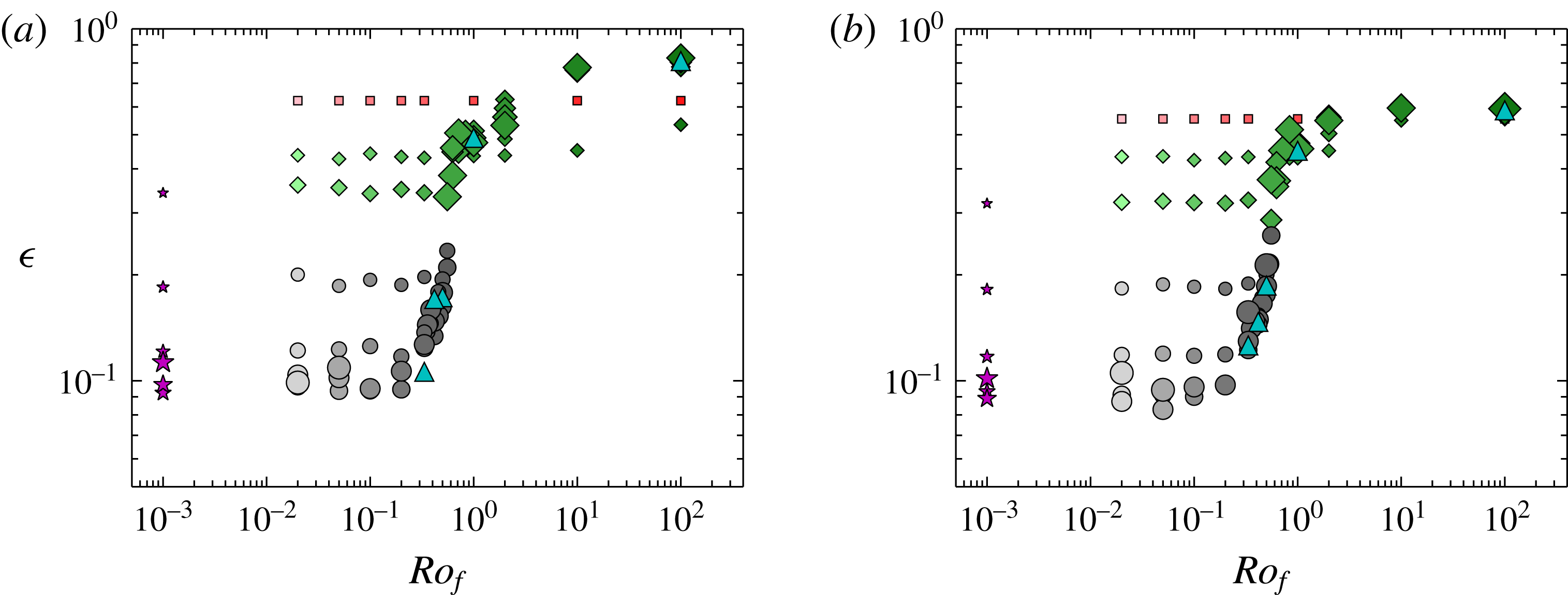
The figures show the injection/dissipation rate
 $\unicode[STIX]{x1D716}$
(in units of
 $U_{f}^{3}k_{f}$
) as a function of
 $Ro_{f}$
for the examined numerical runs for (a) helical flow and (b) non-helical flow. Larger symbols denote larger values of
 $Re_{f}$
and lighter symbols correspond to smaller values of
 $Ro_{f}$
. Different symbols correspond to different behaviour of the flow as indicated in figure 1.

We now focus on the effect of rotation on the energy injection rate in the system. In figure 7 we plot the energy injection rate
 $\unicode[STIX]{x1D716}$
(in units of
 $f_{0}^{3/2}k_{f}^{1/2}$
) as a function of
 $Ro_{f}$
for the entirety of our data points for the helical (a) and the non-helical (b) runs. We remind the reader that smaller symbols indicate smaller Reynolds numbers as in figure 1. The energy dissipation rate saturates to a value independent of
 $Re_{f}$
in the large-
 $Re_{f}$
limit. This value, however, is different for small and large values of
 $Ro_{f}$
, with the transition occurring over a thin region close to
 $Ro_{f}=Ro_{f}^{\ast }$
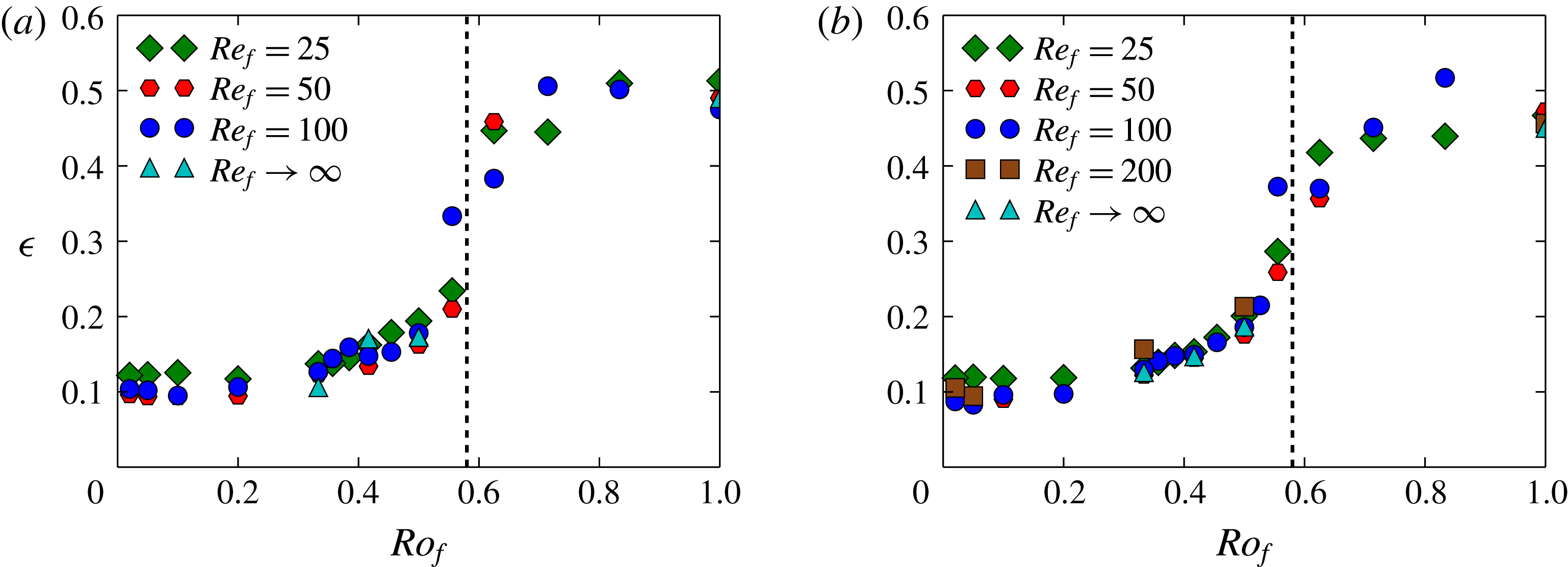
. This is seen more clearly in figure 8, where we have concentrated on the five largest values of
 $Re_{f}$
and plotted the data in a linear scale close to
 $Ro_{f}^{\ast }$
. For these values of
 $Re_{f}$
, the energy injection rate is decreased by a factor of five as
 $Ro_{f}$
is decreased. The decrease in the value of
 $\unicode[STIX]{x1D716}$
as
 $Ro_{f}$
is decreased occurs very fast when
 $Ro_{f}$
is close to its critical value
 $Ro_{f}^{\ast }=0.6$
. The transition by this sudden jump at
 $Ro_{f}^{\ast }$
indicates that, possibly close to the critical point, the dependence of
 $\unicode[STIX]{x1D716}$
on
 $Ro_{f}$
could be discontinuous. Another possibility is that
 $\unicode[STIX]{x1D716}$
is continuous but with diverging derivatives close to the critical point. Similar behaviour has been observed close to the transition to an inverse cascade for a two-dimensional magnetohydrodynamic flow where the low dimensionality of the system allowed a much closer investigation. In any case the investigation of the energy injection close to the critical rotation rate is very interesting but would require long runs that are expensive for numerical simulations but could be addressed more easily with experiments.
The figures show the dissipation rate
 $\unicode[STIX]{x1D716}$
(in units of
 $U_{f}^{3}k_{f}$
) as a function of
 $Ro_{f}$
for a few different values of
 $Re_{f}$
for (a) helical flow and (b) non-helical flow. The vertical dashed line at
 $Ro_{f}\sim 0.6$
denotes the critical Rossby number for the transition to a condensate.

We conclude this section by considering the ratio
 $\unicode[STIX]{x1D716}/(U^{3}k_{f})$
. The quantity
 $\unicode[STIX]{x1D716}/(U^{3}k_{f})$
is sometimes referred to as the drag coefficient. For laminar flows it scales like
 $1/Re_{u}$
, while it tends to a non-zero constant for strongly turbulent flows at large
 $Re_{u}$
. The finite asymptotic value of this ratio at large
 $Re_{u}$
gives one of the fundamental assumptions of turbulence theory, that of finite dissipation at the zero-viscosity limit. This has been clearly demonstrated in experiments of non-rotating turbulence and large-scale numerical simulations (see Sreenivasan Reference Sreenivasan1984; Kaneda et al.
Reference Kaneda, Ishihara, Yokokawa, Itakura and Uno2003; Ishihara et al.
Reference Ishihara, Morishita, Yokokawa, Uno and Kaneda2016). In rotating turbulence experiments it has been investigated in Campagne et al. (Reference Campagne, Machicoane, Gallet, Cortet and Moisy2016), where the drag coefficient has been shown to scale as
 $Ro_{u}$
for sufficiently small
 $Ro_{u}$
. We note that in their experimental set-up it was the velocity of the propellers that were used to define
 $Ro_{u}$
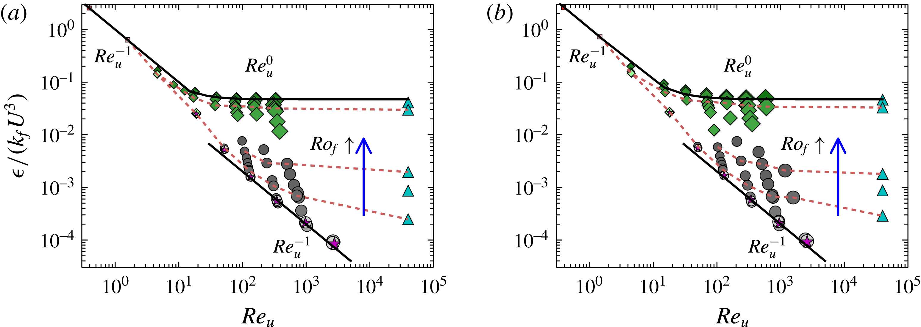
. In figure 9 we plot the ratio
 $\unicode[STIX]{x1D716}/(U^{3}k_{f})$
as a function of
 $Re_{u}$
for different Rossby numbers. The arrow indicates the direction that
 $Ro_{f}$
is increased (i.e. rotation is decreased). The dashed lines connect points with the same value of
 $Ro_{f}$
for three different values of
 $Ro_{f}=1.0,0.5,0.33$
as we move from top to bottom.
The figures show the normalized dissipation rate
 $\unicode[STIX]{x1D716}/(U^{3}k_{f})$
as a function of
 $Re_{u}$
for the examined numerical runs for (a) helical flow and (b) non-helical flow. Larger symbols denote larger values of
 $Re_{f}$
and lighter symbols correspond to smaller values of
 $Ro_{f}$
. Different symbols correspond to different behaviour of the flow as indicated in figure 1. The thick lines denote the laminar scaling
 $Re_{u}^{-1}$
and the turbulent scaling
 $Re_{u}^{0}$
. The blue vertical arrow indicates the direction of increasing
 $Ro_{f}$
(decreasing
 $\unicode[STIX]{x1D6FA}$
). The three dashed brown lines connect the data points of three values
 $Ro_{f}=1.0,0.5,0.33$
as we move from top to bottom.

For rotation rates such that
 $Ro_{f}>Ro_{f}^{\ast }$
(diamonds), the data show a
 $Re_{u}^{-1}$
scaling at low
 $Re_{u}$
that transitions to a constant at large
 $Re_{u}$
demonstrating a finite dissipation at infinite
 $Re_{u}$
. This asymptotic value decreases slightly with
 $Ro_{f}$
. For the runs with
 $Ro_{f}<Ro_{f}^{\ast }$
(circles) on the other hand, the region of the laminar scaling
 $Re_{u}^{-1}$
appears to extend to larger values of
 $Re_{u}$
. The very fast rotating runs (circles with light colours) and the
 $2D$
simulations from (2.7) show a
 $Re_{u}^{-1}$
scaling throughout the examined range. The prefactor in front of
 $Re_{u}^{-1}$
has decreased at the condensate regime because the laminar vortices are at the scale of the forcing (3.1) while the viscous condensate vortices are at the scale of the box size (3.5). However, for fixed
 $Ro_{f}$
(dashed lines), as the Reynolds number is increased the
 $Re_{u}^{-1}$
scaling appears to flatten to a
 $Re_{u}$
-independent scaling. This occurs for the flows that are in the rotating condensate regime. This suggests that even for the rotating runs, the ratio
 $\unicode[STIX]{x1D716}/(U^{3}k_{f})$
will reach an asymptotic non-zero value at
 $Re_{u}\rightarrow \infty$
(for fixed
 $Ro_{f}$
) matching the one obtained by the hyperviscous simulations. This asymptotic value, however, is different for different values of
 $Ro_{f}$
, indicating that the value of the drag coefficient depends on the Rossby number.
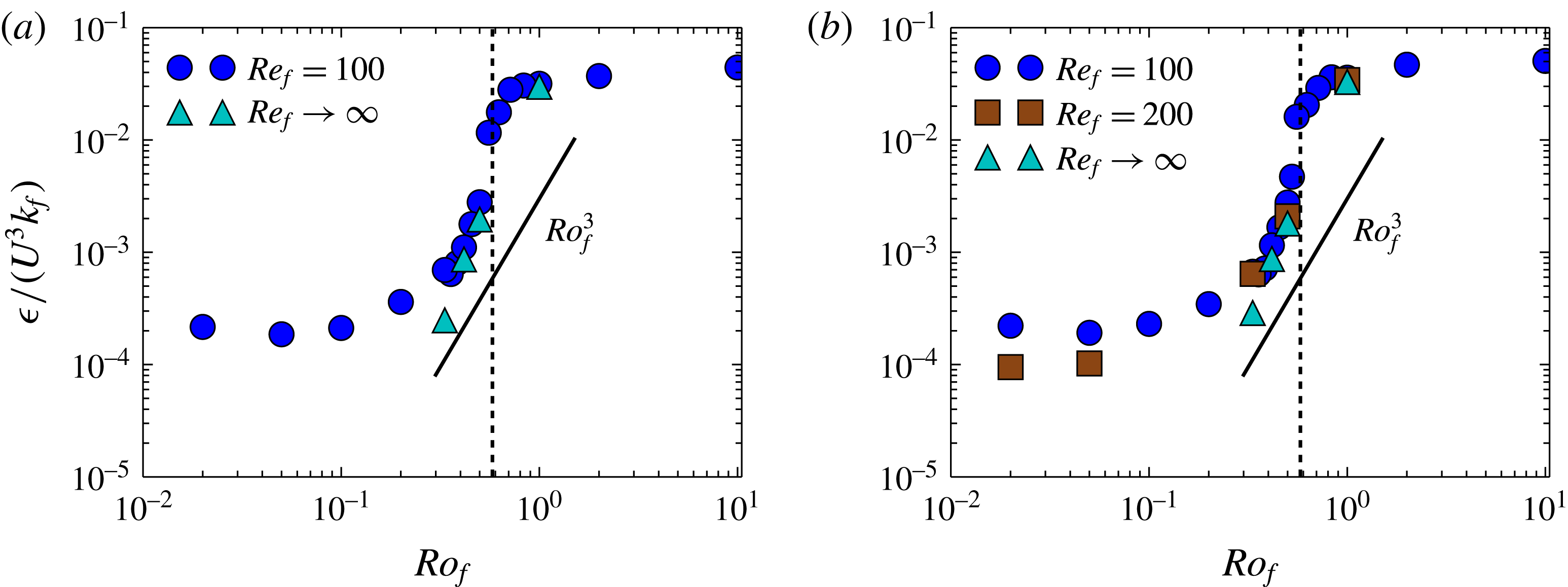
The values of this asymptotic behaviour along with the results of the hyperviscous runs are shown in figure 10, where
 $\unicode[STIX]{x1D716}/(U^{3}k_{f})$
is plotted as a function of
 $Ro_{f}$
. The results are compared with the scaling
 $\unicode[STIX]{x1D716}/(U^{3}k_{f})\propto Ro_{f}^{3}$
. This scaling is obtained by assuming a constant injection rate and a saturation amplitude that follows
 $U\propto \unicode[STIX]{x1D6FA}L$
. The data appear to be slightly steeper. Perhaps this is not surprising considering the small range of
 $Ro_{f}$
in which the scaling
 $U\propto \unicode[STIX]{x1D6FA}L$
was shown to hold in figure 5. Note that weak wave turbulence predicts the scaling
 $\unicode[STIX]{x1D716}/(U^{3}k_{f})\propto Ro_{\unicode[STIX]{x1D716}}$
, which is clearly not obtained here. We note also that the scaling
 $\unicode[STIX]{x1D716}/(U^{3}k_{f})\propto Ro$
was also obtained in the experiments of Campagne et al. (Reference Campagne, Machicoane, Gallet, Cortet and Moisy2016); however, not due to weak wave turbulence but due to a two-dimensionalization of the large-scale flow. The difference with the present scaling could be due to boundary layer effects that are absent in our simulations.
The figures show the normalized dissipation rate
 $\unicode[STIX]{x1D716}/(U^{3}k_{f})$
as a function of
 $Ro_{f}$
for a few different values of
 $Re_{f}\gg 1$
for (a) helical flows and (b) non-helical flows. The thick line denotes the scaling
 $Ro_{f}^{3}$
and the vertical dashed line denotes the critical Rossby number for the transition to condensates.

5 Structures, spectra and dynamical behaviour
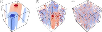
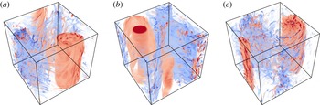
In this section we try to obtain an understanding of the results in the previous section by visualizing the structures involved and examining their spectral and temporal behaviour. We start by the visualization of the flows. Figure 11 shows colour-coded visualizations of the vertical vorticity field. The red colours correspond to vorticity parallel to rotation while the blue colours correspond to vorticity antiparallel to rotation. The three images have been constructed from numerical simulations corresponding to the three regimes discussed in the previous section (in figure 2
b)): panel (a) shows the viscous condensate, panel (b) shows the rotating condensate with the counter-rotating vortex cascading energy back to the small scales and (c) shows the weakly rotating (or non-rotating) turbulence. In the first case (panel a) the flow looks very close to a 2D state with no visible variations along the
 $z$
direction and no observed asymmetry between co-rotating and counter-rotating vortices. In the second case (panel b) a condensate is also formed, but only clearly observed for the co-rotating vortex. The counter-rotating vortex, although present, is infested with small-scale eddies that extract energy from it. Finally, in the third case (panel c), no large-scale condensate is observed and the flow looks isotropic.
The figures show the contours of the vertical vorticity
 $\unicode[STIX]{x1D714}_{z}$
for (a)
 $Ro_{f}=0.02,Re_{f}=100$
(viscous condensate), (b)
 $Ro_{f}=0.5,Re_{f}=100$
(rotating condensate), (c)
 $Ro_{f}=\infty ,Re_{f}=100$
(3D turbulence). Red colours correspond to positive vorticity and blue colours correspond to negative vorticity.

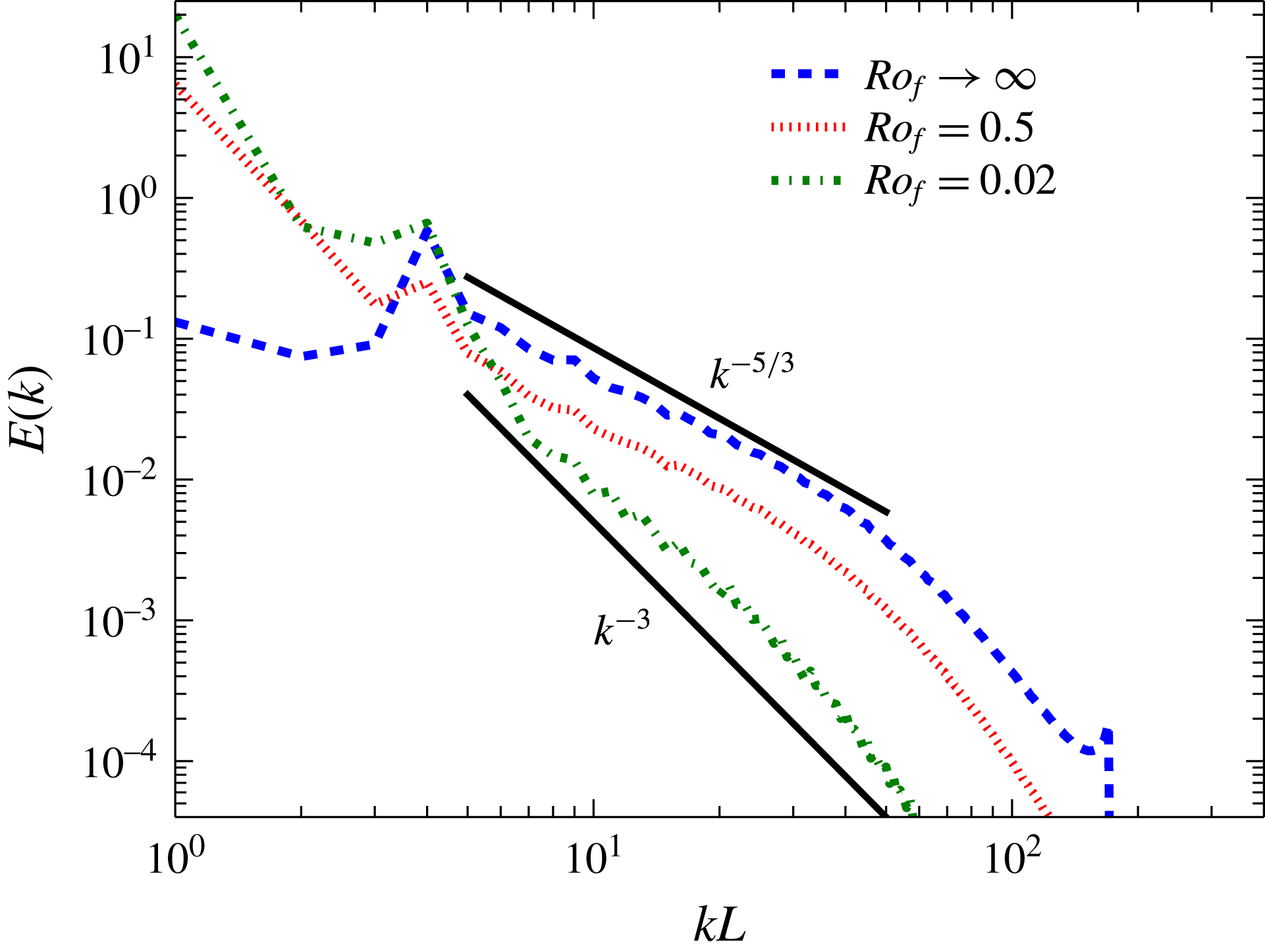
The spectra for the three cases are shown in figure 12. The spectrum for the flow in the viscous condensate regime is shown with a green dash-dot line. The energy is concentrated at the smallest wavenumber
 $kL=1$
, with the energy for wavenumbers above
 $k_{f}L=4$
dropping very fast. In the non-rotating case, shown by a dashed line, energy is concentrated at the forcing wavenumber
 $k_{f}L=4$
that is followed by a power-law spectrum close to
 $k^{-5/3}$
. Finally, the case in the intermediate regime, shown by the dotted line, shows signs of both behaviours: the energy is concentrated at the largest scale
 $kL=1$
as in the viscous condensate case but the spectrum at the small scales follows a
 $k^{-5/3}$
power law as in the non-rotating case. Thus, the spectrum for the rotating condensate is in agreement with the coexistence of a condensate along with a forward cascade. The temporal energy spectra in fast-rotating flows have been measured in experiments as well (see Duran-Matute et al.
Reference Duran-Matute, Flór, Godeferd and Jause-Labert2013; Campagne et al.
Reference Campagne, Gallet, Moisy and Cortet2015, Reference Campagne, Machicoane, Gallet, Cortet and Moisy2016) although the different forcing mechanisms and absence of a Taylor hypothesis for the large scales makes it difficult to make a one-to-one comparison with the ones presented here. An obvious extension of the present work is the calculation of spatio-temporal spectra that allow one to make the connection between the two (di Leoni, Cobelli & Mininni Reference di Leoni, Cobelli and Mininni2015; Clark di Leoni & Mininni Reference Clark di Leoni and Mininni2016).
The figure shows the energy spectra for a few different values of
 $Ro_{f}$
with
 $Re_{f}=100$
. The black thick lines denote the scaling
 $k^{-5/3},k^{-3}$
.

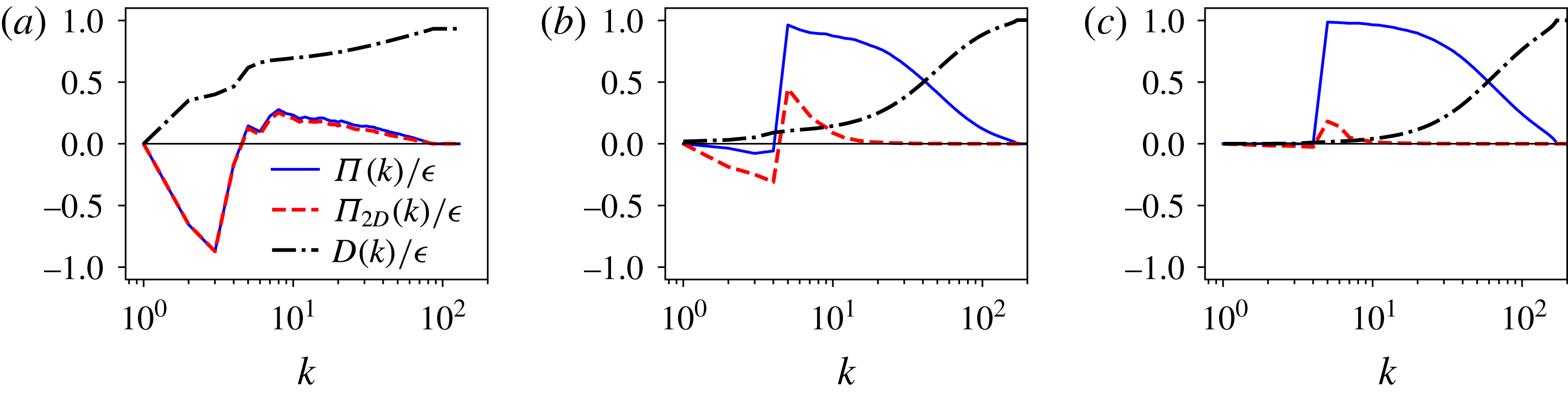
The processes for upscale and downscale cascade are shown more clearly in figure 13, where the normalized energy flux
 $\unicode[STIX]{x1D6F1}(k)/\unicode[STIX]{x1D716}$
, the normalized 2D energy flux
 $\unicode[STIX]{x1D6F1}_{2D}(k)/\unicode[STIX]{x1D716}$
and the normalized scale-dependent dissipation rate
 $D(k)/\unicode[STIX]{x1D716}$
are shown for three different cases: figure 13(a) for the viscous condensate regime, figure 13(b) for the rotating condensate and figure 13(c) for 3D turbulent case with no rotation. The energy fluxes
 $\unicode[STIX]{x1D6F1}(k),\unicode[STIX]{x1D6F1}_{2D}(k)$
and the scale-dependent dissipation rate
 $D(k)$
are defined as
 $$\begin{eqnarray}\unicode[STIX]{x1D6F1}(k)=\langle \boldsymbol{u}_{k}^{{<}}\boldsymbol{\cdot }(\boldsymbol{u}\boldsymbol{\cdot }\unicode[STIX]{x1D735}\boldsymbol{u})\rangle ,\quad \unicode[STIX]{x1D6F1}_{2D}(k)=\langle \overline{\boldsymbol{u}}_{k}^{{<}}\boldsymbol{\cdot }(\overline{\boldsymbol{u}}\boldsymbol{\cdot }\unicode[STIX]{x1D735}\overline{\boldsymbol{u}})\rangle ,\quad D(k)=\unicode[STIX]{x1D708}\mathop{\sum }_{|k^{\prime }|<k}(k^{\prime })^{2}E(k^{\prime }),\end{eqnarray}$$
where
 $\boldsymbol{u}_{k}^{{<}}(x)$
stands for the filtered velocity so that only Fourier modes with wavenumbers of norm less than
 $k$
are kept and the over-bar stands for vertical average. In the 3D-turbulence case, shown in figure 13(c), all the energy cascades to the small scales and the dissipation is concentrated at the smallest scales. In the rotating condensate, shown in figure 13(b), the 2D flux
 $\unicode[STIX]{x1D6F1}_{2D}(k)$
is negative at large scales, indicating that the 2D motions transfer part of the energy to large scales sustaining the condensate. However, the net energy cascade to the large scales remains close to zero, as seen from
 $\unicode[STIX]{x1D6F1}(k)$
, implying that the remaining (not 2D) interactions bring the energy transferred to large scales by
 $\unicode[STIX]{x1D6F1}_{2D}$
back to the small scales in a flux loop mechanism. Similar flux loop mechanisms have been observed in 2D stratified turbulence (Boffetta et al.
Reference Boffetta, De Lillo, Mazzino and Musacchio2011) and compressible 2D turbulence (Falkovich & Kritsuk Reference Falkovich and Kritsuk2017). In this case the dissipation is seen to be concentrated at the small scales. Finally, in the case of the viscous condensate (figure 13
a), the 2D flux
 $\unicode[STIX]{x1D6F1}_{2D}(k)$
takes most of the energy to large scales, where it is dissipated. In the large scales the flux is negative and there is also a weak forward cascade to small scales, as seen from
 $\unicode[STIX]{x1D6F1}(k)$
, possibly related to the vertical velocity component whose related energy cascades forward. The total energy flux
 $\unicode[STIX]{x1D6F1}(k)$
is almost identical to the 2D flux
 $\unicode[STIX]{x1D6F1}_{2D}(k)$
, implying that 3D effects are absent. The dissipation at the large scales is much larger than the previous cases, with more than half the total dissipation occurring at scales equal to and larger than the forcing scale.
The figures show the normalized energy flux
 $\unicode[STIX]{x1D6F1}(k)/\unicode[STIX]{x1D716}$
, the normalized 2D energy flux
 $\unicode[STIX]{x1D6F1}_{2D}(k)/\unicode[STIX]{x1D716}$
and the normalized scale-dependent dissipation rate
 $D(k)/\unicode[STIX]{x1D716}=\unicode[STIX]{x1D708}\sum _{|k^{\prime }|<k}(k^{\prime })^{2}E(k^{\prime })/\unicode[STIX]{x1D716}$
for three different cases, (a) viscous condensate
 $Ro_{f}=0.02,Re_{f}=100$
, (b) rotating condensate
 $Ro_{f}=0.5,Re_{f}=100$
and (c) 3D turbulence
 $Ro_{f}=\infty ,Re_{f}=100$
.

We next examine the behaviour of the flow close to the transition point
 $Ro_{f}^{\ast }$
. The arguments made in § 3 suggested that at large
 $Re_{f}$
this transition would become discontinuous (subcritical), which was found for the Taylor–Green forcing (Alexakis Reference Alexakis2015; Yokoyama & Takaoka Reference Yokoyama and Takaoka2017). The results in the previous section, however, showed that even at large
 $Re_{f}$
the transition remains supercritical.
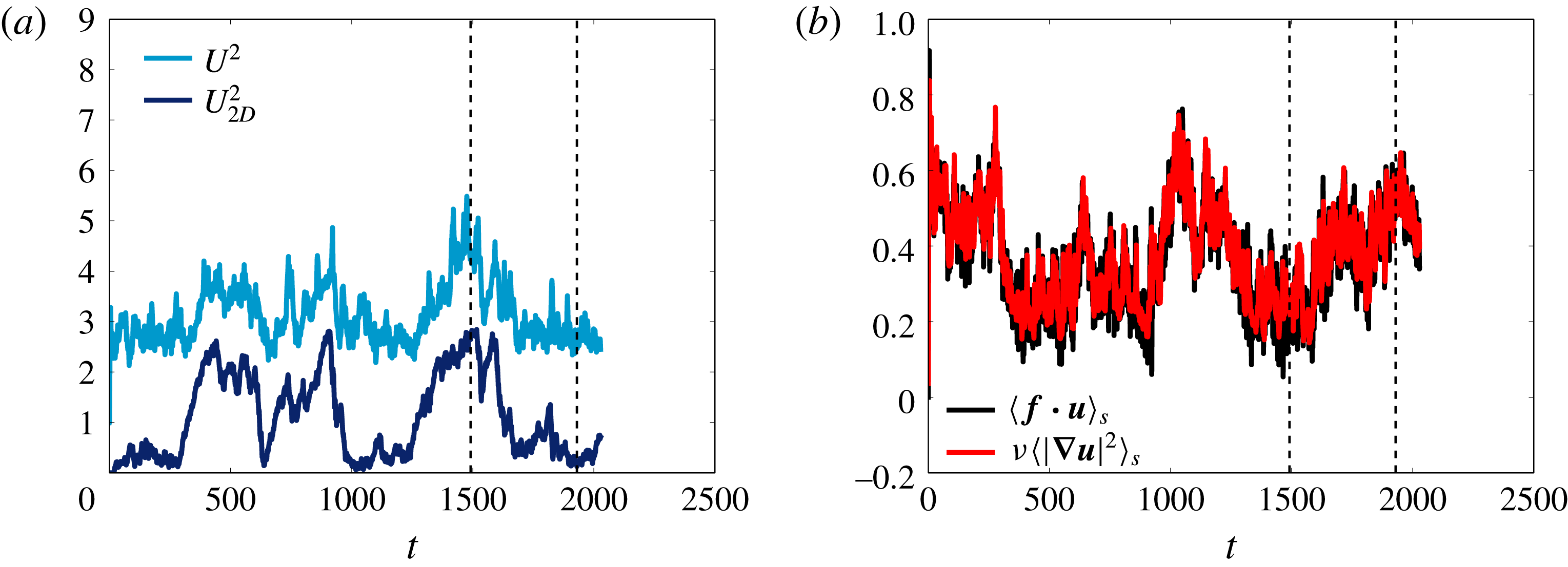
(a) Time series of the total energy
 $U^{2}$
and the energy at the large scales
 $U_{2D}^{2}$
for the case of
 $Ro_{f}=0.556,Re_{f}=100$
, which is close to
 $Ro_{f}^{\ast }$
. The vertical dashed lines denote the time instances at which the visualizations shown in figure 15 are taken. (b) Shows the spatial averaged energy injection rate
 $\langle \boldsymbol{f}\boldsymbol{\cdot }\boldsymbol{u}\rangle _{S}$
and the dissipation rate
 $\unicode[STIX]{x1D708}\langle |\unicode[STIX]{x1D735}\boldsymbol{u}|^{2}\rangle _{S}$
for the same run.

To understand this discrepancy, in figure 14(a) we show the time evolution of the total energy
 $U^{2}$
(lighter shade) and the energy of the large scales
 $U_{2D}^{2}$
for a value of
 $Ro_{f}=0.556$
close to the critical value and a relatively large
 $Re_{f}=100$
. The flow randomly oscillates between two distinct states: one where the energy of the large scales is weak and most of the energy lies in the forcing scales, and one where the energy of the large scales dominates and accounts for more than 60 % of the total energy. The energy at the large scales varies by an order of magnitude between these two states with
 $U_{2D}^{2}\sim \unicode[STIX]{x1D6FA}^{2}L^{2}$
when
 $U_{2D}^{2}$
dominates and
 $U_{2D}^{2}\ll \unicode[STIX]{x1D6FA}^{2}L^{2}$
at its low values. In figure 14(b) the time series of the spatial-averaged energy injection rate
 $\langle \boldsymbol{f}\boldsymbol{\cdot }\boldsymbol{u}\rangle _{S}$
and the energy dissipation rate
 $\unicode[STIX]{x1D708}\langle |\unicode[STIX]{x1D735}\boldsymbol{u}|^{2}\rangle _{S}$
is shown. A burst of energy dissipation is observed at the time instances that the flow transitions from the condensate to the 3D turbulent state. This correlation between the change of state in the large scales and the energy dissipation/injection is typical of bimodal systems (Mishra et al.
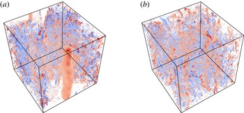
Reference Mishra, Herault, Fauve and Verma2015). Visualizations of the vertical vorticity of the flow are shown in figure 15 at the two different times indicated by the vertical dashed lines in figure 14(a,b). The two figures resemble the ones shown in figure 11(b,c) that were obtained for different values of the parameter
 $Ro_{f}$
.
It appears thus that the transition from isotropic turbulence to rotating condensate occurs through a bistable regime where both states are realized at different instances of time. The two states are distinct, i.e. they are separated by a finite amount of energy; however, the time the system spends in each one of these states can depend on the deviation from the onset
 $Ro_{f}^{\ast }$
, becoming infinite for the condensate state for
 $Ro_{f}$
sufficiently smaller than
 $Ro_{f}^{\ast }$
. The time-averaged quantities displayed in the previous sections thus remain continuous. This bistable behaviour, if it persists at larger
 $Re_{f}$
, will indicate that the transition will remain supercritical. Similar behaviour has been observed in experiments in a rotating tank where intermittent switching between blocked and large-scale zonal patterns has been observed Weeks et al. (Reference Weeks, Tian, Urbach, Ide, Swinney and Ghil1997). This presents an alternate mechanism other than the subcritical transition discussed in § 3 and observed in Alexakis (Reference Alexakis2015), Yokoyama & Takaoka (Reference Yokoyama and Takaoka2017).
The figures show the contours of the vertical vorticity
 $\unicode[STIX]{x1D714}_{z}$
for
 $Ro_{f}=0.556,Re_{f}=100$
for the two time instances marked in figure 14(a). Red colours correspond to positive vorticity and blue colours correspond to negative vorticity. In panel (a) a co-rotating vortex is formed when the system is in the condensate regime, while panel (b) does not have any large-scale structure.

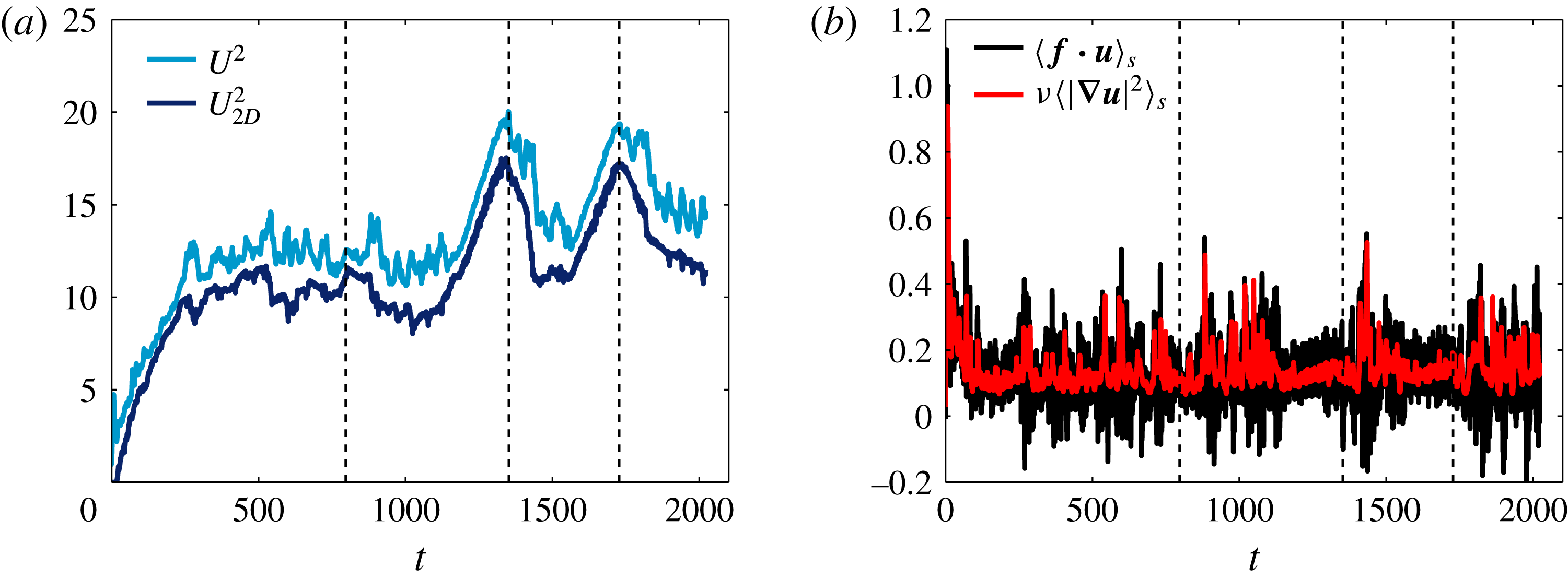
(a) The time series of the total energy
 $U^{2}$
and the energy at the large scales
 $U_{2D}^{2}$
for the case of
 $Ro_{f}=0.357,Re_{f}=100$
, which is below
 $Ro_{f}^{\ast }$
. The vertical dashed lines denote the time instances at which the visualizations shown in figure 17 are taken. (b) The spatial averaged energy injection rate
 $\langle \boldsymbol{f}\boldsymbol{\cdot }\boldsymbol{u}\rangle _{S}$
and the dissipation rate
 $\unicode[STIX]{x1D708}\langle |\unicode[STIX]{x1D735}\boldsymbol{u}|^{2}\rangle _{S}$
for the same run.

The figures show the contours of the vertical vorticity
 $\unicode[STIX]{x1D714}_{z}$
for
 $Ro_{f}=0.357,Re_{f}=100$
for the three time instances marked in figure 16(a). Red colours correspond to positive vorticity and blue colours correspond to negative vorticity.

A similar oscillating behaviour is observed even further from the onset
 $Ro_{f}^{\ast }$
. In figure 16(a) we show the time evolution of
 $U_{2D}^{2}$
and
 $U^{2}$
, as in figure 14(a), for a slightly smaller value of
 $Ro_{f}=0.357$
. Unlike the previous case the system here is only in the condensate regime with the energy concentrated at the largest scale
 $k\,L=1$
.
 $U_{2D}^{2}$
is always dominant and it undergoes strong fluctuations. Figure 16(b) shows the time series of the spatially averaged energy injection rate
 $\langle \boldsymbol{f}\boldsymbol{\cdot }\boldsymbol{u}\rangle _{S}$
and the energy dissipation rate
 $\unicode[STIX]{x1D708}\langle |\unicode[STIX]{x1D735}\boldsymbol{u}|^{2}\rangle _{S}$
for the same run as figure 16(a). The peaks of energy injection/dissipation are correlated with changes in the large-scale flow states. We note that in the condensate regime, even though the dissipation is always positive, the energy injection rate takes both negative and positive values. This means that at certain instances of time the forcing takes energy out of the system. Visualization of the flows in figure 17 at different times reveal that these fluctuations correspond to a transition of the flow from a state that has a co-rotating vortex that is stable to states that are unstable to 3D fluctuations that, however, fail to destroy it. Thus, it seems that the key to understanding the behaviour of this flow lies in understanding the stability properties of these freely evolving vortices.
6 Effect of helicity
Finally we comment on the effect of helicity on the condensate formation. Contrary to the small-scale behaviour, where the presence of helicity was shown to play a significant role (Mininni & Pouquet Reference Mininni and Pouquet2010; Sen et al. Reference Sen, Mininni, Rosenberg and Pouquet2012), in the present investigation it was shown that it did not affect the dynamics of the observed large-scale quantities. Both helical and non-helical flows were shown to obey the same scaling laws, and only small variations were observed in the prefactors. This is perhaps not surprising since helicity cascades to the small scales, and thus it does not affect the large scales of the condensates.
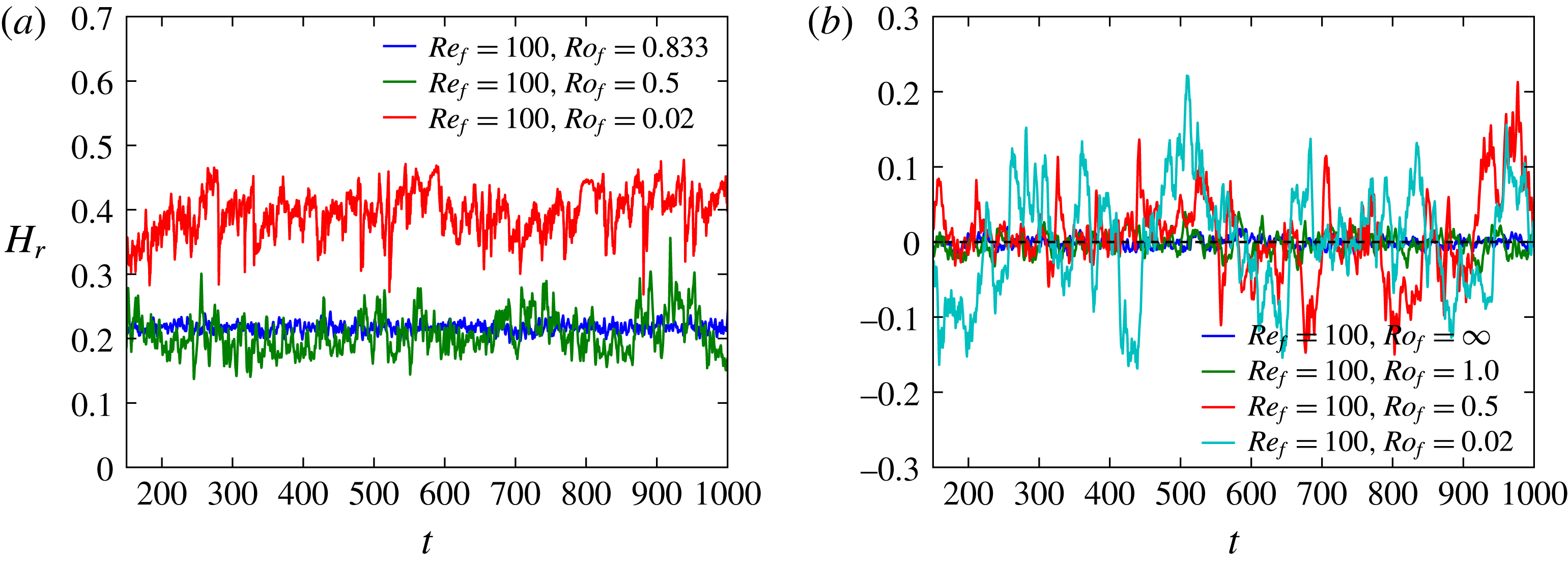
The figures show the time series of the relative helicity
 $H_{r}$
as a function of time for a few different Rossby numbers and fixed
 $Re_{f}=100.0$
for (a) helical runs and (b) non-helical runs.

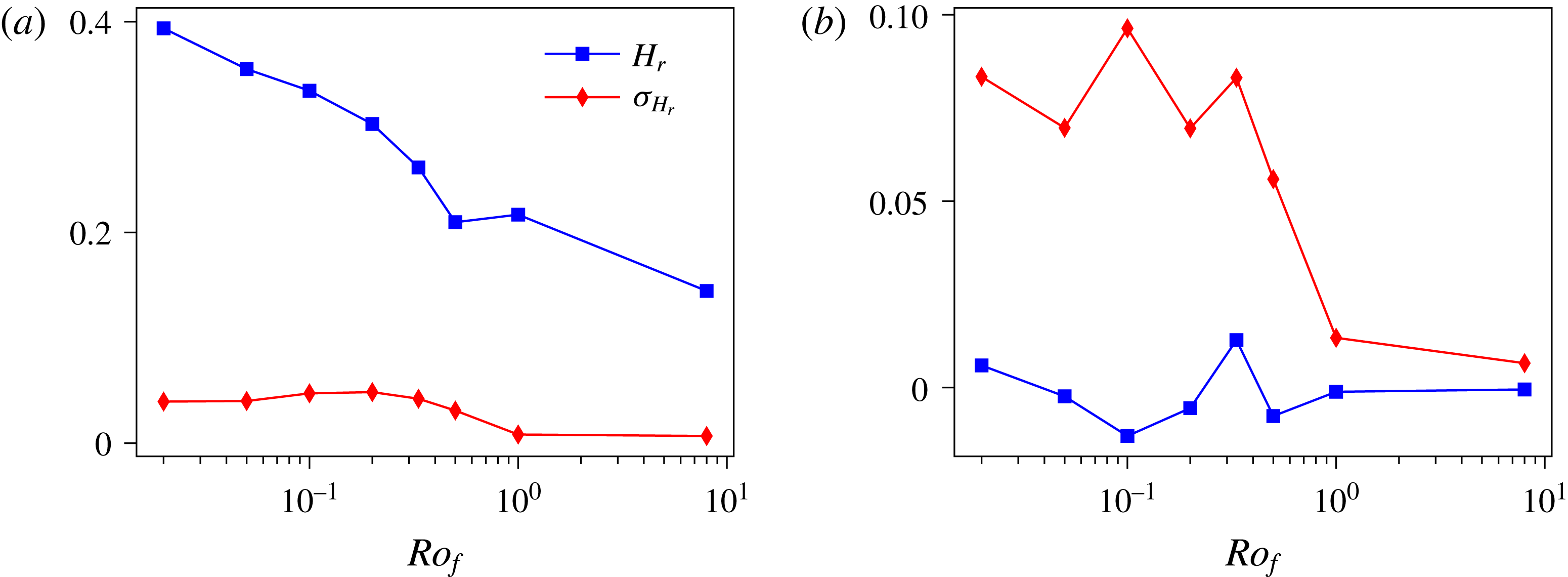
The figures show the relative helicity
 $H_{r}$
and the standard deviation of the relative helicity
 $\unicode[STIX]{x1D70E}_{H_{r}}$
as a function of
 $Ro_{f}$
for fixed
 $Re_{f}=100$
for (a) helical runs and (b) non-helical runs.

In figure 18 we show the time series of the relative helicity
 $H_{r}$
for a few different values of
 $Ro_{f}$
and fixed
 $Re_{f}=100$
for both the helical and the non-helical cases. The relative helicity is defined as
 $$\begin{eqnarray}H_{r}=\frac{\langle \boldsymbol{u}\boldsymbol{\cdot }\unicode[STIX]{x1D735}\times \boldsymbol{u}\rangle _{S}}{\langle |\boldsymbol{u}|^{2}\rangle _{S}^{1/2}\langle |\unicode[STIX]{x1D735}\times \boldsymbol{u}|^{2}\rangle _{S}^{1/2}}.\end{eqnarray}$$
For the helical forcing case the relative helicity is always non-zero and increases as we reduce
 $Ro_{f}$
. For the small values of
 $Ro_{f}$
it reaches a value of approximately
 $0.4$
. For the non-helical case the relative helicity oscillates around zero; however, with the fluctuations being significantly strong and larger for smaller values of
 $Ro_{f}$
. It is also worth noting that the time scale of these fluctuations increases as the rotation becomes larger. This has already been observed in Dallas & Tobias (Reference Dallas and Tobias2016).
In figure 19 we show the time-averaged relative helicity
 $H_{r}$
and the standard deviation of the relation helicity
 $\unicode[STIX]{x1D70E}_{H_{r}}$
as a function of
 $Ro_{f}$
for both helical and non-helical forcing with
 $Re_{f}=100$
. For the helical forcing, as
 $Ro_{f}$
is decreased the relative helicity and the fluctuations increase. For the non-helical case, also the fluctuations increase when
 $Ro_{f}$
is decreased below the critical value, even if the mean remains zero. The fluctuations in the mean helicity can play an important role for dynamo studies in turbulent rotating flows (see Seshasayanan, Dallas & Alexakis Reference Seshasayanan, Dallas and Alexakis2017).
7 Conclusions
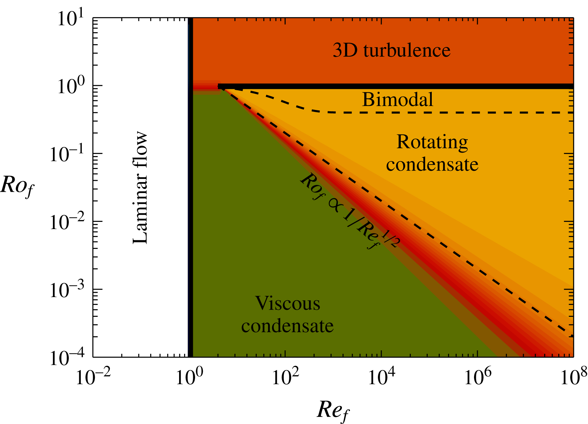
This work gives a description of steady-state rotating turbulence when the forcing acts directly on the slow manifold, by mapping the parameter space with the different behaviours observed and the resulting scaling relations. Our results are concisely summarized in figure 20, where the four different phases of the rotating flows examined are shown in the parameter space (
 $Re_{f},Ro_{f}$
): laminar flow, 3D turbulence flow, rotating condensate flow and viscous condensate flow. Solid lines indicate the boundaries where a critical transition takes place, while dashed lines indicate smooth transitions.
The figure shows the phase space diagram with the different flow behaviour marked. Solid lines denote sharp/critical transitions. Dashed line denotes smooth transitions.

For values of
 $Re_{f}$
below a critical value
 $Re_{f}^{\ast }$
that is independent of
 $Ro_{f}$
, the flow has a laminar behaviour. At this state the resulting flow is 2D, independent of time, and proportional to the inverse Laplacian of the forcing. The first unstable mode in this laminar state is a 2D mode that is not affected by the rotation, and thus the instability boundary does not depend on
 $Ro_{f}$
.
For
 $Re_{f}\gg Re_{f}^{\ast }$
and
 $Ro_{f}$
above a critical value
 $Ro_{f}^{\ast }$
, the flow displays quasi-isotropic 3D turbulence. This regime is described to a good degree by Kolmogorov–Richardson phenomenology (Richardson Reference Richardson1926; Kolmogorov Reference Kolmogorov1941), and classical results of turbulence like the finite energy dissipation at the zero-viscosity limit and a
 $k^{-5/3}$
energy spectrum appear to hold.
For
 $Re_{f}\gg Re_{f}^{\ast }$
and
 $Re_{f}^{-1/2}\ll Ro_{f}\leqslant Ro_{f}^{\ast }$
, the flow is shown to be in what we refer as a rotating condensate state. In this state a co-rotating 2D vortex is dominant at the large scales while the counter-rotating vortex breaks down to 3D eddies cascading energy back to the small scales. At this state the amplitude of the condensate
 $U_{2D}$
(in the rather small range examined by our simulations) was shown to be proportional to the rotation rate
 $U_{2D}\propto \unicode[STIX]{x1D6FA}L$
. Our results also indicate (with the help of hyperviscous simulations) that in this regime the finite energy dissipation at the zero-viscosity limit still holds but with a drag coefficient that rapidly decreases with
 $Ro_{f}$
. The spectra at the small scales follow a close to
 $k^{-5/3}$
power law, while a large peak appears at the largest scale, indicating the presence of the condensate.
The transition from the quasi-isotropic 3D turbulent state to the rotating condensate state was shown to be supercritical, contrary to the arguments described in the introduction that were predicting that at sufficiently large
 $Re_{f}$
, right below criticality
 $Ro_{f}^{\ast }$
, the system would transition discontinuously to the rotating condensate value
 $U_{2D}^{2}\propto \unicode[STIX]{x1D6FA}^{2}L^{2}$
. The reason for this discrepancy is in part because the arguments in § 3 assumed weak dependence of the energy injection rate
 $\unicode[STIX]{x1D716}$
at criticality, while the DNS showed a strong sensitivity of
 $\unicode[STIX]{x1D716}$
on
 $Ro_{f}$
close to criticality. The second reason is that the system close to criticality showed a bimodal behaviour where part of the time was spent in the 3D turbulence state with
 $U_{2D}^{2}\ll \unicode[STIX]{x1D6FA}^{2}L^{2}$
and the remaining part was spent in the rotating condensate state with
 $U_{2D}^{2}\propto \unicode[STIX]{x1D6FA}^{2}L^{2}$
. Despite the fact that these states have distinct energy levels, the time spent in the condensate state can decrease continuously to zero as
 $Ro_{f}\rightarrow Ro_{f}^{\ast }$
(from below), leading to a continuous supercritical transition.
For
 $Re_{f}\gg Re_{f}^{\ast }$
and
 $Ro_{f}\ll Re_{f}^{-1/2}$
the flow is shown to be in what we refer to as a viscous condensate state. In this state the flow is close to 2D and both the co-rotating and counter-rotating 2D vortices exist and dominate the large scales. The flow has a normalized energy dissipation rate that decreases with
 $Re_{u}$
, following the laminar scaling
 $Re_{u}^{-1}$
. The transition from the rotating condensate regime to the viscous condensate was found to be smooth. We note, however, that another critical value of
 $Ro_{f}$
is expected for which the flow becomes exactly 2D and all 3D perturbations decay exponentially (Gallet Reference Gallet2015). Such a transition is expected at even smaller values of
 $Ro_{f}$
, and to observe it we have to focus on deviations from 2D flows, which was not done in the present study. A similar study in thin layers has shown that this transition is governed by strong intermittent events (Benavides & Alexakis Reference Benavides and Alexakis2017). Thus, this is an interesting limit that is worth investigating in the future.
The difference between the parameters
 $(Re_{f},Ro_{f})$
and
 $(Re_{u},Ro_{u})$
or
 $(Re_{\unicode[STIX]{x1D716}},Ro_{\unicode[STIX]{x1D716}})$
was not found to be as severe as in the Taylor–Green flow, where discontinuous (subcritical) transitions were present, which results in mapping from one set of parameters to the other being neither one-to-one nor onto. In particular, the difference between
 $(Re_{f},Ro_{f})$
and
 $(Re_{\unicode[STIX]{x1D716}},Ro_{\unicode[STIX]{x1D716}})$
was only found to be significant close to the critical point
 $Ro_{f}^{\ast }$
where
 $\unicode[STIX]{x1D716}$
was found to change abruptly. The difference between
 $(Re_{f},Ro_{f})$
and
 $(Re_{u},Ro_{u})$
was stronger, and is due to the fact that in the rotating condensate regime the scaling
 $U\propto \unicode[STIX]{x1D6FA}L$
merged all values of
 $Ro_{u}$
to be close to unity. This left all larger values of
 $Ro_{u}$
to be in the viscous condensate regime. Thus, in the steady-state regime, at least
 $Ro_{u}$
does not appear to be a good indicator for the strength of rotation.
We stress the importance of the ordering of the limits when one considers the low-Rossby-number, large-Reynolds-number limit. If one considers the
 $Ro_{f}\rightarrow 0$
limit first, and afterwards the
 $Re_{f}\rightarrow \infty$
limit then one always falls in the viscous condensate regime. While if one considers the
 $Re_{f}\rightarrow \infty$
first one falls in the rotating condensate regime. To distinguish between the two one needs to look at the products
 $Ro_{f}Re_{f}^{1/2}$
or
 $Ro_{\unicode[STIX]{x1D706}}=Ro_{\unicode[STIX]{x1D716}}Re_{\unicode[STIX]{x1D716}}^{1/2}$
. Referring thus to the large-Reynolds-number, small-Rossby-number limit is ambiguous unless the ordering is specified.
The presence or absence of helicity in the forcing does not affect the dynamics of the large-scale condensates. Both helical and non-helical forcing lead to similar bifurcation diagrams and scaling laws for the large-scale quantities. This perhaps could have been expected since helicity is a quantity that cascades to the small scales and is unlikely to affect the condensate scales. However, the normalized mean helicity did display non-trivial dynamics. Its mean value increased as
 $Ro_{f}$
was decreased for the helical forcing case, while for the non-helical forcing even if the mean value was zero then strong fluctuations were present. In both cases the fluctuations of the relative helicity are stronger in the condensate regime.
We note that the results presented here are obtained in a cubic box. Varying box height gives rise to different values of
 $Ro_{f}^{\ast }$
, as discussed in § 3 (see Deusebio et al.
Reference Deusebio, Boffetta, Lindborg and Musacchio2014). Also varying the box size in the horizontal direction with respect to the forcing length scale is something that has not been examined in our runs. Although we have concluded the scaling
 $U_{2D}^{2}\sim \unicode[STIX]{x1D6FA}^{2}L^{2}$
for the amplitude of the condensate, we have only verified this scaling with rotation and not with the box size
 $L$
. This is something that needs to be examined in future investigations. Furthermore, the presence of anisotropy in the two horizontal directions tends to alter the structure of the flow from vortex dipoles to shear layers, as has been suggested in Bouchet & Simonnet (Reference Bouchet and Simonnet2009), Bouchet & Venaille (Reference Bouchet and Venaille2012) and shown recently for 2D turbulence (Frishman, Laurie & Falkovich Reference Frishman, Laurie and Falkovich2017), and rapidly rotating convection (Guervilly & Hughes Reference Guervilly and Hughes2017; Julien, Knobloch & Plumley Reference Julien, Knobloch and Plumley2018) and this is a new direction where condensate dynamics could be studied.
Finally, we comment on the effect of boundaries and the realizability of the present results in experiments. In the present results we considered only the simplest domain, that of a triple periodic geometry, and we should give a word of caution in extrapolating them to domains with no-slip boundary conditions. In the presence of no-slip boundaries, rotation will introduce Ekman layers (Ekman Reference Ekman1905) that can lead to large-scale drag effects (Caldwell, Van Atta & Helland Reference Caldwell, Van Atta and Helland1972; Howroyd & Slawson Reference Howroyd and Slawson1975; Zavala Sansón, van Heijst & Backx Reference Zavala Sansón, van Heijst and Backx2001; Sous, Sommeria & Boyer Reference Sous, Sommeria and Boyer2013), altering in part the energy balance. Nonetheless, we do believe that in a carefully prepared experimental set-up where these effects are accounted for some of the presently observed phenomena would carry over to no-slip boundary conditions. In particular, it would be interesting to investigate the transition to the rotating condensate regime from 3D turbulence that displayed such rich behaviour. The high numerical cost of 3D simulations in this regime limits our runs to relatively short times, and does not allow us to study in detail their statistical behaviour. Experiments where long time series are easily attainable can then address this issue.
Acknowledgements
The authors would like to acknowledge various discussions with S. Fauve and the nonlinear physics group at ENS. This work was granted access to the HPC resources of MesoPSL financed by the Region Ile de France and the project Equip@Meso (reference ANR-10-EQPX-29-01) of the program Investissements d’Avenir, supervised by the Agence Nationale pour la Recherche, and the HPC resources of GENCI-TGCC-CURIE and GENCI-CINES-OCCIGEN (Project nos. x2015056421, x2016056421 and A0010506421) where the present numerical simulations have been performed.