1 Introduction
One of the classic issues in aerodynamics is the estimation of the lift response of a wing in unsteady flow. Based on unsteady thin-airfoil theory, Sears (Reference Sears1938) derived the lift formula for a two-dimensional wing in a sinusoidal vertical gust. In Sears’ analysis, the velocity fluctuation is simplified by having a constant spanwise spatial distribution and is variable in the streamwise direction only. The transfer function, which characterizes the interaction of the incident velocity fluctuation with the strip of the wing, is consequently only a function of the streamwise wavenumber (the one-wavenumber transfer function). However, the measured unsteady lift of a wing in turbulent flow is usually lower than Sears’ theoretical values (Lamson Reference Lamson1957; Jackson, Graham & Maull Reference Jackson, Graham and Maull1973). This phenomenon is also confirmed in the measurement concerning other streamlined structures (Larose & Mann Reference Larose and Mann1998; Larose Reference Larose1999; Ma Reference Ma2007). It is known that turbulence is a three-dimensional flow field and can be regarded as the superposition of yawed sinusoidal gust components. The velocity fluctuation is therefore variable both in the streamwise and spanwise directions. This brings in a new variable, the spanwise wavenumber. In this case, the interaction of the velocity fluctuation with the strip of the wing depends not only on the local velocity fluctuation but also on the velocity fluctuation at other spanwise positions. Hence, besides the velocity fluctuation, the transfer function is also a function of the streamwise and spanwise wavenumbers (the two-wavenumber transfer function). The exact values of the two-wavenumber transfer function were calculated numerically by Graham (Reference Graham1970, Reference Graham1971). Other aerodynamicists (Filotas Reference Filotas1969; Mugridge Reference Mugridge1971; Blake Reference Blake1986) derived approximate closed-form expressions for the Graham’s two-wavenumber transfer function.
Because both the incident velocity fluctuation and the transfer function are influenced by the spanwise wavenumber, the measured unsteady lift of a wing in turbulent flow does not agree with Sears’ theoretical predictions. In general, the two-wavenumber analysis is needed to account for the influence of the spanwise wavenumber in this case (Li, Li & Liao Reference Li, Li and Liao2015; Li & Li Reference Li and Li2017). To simplify the problem, here we invoke the strip assumption. Under this assumption, the interaction of the incident velocity fluctuation with the strip of the wing is still regarded to be two-dimensional, despite the fact that the velocity fluctuation contains the spanwise wavenumber. In other words, the influence of the spanwise wavenumber on the transfer function can be considered to be negligible, and the two-wavenumber transfer function can be replaced by the one-wavenumber transfer function. The strip assumption is of interest in practical applications because the use of the one-wavenumber transfer function instead of the two-wavenumber transfer function simplifies significantly the related calculations. For a flat plate cross-section, the one-wavenumber transfer function is the well-known Sears function. It should be noted that, for a non-flat plate cross-section, the Sears function still lacks a systematic verification in terms of frequency dependence (Cordes et al. Reference Cordes, Kampers, Meißner, Tropea, Peinke and Hölling2017). It is known that the Sears function is derived based on the flat plate assumption. This may be a reasonable assumption at low frequencies, however, at high frequencies, where the relevant turbulent length scales are comparable to the thickness, the flat plate assumption is invalid and leads to overestimation of the lift (Glegg & Devenport Reference Glegg and Devenport2009; Devenport, Staubs & Glegg Reference Devenport, Staubs and Glegg2010; Lysak, Capone & Jonson Reference Lysak, Capone and Jonson2013, Reference Lysak, Capone and Jonson2016). When using the Sears function to calculate the unsteady lift of an actual wing in turbulent flow, it is necessary to verify its applicability.
The aim of this work is to investigate to what extent the strip assumption can be used to estimate the unsteady lift response of a two-dimensional wing in turbulent flow. For this purpose, we first need to know the parameters that control the accuracy of the strip assumption. Although some theoretical studies (Filotas Reference Filotas1971; Massaro & Graham Reference Massaro and Graham2015) have indicated that the aspect ratio has an effect on the accuracy of the strip assumption, the related experimental investigation combining the turbulence characteristics is still missing. In this paper, we show that the accuracy of the strip assumption is controlled by the ratio of the turbulence integral scale to the chord and the aspect ratio. By increasing these two parameters, the accuracy of the strip assumption is improved, and the one-wavenumber transfer function obtained from the strip assumption is close to the Sears function. Then, for wings with three different aspect ratios, we compare the experimental one-wavenumber transfer functions obtained from the strip assumption with the theoretical predictions. Finally, we discuss the effect of the thickness on the transfer function.
2 Theoretical analysis
The present theoretical analysis is concerned with the case of a wing in turbulent flow. The following assumptions regarding the wing and the turbulent flow are made: (i) the cross-section of the wing is an idealized thin airfoil without thickness, camber and angle of attack so that the Sears function and the Graham’s two-wavenumber transfer function can be used; (ii) the turbulent flow is homogeneous and isotropic, in fact, to simplify the problem, the statistics of the turbulent fluctuations are often arranged to be spatially homogeneous and isotropic (Davidson Reference Davidson2004); (iii) the wing is a two-dimensional (infinite) wing without tips. Note that the aspect ratio of the wing was previously used to refer to the ratio of its whole span to its chord. Here, the wing involved is infinite, and the aspect ratio has another meaning: it refers to the ratio of the specified span (a finite specified spanwise length of the infinite wing) to the chord. The unsteady lift is calculated over this specified finite spanwise length, and this length can be taken anywhere along the span due to the assumed homogeneity of the turbulent flow.
2.1 Comparison between the two-wavenumber analysis and the strip assumption
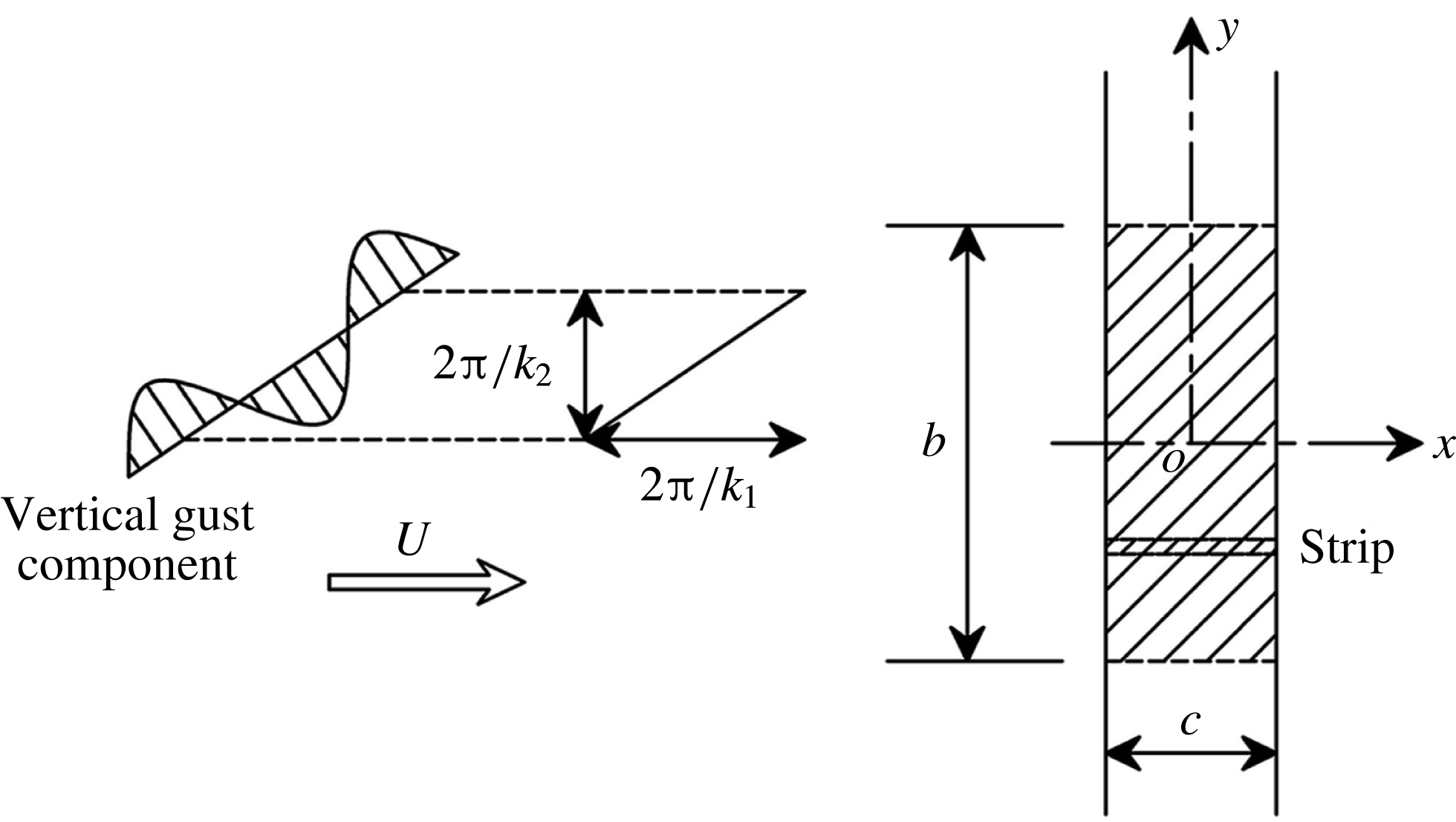
The wing of a thin-airfoil cross-section may be sensitive only to the flow field in its own plane. The three-dimensional turbulent flow can be thus simplified as the superposition of yawed sinusoidal vertical gust components in a two-dimensional plane. Figure 1 is the coordinate system used in the analysis and shows an infinite wing in a yawed sinusoidal vertical gust with variation in the streamwise and spanwise directions. The special case with spanwise wavenumber
 $k_{2}=0$
is the well-known one-dimensional sinusoidal vertical gust problem of Sears (Reference Sears1938). In this case, the vertical velocity fluctuation has a constant spanwise spatial distribution. Taking the origin for x at the centre of the wing, the upwash velocity is written as
 $w=w_{0}\text{e}^{\text{i}\unicode[STIX]{x1D708}(x/U-t)}$
. The unsteady lift on the strip is
 $$\begin{eqnarray}\displaystyle & \displaystyle L_{2d}=\unicode[STIX]{x03C0}\unicode[STIX]{x1D70C}Ucw_{0}\text{e}^{-\text{i}\unicode[STIX]{x1D708}t}S\left({\displaystyle \frac{k_{1}c}{2}}\right), & \displaystyle\end{eqnarray}$$
where
 $\unicode[STIX]{x1D70C}$
is the fluid density,
 $U$
is the mean flow velocity,
 $c$
is the chord,
 $w_{0}$
is the gust amplitude,
 $\unicode[STIX]{x1D708}=2\unicode[STIX]{x03C0}f$
is the circular frequency,
 $f$
is the gust frequency,
 $k_{1}=\unicode[STIX]{x1D708}/U$
is the streamwise wavenumber,
 $S(k_{1}c/2)$
is the Sears function. Using (2.1) and neglecting the spanwise variation of the turbulent flow, Liepmann (Reference Liepmann1952) gave the one-wavenumber lift spectrum on the strip of a wing in turbulent flow, which is
 $$\begin{eqnarray}\displaystyle & \displaystyle \unicode[STIX]{x1D719}_{L2d}(k_{1})=(\unicode[STIX]{x03C0}\unicode[STIX]{x1D70C}Uc)^{2}\left|S\left({\displaystyle \frac{k_{1}c}{2}}\right)\right|^{2}\unicode[STIX]{x1D719}_{w}(k_{1}), & \displaystyle\end{eqnarray}$$
where
 $\unicode[STIX]{x1D719}_{w}(k_{1})$
is the one-wavenumber spectrum of the vertical velocity fluctuation.
 $|\cdot |^{2}$
is the symbol for the square of the module.
The coordinate system of an infinite wing in a yawed sinusoidal vertical gust component with streamwise and spanwise variations.

For the more general case which the spanwise wavenumber
 $k_{2}$
is not zero, or say, the vertical velocity fluctuation is not fully correlated in the spanwise direction, the upwash velocity has the form
 $w=w_{0}\text{e}^{\text{i}[\unicode[STIX]{x1D708}(x/U-t)+k_{2}y]}$
. The unsteady lift on the strip was obtained by Graham (Reference Graham1970, Reference Graham1971). It is
 $$\begin{eqnarray}\displaystyle & \displaystyle L_{3d}=\unicode[STIX]{x03C0}\unicode[STIX]{x1D70C}Ucw_{0}\text{e}^{\text{i}(k_{2}y-\unicode[STIX]{x1D708}t)}G\left({\displaystyle \frac{k_{1}c}{2}},{\displaystyle \frac{k_{2}c}{2}}\right), & \displaystyle\end{eqnarray}$$
where
 $G(k_{1}c/2,k_{2}c/2)$
is Graham’s two-wavenumber transfer function. The total unsteady lift for a span extending from
 $y=-b/2$
to
 $b/2$
can be obtained by integrating equation (2.3). Then the unsteady lift per unit span of this spanwise integral region (the shaded region of the wing shown in figure 1) is
 $$\begin{eqnarray}\displaystyle \displaystyle L_{3dm} & = & \displaystyle {\displaystyle \frac{1}{b}}\int _{-b/2}^{b/2}\unicode[STIX]{x03C0}\unicode[STIX]{x1D70C}Ucw_{0}\text{e}^{\text{i}(k_{2}y-\unicode[STIX]{x1D708}t)}G\left({\displaystyle \frac{k_{1}c}{2}},{\displaystyle \frac{k_{2}c}{2}}\right)\text{d}y\nonumber\\ \displaystyle & = & \displaystyle \unicode[STIX]{x03C0}\unicode[STIX]{x1D70C}Ucw_{0}\text{e}^{-\text{i}\unicode[STIX]{x1D708}t}\text{sinc}\left({\displaystyle \frac{k_{2}b}{2}}\right)G\left({\displaystyle \frac{k_{1}c}{2}},{\displaystyle \frac{k_{2}c}{2}}\right),\end{eqnarray}$$
where
 $b$
is the span,
 $\text{sinc}$
is the sinc function. Note that (2.4) is the gust response to a single yaw gust. Using the generalized spectral approach of Ribner (Reference Ribner1956) and (2.4), Jackson et al. (Reference Jackson, Graham and Maull1973) showed that the one-wavenumber lift spectrum per unit span of the spanwise region for a wing in turbulent flow could be written as
 $$\begin{eqnarray}\displaystyle & \displaystyle \unicode[STIX]{x1D719}_{L3dm}(k_{1})=(\unicode[STIX]{x03C0}\unicode[STIX]{x1D70C}Uc)^{2}\int _{-\infty }^{\infty }\text{sinc}^{2}\left({\displaystyle \frac{k_{2}b}{2}}\right)\left|G\left({\displaystyle \frac{k_{1}c}{2}},{\displaystyle \frac{k_{2}c}{2}}\right)\right|^{2}\unicode[STIX]{x1D6F7}_{w}(k_{1},k_{2})\,\text{d}k_{2}, & \displaystyle\end{eqnarray}$$
where
 $\unicode[STIX]{x1D6F7}_{w}(k_{1},k_{2})$
is the two-wavenumber spectrum of the vertical velocity fluctuation.
Now we invoke the strip assumption. Under this assumption, the transfer function of the unsteady lift on the strip of the spanwise region is still regarded to be a function of the streamwise wavenumber only.
 $G(k_{1}c/2,k_{2}c/2)$
can be thus replaced by
 $S(k_{1}c/2)$
. The form of upwash velocity does not change in this case, equation (2.5) then becomes
 $$\begin{eqnarray}\displaystyle & \displaystyle \unicode[STIX]{x1D719}_{L3dms}(k_{1})=(\unicode[STIX]{x03C0}\unicode[STIX]{x1D70C}Uc)^{2}\int _{-\infty }^{\infty }\text{sinc}^{2}\left({\displaystyle \frac{k_{2}b}{2}}\right)\left|S\left({\displaystyle \frac{k_{1}c}{2}}\right)\right|^{2}\unicode[STIX]{x1D6F7}_{w}(k_{1},k_{2})\,\text{d}k_{2}. & \displaystyle\end{eqnarray}$$
Based on the equivalence principle of force, the ratio
 $\unicode[STIX]{x1D713}$
evaluating the accuracy of strip assumption can be obtained by comparing the one-wavenumber lift spectrum
 $\unicode[STIX]{x1D6F7}_{L3dm}(k_{1})$
calculated from (2.5) with the lift spectrum
 $\unicode[STIX]{x1D6F7}_{L3dms}(k_{1})$
calculated from (2.6). That is
 $$\begin{eqnarray}\displaystyle & \displaystyle \unicode[STIX]{x1D713}={\displaystyle \frac{\unicode[STIX]{x1D719}_{L3dm}(k_{1})}{\unicode[STIX]{x1D719}_{L3dms}(k_{1})}}={\displaystyle \frac{\displaystyle \int _{-\infty }^{\infty }\text{sinc}^{2}\left({\displaystyle \frac{k_{2}b}{2}}\right)\left|G\left({\displaystyle \frac{k_{1}c}{2}},{\displaystyle \frac{k_{2}c}{2}}\right)\right|^{2}\unicode[STIX]{x1D6F7}_{w}(k_{1},k_{2})\,\text{d}k_{2}}{\displaystyle \int _{-\infty }^{\infty }\text{sinc}^{2}\left({\displaystyle \frac{k_{2}b}{2}}\right)\left|S\left({\displaystyle \frac{k_{1}c}{2}}\right)\right|^{2}\unicode[STIX]{x1D6F7}_{w}(k_{1},k_{2})\,\text{d}k_{2}}}. & \displaystyle\end{eqnarray}$$
For comparison purposes, we introduce the approximate closed-form expression of Graham’s two-wavenumber transfer function derived by Blake (Reference Blake1986). Blake’s approximation is in terms of a two-wavenumber influence factor
 $\unicode[STIX]{x1D702}(k_{1}c,k_{2}c)$
to the Sears function, which is expressed as
 $$\begin{eqnarray}\displaystyle & \displaystyle \left|G\left({\displaystyle \frac{k_{1}c}{2}},{\displaystyle \frac{k_{2}c}{2}}\right)\right|^{2}=\left|S\left({\displaystyle \frac{k_{1}c}{2}}\right)\right|^{2}\unicode[STIX]{x1D702}(k_{1}c,k_{2}c), & \displaystyle\end{eqnarray}$$
 $$\begin{eqnarray}\displaystyle & \displaystyle \unicode[STIX]{x1D702}(k_{1}c,k_{2}c)={\displaystyle \frac{1+3.2(k_{1}c)^{1/2}}{1+3.2(k_{1}c)^{1/2}+2.4(k_{2}c)^{2}}}. & \displaystyle\end{eqnarray}$$
Calculation of
 $\unicode[STIX]{x1D713}$
also requires information regarding the two-wavenumber turbulence spectrum of the vertical velocity fluctuation,
 $\unicode[STIX]{x1D6F7}_{w}(k_{1},k_{2})$
. For homogeneous and isotropic turbulence, a general two-wavenumber turbulence spectral model can be introduced. It is (Li et al.
Reference Li, Li and Liao2015)
 $$\begin{eqnarray}\displaystyle & \displaystyle \unicode[STIX]{x1D6F7}_{w}(k_{1},k_{2})={\displaystyle \frac{8\unicode[STIX]{x03C0}\unicode[STIX]{x1D70E}_{w}^{2}a^{4}n(n+1)(k_{1}^{2}+k_{2}^{2})}{[1+a^{2}(k_{1}^{2}+k_{2}^{2})]^{n+2}}}, & \displaystyle\end{eqnarray}$$
 $$\begin{eqnarray}\displaystyle & \displaystyle a=L_{u}^{x}[\sqrt{\unicode[STIX]{x03C0}}\unicode[STIX]{x1D6E4}(n+1/2)/\unicode[STIX]{x1D6E4}(n)]^{-1}. & \displaystyle\end{eqnarray}$$
 $n$
and
 $a$
are parameters governing the shape and scale of the turbulence spectrum respectively.
 $L_{u}^{x}$
is the longitudinal integral scale,
 $\unicode[STIX]{x1D6E4}(n)$
is the gamma function,
 $\unicode[STIX]{x1D70E}_{w}^{2}$
is the mean square of the vertical velocity fluctuation. In general, the spectrum of homogeneous and isotropic turbulence (e.g. grid-generated turbulence) agrees with the von Kármán model (Roberts & Surry Reference Roberts and Surry1973; Nagata et al.
Reference Nagata, Hunt, Sakai and Wong2011), thus
 $n=1/3$
, and
 $a\approx 1.339L_{u}^{x}$
. For isotropic turbulence, there is an isotropic relationship
 $L_{u}^{x}=2L_{w}^{x}$
(Kitamura et al.
Reference Kitamura, Nagata, Sakai and Harasaki2014),
 $L_{w}^{x}$
is the vertical integral scale. Thus
 $a\approx 2.678L_{w}^{x}$
.
The presentation of
 $\unicode[STIX]{x1D713}$
is best given in terms of dimensionless parameters: the reduced frequency
 $\tilde{k}_{1}=k_{1}c/2$
,
 $\tilde{k}_{2}=k_{2}c/2$
, the aspect ratio
 $\unicode[STIX]{x1D703}=b/c$
and the ratio of the vertical integral scale to the chord
 $\unicode[STIX]{x1D6FE}=L_{w}^{x}/c$
. Combining equations (2.7), (2.8) and (2.9), the ratio
 $\unicode[STIX]{x1D713}$
is then written as follows
 $$\begin{eqnarray}\displaystyle & \displaystyle \unicode[STIX]{x1D713}\left({\displaystyle \frac{k_{1}c}{2}},\unicode[STIX]{x1D703},\unicode[STIX]{x1D6FE}\right)={\displaystyle \frac{\displaystyle \int _{-\infty }^{\infty }\text{sinc}^{2}(\tilde{k}_{2}\unicode[STIX]{x1D703})\unicode[STIX]{x1D702}(\tilde{k}_{1},\tilde{k}_{2})\unicode[STIX]{x1D709}(\tilde{k}_{1},\tilde{k}_{2},\unicode[STIX]{x1D6FE})\,\text{d}\tilde{k}_{2}}{\displaystyle \int _{-\infty }^{\infty }\text{sinc}^{2}(\tilde{k}_{2}\unicode[STIX]{x1D703})\unicode[STIX]{x1D709}(\tilde{k}_{1},\tilde{k}_{2},\unicode[STIX]{x1D6FE})\,\text{d}\tilde{k}_{2}}}, & \displaystyle\end{eqnarray}$$
 $$\begin{eqnarray}\displaystyle & \displaystyle \unicode[STIX]{x1D702}(\tilde{k}_{1},\tilde{k}_{2})={\displaystyle \frac{1+3.2(2\tilde{k}_{1})^{1/2}}{1+3.2(2\tilde{k}_{1})^{1/2}+2.4(2\tilde{k}_{2})^{2}}}, & \displaystyle\end{eqnarray}$$
 $$\begin{eqnarray}\displaystyle & \displaystyle \unicode[STIX]{x1D709}(\tilde{k}_{1},\tilde{k}_{2},\unicode[STIX]{x1D6FE})={\displaystyle \frac{\tilde{k}_{1}^{2}+\tilde{k}_{2}^{2}}{[1+(5.356\unicode[STIX]{x1D6FE})^{2}(\tilde{k}_{1}^{2}+\tilde{k}_{2}^{2})]^{7/3}}}. & \displaystyle\end{eqnarray}$$
The ratio
 $\unicode[STIX]{x1D713}$
as a function of the aspect ratio
 $\unicode[STIX]{x1D703}$
and the ratio of the vertical integral scale to the chord
 $\unicode[STIX]{x1D6FE}$
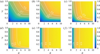
at different reduced frequencies is presented in figure 2. It can be seen that
 $\unicode[STIX]{x1D713}$
depends on
 $\unicode[STIX]{x1D703}$
and
 $\unicode[STIX]{x1D6FE}$
. The values of
 $\unicode[STIX]{x1D713}$
are between 0 and 1, and increase with increasing
 $\unicode[STIX]{x1D703}$
and
 $\unicode[STIX]{x1D6FE}$
. For the same group of
 $\unicode[STIX]{x1D703}$
and
 $\unicode[STIX]{x1D6FE}$
, the values of
 $\unicode[STIX]{x1D713}$
at high frequencies are larger than the values of
 $\unicode[STIX]{x1D713}$
at low frequencies. At low frequencies, the increase of the value of
 $\unicode[STIX]{x1D713}$
requires both of these two parameters to have suitable values. As the frequencies increase, the effect of
 $\unicode[STIX]{x1D6FE}$
on
 $\unicode[STIX]{x1D713}$
weakens gradually, the value of
 $\unicode[STIX]{x1D713}$
is mainly controlled by
 $\unicode[STIX]{x1D703}$
except at very small
 $\unicode[STIX]{x1D6FE}$
. All these results indicate that the accuracy of the strip assumption is controlled by
 $\unicode[STIX]{x1D703}$
and
 $\unicode[STIX]{x1D6FE}$
, and can be improved by increasing the values of
 $\unicode[STIX]{x1D703}$
and
 $\unicode[STIX]{x1D6FE}$
. However, the roles of
 $\unicode[STIX]{x1D703}$
and
 $\unicode[STIX]{x1D6FE}$
in controlling the accuracy of the strip assumption are not identical at different frequencies. For the same group of
 $\unicode[STIX]{x1D703}$
and
 $\unicode[STIX]{x1D6FE}$
, the accuracy of the strip assumption at high frequencies can be more easily improved.
The ratio
 $\unicode[STIX]{x1D713}$
as a function of the aspect ratio
 $\unicode[STIX]{x1D703}=b/c$
and the ratio of the vertical integral scale to the chord
 $\unicode[STIX]{x1D6FE}=L_{w}^{x}/c$
at different reduced frequencies: (a)
 $k_{1}c/2=0.01$
; (b)
 $k_{1}c/2=0.1$
; (c)
 $k_{1}c/2=0.5$
; (d)
 $k_{1}c/2=1.0$
; (e)
 $k_{1}c/2=5.0$
; (f)
 $k_{1}c/2=10$
. The white lines are example curves of the ratio
 $\unicode[STIX]{x1D713}$
evaluating the accuracy of the strip assumption.

2.2 Correction of the spanwise effect coming from the turbulent flow
In § 2.1, we investigated the parameters that control the accuracy of the strip assumption and showed that the aspect ratio and the ratio of the turbulence integral scale to the chord are controlling parameters. With an increase of these two parameters, the ratio
 $\unicode[STIX]{x1D713}$
evaluating the accuracy of the strip assumption increases correspondingly. If the ratio
 $\unicode[STIX]{x1D713}$
is close to 1, the strip assumption can be regarded to be accurate, thus the one-wavenumber lift spectrum per unit span of a wing in a turbulent flow can be estimated from (2.6). The influence of the spanwise wavenumber coming from the velocity fluctuation itself can be then corrected through introducing the following span-correction factor
 $$\begin{eqnarray}\displaystyle & \displaystyle \unicode[STIX]{x1D711}={\displaystyle \frac{\displaystyle \int _{-\infty }^{\infty }\text{sinc}^{2}\left({\displaystyle \frac{k_{2}b}{2}}\right)\unicode[STIX]{x1D6F7}_{w}(k_{1},k_{2})\,\text{d}k_{2}}{\displaystyle \int _{-\infty }^{\infty }\unicode[STIX]{x1D6F7}_{w}(k_{1},k_{2})\,\text{d}k_{2}}}. & \displaystyle\end{eqnarray}$$
Similarly,
 $\unicode[STIX]{x1D711}$
is given in terms of dimensionless parameters: the reduced frequency
 $\tilde{k}_{1}=k_{1}c/2$
,
 $\tilde{k}_{2}=k_{2}c/2$
, the aspect ratio
 $\unicode[STIX]{x1D703}=b/c$
and the ratio of the vertical integral scale to the chord
 $\unicode[STIX]{x1D6FE}=L_{w}^{x}/c$
. Then substituting (2.9) into (2.11) yields
 $$\begin{eqnarray}\displaystyle & \displaystyle \unicode[STIX]{x1D711}\left({\displaystyle \frac{k_{1}c}{2}},\unicode[STIX]{x1D703},\unicode[STIX]{x1D6FE}\right)={\displaystyle \frac{\displaystyle \int _{-\infty }^{\infty }\text{sinc}^{2}(\tilde{k}_{2}\unicode[STIX]{x1D703})\unicode[STIX]{x1D709}(\tilde{k}_{1},\tilde{k}_{2},\unicode[STIX]{x1D6FE})\,\text{d}\tilde{k}_{2}}{\displaystyle \int _{-\infty }^{\infty }\unicode[STIX]{x1D709}(\tilde{k}_{1},\tilde{k}_{2},\unicode[STIX]{x1D6FE})\,\text{d}\tilde{k}_{2}}}. & \displaystyle\end{eqnarray}$$
Note that the one-wavenumber spectrum of the vertical velocity fluctuation can be obtained from the two-wavenumber spectrum by integrating out the variable
 $k_{2}$
. That is
 $$\begin{eqnarray}\displaystyle & \displaystyle \unicode[STIX]{x1D719}_{w}(k_{1})=\int _{-\infty }^{\infty }\unicode[STIX]{x1D6F7}_{w}(k_{1},k_{2})\,\text{d}k_{2}. & \displaystyle\end{eqnarray}$$
Combining equations (2.6), (2.11)–(2.13), the one-wavenumber lift spectrum per unit span of a wing in turbulent flow can be written as follow
 $$\begin{eqnarray}\displaystyle & \displaystyle \unicode[STIX]{x1D719}_{L3dms}(k_{1})=(\unicode[STIX]{x03C0}\unicode[STIX]{x1D70C}Uc)^{2}\left|S\left({\displaystyle \frac{k_{1}c}{2}}\right)\right|^{2}\unicode[STIX]{x1D719}_{w}(k_{1})\unicode[STIX]{x1D711}\left({\displaystyle \frac{k_{1}c}{2}},\unicode[STIX]{x1D703},\unicode[STIX]{x1D6FE}\right). & \displaystyle\end{eqnarray}$$
In general, the vertical turbulence integral scale can be determined from the measured one-wavenumber spectrum of the vertical velocity fluctuation (this will be illustrated in § 4.1), while the ratio of vertical integral scale to chord
 $\unicode[STIX]{x1D6FE}$
can be determined correspondingly. Besides, as stated in § 2.1, for homogeneous and isotropic turbulence, the turbulence spectrum agrees with the von Kármán model, the expression of
 $\unicode[STIX]{x1D709}(\tilde{k}_{1},\tilde{k}_{2},\unicode[STIX]{x1D6FE})$
is fixed. Hence, the span-correction factor
 $\unicode[STIX]{x1D711}(k_{1}c/2,\unicode[STIX]{x1D703},\unicode[STIX]{x1D6FE})$
can be easily obtained once the one-wavenumber spectrum of the vertical velocity fluctuation is measured. After correcting the influence of spanwise wavenumber coming from the velocity fluctuation itself with the span-correction factor, the one-wavenumber lift spectrum per unit span can be obtained. That is to say, if the strip assumption is applicable, the calculation of the one-wavenumber spectrum of the unsteady lift on a wing in turbulent flow only requires the measured one-wavenumber spectrum of the vertical velocity fluctuation and the Sears function, avoiding the complex two-wavenumber analysis. In fact, this also provides a relatively simple approach for direct measurement of the Sears function in turbulent flow. In this approach, the measurement of the Sears function only requires measurement of the one-wavenumber spectrum of the vertical velocity fluctuation and of the unsteady lift. Certainly, the accuracy of the obtained Sears function depends on the accuracy of the strip assumption (or say, the value of the ratio
 $\unicode[STIX]{x1D713}$
).
2.3 Relationship between the one-wavenumber transfer function obtained from the strip assumption and the Sears function
In practical situations, the ratio
 $\unicode[STIX]{x1D713}$
is difficult to be made equal to 1 because the aspect ratio
 $\unicode[STIX]{x1D703}$
and the ratio of the vertical integral scale to the chord
 $\unicode[STIX]{x1D6FE}$
cannot approach infinity. Still, the strip assumption may be used within an acceptable error margin for suitable values of
 $\unicode[STIX]{x1D703}$
and
 $\unicode[STIX]{x1D6FE}$
. Here, we analyse the effects of these two parameters on the accuracy of the strip assumption through investigating the relationship between the one-wavenumber transfer function obtained from the strip assumption and the Sears function (this may be convenient for the comparison between the theory and experiment).
Based on the strip assumption, the one-wavenumber lift spectrum
 $\unicode[STIX]{x1D719}_{L}(k_{1})$
is equal to (2.6), and the generalized transfer function is
 $$\begin{eqnarray}\displaystyle \displaystyle \left|\unicode[STIX]{x1D712}\left({\displaystyle \frac{k_{1}c}{2}}\right)\right|^{2} & = & \displaystyle {\displaystyle \frac{\unicode[STIX]{x1D719}_{L3dms}(k_{1})}{(\unicode[STIX]{x03C0}\unicode[STIX]{x1D70C}Uc)^{2}\unicode[STIX]{x1D719}_{w}(k_{1})}}\nonumber\\ \displaystyle & = & \displaystyle \left|S\left({\displaystyle \frac{k_{1}c}{2}}\right)\right|_{s}^{2}\underbrace{{\displaystyle \frac{\displaystyle \int _{-\infty }^{\infty }\text{sinc}^{2}\left({\displaystyle \frac{k_{2}b}{2}}\right)\unicode[STIX]{x1D6F7}_{w}(k_{1},k_{2})\,\text{d}k_{2}}{\unicode[STIX]{x1D719}_{w}(k_{1})}}}_{\unicode[STIX]{x1D711}}.\end{eqnarray}$$
The one-wavenumber transfer function obtained from the strip assumption is
 $$\begin{eqnarray}\displaystyle & \displaystyle \left|S\left({\displaystyle \frac{k_{1}c}{2}}\right)\right|_{s}^{2}=\left|\unicode[STIX]{x1D712}\left({\displaystyle \frac{k_{1}c}{2}}\right)\right|^{2}{\displaystyle \frac{1}{\unicode[STIX]{x1D711}\left({\displaystyle \frac{k_{1}c}{2}},\unicode[STIX]{x1D703},\unicode[STIX]{x1D6FE}\right)}}. & \displaystyle\end{eqnarray}$$
Based on the two-wavenumber analysis,
 $\unicode[STIX]{x1D719}_{L}(k_{1})$
is equal to (2.5), and the generalized transfer function is
 $$\begin{eqnarray}\displaystyle \displaystyle \left|\unicode[STIX]{x1D712}\left({\displaystyle \frac{k_{1}c}{2}}\right)\right|^{2} & = & \displaystyle {\displaystyle \frac{\unicode[STIX]{x1D719}_{L3dm}(k_{1})}{(\unicode[STIX]{x03C0}\unicode[STIX]{x1D70C}Uc)^{2}\unicode[STIX]{x1D719}_{w}(k_{1})}}\nonumber\\ \displaystyle & = & \displaystyle \left|S\left({\displaystyle \frac{k_{1}c}{2}}\right)\right|_{t}^{2}{\displaystyle \frac{\displaystyle \int _{-\infty }^{\infty }\text{sinc}^{2}\left({\displaystyle \frac{k_{2}b}{2}}\right)\unicode[STIX]{x1D702}(k_{1}c,k_{2}c)\unicode[STIX]{x1D6F7}_{w}(k_{1},k_{2})\,\text{d}k_{2}}{\unicode[STIX]{x1D719}_{w}(k_{1})}}\nonumber\\ \displaystyle & = & \displaystyle \left|S\left({\displaystyle \frac{k_{1}c}{2}}\right)\right|_{t}^{2}g.\end{eqnarray}$$
The factor
 $g$
represents the total influence of the spanwise wavenumber. It is
 $$\begin{eqnarray}\displaystyle \displaystyle g & = & \displaystyle {\displaystyle \frac{\displaystyle \int _{-\infty }^{\infty }\text{sinc}^{2}\left({\displaystyle \frac{k_{2}b}{2}}\right)\unicode[STIX]{x1D702}(k_{1}c,k_{2}c)\unicode[STIX]{x1D6F7}_{w}(k_{1},k_{2})\,\text{d}k_{2}}{\unicode[STIX]{x1D719}_{w}(k_{1})}}\nonumber\\ \displaystyle & = & \displaystyle \underbrace{{\displaystyle \frac{\displaystyle \int _{-\infty }^{\infty }\text{sinc}^{2}\left({\displaystyle \frac{k_{2}b}{2}}\right)\unicode[STIX]{x1D702}(k_{1}c,k_{2}c)\unicode[STIX]{x1D6F7}_{w}(k_{1},k_{2})\,\text{d}k_{2}}{\displaystyle \int _{-\infty }^{\infty }\text{sinc}^{2}\left({\displaystyle \frac{k_{2}b}{2}}\right)\unicode[STIX]{x1D6F7}_{w}(k_{1},k_{2})\,\text{d}k_{2}}}}_{\unicode[STIX]{x1D713}}\cdot \underbrace{{\displaystyle \frac{\displaystyle \int _{-\infty }^{\infty }\text{sinc}^{2}\left({\displaystyle \frac{k_{2}b}{2}}\right)\unicode[STIX]{x1D6F7}_{w}(k_{1},k_{2})\,\text{d}k_{2}}{\unicode[STIX]{x1D719}_{w}(k_{1})}}}_{\unicode[STIX]{x1D711}}.\nonumber\\ \displaystyle & & \displaystyle\end{eqnarray}$$
The one-wavenumber transfer function obtained from the two-wavenumber analysis is
 $$\begin{eqnarray}\displaystyle & \displaystyle \left|S\left({\displaystyle \frac{k_{1}c}{2}}\right)\right|_{t}^{2}=\left|\unicode[STIX]{x1D712}\left({\displaystyle \frac{k_{1}c}{2}}\right)\right|^{2}{\displaystyle \frac{1}{\unicode[STIX]{x1D711}\left({\displaystyle \frac{k_{1}c}{2}},\unicode[STIX]{x1D703},\unicode[STIX]{x1D6FE}\right)}}\cdot {\displaystyle \frac{1}{\unicode[STIX]{x1D713}\left({\displaystyle \frac{k_{1}c}{2}},\unicode[STIX]{x1D703},\unicode[STIX]{x1D6FE}\right)}}. & \displaystyle\end{eqnarray}$$
If the two-wavenumber analysis (or the Graham’s two-wavenumber transfer function) is valid, the one-wavenumber transfer function obtained from the two-wavenumber analysis
 $|S(k_{1}c/2)|_{t}^{2}$
is the Sears function
 $|S(k_{1}c/2)|^{2}$
. In fact, the validity of Graham’s two-wavenumber transfer function has been verified by Jackson et al. (Reference Jackson, Graham and Maull1973) and Li et al. (Reference Li, Li and Liao2015) with indirect and direct experimental approaches, respectively. Comparing equations (2.16) and (2.19), the relationship between the one-wavenumber transfer function obtained from the strip assumption and the Sears function can be written as follow
 $$\begin{eqnarray}\displaystyle & \displaystyle \left|S\left({\displaystyle \frac{k_{1}c}{2}}\right)\right|_{s}^{2}=\left|S\left({\displaystyle \frac{k_{1}c}{2}}\right)\right|^{2}\unicode[STIX]{x1D713}\left({\displaystyle \frac{k_{1}c}{2}},\unicode[STIX]{x1D703},\unicode[STIX]{x1D6FE}\right). & \displaystyle\end{eqnarray}$$
From equation (2.20), it can be seen that the one-wavenumber transfer function obtained from the strip assumption
 $|S(k_{1}c/2)|_{s}^{2}$
is proportional to the Sears function
 $|S(k_{1}c/2)|^{2}$
. The more accurate the strip assumption is, the closer the ratio
 $\unicode[STIX]{x1D713}$
is to 1, and thus the closer
 $|S(k_{1}c/2)|_{s}^{2}$
is to
 $|S(k_{1}c/2)|^{2}$
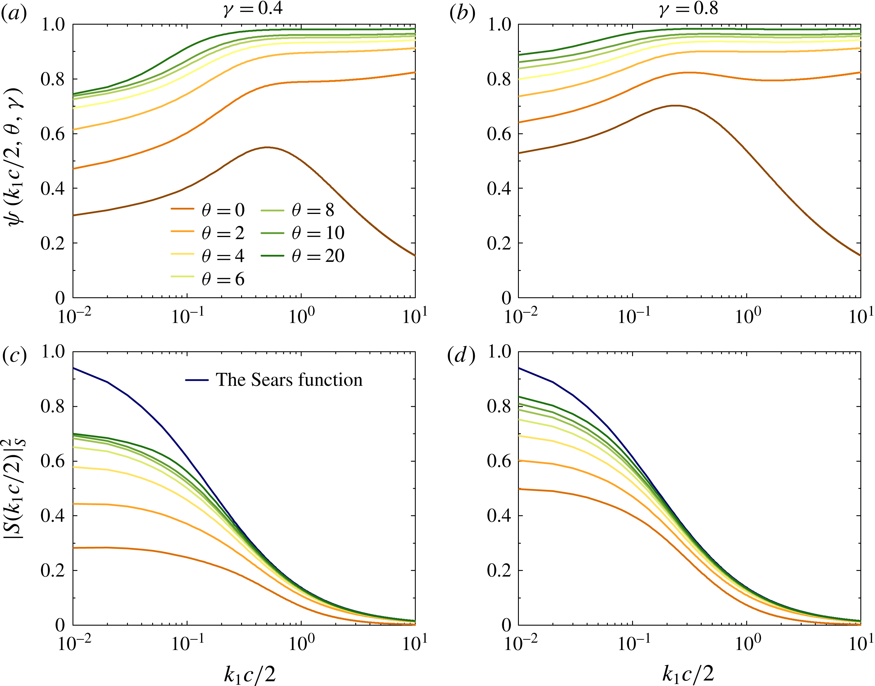
. Now we give some numerical examples for a series of aspect ratios and two ratios of the vertical integral scale to the chord. From the results shown in figures 3(a) and 3(b), the ratio
 $\unicode[STIX]{x1D713}$
at high frequencies can be easily increased by increasing the aspect ratio. At a small ratio of the vertical integral scale to the chord, the ratio
 $\unicode[STIX]{x1D713}$
at low frequencies can be increased to a certain extent by increasing the aspect ratio. With a continued increase of the aspect ratio, there is a limited effect of increasing the ratio
 $\unicode[STIX]{x1D713}$
. To make the ratio
 $\unicode[STIX]{x1D713}$
at low frequencies closer to 1, the ratio of the turbulence integral scale to the chord is required to take larger values. The same conclusions can be obtained from the results of figures 3(c) and 3(d).
The values of the ratio
 $\unicode[STIX]{x1D713}$
and the theoretical one-wavenumber transfer function obtained from the strip assumption
 $|S(k_{1}c/2)|_{s}^{2}$
for different aspect ratios
 $\unicode[STIX]{x1D703}$
and different ratios of the vertical integral scale to the chord
 $\unicode[STIX]{x1D6FE}$
.

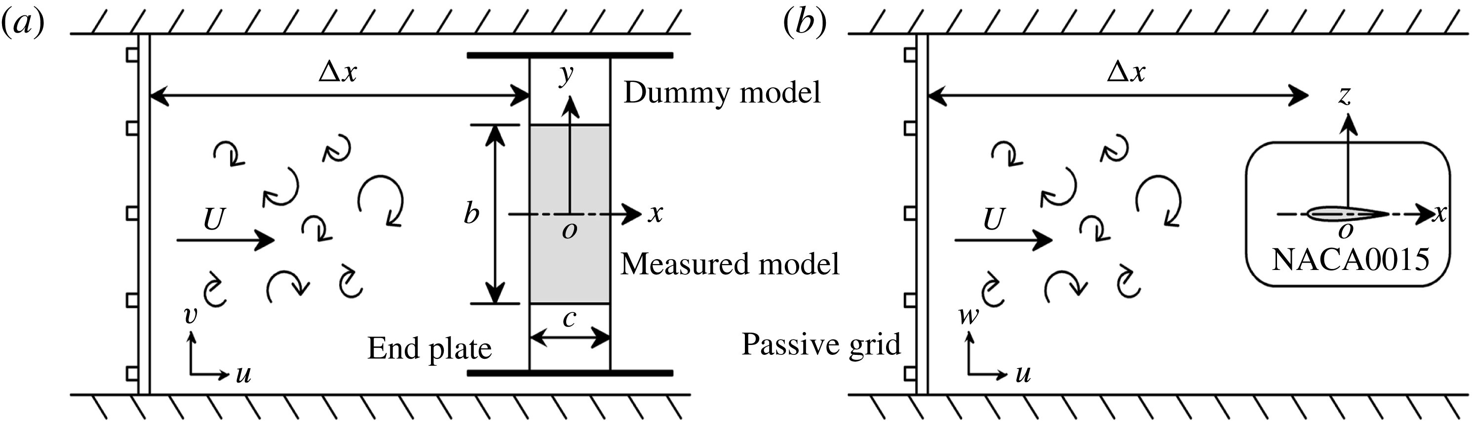
The experimental set-up of a stationary rectangular wing encountering a turbulent flow generated by a square passive grid: (a) top view; (b) side view.

3 Experimental arrangements
The experiments are conducted in a closed-loop wind tunnel (XNJD-1) at Southwest Jiaotong University, the same as that used in Li et al. (Reference Li, Li and Liao2015). Figure 4 shows a sketch of the experimental set-up: a stationary wing is submitted to a turbulent flow generated by a square passive grid. The tunnel has a
 $2.4~\text{m (width)}\times 2~\text{m (height)}$
test section. A grid with a mesh size of 0.33 m and a square bar of width 0.07 m is installed downstream of the entrance to the test section. The instantaneous velocities of the flow field are measured by a TFI Cobra Probe. The Cobra Probe is a multi-hole pressure probe able to resolve 3 components of velocity with an estimated uncertainty of
 $\pm 0.1~\text{m}~\text{s}^{-1}$
, which has a frequency response of 0 Hz up to more than 2000 Hz. Three rectangular wing models with different aspect ratios (
 $b=0.48$
, 0.8 and 1.12 m,
 $c=0.16~\text{m}$
) are used. These wing models have a NACA 0015 profile cross-section and are made of glass fibre with several transverse ribs to increase the necessary flexural rigidity. The distance from the leading edge of the wing to the grid is approximately
 $\unicode[STIX]{x0394}x=4.2~\text{m}$
. To prevent the air stream from being able to flow around the tips and to approximate the infinite wing condition, two dummy models are installed at two sides of the measured model while two end plates are installed at each end of the dummy model. The models are mounted horizontally at zero angle of attack on a force-measured balance device. The balance consists of two ATI Nano17 six-axis sensors with an accuracy of 0.0125 N. The outputs of these two sensors are summed to a total signal using a synchronous data acquisition system. The external noise contained in the original signal is filtered by Chebyshev filter. The spectrum of the signal is obtained using the pwelch spectral estimation. The lowest resonant frequency of the model mounted on the balance is 90 Hz. To remove the resonant peak of the force spectrum, a single degree of freedom mechanical admittance is used. In addition, in order to judge the data accurately, the insignificant isolated points are carefully eliminated. In the experiments, the data of the lift force and instantaneous velocity are recorded at a same sampling frequency of 1024 Hz, the durations of measurements are 60 s, the main flow velocity is adjusted to
 $U=13.5~\text{m}\,\text{s}^{-1}$
, the corresponding Reynolds number based on the chord length is
 $Re=144\,000$
.
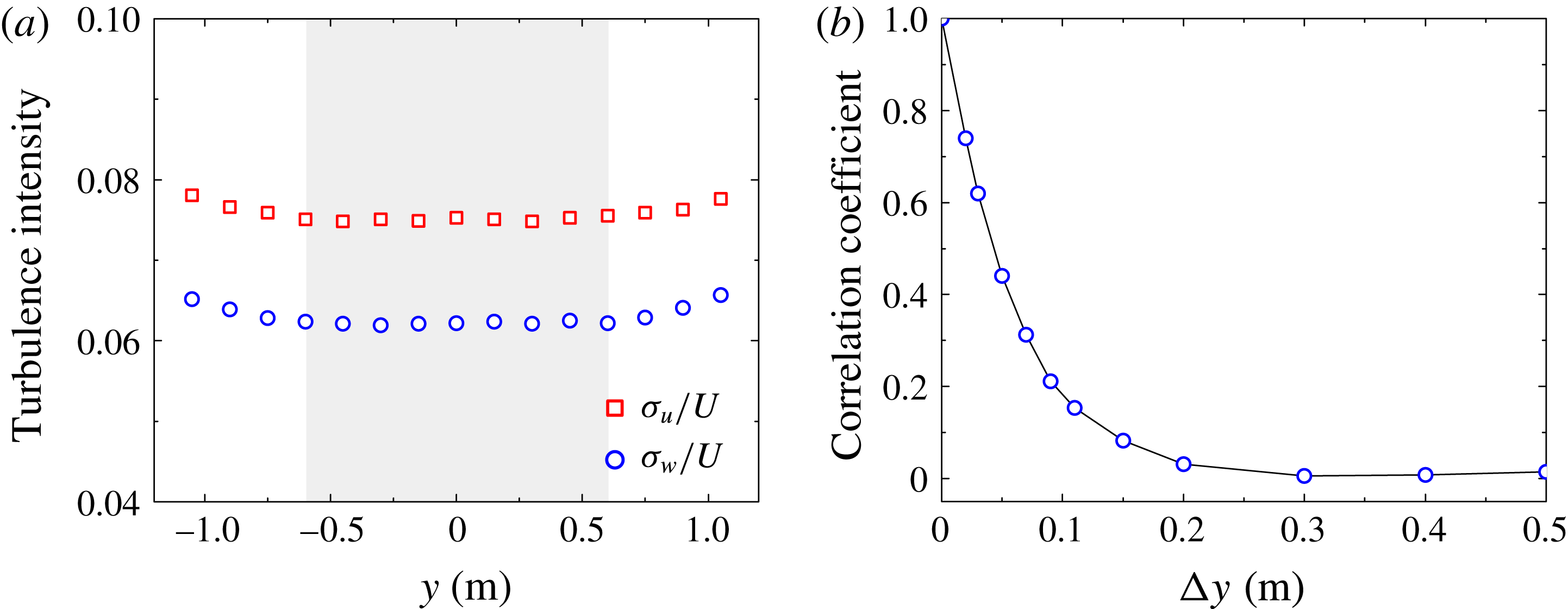
(a) The spanwise distributions of turbulence intensities,
 $\unicode[STIX]{x1D70E}_{u}/U$
and
 $\unicode[STIX]{x1D70E}_{w}/U$
; (b) the spanwise correlation coefficient of the vertical velocity fluctuation,
 $g_{w}(\unicode[STIX]{x0394}y)$
.
 $\unicode[STIX]{x0394}y$
is the spanwise distance. The measurement region is highlighted with a grey background.

4 Experimental results and discussions
4.1 Characteristics of the grid turbulence
In this study, the behaviour of large-scale structures of the turbulent flow is important for the measurement results. Thus we first ensure that the measurement region is not affected by the side wall. As is shown in figure 5(a), the side wall effects are negligible and good homogeneity can be confirmed in the measurement region. For isotropic turbulence, the turbulence intensities
 $\unicode[STIX]{x1D70E}_{u}/\unicode[STIX]{x1D70E}_{w}$
should be unity everywhere, where
 $\unicode[STIX]{x1D70E}_{u}$
and
 $\unicode[STIX]{x1D70E}_{w}$
are the root mean squares of longitudinal and vertical velocity fluctuations, respectively. In this experiment,
 $\unicode[STIX]{x1D70E}_{u}/U=0.074$
,
 $\unicode[STIX]{x1D70E}_{w}/U=0.063$
. The ratio
 $\unicode[STIX]{x1D70E}_{u}/\unicode[STIX]{x1D70E}_{w}$
is approximately 1.17.
 $\unicode[STIX]{x1D70E}_{u}$
is slightly larger than
 $\unicode[STIX]{x1D70E}_{w}$
, as observed in previous grid turbulence experiments (Comte-Bellot & Corrsin Reference Comte-Bellot and Corrsin1966; Lavoie, Djenidi & Antonia Reference Lavoie, Djenidi and Antonia2007; Kitamura et al.
Reference Kitamura, Nagata, Sakai and Harasaki2014). The turbulence integral scale, defined as the integration of the correlation coefficient, represents the characteristic length of the turbulence. In practical measurements, the vertical integral scale in the streamwise direction,
 $L_{w}^{x}$
, is usually determined by comparison with the measured one-wavenumber turbulence spectrum. In this matching, the one-wavenumber von Kármán spectral model which is integrated from equation (2.9) can be used. It is
 $$\begin{eqnarray}\displaystyle & \displaystyle \unicode[STIX]{x1D719}_{w}(k_{1})={\displaystyle \frac{4\unicode[STIX]{x1D70E}_{w}^{2}L_{w}^{x}[1+(8/3)(2.678L_{w}^{x}k_{1})^{2}]}{[1+(2.678L_{w}^{x}k_{1})^{2}]^{11/6}}}. & \displaystyle\end{eqnarray}$$
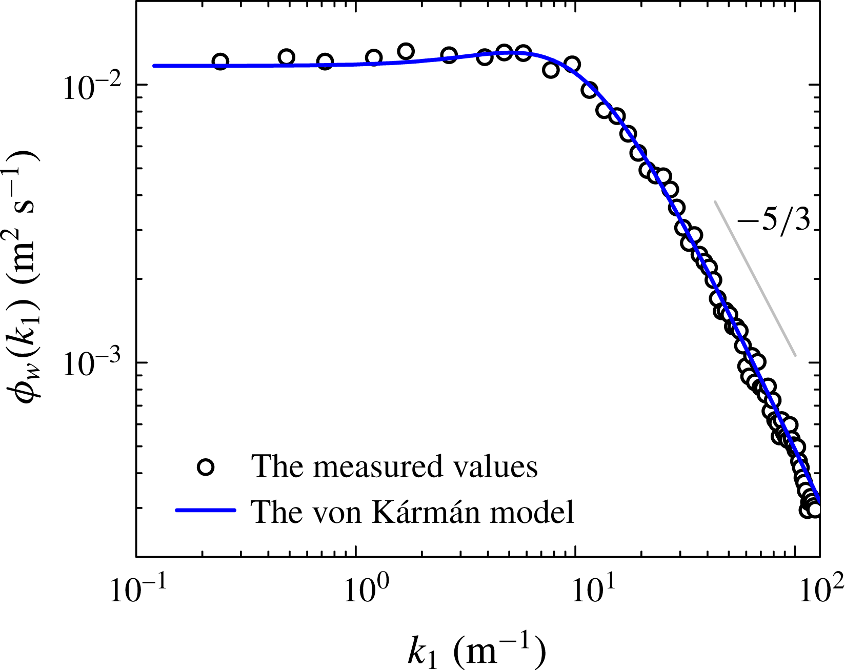
Figure 6 shows the measured one-wavenumber spectrum of the vertical velocity fluctuation. It can be seen that the measured results agree with the one-wavenumber von Kármán spectral model. The vertical integral scale in the streamwise direction, which is determined from the one-wavenumber turbulence spectral model,
 $L_{w}^{x}$
, is 0.052 m. To better assess the isotropy of the experimental grid turbulence, the vertical integral scale in the spanwise direction is also given. It is obtained by integrating the spanwise correlation coefficient of the vertical velocity fluctuation,
 $g_{w}(\unicode[STIX]{x0394}y)$
, as is shown in figure 5(b). The vertical integral scale in the spanwise direction, which is calculated from the definition,
 $L_{w}^{y}$
, is 0.049 m. The ratio
 $L_{w}^{x}/L_{w}^{y}$
is approximately 1.06,
 $L_{w}^{y}$
is slightly smaller than
 $L_{w}^{x}$
. These characteristics of the grid turbulence indicate that the present grid turbulent flow field could be regarded to be approximately isotropic.
The one-wavenumber spectrum of the vertical velocity fluctuation, the experimental values indicated by marker symbols are compared with the theoretical curve of the one-wavenumber von Kármán spectral model.

4.2 Ratio
 $\unicode[STIX]{x1D713}$
and span-correction factor
$\unicode[STIX]{x1D711}$


The ratio of the vertical integral scale (in the streamwise direction) to the chord
 $\unicode[STIX]{x1D6FE}$
is 0.32. The aspect ratios
 $\unicode[STIX]{x1D703}$
, as stated in § 3, are 3, 5 and 7. Substituting these two parameters into equations (2.10) and (2.12), the ratio
 $\unicode[STIX]{x1D713}$
and the span-correction factor
 $\unicode[STIX]{x1D711}$
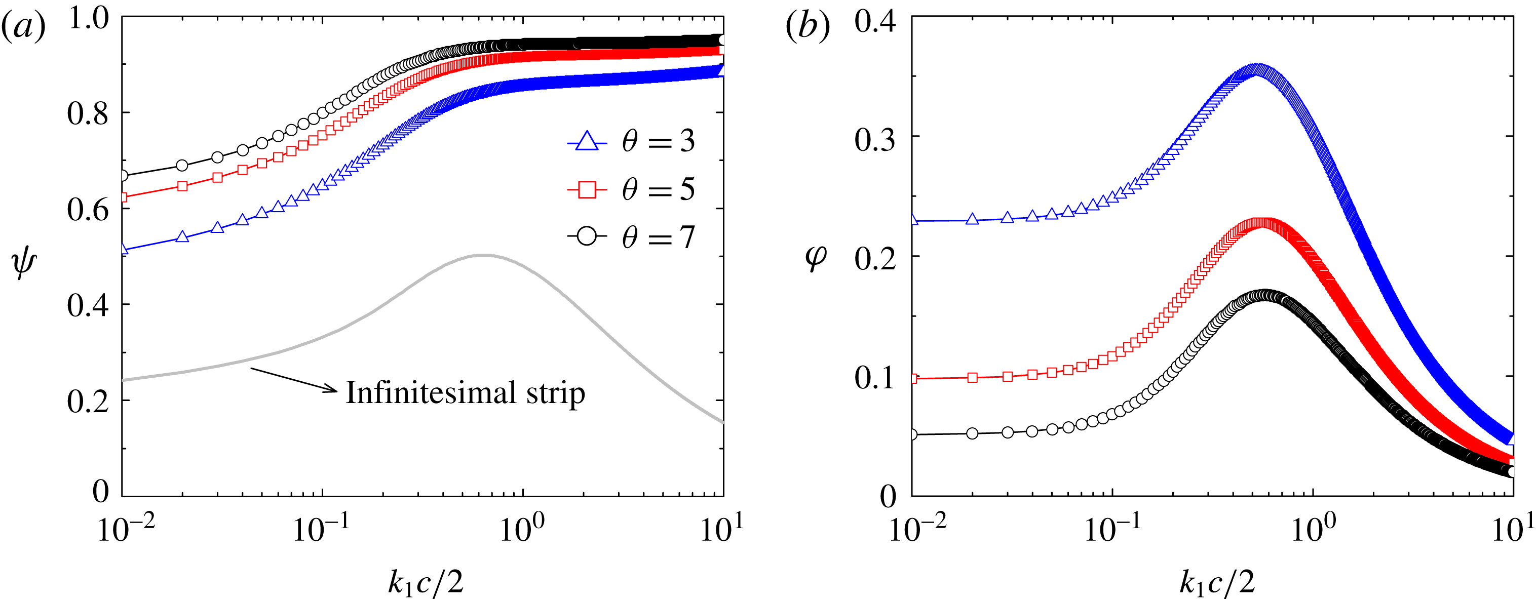
used in this experiment are then obtained. Figure 7(a) shows the ratio
 $\unicode[STIX]{x1D713}$
for
 $\unicode[STIX]{x1D703}=3$
, 5, 7 and
 $\unicode[STIX]{x1D6FE}=0.32$
. For comparison, the ratio
 $\unicode[STIX]{x1D713}$
for
 $\unicode[STIX]{x1D6FE}=0.32$
and
 $\unicode[STIX]{x1D703}\rightarrow 0$
(the infinitesimal strip) is also included. Figure 7(b) shows the span-correction factor
 $\unicode[STIX]{x1D711}$
for
 $\unicode[STIX]{x1D703}=3$
, 5, 7 and
 $\unicode[STIX]{x1D6FE}=0.32$
.
(a) The ratio
 $\unicode[STIX]{x1D713}$
; (b) the span-correction factor
 $\unicode[STIX]{x1D711}$
.
 $\unicode[STIX]{x1D6FE}=0.32$
.

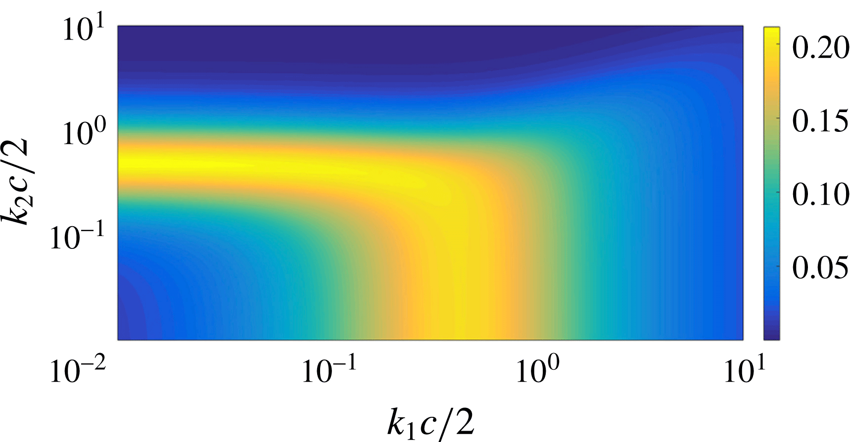
The two-wavenumber coherence function of the vertical velocity fluctuation
 $R_{w}$
.

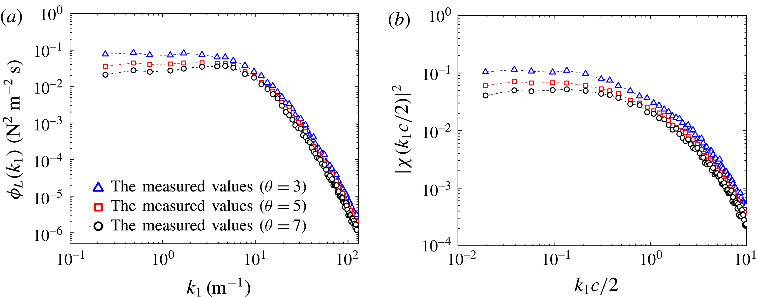
(a) The measured one-wavenumber spectra of lift forces per unit span of three wings with different aspect ratios; (b) the corresponding measured generalized transfer functions.

The characteristics of
 $\unicode[STIX]{x1D713}$
and
 $\unicode[STIX]{x1D711}$
may be influenced by the spanwise spatial distribution of the turbulence structure, which could be characterized by the two-wavenumber coherence function in the wavenumber space (see the appendix A). From figures 7 and 8, it can be seen that the curves of
 $\unicode[STIX]{x1D713}$
and
 $\unicode[STIX]{x1D711}$
vary with the two-wavenumber coherence function. The larger the coherence function is, the more spanwise correlated the turbulent flow structure is, and the less the influence of the spanwise wavenumber is. The curves of
 $\unicode[STIX]{x1D713}$
and
 $\unicode[STIX]{x1D711}$
reflect the influence of the spanwise wavenumber (note that these curves are the results of the integral of the spanwise wavenumber). Thus these curves reach a peak at the frequency of the most correlated wavenumber region of the turbulent flow structure, and then decrease as the frequency increases. However, with increasing aspect ratio, the influence of the spanwise wavenumber contained in
 $\unicode[STIX]{x1D713}$
is gradually eliminated, this trend is weakened correspondingly, as is shown in figure 7(a).
4.3 One-wavenumber transfer function obtained from the strip assumption
The measured one-wavenumber spectra of lift forces per unit span of three wings with different aspect ratios are shown in figure 9(a). The corresponding measured generalized transfer functions are shown in figure 9(b). Substituting the measured generalized transfer functions and
 $\unicode[STIX]{x1D711}$
into equation (2.16), the experimental one-wavenumber transfer functions obtained from the strip assumption are determined. Substituting the Sears function and
 $\unicode[STIX]{x1D713}$
into equation (2.20), the corresponding theoretical predictions are obtained.
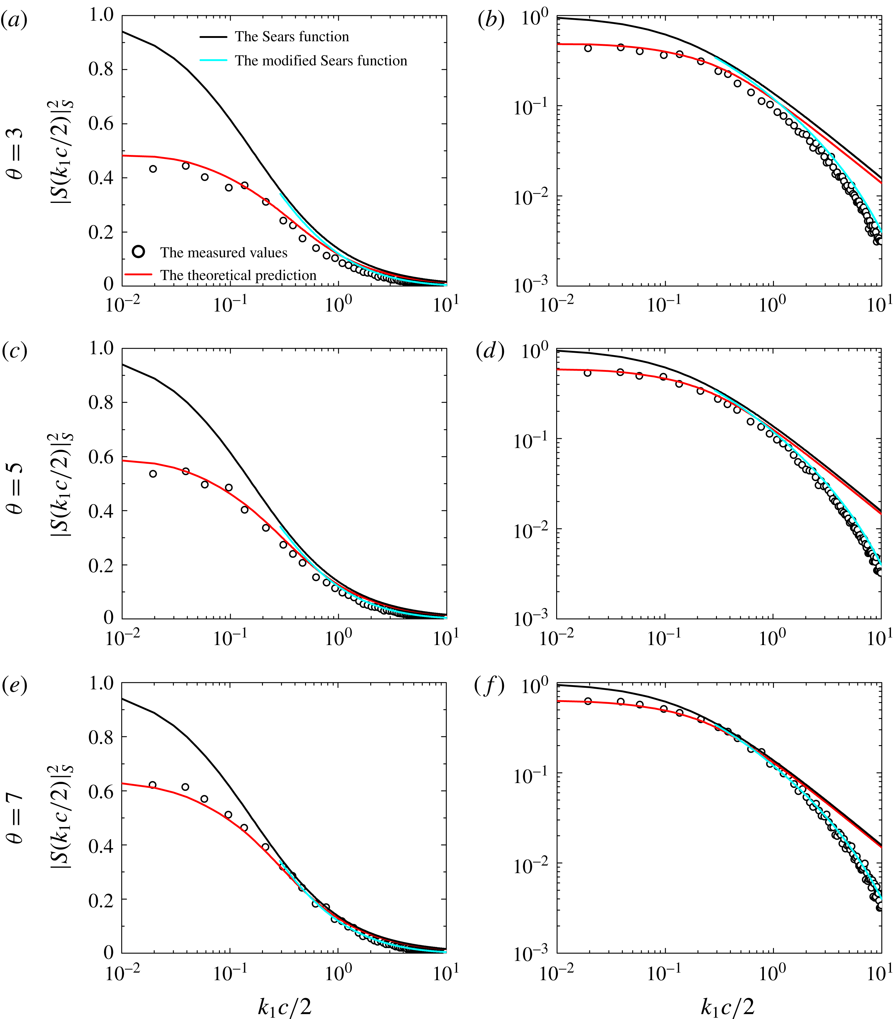
The one-wavenumber transfer function obtained from the strip assumption
 $|S(k_{1}c/2)|_{s}^{2}$
of three wings with different aspect ratios.
 $\unicode[STIX]{x1D6FE}=0.32$
.

As is shown in figure 10, the experimental one-wavenumber transfer functions obtained from the strip assumption agree with the corresponding theoretical predictions at low frequencies. In this frequency range, the values of
 $\unicode[STIX]{x1D713}$
are small, the experimental one-wavenumber transfer function obtained from the strip assumption falls below the Sears function. With increasing aspect ratio, the value of the ratio
 $\unicode[STIX]{x1D713}$
increases, the accuracy of the strip assumption is improved and the deviation between the experimental one-wavenumber transfer function obtained from the strip assumption and the Sears function is reduced. Here, the turbulence integral scale to the chord ratio used is relatively small, the role of the aspect ratio in the improvement of the accuracy of the strip assumption at low frequencies seems to be limited. To further improve the accuracy of strip assumption, or say, to make the experimental one-wavenumber transfer function obtained from the strip assumption closer to the Sears function at low frequencies, the ratio of the turbulence integral scale to the chord should be larger. Meanwhile, the experimental values for all wing models tend to be consistent as the frequency increases, which is the same trend as for the ratio
 $\unicode[STIX]{x1D713}$
. This means that the strip assumption would be quite accurate at high frequencies when the aspect ratio has moderate values, even if the ratio of the turbulence integral scale to the chord is small.
The testing results also show that the experimental values at high frequencies fall off faster than the Sears function, although the influence of the spanwise wavenumber has been almost eliminated. This phenomenon may be caused by the thickness of the NACA 0015 airfoil cross-section used in the experiment. It is known that the Sears function is derived based on the flat plate assumption. Under this assumption, the mean flow around the wing is considered to be a uniform parallel flow, and therefore the eddy (or gust component) of the incident turbulent flow is not affected by the surrounding mean flow velocity field. In fact, when the cross-section of the wing has a thickness, camber or angle of attack, the surrounding mean flow velocity field is disturbed, varying with the spatial position. If the gust component of the turbulent flow passes through such a spatially variable velocity field, its characteristics will be altered. The work of Goldstein & Atassi (Reference Goldstein and Atassi1976) indicated that the mechanism of this phenomenon can be explained with the second-order theory. When considering the second-order approximation of the kinematic boundary condition due to the disturbed mean flow velocity, the gust is shown to be distorted. In this case, the transfer function is dependent not only on the vertical velocity fluctuation but also on the longitudinal velocity fluctuation, which is less than the Sears function as the frequency increases. In addition, Atassi (Reference Atassi1984) pointed out that, in spite of the nonlinear dependence of the unsteady flow on the mean flow, the effects of gust distortion on the transfer function can be linearly decomposed into three independent components which account separately for the effects of the airfoil thickness, airfoil camber and angle of attack. For the convenience of routine calculation, the effect of thickness is usually accounted for by modifying the Sears function with a simple thickness correction factor (Gershfeld Reference Gershfeld2004). Here, the modified form of the Sears function suggested by Lysak et al. (Reference Lysak, Capone and Jonson2013) is employed to compare with the experimental values at high frequencies. Lysak’s modified form includes a quasi-steady correction factor and an exponential attenuation correction factor. It is
 $$\begin{eqnarray}\displaystyle & \displaystyle \left|S\left({\displaystyle \frac{k_{1}c}{2}}\right)\right|_{mod}^{2}=\left(1+\unicode[STIX]{x1D700}+{\displaystyle \frac{\unicode[STIX]{x1D6FF}_{te}}{2\unicode[STIX]{x03C0}}}\right)^{2}\text{e}^{-\unicode[STIX]{x1D6FD}(\unicode[STIX]{x1D70F})k_{1}c/2\unicode[STIX]{x03C0}}\left|S\left({\displaystyle \frac{k_{1}c}{2}}\right)\right|^{2}. & \displaystyle\end{eqnarray}$$
The first term is the quasi-steady lift correction factor, the second term is the exponential attenuation factor,
 $\unicode[STIX]{x1D700}$
is the conformal mapping thickness parameter,
 $\unicode[STIX]{x1D6FF}_{te}$
is the trailing edge angle,
 $\unicode[STIX]{x1D6FD}(\unicode[STIX]{x1D70F})$
is the curve fit parameter which controls the rate of high frequency attenuation,
 $\unicode[STIX]{x1D70F}$
is the airfoil thickness.
From the results, it can be seen that, contrary to Sears’ flat plate transfer function, which does not capture the experimental values at high frequencies, Lysak’s modified form of the Sears function, which takes the effect of airfoil thickness into account, agrees well with the experimental values. Here, it is worth noting that the distortion of the incident turbulent flow due to the thickness will also cause a decrease in the fluctuating velocity spatial correlations within the vicinity of the wing (Santana et al. Reference Santana, Christophe, Schram and Desmet2016). From the point of view of the frequency domain, this distortion of the small-scale eddy causes a decrease of the coherence of the incident velocity fluctuations at high frequencies, and consequently may result in a decrease of the coherence of the lift forces. However, it is believed that the fundamental properties of the results would not be lost because of this. In this case, it is not difficult to infer that the actual two-wavenumber influence factor of the transfer function will be lower than the theoretical values. For the same group of scale to chord ratio and aspect ratio, the actual ratio evaluating the accuracy of the strip assumption will be larger than the theoretical ratio at high frequencies, and thus the experimental values of the one-wavenumber transfer function may be closer to the modified form of the Sears function. Nevertheless, to extend the application of the proposed theory, more extensive and systematic measurements involving several other configurations would be very worthwhile.
5 Conclusions
This paper has investigated the applicability of the strip assumption in the estimation of the unsteady lift response of a two-dimensional wing in turbulent flow. Firstly, the ratio between the lift spectrum calculated from the two-wavenumber analysis and the lift spectrum calculated from the strip assumption is used to evaluate the accuracy of the strip assumption, showing that the controlling parameters are the ratio of the turbulence integral scale to the chord and the aspect ratio. Secondly, the theoretical analysis is confirmed by investigating the relationship between the one-wavenumber transfer function obtained from the strip assumption and the Sears function. Both the theoretical and experimental results show that, as the controlling parameters increase, the ratio evaluating the accuracy of the strip assumption increases, the one-wavenumber transfer function obtained from the strip assumption becomes closer to the Sears function. It could be concluded from this work that the accuracy of the strip assumption could be improved by increasing the ratio of the turbulence integral scale to the chord and the aspect ratio, thus the strip assumption could be used within an acceptable error margin when these two parameters have suitable values. In particular, for the case of high aspect ratio wings in atmospheric turbulence (neglecting the tip effects), the strip assumption may be accurate enough to enable the Sears function to be used to estimate the unsteady lift response of the wing. In fact, this also provides a simple approach for direct measurement of the Sears function (or other one-wavenumber transfer functions for other slender structures) in turbulent flow. In this approach, the measurement of the Sears function only requires the one-wavenumber spectrum of the vertical velocity fluctuation and of the unsteady lift, without the two-wavenumber analysis. The accuracy of the obtained Sears function depends on the value of the ratio evaluating the accuracy of the strip assumption. On the other hand, the experiments also reveal that caution should be exercised when using the Sears function to estimate the unsteady lift response at high frequencies. For a wing of thick-airfoil cross-section, the effect of thickness will lead to the flat plate assumption being invalid at high frequencies, and therefore the Sears function, which is derived based on the flat plate assumption, cannot correctly estimate the unsteady lift response at high frequencies. In practical situations, the effect of thickness on the transfer function should be taken into account. The use of the exponential attenuation correction factor appears to be an appropriate approach.
Acknowledgements
The present work is supported by National Natural Science Foundation under Grant Nos. 51478402, 51608074. We are indebted to Dr N. Yeung (ARUP, Hong Kong) for his valuable comments and suggestions, which greatly enhanced the quality of this paper.
Appendix A
Based on the von Kármán model, the coherence function of the vertical velocity fluctuation expressed in terms of the spanwise distance is (Roberts & Surry Reference Roberts and Surry1973)
 $$\begin{eqnarray}\displaystyle & \displaystyle \text{Coh}_{w}(k_{1},\unicode[STIX]{x0394}y)={\displaystyle \frac{2^{1/6}}{\unicode[STIX]{x1D6E4}(5/6)}}\left[\unicode[STIX]{x1D70D}^{5/6}\text{K}_{5/6}(\unicode[STIX]{x1D70D})-{\displaystyle \frac{\unicode[STIX]{x1D70D}^{11/6}}{1+32/3(1/C)^{2}(L_{w}^{x}k_{1})^{2}}}\text{K}_{1/6}(\unicode[STIX]{x1D70D})\right], & \displaystyle\end{eqnarray}$$
 $$\begin{eqnarray}\displaystyle & \displaystyle \unicode[STIX]{x1D70D}={\displaystyle \frac{\unicode[STIX]{x0394}y}{2L_{w}^{x}}}\sqrt{C^{2}+4(k_{1}L_{w}^{x})^{2}}, & \displaystyle\end{eqnarray}$$
 $$\begin{eqnarray}\displaystyle & \displaystyle C=\sqrt{\unicode[STIX]{x03C0}}{\displaystyle \frac{\unicode[STIX]{x1D6E4}(5/6)}{\unicode[STIX]{x1D6E4}(1/3)}}. & \displaystyle\end{eqnarray}$$
 $\text{K}_{1/6}$
and
 $\text{K}_{5/6}$
are the Bessel functions of the second kind. Using Fourier transformation, the two-wavenumber coherence function of the vertical velocity fluctuation can be then written as follow
 $$\begin{eqnarray}\displaystyle & \displaystyle R_{w}(k_{1},k_{2})={\displaystyle \frac{2\unicode[STIX]{x1D6E4}(4/3)}{\unicode[STIX]{x1D6E4}(5/6)}}\sqrt{\unicode[STIX]{x03C0}}A^{5/3}\left\{{\displaystyle \frac{[1+5/(3B)]k_{2}^{2}+(1-1/B)A^{2}}{[k_{2}^{2}+A^{2}]^{7/3}}}\right\}, & \displaystyle\end{eqnarray}$$
 $$\begin{eqnarray}\displaystyle & \displaystyle A={\displaystyle \frac{1}{2L_{w}^{x}}}\sqrt{C^{2}+4(k_{1}L_{w}^{x})^{2}}, & \displaystyle\end{eqnarray}$$
 $$\begin{eqnarray}\displaystyle & \displaystyle B=1+{\displaystyle \frac{32(k_{1}L_{w}^{x})^{2}}{3C^{2}}}, & \displaystyle\end{eqnarray}$$
 $$\begin{eqnarray}\displaystyle & \displaystyle C=\sqrt{\unicode[STIX]{x03C0}}{\displaystyle \frac{\unicode[STIX]{x1D6E4}(5/6)}{\unicode[STIX]{x1D6E4}(1/3)}}. & \displaystyle\end{eqnarray}$$