

1. Introduction
In this study, we investigate the dynamics of the full nonlinear evolution and collision of magneto-quasi-geostrophic (MQG) modons on the
 $f$
-plane. The term ‘modon’, introduced in Stern (Reference Stern1975), refers to a coherent, localised vortex structure characterised by a pair of counter-rotating cyclonic and anticyclonic regions that propagate steadily. These structures are distinguished by their form-preserving nature and uniform propagation. The classical modon solutions originally formulated within the ‘ordinary’ quasi-geostrophic (QG) framework in Larichev & Reznik (Reference Larichev and Reznik1976) were inspired by Lamb’s dipole in two-dimensional hydrodynamics. Over the past five decades, the durability and steady propagation of vortical structures such as modons and eddies have garnered significant attention in the fields of ocean and atmospheric dynamics, alongside efforts to develop modon theories (see Flierl et al. Reference Flierl, Larichev, McWilliams and Reznik1980; Tribbia Reference Tribbia1984; Reznik Reference Reznik1987; Kizner Reference Kizner1988, Reference Kizner1997; Nycander Reference Nycander1988; Khvoles, Berson & Kizner Reference Khvoles, Berson and Kizner2005; Hughes & Miller Reference Hughes and Miller2017; Yano & Tribbia Reference Yano and Tribbia2017). Additionally, modon solutions have been developed within the thermal quasi-geostrophic regime of the rotating shallow water model, which accounts for horizontal density and temperature gradients (Lahaye, Zeitlin & Dubos Reference Lahaye, Zeitlin and Dubos2020). In equatorial regions, modons are exact, form-preserving nonlinear solutions to the inviscid QG equations, characterised by their horizontal localisation and consistent eastward translation (see Tribbia Reference Tribbia1984; Rostami & Zeitlin Reference Rostami and Zeitlin2019a, Reference Rostami and Zeitlin2021). These modons can also arise from equatorial adjustment processes involving large-scale disturbances in the moist-convective rotating shallow water model, a novel approach introduced in Rostami & Zeitlin (Reference Rostami and Zeitlin2019b). This concept was subsequently employed to develop a theory for the genesis and dynamics of Madden–Julian oscillations (Rostami, Zhao & Petri Reference Rostami, Zhao and Petri2022).
Recent theoretical advances in Lahaye & Zeitlin (Reference Lahaye and Zeitlin2022) have extended classic modon solutions within the QG framework to incorporate magnetic effects on the
 $f$
-plane, where f is the constant Coriolis parameter representing the effect of Earth’s rotation. This study builds upon that foundational work by further developing the dynamics of MQG modons using the magnetohydrodynamic rotating shallow water (MRSW) model. Specifically, we revisit the problem of the single modon dynamics and its stability, originally explored in Lahaye & Zeitlin (Reference Lahaye and Zeitlin2022), with a novel numerical approach. Our computations employ an upgraded numerical scheme – the locally divergence-free, well-balanced, path-conservative central-upwind scheme recently introduced in Chertock et al. (Reference Chertock, Kurganov, Redle and Zeitlin2024) – which enables higher resolution, longer integration times and improved preservation of physical invariants. A key strength of this scheme lies in its ability to capture wave interactions, maintain steady states even in the presence of sharp gradients and ensure magnetic field divergence-free constraints at the discrete level. Subsequently, we study different scenarios involving collisions and interactions of MQG modons, providing new insights into their nonlinear dynamics and long-term evolution.
The MRSW model, introduced in Gilman (Reference Gilman2000), provides a conceptual framework for examining the solar tachocline – a shear layer between the Sun’s convective zone and its radiative interior (Spiegel & Zahn Reference Spiegel and Zahn1992). Estimates indicate that approximately two thirds of the tachocline lies within the radiative zone, while one third resides in the overshoot zone (Charbonneau et al. Reference Charbonneau, Christensen-Dalsgaard, Henning, Larsen, Schou, Thompson and Tomczyk1999). By integrating magnetohydrodynamic (MHD) effects into classical shallow water theory, the MRSW model utilises vertical averaging across magnetic surfaces and applies the mean-field approximation to simplify the full set of primitive MHD equations under MHD equilibrium. Traditional shallow water models, in the absence of magnetic fields, describe a homogeneous, incompressible fluid in hydrostatic balance (Zeitlin Reference Zeitlin2018).
Using the MRSW model, Magill et al. (Reference Magill, Coutino, Storer, Stastna and Poulin2019) studied the evolution of an initial vortex into two zonally propagating, doughnut-shaped vortices (nonlinear Alfvén waves). They demonstrated that, at high rotation rates, akin to those of rapidly spinning stars, these Alfvén waves retained their structural integrity outside of collisions. It is worth noting that other studies have reported solitary wave solutions in the MRSW model. London (Reference London2017) derived equatorial magneto-Rossby solitary waves within the shallow water MHD framework under varying strengths of ambient toroidal magnetic fields. These solutions, obtained using a multiple-scale asymptotic technique, extend the classic equatorial Rossby soliton solutions to MHD contexts. In a different setting, Hori, Tobias & Jones (Reference Hori, Tobias and Jones2020) investigated finite-amplitude hydromagnetic Rossby waves in the magnetostrophic regime within spherical shells. They found that weakly nonlinear slow waves evolve according to the Korteweg–de Vries equation, leading to soliton solutions that may manifest as coherent structures, such as isolated anticyclones.
The MRSW model transitions to a system of MQG equations through an asymptotic expansion for small Rossby and magnetic Rossby numbers – indicative of strong rotational dominance – filtering out high-frequency waves and isolating the dynamically relevant modes. The MQG approximation, derived from broader QG theory, is pivotal for studying quasi-two-dimensional MHD turbulence, particularly in solar and astrophysical contexts (Tobias, Diamond & Hughes Reference Tobias, Diamond and Hughes2007).
In this paper, we conduct a series of numerical experiments to investigate the nonlinear dynamical evolution, dispersion characteristics and stability metrics of magnetic modons on the
 $f$
-plane. The simulations have been performed using the locally divergence-free well-balanced path-conservative central-upwind scheme recently introduced in Chertock et al. (Reference Chertock, Kurganov, Redle and Zeitlin2024). This scheme is second-order accurate and very robust due to its important features that guarantee the magnetic field divergence-free property, a proper balancing of the flux and source terms allowing us to exactly preserve several physically relevant equilibria and a proper treatment of non-conservative product terms thanks to the implementation of the path-conservative integration technique. The obtained simulation results reveal that the stability of these coherent vortex structures is critically dependent on the spatial intensity and distribution of the magnetic field, both within and in the vicinity of the dipolar configuration. We further elucidate how interactions between analogous and antithetical magnetic fields facilitate the merging and subsequent formation of enduring tripolar and checkered magnetic patterns. These emergent structures, resulting from the interplay of magnetic dipoles, display persistence and dynamical coherence, demonstrating their robustness against perturbations and their ability to maintain structured magnetic configurations over extended periods. It is important to emphasise that the initialised magnetic modons in this study are not parametrised to be directly mapped onto the solar tachocline. Rather, this work provides a theoretical exploration of modons in a general plasma setting, offering insights relevant to a range of astrophysical environments, including the Sun, but without the explicit goal of modelling the tachocline itself at this stage. Notably, dipolar vortex structures have been observed in other plasma contexts, including magnetised dusty plasmas, where they may arise due to the nonlinear saturation of Kelvin–Helmholtz instability (Rawat & Rao Reference Rawat and Rao1993; Shukla & Rao Reference Shukla and Rao1993; Jovanović & Shukla Reference Jovanović and Shukla2001; Ijaz, Mirza & Azeem Reference Ijaz, Mirza and Azeem2007). These similarities suggest broader implications for modon dynamics beyond the specific framework of geophysical and astrophysical fluid dynamics.
The paper is organised as follows. In § 2, we describe the model and the governing equations used in this study. Section 3 presents the evolution of magnetic modons in the
 $f$
-plane, detailing the nonlinear dynamics of different modon configurations. In § 4, we investigate the interactions and collisions between two magnetic modons. Finally, the conclusions drawn from this study are summarised in § 5.
2. Description of MRSW model and magnetic modon solutions
The MRSW model equations in the rotating
 $(x, y)$
plane are
 \begin{align}& \boldsymbol{v}_t+\boldsymbol{v\cdot \nabla }\boldsymbol{v}+f\hat {\boldsymbol{z}}\times \boldsymbol{v}+ g\nabla h=\frac {1}{h}\nabla \cdot (h\boldsymbol{b}\otimes \boldsymbol{b}), \end{align}
 \begin{align}&\qquad\qquad\quad h_t+\nabla \cdot (h\boldsymbol{v})=0, \end{align}
 \begin{align}&\qquad\qquad\qquad \nabla \cdot (h\boldsymbol{b})=0, \end{align}
 \begin{align}&\qquad\quad \boldsymbol{b}_t+\boldsymbol{v\cdot \nabla }\boldsymbol{b}=\frac {1}{h}\nabla \cdot (h\boldsymbol{v}\otimes \boldsymbol{b}). \end{align}
Here,
 $f$
is the Coriolis parameter accounting for planetary rotation,
 $g$
is the gravitational acceleration and the key dynamical variables include the layer thickness
 $h$
, velocity field
 $\boldsymbol{v}=u\hat {\boldsymbol{x}}+v\hat {\boldsymbol{y}}$
and magnetic field
 $\boldsymbol{b}=a\hat {\boldsymbol{x}}+b\hat {\boldsymbol{y}}$
. The unit vectors
 $(\hat {\boldsymbol{x}},\hat {\boldsymbol{ y}},\hat {\boldsymbol{z}})$
correspond to the Cartesian axes and
 $\nabla$
represents the spatial gradient operator. The magnetic field
 $\boldsymbol{b}$
is non-dimensionalised to have the same dimensions as the velocity field, representing the Alfvén velocity, through the scaling by vacuum permeability and fluid density. The tensor notation
 $\nabla \cdot (\boldsymbol{A}\otimes \boldsymbol{B})$
indicates the divergence of the outer product of vectors
 $\boldsymbol{A}$
and
 $\boldsymbol{B}$
. The Coriolis parameter
 $f=f_0+\beta y$
is constant in the
 $f$
-plane configuration and varies linearly with latitude
 $y$
in the
 $\beta$
-plane configuration (in this study, we restrict our consideration to the case
 $f\equiv f_0$
),
 $\beta$
represents the meridional gradient of the Coriolis parameter due to Earth’s spherical geometry. The divergence-free constraint (2.3) is satisfied by introducing a scalar magnetic potential
 $A$
satisfying
 \begin{equation} h\boldsymbol{b}=\hat {\boldsymbol{z}}\times \nabla A. \end{equation}
Here,
 $A$
represents the magnetic streamfunction, analogous to the streamfunction for the velocity field, and describes the horizontal magnetic field integrated over the fluid depth. Defining characteristic scales for length
 $L$
, velocity
 $U$
and magnetic field
 $B$
, the ordinary and magnetic Rossby numbers are defined as
 $Ro={U}/{f_0L}$
and
 $Ro_m= {B}/{f_0L}$
, respectively. The latter dimensionless numbers quantify the relative influence of rotation. In geophysical contexts such as the solar tachocline, a typical value of
 $Ro\sim 0.1$
is reasonable, and the dynamics often involves a weak magnetic Rossby number (see Tobias et al. Reference Tobias, Diamond and Hughes2007; Dikpati et al. Reference Dikpati, Belucz, Gilman and McIntosh2018; Zaqarashvili et al. Reference Zaqarashvili2021). Although the MRSW equations are reduced compared with the full MHD equations, they retain the capability to capture a broad spectrum of physical phenomena, including gravity waves, Alfvén waves and inertial waves within a rotating frame.
In §§ 3 and 4, we will perform simulations of this system, numerically solving a conservative form of equations (2.1)–(2.4) to investigate the MRSW model behaviour. We will then shift to an asymptotic analysis of the system in the limit of strong rotation. Characterised by small
 $Ro$
and
 $Ro_m$
, the velocity field can be expanded as
 \begin{equation} \boldsymbol{v}=\boldsymbol{v}^{(0)}+Ro\,\boldsymbol{v}^{(1)}+{\mathcal O}(Ro^2), \end{equation}
where
 $\boldsymbol{v}^{(0)}$
is the leading-order geostrophic velocity, which is divergence free, and the first-order correction
 $\boldsymbol{v}^{(1)}$
includes ageostrophic and magnetic contributions. The leading-order velocity field is expressed via a streamfunction
 $\psi$
defined from
 $h=H(1+Ro\,\psi )$
, with the geostrophic velocity components given by
 \begin{equation} v_1^{(0)}=-\psi _y,\quad v_2^{(0)}=\psi _x, \end{equation}
while the first-order ageostrophic correction
 $\boldsymbol{v}^{(1)}$
incorporates magnetic effects and is given by
 \begin{align}& v_1^{(1)}=-(v_2^{(0)})_t+\boldsymbol{v}^{(0)}\cdot \nabla v_2^{(0)}+{\mathcal J}(A,A_x), \end{align}
 \begin{align}&\,\, v_2^{(1)}=(v_1^{(0)})_t+\boldsymbol{v}^{(0)}\cdot \nabla v_1^{(0)}+{\mathcal J}(A,A_y), \end{align}
where
 ${\mathcal J}(a,b):=a_xb_y-a_yb_x$
. At leading order, the MQG equations on the
 $f$
-plane for the streamfunction
 $\psi$
and the magnetic potential
 $A$
are derived as
 \begin{align}& q_t+{\mathcal J}(\psi ,\nabla ^2\psi )-{\mathcal J}(A,\nabla ^2A)=0, \end{align}
 \begin{align}&\qquad\qquad A_t+{\mathcal J}(\psi ,A)=0, \end{align}
where
 $q$
is the potential vorticity (PV) defined as
 $q:=\nabla ^2\psi -({1}/{Bu})\psi$
, and
 $Bu$
is the Burger number defined by
 $Bu=R_d^2/L^2$
(for simplicity, we set
 $Bu=1$
, effectively normalising the spatial scale to the Rossby deformation radius
 $R_d=\sqrt {gH}/f_0$
). Notice that the first equation in (2.10) indicates that PV is not conserved in the presence of a magnetic field. The total energy conservation law for the MQG system (2.10)–(2.11) is
 \begin{equation} \begin{aligned} E&=\frac {1}{2}\iint \left [(\nabla \psi )^2+\psi ^2+(\nabla A)^2\right ]\textrm{d}x\,\textrm{d}y\\ &=\frac {1}{2}\iint \left [gh^2+h(u^2+v^2+a^2+b^2)\right ]\textrm{d}x\,\textrm{d}y=\textrm{Const}, \end{aligned} \end{equation}
where one can define the mechanical and magnetic energies as
 \begin{align}& E_{{mech}}=\frac {1}{2}\iint \left [gh^2+h(u^2+v^2)\right ]{\textrm d}x\,\textrm{d}y, \end{align}
 \begin{align}&\qquad E_{{mag}}=\frac {1}{2}\iint h(a^2+b^2)\,\textrm{d}x\,\textrm{d}y. \end{align}
This form of energy conservation applies only to configurations where
 $\psi$
and
 $A$
decay at infinity. If an external magnetic field
 $\boldsymbol{b}_0$
is present, the magnetic potential must be modified from
 $A$
to
 $A+\hat {\boldsymbol{z}}\cdot (\boldsymbol{ x}\times \boldsymbol{b}_0)$
in equation (2.12).
The MQG system (2.10)–(2.11) corresponds to the QG limit of the original MRSW system (2.1)–(2.4) as
 $(Ro,Ro_m)\to 0$
. The MQG system retains the essential dynamics of the QG system but includes magnetic effects, making it relevant for studying phenomena in magnetised, rotating fluids. The structural similarity between the MQG and the thermal QG systems allows the extension of known QG solutions, including coherent modon structures, to the MQG case.
The initialised magnetic modon studied here is a steadily translating vortex dipole solution within the MQG framework, akin to the solution described in Lahaye & Zeitlin (Reference Lahaye and Zeitlin2022). This solution is characterised by a distinct structure with inner and outer regions, separated by a circular separatrix. In the outer region (
 $r\gg r_0$
), the streamfunction
 $\psi _+$
decays with distance, governed by the following equation:
 \begin{equation} (1-\kappa ^2_+)\nabla ^2\psi _+-\psi _+=0, \end{equation}
where
 $\kappa _+$
determines whether a background zonal magnetic field is present. The decaying solution of (2.15) is given by
 \begin{equation} \psi _+=C_+K_1\left (\frac {r}{\sqrt {1-\kappa ^2_+}}\right )\sin \theta , \end{equation}
where
 $C_+$
is a constant determined by matching conditions at the separatrix, and
 $K_1$
denotes the modified Bessel function of the second kind. In the inner region (
 $r\ll r_0$
), the streamfunction
 $\psi _-$
satisfies
 \begin{equation} (1-\kappa ^2_-)\nabla ^2\psi_{-}-\psi_{-}=\alpha _-(\psi _-+Uy), \end{equation}
where
 $\alpha _-$
is a parameter characterising the PV anomaly strength. The solution of (2.17) combines homogeneous and particular solutions
 \begin{equation} \psi _-=\left (C_-J_1(\lambda r)-\frac {\alpha _-Ur}{1+\alpha _-}\right )\sin \theta , \end{equation}
where
 $J_1$
is the Bessel function of the first kind, and
 $\lambda$
is related to the eigenvalues determined by boundary matching conditions. The lowest eigenvalue corresponds to the fundamental mode, representing a steadily translating vortex dipole, or magnetic modon. Higher eigenvalues, associated with multiple sign changes of vorticity within the separatrix, likely correspond to less stable configurations with shear structures and are generally disregarded in stability analyses. The full derivation of these equations, including the detailed mathematical steps and boundary matching conditions, is provided in Appendix A.
Three types of modons studied in the reported numerical experiments.

3. Evolution of magnetic modons
In order to investigate the nonlinear evolution of MQG modons, we initialise them within the MRSW model on the
 $f$
-plane with
 $f_0=1$
, as outlined in § 2. We examine both positive and negative co-moving velocities
 $U$
under various configurations of magnetic fields inside and outside the modon. In our simulations, we set the parameter
 $r_0=1$
, which denotes the characteristic size of the modon. The parameters
 $\kappa _-$
and
 $\kappa _+$
influence the magnetic field distribution relative to the modon’s circular separatrix. Specifically,
 $\kappa _-=1$
introduces a singularity in the magnetic field, indicating a region of extreme concentration or divergence. Conversely, when
 $\kappa _+=0$
and
 $\kappa _-\ne 0$
, the magnetic field is confined entirely within the modon’s core, resulting in a singular MQG modon. In contrast, when
 $\kappa _+\ne 0$
and
 $\kappa _-=0$
, the magnetic field is localised to the outer region of the modon, forming a hollow structure with a bubble-like magnetic field distribution. When
 $\kappa _+=\kappa _-$
, the magnetic field is distributed inside and outside the separatrix, creating a regular MQG modon. Table 1 provides a comparison of the three types of MQG modons – singular, hollow and regular – along with their corresponding parameters
 $\kappa _+$
and
 $\kappa _-$
used in the numerical experiments reported below.
We rewrite the MRSW system (2.1)–(2.4) in the form of balance laws and then add the Godunov–Powell source terms into the right-hand sides of the
 $hu$
-,
 $hv$
-,
 $ha$
- and
 $hb$
-equations. The resulting system, which we solve numerically, reads as
 \begin{align} h_t+(h u)_x+(h v)_y&=0,\nonumber \\ (hu)_t+\left (h u^2+\frac {g}{2}h^2-ha^2\right )_x+(huv-hab)_y&=fhv-hgZ_x-a[(ha)_x+(hb)_y],\nonumber \\ (hv)_t+(huv-hab)_x+\left (h v^2+\frac {g}{2}h^2-hb^2\right )_y&=-fhu-hgZ_y-b[(ha)_x+(hb)_y],\nonumber \\ (ha)_t+(hav-hbu)_y&=-u[(ha)_x+(hb)_y],\nonumber \\ (hb)_t+(hbu-hav)_x&=-v[(ha)_x+(hb)_y]. \end{align}
Notice that the additional terms
 $(ha)_x+(hb)_y$
are theoretically zero due to the divergence-free constraint (2.3), but they are included to help enforce the divergence-free constraint in (3.1) at the discrete level. To treat this non-conservative terms, we use the path-conservative technique. We numerically solve the system (3.1) using the locally divergence-free well-balanced path-conservative central-upwind scheme from Chertock et al. (Reference Chertock, Kurganov, Redle and Zeitlin2024).
In the numerical examples, we consider the following initial data:
 \begin{equation} \begin{aligned} &h(x,y,0)=1+\psi ,\quad u(x,y,0)=-\psi _y(x,y,0),\quad v(x,y,0)=\psi _x(x,y,0),\\ &ha(x,y,0)=-A_y(x,y,0),\quad hb(x,y,0)=A_x(x,y,0), \end{aligned} \end{equation}
where
 $\psi$
is given in (2.16) and (2.18), and
 $A$
is given in (A3). Unless specified differently, the computational domain
 $-14\leqslant x\leqslant 14$
and
 $-14\leqslant y\leqslant 14$
is covered with the uniform mesh consisting of
 $560\times 560$
cells and homogeneous Neumann boundary conditions are imposed. The grid scale is calibrated to the Rossby deformation radius
 $R_d=\sqrt {gh}/f_0=1$
. For a better visualisation of the modon, we will plot the solution in smaller zoomed regions in the following sections.
3.1. Evolution of singular MQG modon
The initial layer thickness (
 $h$
),
 $y$
-component of magnetic field (
 $b$
) and vorticity (
 $\zeta$
) approximated using second-order central differences, are plotted in figure 1 (first column). In this configuration, the magnetic field is distinctly confined within the separatrix, effectively isolating it from external influences. Both the magnetic potential (
 $A$
) and the streamfunction (
 $\psi$
) exhibit a pronounced bipolar structure (not shown for the sake of brevity), which qualitatively mirrors the pattern observed in the layer thickness (
 $h$
). In the co-moving frame, the streamfunction
 $\psi +Uy$
remains continuous across the separatrix, assuming a value of zero, as demonstrated in equation (A15). The magnetic potential
 $A$
is similarly continuous across the separatrix. However, the derivative of
 $A$
, and consequently the magnetic field, becomes discontinuous when
 $\kappa _-\ne \kappa _+$
, despite the continuity of the derivative of
 $\psi$
, as can be inferred from the equations in (A3) and (2.5). This indicates a tangential discontinuity in the magnetic field across the separatrix. Such discontinuities are permissible within non-dissipative MHD, as outlined in Landau & Lifshitz (Reference Landau and Lifshitz1984), which underpins the governing system (2.10).
First to third rows: time evolution of the singular MQG modon in the absence of an external magnetic field. Parameter values are set to
 $\kappa _-=0.1$
,
 $\kappa _+=0$
and
 $U=0.1$
. The panels, presented from top to bottom, display the evolution of
 $h$
overlaid with the velocity field,
 $b$
, and
 $\zeta$
. These quantities are illustrated at successive times intervals of
 $t=0$
,
 $6$
,
 $60$
and
 $120$
. Bottom row: the corresponding time evolution of the total, mechanical and magnetic energies.

Same as in figure 1, but for negative co-moving frame velocity
 $U=-0.1$
.

Time evolution of
 $h$
overlaid with the velocity field at
 $t=0$
,
 $6$
,
 $60$
and
 $120$
computed on uniform
 $280\times 280$
(upper row) and
 $1120\times 1120$
meshes (bottom row).

The nonlinear evolution of the modon, with the magnetic field confined within the separatrix, reveals that the dipolar cyclone–anticyclone structure – comprising a pair of counter-rotating vortices – maintains coherence within a specific parameter regime. For positive
 $U=0.1$
or negative
 $U=-0.1$
co-moving frame velocities, the modon propagates eastward or westward, respectively, and progressively veers towards the east-southeast or northwest during the later stages. Concurrently, the entire dipolar system undergoes a clockwise rotation (see figure 1 for
 $U\gt 0$
and figure 2 for
 $U\lt 0$
). To maintain structural integrity, the parameters
 $\kappa _\pm$
must remain within moderate bounds, typically not exceeding 0.1 in absolute value. Beyond this threshold, small-scale instabilities often develop within a few tens of time units, leading to modon disintegration. We refer to modons as ‘stable’ when they preserve their coherent structure under these conditions and ‘unstable’ when they do not. For instance, modons with no external magnetic field
 $(\kappa _+=0)$
, such as the one presented in figure 1, remain stable as long as
 $\kappa _-\leqslant 0.2$
. The form-preserved modon translates eastward at an almost constant speed with decreasing energy due to dissipation (figure 1).
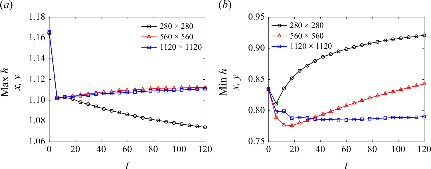
As for the accuracy test of our method, we perform a mesh-refinement study for the evolution of singular MQG modon. In figure 3, we show the results (
 $h$
) obtained on a coarser (
 $280\times 280$
) and finer (
 $1120\times 1120$
) meshes. As one can see, the solutions at a small time
 $t=6$
are very similar, but at larger times (
 $t=60$
and especially
 $t=120$
), they are only qualitatively similar since the locations of the computed modons are different: the modon propagates further towards the lower right corner of the computational domain when the mesh is refined. This is attributed to the fact that the large time modon propagation is affected by the amount of numerical diffusion, which also affects the magnitude of the modon; see figure 4. In fact, the lack of convergence, especially at large times, is typically observed when inviscid systems are studied numerically. In order to accurately capture both the position and amplitude of the modons, one has to add physical diffusion into the studied MRSW system and then to make sure that its affect is more significant than the affect of the numerical diffusion: this can be achieved by a mesh refinement, but obviously only in the case when the physical diffusion is not too small as otherwise an impractically fine mesh may be required to achieve the convergence. Studying viscous MRSW equations is, however, outside the scope of our manuscript.
The maximum (a) and minimum values of
 $h$
computed on three different meshes as function of time.

In order to investigate the late-stage dynamics of this phenomenon, we re-initialise our simulation at
 $t=120$
as follows. We take the obtained data on
 $2\leqslant x\leqslant 14$
and
 $-14\leqslant y\leqslant 14$
, extend them to the new computational domain
 $2\leqslant x\leqslant 30$
and
 $-14\leqslant y\leqslant 14$
by zero-order extrapolation from the
 $x=14$
to the
 $x\gt 14$
domain, set the free boundary conditions and then run the simulations for additional 400 time units. The time snapshots of the obtained
 $h$
,
 $b$
and
 $\zeta$
at
 $t=220$
,
 $320$
and
 $520$
are shown in figure 5. The evolution of the magnetic modon on the
 $f$
-plane demonstrates a significant transition from a quadrupole to a tripole magnetic field structure during the advanced stages of instability. This tripolar magnetic configuration is a transient state, as the magnetic field eventually reverts to the adjusted magnetic modon structure, as shown in figure 6, which shows the solution computed after another re-initialisation performed at
 $t=520$
. To this end, we took the solution at
 $t=520$
on
 $2\leqslant x\leqslant 30$
and
 $-14\leqslant y\leqslant 2$
, extended it to the new computational domain
 $2\leqslant x\leqslant 30$
and
 $-30\leqslant y\leqslant -2$
by zero-order extrapolation from the
 $y=-14$
to the
 $y\lt -14$
domain, set the free boundary conditions and then ran the simulations for additional
 $300$
time units. As the system undergoes clockwise rotation, the magnetic field reorganises into a tripolar configuration, characterised by a central negative core flanked by two positive satellites that orbit the core within a positively co-moving reference frame (
 $U\gt 0$
). Conversely, in a negatively co-moving reference frame (
 $U\lt 0$
), the configuration inverts, with two negative satellites rotating around a positive core; see figure 2. This emerging tripole structure is also subtly reflected in the vorticity field (figure 5, bottom row).
Further evolution of the singular MQG modon on the
 $f$
-plane after the re-initialisation. The panels, presented from the first to the third row, depict the evolution of
 $h$
overlaid with the velocity field,
 $b$
, and
 $\zeta$
. These quantities are illustrated at successive times
 $t=220$
, 320 and 520. The bottom row shows the corresponding time evolution of the total, mechanical and magnetic energies. Note that the colour bars have been adjusted compared with figure 2 for improved visibility.

Further evolution of the singular MQG modon to
 $t=820$
after the second re-initialisation. The sequence of panels displays
 $h$
overlaid with the velocity field,
 $b$
, and
 $\zeta$
. Note that the colour bars have been adjusted compared with figure 5 for improved visibility.

Same as in figure 1, but for a hollow MQG modon configuration with
 $\kappa _-=0$
,
 $\kappa _+=0.1$
and
 $U=0.1$
.

Same as in figure 1, but for a hollow modon configuration with
 $\kappa _-=0$
,
 $\kappa _+=0.1$
and negative co-moving frame velocity
 $U =-0.1$
.

3.2. Evolution of hollow MQG modon
In the presence of an external magnetic field positioned outside the separatrix radius, with no magnetic field inside the separatrix, a hollow modon is observed (see figure 7, top row). With parameter values
 $\kappa _-=0$
and
 $\kappa _+=0.1$
, the system exhibits a highly unstable configuration with an accelerated destabilisation rate compared with the previous scenario (figure 7, second to fourth rows). The onset of instability is characterised by vorticity anomalies near the separatrix, which propagate along and beyond this boundary, generating a wake on the lee side of the modon. For a positive (negative) co-moving frame velocity
 $U=0.1$
(
 $U=-0.1$
), the magnetic field displays distinct instability signatures on the eastern (western) flank of the eastward (westward) propagating modon. The resulting perturbation triggers secondary instabilities within the dipole, particularly at the saddle points where the modon axis intersects the outer separatrix. These instabilities are associated with nonlinear energy exchanges between the system’s mechanical and magnetic energy components, ultimately leading to the breakdown of the coherent modon structure (see figure 7, bottom row). The observed reduction in kinetic energy is linked to enhanced dissipation mechanisms, driven by the formation of small-scale filamentary structures as the instability progresses. This indicates that the form of dissipation in the numerical scheme affects the system’s detailed evolution. The qualitative evolution of instabilities remains consistent, with the destabilisation time scale altered only marginally by a few time units at most. Our results, in conjunction with the consistency observed in Lahaye & Zeitlin (Reference Lahaye and Zeitlin2022) despite differing numerical schemes, strongly validate that the small-scale instabilities and the modon destruction mechanism we observed are genuine physical phenomena, not numerical artefacts. The nonlinear evolution of a similar hollow MQG modon with negative co-moving frame velocity
 $U=-0.1$
is presented in figure 8.
3.3. Evolution of regular MQG modon
In order to examine the evolution of regular MQG modons, characterised by magnetic fields both inside and outside the separatrix circle on the
 $f$
-plane, we set the parameter values to
 $\kappa _-=0.1$
,
 $\kappa _+=0.1$
and
 $U=0.1$
(figure 9, top row). The nonlinear evolutions of regular and hollow MQG modons share several similarities. In both cases, the onset of instability is marked by vorticity anomalies near the separatrix, which propagate along and beyond this boundary, generating a wake on the lee side of the modon. However, the external domain outside the separatrix radius in the regular modon is broader compared with that of the hollow modon with similar
 $U$
and
 $\kappa _+$
parameters (figure 9, third row). Our results reveal that increased values of
 $\kappa _+$
enhance the instability of the dipolar magnetic structure. Specifically, hollow modons exhibit a faster onset of instability compared with regular modons, with a pronounced acceleration of instability development within the dipolar core. This accelerated instability in hollow modons is attributable to the tangential magnetic discontinuity arising from the disparity between
 $\kappa _-$
and
 $\kappa _+$
. The rapid temporal evolution of the magnetic field in hollow modons reflects this discontinuity, leading to more pronounced perturbations and an instability dynamics within the modon’s core region. The nonlinear evolution of a similar regular MQG modon with negative co-moving frame velocity
 $U=-0.1$
is presented in figure 10.
Same as in figure 1, but for a regular MQG modon configuration with
 $\kappa _-=0.1$
,
 $\kappa _+=0.1$
and
 $U=0.1$
.

Same as in figure 1, but for a regular modon configuration with
 $\kappa _-=0.1$
,
 $\kappa _+=0.1$
and negative co-moving frame velocity
 $U=-0.1$
.

Trajectories of the centres of three types of magnetic modons – singular (black circles), hollow (red triangles) and regular (blue squares) – on the
 $(x,y)$
-plane over a time span of
 $t=0-120$
, sampled at intervals of 6 time units. The trajectories are shown for co-moving frame velocities
 $U=0.1$
(a) and
 $U=-0.1$
(b).

Detailed spatial trajectories of the three types of magnetic modons – singular, hollow and regular – under positive and negative co-moving frame velocities are depicted in figure 11, which is determined by finding the midpoint position between the maximum and minimum values of
 $h$
. It illustrates that, up to approximately
 $t\approx 60$
, the magnetic modons maintain their coherence, propagating eastward for positive co-moving velocities and westward for negative co-moving velocities. However, as coherence diminishes and instabilities develop, the rate of southward (for positive
 $U$
) or northward (for negative
 $U$
) movement becomes roughly an order of magnitude greater than the eastward/westward movement. This increased deflection is primarily attributed to the Coriolis force, which exerts a stronger influence on the modons’ trajectories as instabilities grow. Notably, the hollow modon exhibits the most pronounced southward displacement, while the singular modon displays the least southward motion.
4. Collision of two magnetic modons in the MRSW model
In this section, we investigate the nonlinear dynamics governing the interactions between two MQG modons within the framework of the MRSW model. The study considers three principal scenarios for the initialisation of simulations: the collision of magnetic modons where the anticyclonic component of one modon collides with the cyclonic component of the other, and vice versa; the collision of magnetic modons with juxtaposed cyclonic components; and the collision of magnetic modons with juxtaposed anticyclonic components.
4.1. Collision of magnetic modons with opposing vortex components
Figure 12 depicts the interaction between two singular MQG modons, defined by the parameters
 $\kappa _-=0.1$
and
 $\kappa _+=0$
(see table 1), within the framework of the MRSW model. The modons are initialised in a co-moving reference frame with a zonal velocity
 $U=0.1$
for the left modon and
 $U=-0.1$
for the right one, which introduces a steady drift effect. As the system evolves, nonlinear interactions lead to the cyclonic vortex of the western modon dynamically coupling with the anticyclonic vortex of the eastern modon. This interaction triggers the emergence of a new composite modon structure that undergoes meridional bifurcation, where the coupled modon migrates northward, while the residual dipolar structure is advected southward. From an MHD perspective, this interaction precipitates the coalescence of two initially distinct positive magnetic poles, resulting in the formation of a singular, coherent positive magnetic pole that is flanked by two negative magnetic poles. This reorganisation of the magnetic field generates a novel magnetic tripole configuration, which exhibits a robust alignment with the emergent dipolar structure observable in both the isopycnal layer thickness (
 $h$
) and relative vorticity (
 $\zeta$
) fields. A similar tripolar magnetic structure is observed to form in the southern sector of the dipoles, propagating southward in tandem with the corresponding dipolar structure. Notably, while the vorticity field predominantly mirrors the spatial distribution of the isopycnal thickness, the late-stage dynamics reveals a subtle manifestation of the tripolar vorticity signature. This behaviour is indicative of the coupling between vorticity and magnetic field evolution, akin to the late-stage temporal dynamics observed in the evolution of an isolated singular modon (see figure 5).
First to third rows: time evolution of the MQG modons in the absence of an external magnetic field, showing the collision of juxtaposed opposite vortices. Parameter values are
 $\kappa _-=0.1$
,
 $\kappa _+=0$
and
 $U=0.1$
(
 $U=-0.1$
) for the left (right) modons. The panels, presented from top to bottom show the evolution of
 $h$
overlaid with the velocity field,
 $b$
, and
 $\zeta$
at times
 $t=0$
,
 $6$
,
 $60$
and
 $120$
. Bottom row: the corresponding time evolution of the total, mechanical and magnetic energies.

In the case of the regular modon collision scenario (see figure 13), a transition from mechanical to magnetic energy is observed, similar to the evolution of a single regular modon. This energy transfer leads to a more pronounced elliptical elongation of the central pole within the tripolar magnetic field.
Same as in figure 12, but for two regular MQG modons with both internal and external magnetic fields (inside and outside the separatrix), showing the collision of a cyclonic component from one modon with an anticyclonic component from the other, and vice versa.

4.2. Collision of magnetic modons with cyclonic components
Figure 14 captures the dynamical interaction between two singular MQG modons (see table 1) within the MRSW model, with particular emphasis on their collision via the cyclonic components. Upon interaction, the cyclonic vortices coalesce, leading to the formation of a tripolar structure. This newly formed tripole is characterised by a central cyclonic core with a pronounced negative layer thickness anomaly, flanked symmetrically by two anticyclonic poles. The entire tripolar system exhibits counterclockwise rotation, a motion governed by the distribution of relative vorticity and modulated by the planetary vorticity gradient of the Coriolis force effect. As the nonlinear evolution unfolds, the central vortex core undergoes a gradual deformation, transitioning from an initially circular to an elliptical shape. This morphological change is driven by the intensification of the surrounding satellite vortices. The differential rotation and the resultant shear forces exerted by these satellite vortices impose significant strain on the primary vortex core, culminating in its eventual bifurcation. The split core vortices, now paired with the intensified satellite vortices, reorganise into two distinct vortex dipoles that propagate along divergent paths, reflective of the inherent symmetry breaking. This process mirrors the barotropic dipole splitting typically observed in the nonlinear saturation phase of cyclonic instability, particularly under conditions where the most unstable azimuthal wavenumber is two, as highlighted in previous studies in Baey & Carton (Reference Baey and Carton2002); Rostami & Zeitlin (Reference Rostami and Zeitlin2017).
First to third rows: time evolution of the MQG modons in the absence of an external magnetic field, showing the collision of their cyclonic vortices. Parameter values are
 $\kappa _-=0.1$
,
 $\kappa _+=0$
and
 $U=0.1$
(
 $U=-0.1$
) for the left (right) modons. The panels, presented from top to bottom show the evolution of
 $h$
overlaid with the velocity field,
 $b$
, and
 $\zeta$
at times
 $t=0$
,
 $6$
,
 $60$
and
 $120$
. Bottom row: the corresponding time evolution of the total, mechanical and magnetic energies.

The vorticity field, which is tightly coupled to the layer thickness distribution, also manifests as a dipolar structure. In the advanced stages of the instability, the vorticity field reveals a subtle yet discernible tripolar signature, underscoring the intricate interplay between the large-scale flow and smaller-scale coherent structures. This emergent tripolar vorticity pattern is indicative of a vortex dynamics that reflects the redistribution of enstrophy within the flow field.
Simultaneously, the magnetic field evolution gives rise to perturbed tripole structures that coexist and propagate with the emerging fluid dipoles. These MHD tripoles are characterised by a central negative magnetic pole, flanked by oppositely charged magnetic poles, collectively mirroring the dynamics of the fluid flow. The evolution of these magnetic tripoles is closely linked to the underlying fluid motions, demonstrating the strong coupling between magnetic fields and the fluid dynamics within the MRSW model.
First to third rows: time evolution of the MQG modons in the absence of an external magnetic field, showing the collision of their anticyclonic vortices. Parameter values are
 $\kappa _-=0.1$
,
 $\kappa _+=0$
and
 $U=0.1$
(
 $U =-0.1$
) for the left (right) modons. The panels, presented from top to bottom show the evolution of
 $h$
overlaid with the velocity field,
 $b$
, and
 $\zeta$
at times
 $t=0$
,
 $6$
,
 $60$
and
 $120$
. Bottom row: the corresponding time evolution of the total, mechanical and magnetic energies.

4.3. Collision of magnetic modons with anticyclonic components
Figure 15 illustrates the nonlinear evolution of two singular MQG modons (see table 1) within the MRSW model, focusing on their interaction through anticyclonic components. Similar to the cyclonic interaction discussed in §§ 4.2, the anticyclonic vortices coalesce, forming a tripolar structure characterised by a dominant central anticyclone flanked by two cyclonic satellite vortices. This tripolar configuration exhibits a clockwise rotation, driven by the underlying vorticity distribution and modulated by the planetary vorticity gradient.
A key distinction between this scenario and the cyclonic collision is the enhanced structural stability of the tripolar configuration. Unlike the cyclonic collision case, where barotropic dipole splitting occurs, the tripolar structure formed through anticyclonic interaction demonstrates remarkable resilience, maintaining its coherence. The persistence of this structure is strongly evident in both
 $h$
and
 $\zeta$
, indicating a robust coupling between the large-scale flow and the coherent vortex structures.
Regarding the evolution of the magnetic field, the system exhibits pronounced instability, as evidenced by the development of small-scale meso- and sub-mesoscale localised magnetic fields. These localised fields contribute to an elevated dissipation rate and a significant loss of magnetic energy, thereby emphasising the interplay between the fluid dynamics and the magnetic field evolution within the MRSW model framework.
Same as in figure 15, but for two regular MQG modons with both internal and external magnetic fields (inside and outside the separatrix), showing the collision of their anticyclonic components.

Figure 16 illustrates the collision of two regular MQG modons, characterised by the presence of magnetic field structures both inside and outside the separatrix. The interaction of their anticyclonic components leads to the emergence of a stationary tripolar structure, consisting of a central anticyclonic vortex flanked by two oppositely rotating cyclonic vortices. This tripolar configuration is clearly visible in the layer thickness and vorticity fields during the evolution; see figure 16.
Unlike freely propagating modons, this tripolar structure does not exhibit independent translational motion; instead, it remains quasi-stationary and is advected by the ambient plasma flow. Similar tripolar structures have been identified in previous studies as nonlinear equilibrium solutions of the governing equations of plasma dynamics, particularly in the context of linear shear flow and non-uniform dust density distributions (Vranješ et al. Reference Vranješ, Petrović and Shukla2001). These structures have been shown to act as transport barriers, influencing the confinement and mixing of plasma particles.
A notable aspect of this collision event is the self-organisation of the initially chaotic magnetic field generated by the interaction. As the system evolves, the disordered magnetic field realigns into a structured chain of alternating positive and negative magnetic poles, forming a checkered-like pattern. This organisation process leads to a stationary chain of magnetic dipoles, with their amplitude gradually diminishing as the radial distance from the central anticyclonic vortex increases. This checkered magnetic pattern becomes particularly prominent during the later stages of the collision; see figure 16, right panel of magnetic field. The formation of these coherent tripolar structures and the subsequent emergence of ordered magnetic field patterns highlight the robustness of such interactions in governing the evolution of magnetised modons.
4.4. Role of slow and fast magneto-inertia-gravity waves
Our key observations of dynamical processes associated with slow and fast magneto-inertia-gravity (MIG) waves reveal that the coalescence of opposite vortex components redistributes energy between mechanical and magnetic forms. The formation of a tripolar magnetic structure and its subsequent alignment with dipolar vorticity patterns are accompanied by the excitation of slow MIG waves, strongly influenced by magnetic field reorganisation.
In singular modon interactions, the reconfiguration of magnetic poles generates new coherent structures, implying the presence of a slow MIG wave dynamics dominated by magnetic tension and vorticity interactions. Conversely, in regular modon collisions, the transition from mechanical to magnetic energy excites fast MIG waves, where inertial and gravitational effects play a more significant role.
The north-south splitting of modons and the emergence of distinct propagating structures exhibit characteristics of slow MIG waves, typically associated with barotropic instability in MHD fluids. The elliptical elongation of structures during the nonlinear evolution phase suggests mixed-mode interactions, where both fast and slow MIG waves contribute to deformation.
Overall, slow MIG waves govern the long-term evolution of coherent structures via vorticity–magnetic field coupling, whereas fast MIG waves facilitate transient energy exchanges and structural deformation during early interaction stages.
5. Conclusion
We investigate the nonlinear evolution of MQG modons within the
 $f$
-plane approximation using the MRSW model, focusing on different magnetic field configurations and their effects. The simulations incorporate three classes of magnetic modons, namely, singular, hollow and regular modons based on the distribution of the magnetic field within and outside the modon core. All of the numerical experiments have been conducted using the second-order locally divergence-free well-balanced path-conservative central-upwind scheme.
For singular MQG modons, where the magnetic field is confined to the core, the modon displays a coherent dipolar structure and propagates either eastward or westward depending on the co-moving velocity. In the later stages of instability, it transitions to a transient tripolar structure before ultimately reverting to its coherent adjusted magnetic modon configuration, which embodies a quadruple magnetic field pattern. Hollow MQG modons, characterised by an external magnetic field and no internal field, display rapid destabilisation. Instabilities develop near the separatrix and propagate, leading to breakdown of the modon structure and accelerated energy dissipation. Regular MQG modons, with magnetic fields inside and outside the core, exhibit a similar onset of instability as hollow modons. However, instability progresses more slowly compared with hollow modons, due to the broader external magnetic domain and less pronounced tangential discontinuities. The findings highlight that hollow modons are more susceptible to rapid destabilisation compared with regular modons, with the instability dynamics influenced by the magnetic field configuration and co-moving velocity.
The trajectories of the three magnetic modon types show distinct behaviours under positive and negative co-moving frame velocities. Initially, modons maintain coherence with eastward propagation for positive velocities and westward for negative velocities. As instabilities increase, the southward or northward deflection becomes significantly larger than the eastward or westward movement, primarily due to the influence of the Coriolis force. Among them, the hollow modon exhibits the most substantial southward displacement, while the singular modon shows the least.
In examining the nonlinear dynamics of modon collisions, three primary scenarios were investigated: the first scenario involves collisions where the cyclonic component of one modon meets the anticyclonic component of another one. This interaction leads to the formation of a new composite modon structure, characterised by a central positive magnetic pole surrounded by two negative poles. As a result, the system experiences a meridional bifurcation, with the newly formed modon migrating poleward while the residual dipole moves equatorward. In the second scenario, when two cyclonic vortices collide, they coalesce into a tripolar structure with a central cyclonic core and two anticyclonic poles on either side. This tripole exhibits counterclockwise rotation and undergoes a transition from a circular to an elliptical shape due to the influence of surrounding satellite vortices. The primary vortex core eventually bifurcates, resulting in two distinct vortex dipoles that propagate along diverging paths. The vorticity field in this case shows a subtle tripolar signature, reflecting the redistribution of enstrophy within the flow. The third scenario involves collisions between anticyclonic components, leading to the formation of a tripolar structure with a central anticyclone and two cyclonic satellite vortices. This configuration is notably more stable than the cyclonic interaction case and maintains its coherence longer. The magnetic field evolves into a checkered pattern of alternating magnetic poles. During the later stages of the collision, particularly for regular modons, this pattern becomes more pronounced.
The emergence of the quasi-stationary checkered magnetic field and tripolar vortex patterns can be attributed to the reorganisation of Alfvénic perturbations, which align with the induced vorticity field and mitigate large-scale distortions. The tripolar structure demonstrates enhanced stability, as its stationary nature minimises advective deformations, enabling sustained coherence over extended time scales. Furthermore, the formation of this coherent structure imposes constraints on cross-field plasma transport, leading to localised confinement regions within the magnetised flow.
Funding
The work of Y.C. was supported in part by the Guangdong Basic and Applied Basic Research Foundation (No. 2025A1515012249). The work of A.K. was supported in part by NSFC grants 12171226 and W2431004. M.R. is grateful to Virgin Unite USA, Inc. through the Planetary Boundary Science Lab.
Declaration of interests
The authors report no conflict of interest.
Appendix A. Derivation of Magnetic Modon Solutions
Following Lahaye & Zeitlin (Reference Lahaye and Zeitlin2022), we revisit the derivation of a localised, stationary solution in a reference frame moving with a constant velocity
 $U\hat {\boldsymbol{x}}$
(co-moving frame). In this frame, the streamfunction
 $\psi$
and the magnetic potential
 $A$
take the forms
 $\psi =\psi (x-Ut,y)$
and
 $A=A(x-Ut,y)$
, respectively. Under these conditions, the MQG system (2.10)–(2.11) transforms into the following form:
 \begin{align}& -Uq_x+{\mathcal J}(\psi ,q)-{\mathcal J}(A,\nabla ^2A)=0, \end{align}
 \begin{align}&\qquad\quad -UA_x+{\mathcal J}(\psi ,A)=0. \end{align}
Equation (A2) implies that
 ${\mathcal J}(\psi +Uy,A)=0$
, leading to the relation
 $A=F(\psi +Uy)$
, where
 $F$
is an arbitrary function. For simplicity, we assume a linear relationship
 \begin{equation} A=\kappa (\psi +Uy), \end{equation}
where
 $\kappa$
is a constant that quantifies the proportionality between the magnetic potential and the streamfunction
 $\psi$
in the co-moving frame. Substituting (A3) into (A1) results in
 \begin{equation} {\mathcal J}(\psi +Uy,q)-{\mathcal J}(A,\nabla ^2A)=0. \end{equation}
Given (A3), the Jacobian
 ${\mathcal J}(A,\nabla ^2A)$
can be expressed as
 \begin{equation} {\mathcal J}(A,\nabla ^2A)=\kappa ^2{\mathcal J}(\psi +Uy,\nabla ^2\psi ), \end{equation}
which simplifies the PV equation to
 \begin{equation} {\mathcal J}\left (\psi +Uy,(1-\kappa ^2)\nabla ^2\psi -\psi \right )=0. \end{equation}
This equation suggests that
 \begin{equation} (1-\kappa ^2)\nabla ^2\psi -\psi =G(\psi +Uy), \end{equation}
where
 $G$
is another arbitrary function. We assume
 $G(x)=\alpha x$
, with
 $\alpha$
being a constant. This choice is analogous to the classical modon solutions derived in Larichev & Reznik (Reference Larichev and Reznik1976), where
 $\alpha$
characterises the PV anomaly strength relative to the streamfunction in the co-moving frame.
Adopting the classical approach, we divide the domain into inner (
 $-$
) and outer (
 $+$
) regions, separated by a circular separatrix of radius
 $r=\sqrt {x^2+y^2}=r_0$
. The constants
 $\alpha$
and
 $\kappa$
are allowed to differ between these regions, denoted as
 $\alpha _\pm$
and
 $\kappa _\pm$
, respectively. Consequently, the streamfunctions
 $\psi _\pm$
satisfy the following equations in the outer and inner regions:
 \begin{equation} (1-\kappa ^2_\pm )\nabla ^2\psi _\pm -\psi _\pm =\alpha _\pm (\psi _\pm +Uy). \end{equation}
These solutions must satisfy the boundary conditions that ensure the continuity of velocity and pressure across the separatrix.
A.1.
Solution in the outer region
 $r\gg r_0$

We seek a localised solution with finite energy, as defined by the energy functional in (2.12), which vanishes asymptotically as
 $r\to \infty$
. This requirement imposes
 $\alpha _+=0$
, leading to the simplified linear equation
 \begin{equation} (1-\kappa ^2_+)\nabla ^2\psi _+-\psi _+=0. \end{equation}
A decaying solution for large
 $r$
can be obtained by separating variables in polar coordinates
 $(r,\theta )$
. Considering that matching with the inner solution is performed in the co-moving frame, where a constant zonal velocity corresponds to a streamfunction linear in
 $y=r\sin \theta$
, we obtain
 \begin{equation} \psi _+=C_+K_1\left (\frac {r}{\sqrt {1-\kappa ^2_+}}\right )\sin \theta , \end{equation}
where
 $K_1$
is the modified Bessel function of the second kind. Notably, this decaying solution exists only if
 $1-\kappa ^2_+\gt 0$
. The specific case
 $\kappa _+=0$
indicates that the magnetic field is confined to the inner region, while
 $\kappa _+\ne 0$
corresponds a constant background zonal magnetic field
 $B=-A_y=-\kappa _+U$
permeating the entire domain, consistent with (A3).
A.2.
Solution in the inner region
$r\ll r_0$

In the inner region, the governing equation becomes
 \begin{equation} \left(1-\kappa ^2_- \right)\nabla ^2\psi _{-}-\psi_{-}=\alpha _-\left(\psi _-+Uy \right), \end{equation}
whose general solution comprises a homogeneous solution
 $\psi _h$
and a particular solution
 $\psi _p$
satisfying
 \begin{equation} \left(1-\kappa ^2_- \right)\nabla ^2\psi _h-\left(1+\alpha _- \right)\psi _h=0, \end{equation}
and
 \begin{equation} \psi _p=-\frac {\alpha _-Uy}{1+\alpha _-}, \end{equation}
respectively. Assuming the same angular structure to ensure smooth matching with the outer solution, the inner streamfunction is expressed as
 \begin{equation} \psi _-=\left (C_-J_1(\lambda r)-\frac {\alpha _-Ur}{1+\alpha _-}\right )\sin \theta , \end{equation}
where
 $J_1$
is the Bessel function of the first kind, and
 $\lambda ^2=-{1+\alpha _-}/{1-\kappa ^2_-}$
. It is important to note the presence of a singularity at
 $\kappa _- = 1$
.
A.3. Matching conditions
The streamfunctions must be matched across the separatrix to ensure the continuity of the co-moving streamfunction, yielding the smoothest possible solution
 \begin{equation} (\psi _++Uy)\left |_{r=r_0}=(\psi _-+Uy)\right |_{r=r_0}=0. \end{equation}
This continuity condition allows us to determine the constants
 $C_\pm$
as follows:
 \begin{equation} C_+=-\frac {Ur_0}{K_1\left (\dfrac {r_0}{\sqrt {1-\kappa _+}}\right )},\quad C_-=-\frac {Ur_0}{(1+\alpha _-)J_1(\lambda r_0)}. \end{equation}
The magnitude of the modon, characterised by the streamfunction, is primarily governed by
 $Ur_0$
and modulated by
 $\alpha _-$
. However,
 $\alpha _-$
is not an arbitrary parameter but is instead determined by the matching conditions, which also influence the radial structure of the streamfunction through
 $\lambda$
.
Enforcing the continuity of the radial derivative of the streamfunction,
 $(\psi _+)_r=(\psi _-)_r$
at
 $r=r_0$
, results in the following transcendental equation for the eigenvalues
 $\lambda$
given
 $r_0$
and
 $\kappa _+$
, and consequently for
 $\alpha _-$
given
 $\kappa _-$
:
 \begin{equation} \frac {C_+}{\sqrt {1-\kappa ^2_+}}K_1'\left (\frac {r_0}{\sqrt {1-\kappa ^2_+}}\right )=C_-\lambda J_1'(\lambda r_0)-\frac {\alpha _-U}{1+\alpha _-}, \end{equation}
where
 $C_\pm$
are defined in (A16), and the prime denotes differentiation with respect to the argument.