2 Formulation for the inertial drift: the generalized reciprocal theorem

The velocity and stress fields in two different problems, the problem of interest and a test problem, corresponding to two different flow configurations past the same particle, can be related through a generalized reciprocal theorem (Leal Reference Leal1979; Subramanian & Koch Reference Subramanian and Koch2005, Reference Subramanian and Koch2006b ; Einarsson et al. Reference Einarsson, Candelier, Lundell, Angilella and Mehlig2015; Dabade et al. Reference Dabade, Marath and Subramanian2016). The two problems are defined based on a dynamical quantity that needs to be evaluated for the problem of interest. The test problem is usually chosen to be one in which the velocity and stress fields are known a priori. In the present case, the quantity of interest is the correction to the angular velocity of a neutrally buoyant spheroid suspended in a Newtonian fluid undergoing a planar linear flow, with the inertial acceleration, both that of the particle and that of the fluid, being taken into account. The disturbance velocity and stress fields in the aforementioned problem of interest are denoted by $\boldsymbol{u}^{\prime (1)}$ and $\unicode[STIX]{x1D748}^{\prime (1)}$ . The disturbance fields are related to the total velocity and stress fields in the problem by $\boldsymbol{u}^{\prime (1)}=\boldsymbol{u}^{(1)}-\unicode[STIX]{x1D71E}\boldsymbol{\cdot }\boldsymbol{x}$ and $\unicode[STIX]{x1D748}^{\prime (1)}=\unicode[STIX]{x1D748}^{(1)}-\unicode[STIX]{x1D748}^{(\infty )}=\unicode[STIX]{x1D748}^{(1)}+p^{\infty }\unicode[STIX]{x1D644}-2\unicode[STIX]{x1D640}$ . Here, $\unicode[STIX]{x1D71E}\boldsymbol{\cdot }\boldsymbol{x}$ is the ambient planar linear flow in non-dimensional form defined with the origin at the centre of the spheroid. The transpose of the non-dimensional (ambient) velocity gradient tensor and the rate-of-strain tensor, in a space-fixed coordinate system ( $X^{\prime }Y^{\prime }Z^{\prime }$ , with the unit vector triplet $\mathbf{1}_{x}^{\prime },\mathbf{1}_{y}^{\prime }$ and $\mathbf{1}_{z}^{\prime }$ ), are given by $\unicode[STIX]{x1D71E}=\mathbf{1}_{x}^{\prime }\mathbf{1}_{y}^{\prime }+\unicode[STIX]{x1D706}\mathbf{1}_{y}^{\prime }\mathbf{1}_{x}^{\prime }$ and $\unicode[STIX]{x1D640}=(\mathbf{1}_{x}^{\prime }\mathbf{1}_{y}^{\prime }+\mathbf{1}_{y}^{\prime }\mathbf{1}_{x}^{\prime })(\unicode[STIX]{x1D706}+1)/2$ respectively. 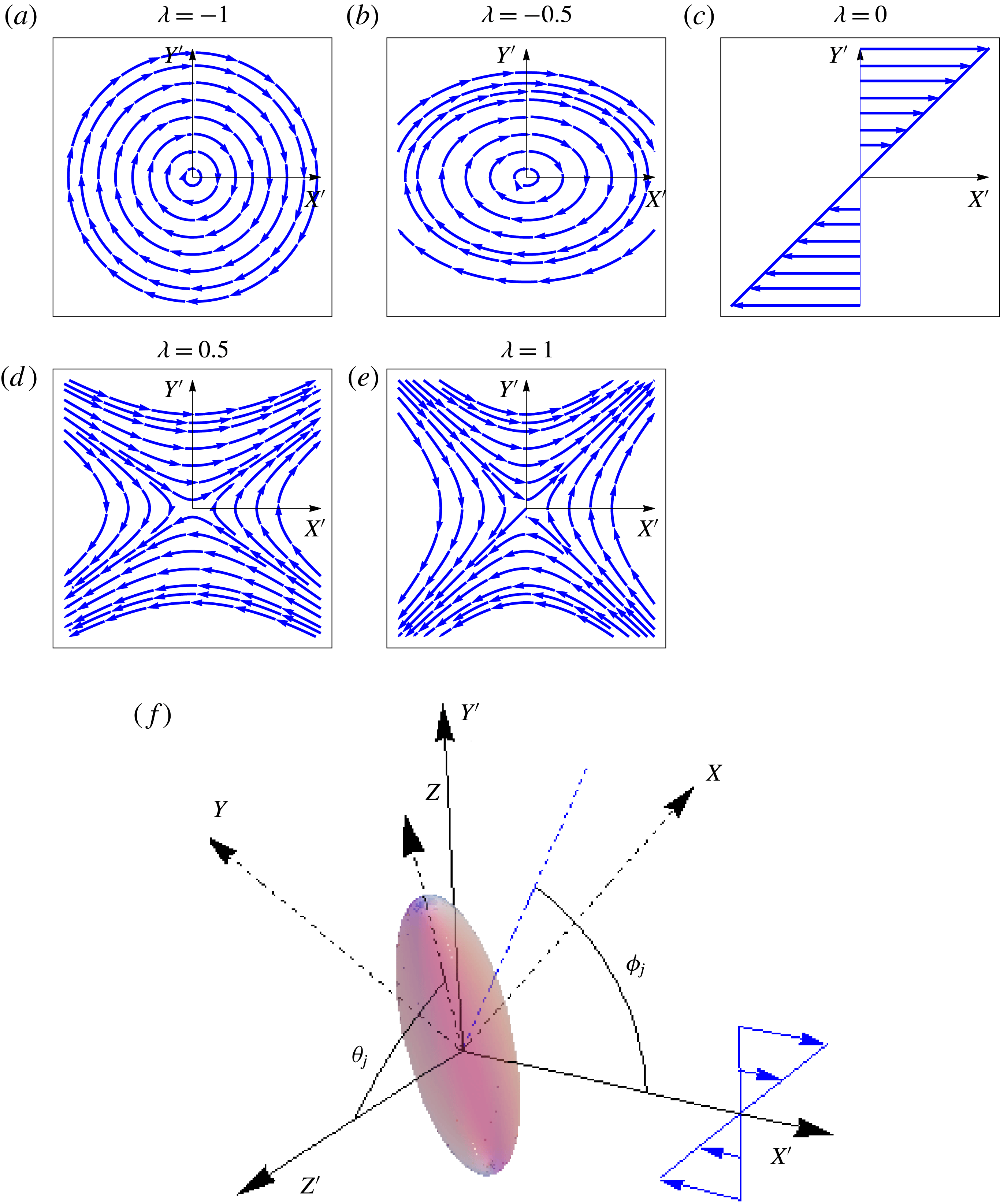As mentioned earlier, the parameter $\unicode[STIX]{x1D706}$ characterizes the family of planar linear flows, with $(1-\unicode[STIX]{x1D706})/(1+\unicode[STIX]{x1D706})$ denoting the rate of vorticity to extension in the flow. The ambient streamline patterns for these flows are shown in figure 1. As $\unicode[STIX]{x1D706}$ increases from $-1$ to 1, there is a transition from a closed (figure 1 a,b) to an open streamline pattern (figure 1 d,e), with the streamlines for $\unicode[STIX]{x1D706}=0$ alone (figure 1 c) being straight lines. The axes of the space-fixed coordinate system, $X^{\prime }$ , $Y^{\prime }$ and $Z^{\prime }$ , are defined such that they coincide with the flow, the gradient and the vorticity directions of the simple shear flow ( $\unicode[STIX]{x1D706}=0$ ) respectively (figure 1 f). The ambient pressure ( $p^{\infty }$ ) required to maintain the linear flow for finite $Re$ is obtained by equating its gradient to the inertial acceleration, whence one finds $p^{\infty }=-Re\,\boldsymbol{x}\boldsymbol{\cdot }\unicode[STIX]{x1D71E}\boldsymbol{\cdot }\unicode[STIX]{x1D71E}\boldsymbol{\cdot }\boldsymbol{x}/2$ . It should be noted that $p^{\infty }=0$ for simple shear flow.

Figure 1.

The ambient streamline patterns in the spaced-fixed coordinate system for (a) solid-body rotation, (b) elliptic linear flow, (c) simple shear flow, (d) hyperbolic linear flow and (e) planar extensional flow. In (f), the body-aligned and space-fixed coordinate systems are shown for a spheroid in simple shear flow.

The test problem, with its velocity and stress fields denoted by $\boldsymbol{u}^{(2)}$ and $\unicode[STIX]{x1D748}^{(2)}$ respectively, corresponds to the Stokesian rotation of a spheroid in an otherwise quiescent ambient, with the same instantaneous orientation as that in the problem of interest. We also define two second-order tensors $\unicode[STIX]{x1D647}_{2}$ , $\unicode[STIX]{x1D650}^{(2)}$ and a third-order tensor $\unicode[STIX]{x1D72E}^{(2)}$ , which relate $\boldsymbol{{\mathcal{L}}}_{2}$ (the torque acting on the spheroid in the test problem), $\boldsymbol{u}^{(2)}$ and $\unicode[STIX]{x1D748}^{(2)}$ respectively to $\unicode[STIX]{x1D734}_{2}$ (the angular velocity in the test problem), the relations being given by $\boldsymbol{{\mathcal{L}}}_{2}=\unicode[STIX]{x1D647}_{2}\boldsymbol{\cdot }\unicode[STIX]{x1D734}_{2}$ , $\boldsymbol{u}^{(2)}=\unicode[STIX]{x1D650}^{(2)}\boldsymbol{\cdot }\unicode[STIX]{x1D734}_{2}$ and $\unicode[STIX]{x1D748}^{(2)}=\unicode[STIX]{x1D72E}^{(2)}\boldsymbol{\cdot }\unicode[STIX]{x1D734}_{2}$ . The expressions for these tensors are given in §§ 3 and 4 (alternatively, see Dabade et al. Reference Dabade, Marath and Subramanian2016).

The derivation of the reciprocal theorem, which gives the inertial correction to the angular velocity in the problem of interest ( $\unicode[STIX]{x1D734}_{1}$ ), is similar to that for a spheroid in a Newtonian fluid undergoing simple shear flow given in § 2 of Dabade et al. (Reference Dabade, Marath and Subramanian2016), except for an additional contribution that comes from the ambient pressure field. Here, we only present the final result and the reader is referred to Dabade et al. (Reference Dabade, Marath and Subramanian2016) for the details,

(2.1) $$\begin{eqnarray}\displaystyle \unicode[STIX]{x1D734}_{1}\boldsymbol{\cdot }\unicode[STIX]{x1D647}_{2} & = & \displaystyle \unicode[STIX]{x1D71E}:\int _{S_{p}}\boldsymbol{x}(\unicode[STIX]{x1D72E}^{(2)}\boldsymbol{\cdot }\boldsymbol{n})\,\text{d}S+St\,\frac{\text{d}}{\text{d}t}({\unicode[STIX]{x1D644}_{p}\boldsymbol{\cdot }\unicode[STIX]{x1D734}}_{1})+Re\int _{V}\left[\frac{\unicode[STIX]{x2202}\boldsymbol{u}^{\prime (1)}}{\unicode[STIX]{x2202}t}+(\unicode[STIX]{x1D71E}\boldsymbol{\cdot }\boldsymbol{x})\boldsymbol{\cdot }\unicode[STIX]{x1D735}\boldsymbol{u}^{\prime (1)}\right.\nonumber\\ \displaystyle & & \displaystyle \left.+\,\unicode[STIX]{x1D71E}\boldsymbol{\cdot }\boldsymbol{u}^{\prime (1)}+\boldsymbol{u}^{\prime (1)}\boldsymbol{\cdot }\unicode[STIX]{x1D735}\boldsymbol{u}^{\prime (1)}+\unicode[STIX]{x1D734}_{b}\wedge \boldsymbol{u}^{\prime (1)}-(\unicode[STIX]{x1D734}_{b}\wedge \boldsymbol{x}).\unicode[STIX]{x1D735}\boldsymbol{u}^{\prime (1)}\right]\boldsymbol{\cdot }\unicode[STIX]{x1D650}^{(2)}\,\text{d}V\nonumber\\ \displaystyle & & \displaystyle -\,Re\,\int _{S_{p}}\frac{\boldsymbol{x}\boldsymbol{\cdot }\unicode[STIX]{x1D71E}\boldsymbol{\cdot }\unicode[STIX]{x1D71E}\boldsymbol{\cdot }\boldsymbol{x}}{2}(\boldsymbol{x}\wedge \boldsymbol{n})\,\text{d}A.\end{eqnarray}$$

The reciprocal theorem above may also be seen in Candelier et al. (Reference Candelier, Einarsson, Lundell, Mehlig and Angilella2015a ). The authors did not evaluate the ambient pressure contribution correctly, which was rectified in a later communication (Candelier et al. Reference Candelier, Einarsson, Lundell, Mehlig and Angilella2015b ). The surface integrals in (2.1) are over the spheroid ( $S_{p}$ ) and the volume integral is over the unbounded fluid outside the spheroid ( $V$ ). In (2.1), $\unicode[STIX]{x1D644}_{p}$ is the moment of inertia tensor of the spheroid, given by $(4\unicode[STIX]{x03C0}/15)\bar{\unicode[STIX]{x1D709}}_{0}^{2}[(2\bar{\unicode[STIX]{x1D709}}_{0}^{2}/\unicode[STIX]{x1D709}_{0}^{4})\boldsymbol{p}\boldsymbol{p}+((2\unicode[STIX]{x1D709}_{0}^{2}-1)/\unicode[STIX]{x1D709}_{0}^{4})(\unicode[STIX]{x1D644}-\boldsymbol{p}\boldsymbol{p})]$ and $(4\unicode[STIX]{x03C0}/15)\bar{\unicode[STIX]{x1D709}}_{0}[(2/\unicode[STIX]{x1D709}_{0})\boldsymbol{p}\boldsymbol{p}+$ $((2\unicode[STIX]{x1D709}_{0}^{2}-1)/\unicode[STIX]{x1D709}_{0}^{3})(\unicode[STIX]{x1D644}-\boldsymbol{p}\boldsymbol{p})]$ for prolate and oblate spheroids respectively. Here, $\boldsymbol{p}$ is the spheroid orientation vector and $\unicode[STIX]{x1D709}_{0}$ is the inverse of the spheroid eccentricity.

As shown by Dabade et al. (Reference Dabade, Marath and Subramanian2016) and later in § 3, the disturbance velocity field around a spheroid in Stokes flow is expressed in a body-aligned spheroidal coordinate system. Therefore, while deriving (2.1), we transformed the reciprocal theorem from the original space-fixed coordinate system ( $X^{\prime }Y^{\prime }Z^{\prime }$ in figure 1 f) to a body-aligned coordinate system ( $XYZ$ in figure 1 f; see Dabade et al. Reference Dabade, Marath and Subramanian2016). The angles $\unicode[STIX]{x1D703}_{j}$ and $\unicode[STIX]{x1D719}_{j}$ determine the orientation of the spheroid (the $Z$ axis) with respect to the space-fixed coordinate system. To simplify the calculation, we restrict the $Y$ axis of the body-aligned coordinate system to the flow-gradient plane. This restriction makes the angular velocity of the body-aligned coordinate system, denoted by $\unicode[STIX]{x1D734}_{b}$ in (2.1), different from $\unicode[STIX]{x1D734}_{1}$ . The unit vectors of the body-aligned coordinate system $XYZ$ can be expressed in terms of those of the space-fixed coordinate system $X^{\prime }Y^{\prime }Z^{\prime }$ (see figure 1) as $\mathbf{1}_{x}=\cos \unicode[STIX]{x1D703}_{j}\cos \unicode[STIX]{x1D719}_{j}\mathbf{1}_{x}^{\prime }+\cos \unicode[STIX]{x1D703}_{j}\sin \unicode[STIX]{x1D719}_{j}\mathbf{1}_{y}^{\prime }-\sin \unicode[STIX]{x1D703}_{j}\mathbf{1}_{z}^{\prime },\mathbf{1}_{y}=-\sin \unicode[STIX]{x1D719}_{j}\mathbf{1}_{x}^{\prime }+\cos \unicode[STIX]{x1D719}_{j}\mathbf{1}_{y}^{\prime }$ and $\mathbf{1}_{z}=\sin \unicode[STIX]{x1D703}_{j}\cos \unicode[STIX]{x1D719}_{j}\mathbf{1}_{x}^{\prime }+\sin \unicode[STIX]{x1D703}_{j}\sin \unicode[STIX]{x1D719}_{j}\mathbf{1}_{y}^{\prime }+\cos \unicode[STIX]{x1D703}_{j}\mathbf{1}_{z}^{\prime }$ .

Although (2.1) is valid for arbitrary $Re$ , it is only of limited use in this general form because $\boldsymbol{u}^{\prime (1)}$ is not known for finite $Re$ . We therefore analyse (2.1) in the limit of $Re$ being small but finite, and determine $\unicode[STIX]{x1D734}_{1}$ to $O(Re)$ . The leading-order angular velocity ( $\unicode[STIX]{x1D734}_{jeff}$ ) corresponding to the Stokes regime can be obtained by equating the left-hand side of (2.1) to the first term on its right-hand side. The subscript ‘ $jeff$ ’ is used for the leading-order angular velocity since $\unicode[STIX]{x1D734}_{jeff}$ leads to closed orbits for a certain subset of planar linear flows (those with vorticity above an aspect-ratio-dependent threshold), which are identified in § 4. These are again spherical ellipses, as in simple shear, and are also termed as Jeffery orbits. The leading-order angular velocity is defined in the body-aligned coordinate system in terms of $\dot{\unicode[STIX]{x1D719}}_{j}$ and $\dot{\unicode[STIX]{x1D703}}_{j}$ as $\unicode[STIX]{x1D734}_{jeff}=-\dot{\unicode[STIX]{x1D719}}_{j}\sin \unicode[STIX]{x1D703}_{j}\,\mathbf{1}_{x}+\dot{\unicode[STIX]{x1D703}}_{j}\,\mathbf{1}_{y}-\cos \unicode[STIX]{x1D703}_{j}(1-\unicode[STIX]{x1D706})/2\,\mathbf{1}_{z}$ , where $\dot{\unicode[STIX]{x1D719}}_{j}$ and $\dot{\unicode[STIX]{x1D703}}_{j}$ are given by (Hinch & Leal Reference Hinch and Leal1972)

(2.2) $$\begin{eqnarray}\displaystyle & \displaystyle \dot{\unicode[STIX]{x1D719}}_{j}=-\!\left(\frac{1-\unicode[STIX]{x1D706}}{2}\right)+\left(\frac{1+\unicode[STIX]{x1D706}}{2}\right)\frac{\unicode[STIX]{x1D705}^{2}-1}{\unicode[STIX]{x1D705}^{2}+1}\cos 2\unicode[STIX]{x1D719}_{j}, & \displaystyle\end{eqnarray}$$

(2.3) $$\begin{eqnarray}\displaystyle & \displaystyle \dot{\unicode[STIX]{x1D703}_{j}}=\left(\frac{1+\unicode[STIX]{x1D706}}{4}\right)\frac{\unicode[STIX]{x1D705}^{2}-1}{\unicode[STIX]{x1D705}^{2}+1}\sin 2\unicode[STIX]{x1D703}_{j}\sin 2\unicode[STIX]{x1D719}_{j}, & \displaystyle\end{eqnarray}$$

with $b$ as the minor axis of the spheroid, $\unicode[STIX]{x1D705}=L/b~(b/L)$ for a prolate (an oblate) spheroid. The inertial contributions to $\unicode[STIX]{x1D734}_{1}$ in (2.1) include that due to the particle (the term proportional to $St$ ) and the fluid inertial contributions (the terms proportional to $Re$ ) on the right-hand side of (2.1). The last term proportional to $Re$ is due to the non-trivial ambient pressure field and may be interpreted as a centrifugal buoyancy. For simple shear flow, this contribution is zero, and (2.1) reduces to (2.21) in Dabade et al. (Reference Dabade, Marath and Subramanian2016).

The $O(Re)$ and $O(St)$ corrections to the angular velocity can be obtained by replacing $\boldsymbol{u}^{\prime (1)}$ with $\boldsymbol{u}_{s}^{\prime (1)}$ , the Stokes disturbance velocity field for a spheroid in a planar linear flow, $\unicode[STIX]{x1D734}_{\mathbf{1}}$ with $\unicode[STIX]{x1D734}_{jeff}$ in the term proportional to $St$ , and $\unicode[STIX]{x1D734}_{\boldsymbol{b}}$ with $\unicode[STIX]{x1D734}_{jeff}^{t}$ on the right-hand side of (2.1). The leading-order angular velocity of the body-aligned coordinate system, $\unicode[STIX]{x1D734}_{jeff}^{t}$ , differs from $\unicode[STIX]{x1D734}_{jeff}$ in the spin component, due to the restriction on the $Y$ axis of the body-aligned coordinate system discussed above; $\unicode[STIX]{x1D734}_{jeff}^{t}=-\dot{\unicode[STIX]{x1D719}}_{j}\sin \unicode[STIX]{x1D703}_{j}\mathbf{1}_{x}+\dot{\unicode[STIX]{x1D703}}_{j}\mathbf{1}_{y}+\dot{\unicode[STIX]{x1D719}}_{j}\cos \unicode[STIX]{x1D703}_{j}\mathbf{1}_{z}$ . Thus, to $O(Re)$ , (2.1) becomes

(2.4) $$\begin{eqnarray}\displaystyle \unicode[STIX]{x1D734}_{1}\boldsymbol{\cdot }\unicode[STIX]{x1D647}_{2} & = & \displaystyle \unicode[STIX]{x1D71E}:\int _{S_{p}}\boldsymbol{x}(\unicode[STIX]{x1D72E}^{(2)}\boldsymbol{\cdot }\boldsymbol{n})\,\text{d}S+St\frac{\text{d}}{\text{d}t}({\unicode[STIX]{x1D644}_{p}\boldsymbol{\cdot }\unicode[STIX]{x1D734}}_{1})+Re\int _{V}\left[\frac{\unicode[STIX]{x2202}\boldsymbol{u}_{s}^{\prime (1)}}{\unicode[STIX]{x2202}t}+(\unicode[STIX]{x1D71E}\boldsymbol{\cdot }\boldsymbol{x})\boldsymbol{\cdot }\unicode[STIX]{x1D735}\boldsymbol{u}_{s}^{\prime (1)}\right.\nonumber\\ \displaystyle & & \displaystyle \left.+\,\unicode[STIX]{x1D71E}\boldsymbol{\cdot }\boldsymbol{u}_{s}^{\prime (1)}+\boldsymbol{u}_{s}^{\prime (1)}\boldsymbol{\cdot }\unicode[STIX]{x1D735}\boldsymbol{u}_{s}^{\prime (1)}+\unicode[STIX]{x1D734}_{jeff}^{t}\wedge \boldsymbol{u}_{s}^{\prime (1)}-(\unicode[STIX]{x1D734}_{jeff}^{t}\wedge \boldsymbol{x})\boldsymbol{\cdot }\unicode[STIX]{x1D735}\boldsymbol{u}_{s}^{\prime (1)}\right]\boldsymbol{\cdot }\unicode[STIX]{x1D650}^{(2)}\,\text{d}V\nonumber\\ \displaystyle & & \displaystyle -\,Re\,\int _{S_{p}}\frac{\boldsymbol{x}\boldsymbol{\cdot }\unicode[STIX]{x1D71E}\boldsymbol{\cdot }\unicode[STIX]{x1D71E}\boldsymbol{\cdot }\boldsymbol{x}}{2}(\boldsymbol{x}\wedge \boldsymbol{n})\,\text{d}A.\end{eqnarray}$$

The volume integral with $\boldsymbol{u}_{s}^{\prime (1)}$ above is a convergent one, which points to the regular nature of the $O(Re)$ correction. The convergence can be seen by noting that $\boldsymbol{u}_{s}^{\prime (1)}$ and $\unicode[STIX]{x1D650}^{(2)}$ decay as $1/r^{2}$ , where $r$ is the distance from the centre of the spheroid; the integrand therefore decays as $1/r^{4}$ at large distances, making the integral convergent. In turn, this implies that the fluid inertial forces that contribute to the $O(Re)$ torque arise in a volume of $O(L^{3})$ around the spheroid. The corrections to the Stokes velocity field when substituted in (2.1) will only lead to higher-order corrections in the angular velocity starting at $O(Re^{2})$ . The dominant correction at the next order in fact arises at $O(Re^{3/2})$ and requires an analysis of the outer region with inertial forces accounted for at leading order. The correction modifies the time period of rotation at $O(Re^{3/2})$ (Marath & Subramanian Reference Marath and Subramanian2017). The Stokes velocity fields $\boldsymbol{u}_{s}^{\prime (1)}$ and $\boldsymbol{u}^{(2)}$ needed to evaluate (2.4) are given in § 3.

3 Solution to the Stokes equations in spheroidal coordinates

The reciprocal theorem formulation in its final form, (2.4), requires the Stokes disturbance velocity field ( $\boldsymbol{u}_{s}^{\prime (1)}$ ) due to a torque-free spheroidal particle in a planar linear flow and that due to a rotating spheroid in a quiescent fluid ( $\boldsymbol{u}^{(2)}$ ). The integral in the reciprocal theorem is evaluated in a body-aligned coordinate system ( $XYZ$ ). The transpose of the ambient velocity gradient tensor, $\unicode[STIX]{x1D71E}$ , when expressed in this system, becomes

(3.1) $$\begin{eqnarray}\displaystyle \unicode[STIX]{x1D71E} & = & \displaystyle (1+\unicode[STIX]{x1D706})\cos ^{2}\unicode[STIX]{x1D703}_{j}\sin \unicode[STIX]{x1D719}_{j}\cos \unicode[STIX]{x1D719}_{j}\mathbf{1}_{x}\mathbf{1}_{x}+\cos \unicode[STIX]{x1D703}_{j}(\cos ^{2}\unicode[STIX]{x1D719}_{j}-\unicode[STIX]{x1D706}\sin ^{2}\unicode[STIX]{x1D719}_{j})\mathbf{1}_{x}\mathbf{1}_{y}\nonumber\\ \displaystyle & & \displaystyle +\,(1+\unicode[STIX]{x1D706})\sin \unicode[STIX]{x1D703}_{j}\cos \unicode[STIX]{x1D703}_{j}\sin \unicode[STIX]{x1D719}_{j}\cos \unicode[STIX]{x1D719}_{j}(\mathbf{1}_{x}\mathbf{1}_{z}+\mathbf{1}_{z}\mathbf{1}_{x})+\cos \unicode[STIX]{x1D703}_{j}(\unicode[STIX]{x1D706}\cos ^{2}\unicode[STIX]{x1D719}_{j}-\sin ^{2}\unicode[STIX]{x1D719}_{j})\mathbf{1}_{y}\mathbf{1}_{x}\nonumber\\ \displaystyle & & \displaystyle -\,(1+\unicode[STIX]{x1D706})\cos \unicode[STIX]{x1D719}_{j}\sin \unicode[STIX]{x1D719}_{j}\mathbf{1}_{y}\mathbf{1}_{y}+\sin \unicode[STIX]{x1D703}_{j}(\unicode[STIX]{x1D706}\cos ^{2}\unicode[STIX]{x1D719}_{j}-\sin ^{2}\unicode[STIX]{x1D719}_{j})\mathbf{1}_{y}\mathbf{1}_{z}\nonumber\\ \displaystyle & & \displaystyle +\,\sin \unicode[STIX]{x1D703}_{j}(\cos ^{2}\unicode[STIX]{x1D719}_{j}-\unicode[STIX]{x1D706}\sin ^{2}\unicode[STIX]{x1D719}_{j})\mathbf{1}_{z}\mathbf{1}_{y}+(1+\unicode[STIX]{x1D706})\sin ^{2}\unicode[STIX]{x1D703}_{j}\sin \unicode[STIX]{x1D719}_{j}\cos \unicode[STIX]{x1D719}_{j}\mathbf{1}_{z}\mathbf{1}_{z}.\end{eqnarray}$$

The velocity gradient tensor can be split into a rate-of-strain tensor and an ambient vorticity tensor. In the Stokes limit, a torque-free spheroid does not generate a disturbance velocity field in response to the ambient vorticity. The rate-of-strain tensor $\unicode[STIX]{x1D640}$ may be written as

(3.2) $$\begin{eqnarray}\displaystyle \unicode[STIX]{x1D640} & = & \displaystyle (1+\unicode[STIX]{x1D706})\left(\cos ^{2}\unicode[STIX]{x1D703}_{j}\sin \unicode[STIX]{x1D719}_{j}\cos \unicode[STIX]{x1D719}_{j}\mathbf{1}_{x}\mathbf{1}_{x}+{\textstyle \frac{1}{2}}\cos \unicode[STIX]{x1D703}_{j}(\cos ^{2}\unicode[STIX]{x1D719}_{j}-\sin ^{2}\unicode[STIX]{x1D719}_{j})(\mathbf{1}_{x}\mathbf{1}_{y}+\mathbf{1}_{y}\mathbf{1}_{x})\right.\nonumber\\ \displaystyle & & \displaystyle \left.+\,\sin \unicode[STIX]{x1D703}_{j}\cos \unicode[STIX]{x1D703}_{j}\sin \unicode[STIX]{x1D719}_{j}\cos \unicode[STIX]{x1D719}_{j}(\mathbf{1}_{x}\mathbf{1}_{z}+\mathbf{1}_{z}\mathbf{1}_{x})-\cos \unicode[STIX]{x1D719}_{j}\sin \unicode[STIX]{x1D719}_{j}\mathbf{1}_{y}\mathbf{1}_{y}\right.\nonumber\\ \displaystyle & & \displaystyle +\,{\textstyle \frac{1}{2}}\sin \unicode[STIX]{x1D703}_{j}(\cos ^{2}\unicode[STIX]{x1D719}_{j}-\sin ^{2}\unicode[STIX]{x1D719}_{j})\left.(\mathbf{1}_{y}\mathbf{1}_{z}+\mathbf{1}_{z}\mathbf{1}_{y})+\sin ^{2}\unicode[STIX]{x1D703}_{j}\sin \unicode[STIX]{x1D719}_{j}\cos \unicode[STIX]{x1D719}_{j}\mathbf{1}_{z}\mathbf{1}_{z}\right)\end{eqnarray}$$

in the body-aligned coordinate system. It should be noted that $\unicode[STIX]{x1D640}$ for a planar linear flow is simply $(1+\unicode[STIX]{x1D706})$ times $\unicode[STIX]{x1D640}$ for simple shear flow $(\unicode[STIX]{x1D706}=0)$ (see (3.2) in Dabade et al. Reference Dabade, Marath and Subramanian2016). Following Dabade et al. (Reference Dabade, Marath and Subramanian2016), the rate-of-strain tensor is split into five canonical component linear flows in the body-aligned coordinate system, with the amplitude of each of these merely being $(1+\unicode[STIX]{x1D706})$ times that in simple shear flow. The five components include an axisymmetric extensional flow, a pair of extensional flows in the plane transverse to the symmetry axis ( $XY$ plane), with one obtained from the other via a $\unicode[STIX]{x03C0}/4$ rotation of the principal axis, and a pair of extensional flows in the two orthogonal planes containing the axis of symmetry ( $XZ$ and $YZ$ planes) and with the extensional axis at an angle of $\unicode[STIX]{x03C0}/4$ to the axis of symmetry. The corresponding Stokesian disturbance fields are denoted as $\boldsymbol{u}_{1s}$ – $\boldsymbol{u}_{5s}$ , with $\boldsymbol{u}_{1s}$ corresponding to the axisymmetric extension, $\boldsymbol{u}_{2s}$ and $\boldsymbol{u}_{3s}$ corresponding to the two transverse planar extensions and $\boldsymbol{u}_{4s}$ and $\boldsymbol{u}_{5s}$ corresponding to the pair of longitudinal extensions. The Stokes disturbance velocity field in a planar linear flow is then given by $\boldsymbol{u}_{s}^{\prime (1)}=\sum _{i=1}^{5}\boldsymbol{u}_{is}$ . Here,

(3.3) $$\begin{eqnarray}\boldsymbol{u}_{is}(\unicode[STIX]{x1D706})=(1+\unicode[STIX]{x1D706})\boldsymbol{u}_{is}(0)\quad (i=1{-}5),\end{eqnarray}$$

where $\boldsymbol{u}_{is}(0)$ is the disturbance velocity field for a spheroid of the same orientation in an ambient simple shear. The expressions for $\boldsymbol{u}_{is}(0)$ are given in equations (3.17), (3.19), (3.21), (3.23) and (3.25) of Dabade et al. (Reference Dabade, Marath and Subramanian2016). The disturbance velocity fields for the test problem were also derived in Dabade et al. (Reference Dabade, Marath and Subramanian2016). The fields $\boldsymbol{u}_{sx}^{(2)}$ , $\boldsymbol{u}_{sy}^{(2)}$ and $\boldsymbol{u}_{sz}^{(2)}$ , corresponding to the rotations about the $X$ , $Y$ and $Z$ axes respectively, are given in equations (3.28), (3.30) and (3.36) of Dabade et al. (Reference Dabade, Marath and Subramanian2016). These velocity fields are reproduced in appendix A.

Knowledge of the Stokesian velocity fields in both the test problem and the problem of interest allows one to evaluate the integral in (2.4) to $O(Re)$ . While the velocity field $\boldsymbol{u}_{s}^{\prime (1)}$ appears directly, the test velocity field enters (2.4) via the tensors $\unicode[STIX]{x1D647}_{2}$ , $\unicode[STIX]{x1D650}^{(2)}$ and $\unicode[STIX]{x1D72E}^{(2)}$ introduced earlier. The second-order tensors in (2.4) are given by $\unicode[STIX]{x1D650}^{(2)}=\boldsymbol{u}_{sx}^{(2)}\mathbf{1}_{x}+\boldsymbol{u}_{sy}^{(2)}\mathbf{1}_{y}+\boldsymbol{u}_{sz}^{(2)}\mathbf{1}_{z}$ and $\unicode[STIX]{x1D647}_{2}=-8\unicode[STIX]{x03C0}(X_{C}\boldsymbol{p}\boldsymbol{p}+Y_{C}(\unicode[STIX]{x1D644}-\boldsymbol{p}\boldsymbol{p}))$ , with $\boldsymbol{p}=\mathbf{1}_{z}$ . The constants $8\unicode[STIX]{x03C0}X_{C}$ and $8\unicode[STIX]{x03C0}Y_{C}$ are the torque magnitudes corresponding to axial and transverse rotations respectively, with unit angular velocity, with $X_{C}=4(\unicode[STIX]{x1D709}_{0}^{2}-1)/(3\unicode[STIX]{x1D709}_{0}^{3}(2\unicode[STIX]{x1D709}_{0}-2(\unicode[STIX]{x1D709}_{0}^{2}-1)\coth ^{-1}\unicode[STIX]{x1D709}_{0}))$ and $Y_{C}=4(2\unicode[STIX]{x1D709}_{0}^{2}-1)/(3\unicode[STIX]{x1D709}_{0}^{3}(2(\unicode[STIX]{x1D709}_{0}^{2}+1)\coth ^{-1}\unicode[STIX]{x1D709}_{0}-2\unicode[STIX]{x1D709}_{0}))$ (Kim & Karrila Reference Kim and Karrila1991). The expression for $\unicode[STIX]{x1D72E}^{(2)}$ is given in (4.2) of Dabade et al. (Reference Dabade, Marath and Subramanian2016).

4 The Stokes limit and the equivalent aspect ratio

In this section, we summarize the results from earlier efforts (Prager Reference Prager1957; Bretherton Reference Bretherton1962; Hinch & Leal Reference Hinch and Leal1972) that analyse the trajectories traced by the spheroid orientation vector on the unit sphere in an ambient planar linear flow in the Stokes limit. The rates of change of $\unicode[STIX]{x1D703}_{j}$ and $\unicode[STIX]{x1D719}_{j}$ in this limit are given in (2.2) and (2.3), which can be recovered from (2.4) by evaluating the surface integral that remains in the limit of $Re=St=0$ and noting that $\unicode[STIX]{x1D72E}^{(2)}\boldsymbol{\cdot }\mathbf{1}_{\unicode[STIX]{x1D709}}=-\boldsymbol{P}^{(2)}\mathbf{1}_{\unicode[STIX]{x1D709}}+2\left[(\bar{\unicode[STIX]{x1D709}}/d(\unicode[STIX]{x1D709}^{2}-\unicode[STIX]{x1D702}^{2})^{1/2})(\unicode[STIX]{x2202}/\unicode[STIX]{x2202}\unicode[STIX]{x1D709})\unicode[STIX]{x1D650}^{(2)}+(1/2)\mathbf{1}_{\unicode[STIX]{x1D709}}\wedge (\unicode[STIX]{x1D735}\wedge \unicode[STIX]{x1D650}^{(2)})\right]$ , where $\boldsymbol{P}^{(2)}$ is the pressure field vector corresponding to the transverse rotations given by Dabade et al. (Reference Dabade, Marath and Subramanian2016). For a given aspect ratio, the trajectories are closed orbits until $\unicode[STIX]{x1D706}=\unicode[STIX]{x1D706}_{crit}$ (Hinch & Leal Reference Hinch and Leal1972). This is expected because the vortical component of the flow responsible for the existence of closed orbits decreases with increasing $\unicode[STIX]{x1D706}$ (figure 1 a–e). At $\unicode[STIX]{x1D706}=\unicode[STIX]{x1D706}_{crit}$ , it becomes sufficiently small compared with the extensional component for closed orbits to cease to exist. One finds $\unicode[STIX]{x1D706}_{crit}=1/\unicode[STIX]{x1D705}^{2}$ and $\unicode[STIX]{x1D705}^{2}$ respectively for prolate and oblate spheroids of aspect ratio $\unicode[STIX]{x1D705}$ . Since $\unicode[STIX]{x1D706}_{crit}$ is always positive, the critical flow separating open and closed trajectories on the unit sphere is always a hyperbolic linear flow. It should be noted that $\unicode[STIX]{x1D706}_{crit}\rightarrow 0$ for infinitely thin fibres and disks, implying that the critical flow asymptotes to a simple shear for extreme aspect ratios, consistent with the fact that the orientations of an infinitely slender fibre and the normal to a flat disk evolve in an affine manner, merely following the ambient streamlines (projected onto the unit sphere) in these limits.

Figure 2.

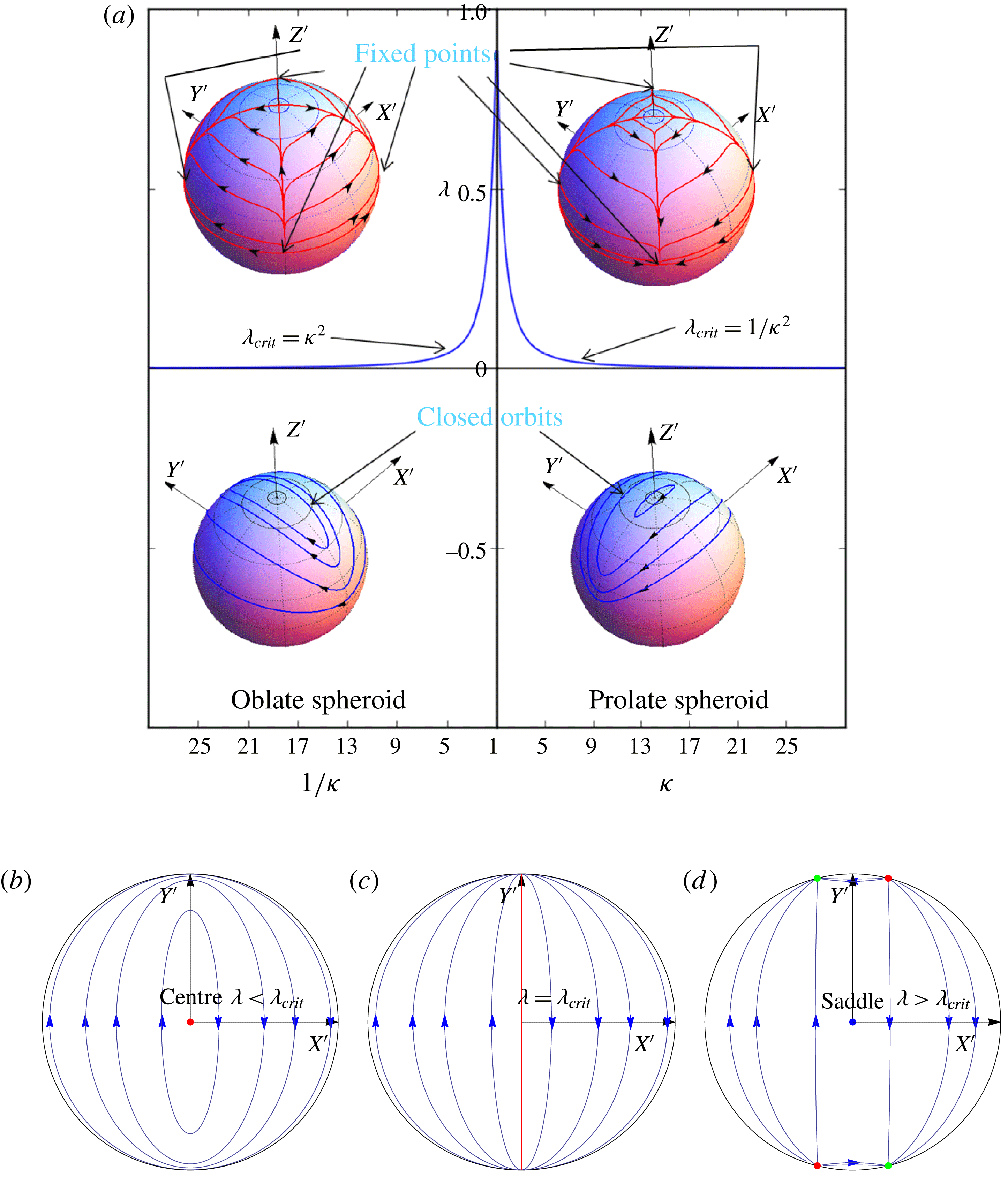
(a) The $\unicode[STIX]{x1D706}_{crit}$ curve in the $\unicode[STIX]{x1D706}{-}\unicode[STIX]{x1D705}$ plane. The blue curve corresponds to the critical $\unicode[STIX]{x1D706}$ curve which separates the open- and closed-trajectory topologies at $Re=0$ . Typical trajectory topologies, obtained from the trace of the orientation vector on a unit sphere centred at the origin starting from various initial conditions, are shown in the inset plots as blue (closed) and red (open and moving towards a stable fixed point) curves for regions above and below the $\unicode[STIX]{x1D706}_{crit}$ curve. (b–d) The transition of the intersection of the vorticity axis and the unit hemisphere from a centre below $\unicode[STIX]{x1D706}<\unicode[STIX]{x1D706}_{crit}$ to a saddle above $\unicode[STIX]{x1D706}>\unicode[STIX]{x1D706}_{crit}$ , as viewed from the vorticity axis, for an oblate spheroid. At $\unicode[STIX]{x1D706}=\unicode[STIX]{x1D706}_{crit}$ , there is a degenerate great circle of fixed points (shown in red). For $\unicode[STIX]{x1D706}>\unicode[STIX]{x1D706}_{crit}$ , there are four additional fixed points (two stable and two unstable) on the flow-gradient plane.

In figure 2(a), $\unicode[STIX]{x1D706}_{crit}$ is plotted as a function of $\unicode[STIX]{x1D705}$ . The trajectories for the spheroid orientation are closed below the $\unicode[STIX]{x1D706}_{crit}$ curve, with the minimal orbits corresponding to a pair of centres (the points of intersection of the ambient vorticity axis with the unit sphere). There are six fixed points on the unit sphere for $\unicode[STIX]{x1D706}>\unicode[STIX]{x1D706}_{crit}$ ; pairs of unstable and stable nodes in the flow-gradient plane, and the pair of centres transforming to saddle points (the indices of these fixed points add to the Euler characteristic of 2, as must be the case). Except for trajectories connecting the saddle points and unstable nodes, all remaining trajectories end in the two stable nodes. At $\unicode[STIX]{x1D706}=\unicode[STIX]{x1D706}_{crit}$ , a degenerate situation exists in which there is an entire curve of fixed points. The open- and closed-trajectory topologies on either side of the $\unicode[STIX]{x1D706}_{crit}$ curve, for both prolate and oblate spheroids, are shown in the relevant regions of figure 2(a). The aforementioned transition from a pair of centres to the six fixed points on the unit sphere is illustrated for an oblate spheroid in figure 2(b). As will be shown in later sections, in the region below the $\unicode[STIX]{x1D706}_{crit}$ curve in figure 2(a), weak inertia will result in a slow drift across the closed orbits, and the long-time orientation dynamics can be drastically different from the degenerate scenario implied by Stokesian dynamics, which predicts a continued dependence on the initial orientation. In the region above the $\unicode[STIX]{x1D706}_{crit}$ curve, weak inertia can only alter the location of the stable fixed points (corresponding to the localization of the orientation distribution for long times) by $O(Re)$ or $O(St)$ . Therefore, this region in the $\unicode[STIX]{x1D706}{-}\unicode[STIX]{x1D705}$ plane is not analysed in detail. It should be noted, however, that the corrections to the angular velocities at $O(Re)$ and $O(St)$ presented in the next two sections are valid over the entire $\unicode[STIX]{x1D706}{-}\unicode[STIX]{x1D705}$ plane.

It has been shown that in the Stokes limit, the orbits of the spheroid orientation vector in a planar linear flow ( $\unicode[STIX]{x1D706}<\unicode[STIX]{x1D706}_{crit}$ ) are the same as those of an equivalent spheroid in a simple shear flow of strength $(1-\unicode[STIX]{x1D706})$ (Prager Reference Prager1957; Bretherton Reference Bretherton1962; Hinch & Leal Reference Hinch and Leal1972). The aspect ratio of this latter spheroid is a function of $\unicode[STIX]{x1D706}$ and $\unicode[STIX]{x1D705}$ , and is given by

(4.1) $$\begin{eqnarray}\unicode[STIX]{x1D705}_{eq}=\sqrt{\frac{(\unicode[STIX]{x1D705}^{2}+1)(1-\unicode[STIX]{x1D706})+(\unicode[STIX]{x1D705}^{2}-1)(1+\unicode[STIX]{x1D706})}{(\unicode[STIX]{x1D705}^{2}+1)(1-\unicode[STIX]{x1D706})-(\unicode[STIX]{x1D705}^{2}-1)(1+\unicode[STIX]{x1D706})}}.\end{eqnarray}$$

For simple shear flow ( $\unicode[STIX]{x1D706}=0$ ), $\unicode[STIX]{x1D705}_{eq}$ is, of course, the same as $\unicode[STIX]{x1D705}$ . From (4.1), $\unicode[STIX]{x1D705}_{eq}$ varies from 1 to $\infty (0)$ for prolate (oblate) as $\unicode[STIX]{x1D706}$ increases from $-1$ to $\unicode[STIX]{x1D706}_{crit}$ . The closed trajectories in a planar linear flow are again Jeffery orbits but of the aforementioned equivalent spheroid. This would also mean that spheroids of different aspect ratios can have the same trajectories for different flows. In particular, for $\unicode[STIX]{x1D706}\rightarrow \unicode[STIX]{x1D706}_{crit}$ , a spheroid of an arbitrary aspect ratio rotates in nearly meridional trajectories similarly to a slender fibre (for prolate) or a flat disk (for oblate) in simple shear flow.

In the following sections, we interpret the weak inertial effects in terms of a drift across Stokesian trajectories in a non-orthogonal orbital coordinate system (Leal & Hinch Reference Leal and Hinch1971). The orbital coordinates ( $C,\unicode[STIX]{x1D70F}$ ) are defined such that the constant- $C$ lines coincide with the Jeffery orbits of the planar linear flow for the spheroid under consideration, while the constant- $\unicode[STIX]{x1D70F}$ lines are the same as the constant- $\unicode[STIX]{x1D719}_{j}$ contours (on the unit sphere). The orbital coordinates are related to $\unicode[STIX]{x1D703}_{j}$ and $\unicode[STIX]{x1D719}_{j}$ in terms of the equivalent aspect ratio $\unicode[STIX]{x1D705}_{eq}$ ,

(4.2) $$\begin{eqnarray}\displaystyle & \displaystyle C=\tan \unicode[STIX]{x1D703}_{j}\frac{\sqrt{(\unicode[STIX]{x1D705}_{eq}^{2}\sin ^{2}\unicode[STIX]{x1D719}_{j}+\cos ^{2}\unicode[STIX]{x1D719}_{j})}}{\unicode[STIX]{x1D705}_{eq}}, & \displaystyle\end{eqnarray}$$

(4.3) $$\begin{eqnarray}\displaystyle & \displaystyle \unicode[STIX]{x1D70F}=\tan ^{-1}\left(\frac{1}{\unicode[STIX]{x1D705}_{eq}\tan \unicode[STIX]{x1D719}_{j}}\right)\!. & \displaystyle\end{eqnarray}$$

Here, $C$ varies from 0 to $\infty$ , with $C=0$ and $C=\infty$ being the spinning and tumbling orbits respectively, with the finite- $C$ orbits corresponding to three-dimensional precessional motions. The angular velocity vector of the spheroid in the tumbling and spinning orbits is respectively perpendicular and parallel to $\boldsymbol{p}$ . For any fixed $C$ , the orbit phase $\unicode[STIX]{x1D70F}$ varies from $0$ to $2\unicode[STIX]{x03C0}$ and changes at a constant rate (despite $\unicode[STIX]{x1D719}_{j}$ changing at a variable rate). The equations for the rates of change take a simple form in the orbital coordinate system, and are given by

(4.4) $$\begin{eqnarray}\displaystyle & \displaystyle \frac{\text{d}C}{\text{d}t}=0, & \displaystyle\end{eqnarray}$$

(4.5) $$\begin{eqnarray}\displaystyle & \displaystyle \frac{\text{d}\unicode[STIX]{x1D70F}}{\text{d}t}=\frac{(1-\unicode[STIX]{x1D706})\unicode[STIX]{x1D705}_{eq}}{(\unicode[STIX]{x1D705}_{eq}^{2}+1)}. & \displaystyle\end{eqnarray}$$

Evidently, $C$ does not change in the Stokes limit. It should be noted that the above equations are valid for $-1<\unicode[STIX]{x1D706}<\unicode[STIX]{x1D706}_{crit}$ . In the limit of $\unicode[STIX]{x1D706}\rightarrow -1$ , that is, the trivial case of solid-body rotation, $\unicode[STIX]{x1D705}_{eq}$ is 1, and the orbits are merely circles transverse to the ambient vorticity. In the limit of $\unicode[STIX]{x1D706}\rightarrow \unicode[STIX]{x1D706}_{crit}^{-}$ , $\unicode[STIX]{x1D705}_{eq}\rightarrow \infty$ ( $0$ ) for a prolate (an oblate) spheroid, and the angular velocity $\text{d}\unicode[STIX]{x1D70F}/\text{d}t\rightarrow 0$ , consistent with the transition to an open-trajectory topology across $\unicode[STIX]{x1D706}=\unicode[STIX]{x1D706}_{crit}$ .

5 The effect of particle inertia: massive spheroids ( $Re=0$ and $St\ll 1$ )

In this section, we investigate the effect of particle inertia on the orientation dynamics of a spheroid in a planar linear flow. This analysis is important for finding the orientation of particles in solid–gas systems where $\unicode[STIX]{x1D70C}_{p}\gg \unicode[STIX]{x1D70C}_{f}$ ; an example in this regard is the orientation distribution of ice crystals in atmospheric turbulence, which is relevant to the determination of cirrus cloud reflectivities, a crucial component of the Earth–atmosphere radiation budget (Liou Reference Liou1986). The $O(St)$ correction to the angular velocity of a spheroid in a planar linear flow was derived in an invariant form by Einarsson et al. (Reference Einarsson, Angilella and Mehlig2014). However, they restricted their analysis to finding the orbit that is stabilized at long times for the particular case of simple shear flow ( $\unicode[STIX]{x1D706}=0$ ). Below, we present the orbits stabilized by particle inertia in the entire $\unicode[STIX]{x1D706}{-}\unicode[STIX]{x1D705}$ plane ( $\unicode[STIX]{x1D706}<\unicode[STIX]{x1D706}_{crit}$ ; see figure 2). For completeness, we present the calculation of the $O(St)$ correction to the angular velocity using (2.4) by setting $Re=0$ , whence (2.4) reduces to

(5.1) $$\begin{eqnarray}\displaystyle \unicode[STIX]{x1D734}_{1}\boldsymbol{\cdot }\unicode[STIX]{x1D647}_{2} & = & \displaystyle \unicode[STIX]{x1D71E}:\int _{S_{p}}\boldsymbol{x}(\unicode[STIX]{x1D72E}^{(2)}\boldsymbol{\cdot }\boldsymbol{n})\,\text{d}S+St\,\frac{\text{d}}{\text{d}t}({\unicode[STIX]{x1D644}_{p}\boldsymbol{\cdot }\unicode[STIX]{x1D734}}_{1}).\end{eqnarray}$$

The second term on the right-hand side gives the correction due to the particle angular acceleration. As mentioned earlier, it is convenient to evaluate the correction in the body-aligned coordinate system ( $XYZ$ in figure 1 f), which rotates with $\unicode[STIX]{x1D734}_{jeff}^{t}$ . Noting that the rate of change in the space-fixed coordinate system is related to the rate of change in the body-aligned one as $\text{d}/\text{d}t(.)=(\text{d}/\text{d}t(.))_{b}+\unicode[STIX]{x1D734}_{jeff}^{t}\wedge (.)$ , the subscript ‘ $b$ ’ denoting the $XYZ$ system, and that the moment of inertia tensor is now a constant, (5.1) takes the form

(5.2) $$\begin{eqnarray}\displaystyle \unicode[STIX]{x1D734}_{1}\boldsymbol{\cdot }\unicode[STIX]{x1D647}^{(2)} & = & \displaystyle \unicode[STIX]{x1D71E}:\int _{S_{p}}\boldsymbol{x}(\unicode[STIX]{x1D72E}^{(2)}\boldsymbol{\cdot }\boldsymbol{n})\,\text{d}S+St\,\left[\unicode[STIX]{x1D644}_{p}\boldsymbol{\cdot }\left(\frac{\text{d}\unicode[STIX]{x1D734}_{1}}{\text{d}t}\right)_{b}+\unicode[STIX]{x1D734}_{jeff}^{t}\wedge (\unicode[STIX]{x1D644}_{p}\boldsymbol{\cdot }\unicode[STIX]{x1D734}_{1})\right].\end{eqnarray}$$

Using a regular expansion of the form $\unicode[STIX]{x1D734}_{1}=\unicode[STIX]{x1D734}_{jeff}+St\,\unicode[STIX]{x1D734}_{1St}^{(1)}+O(St^{2})$ for the particle angular velocity, one obtains

(5.3) $$\begin{eqnarray}\displaystyle \unicode[STIX]{x1D734}_{1St}^{(1)}\boldsymbol{\cdot }\unicode[STIX]{x1D647}^{(2)} & = & \displaystyle \unicode[STIX]{x1D644}_{p}\boldsymbol{\cdot }\frac{\text{d}\unicode[STIX]{x1D734}_{jeff}}{\text{d}t_{jeff}}+\unicode[STIX]{x1D734}_{jeff}^{t}\wedge (\unicode[STIX]{x1D644}_{p}\boldsymbol{\cdot }\unicode[STIX]{x1D734}_{jeff}),\end{eqnarray}$$

at $O(St)$ . In (5.3), to leading order, $(\text{d}/\text{d}t)_{b}$ is replaced by $(\text{d}/\text{d}t)_{jeff}$ , where the latter denotes the rate of change along the closed orbit in the Stokes limit, given by (2.2) and (2.3) in terms of $\unicode[STIX]{x1D703}_{j}$ and $\unicode[STIX]{x1D719}_{j}$ . The rates of change of $\unicode[STIX]{x1D719}_{j}$ and $\unicode[STIX]{x1D703}_{j}$ , at $O(St)$ , can be obtained from (5.3), $\dot{\unicode[STIX]{x1D719}}_{jSt}=-\unicode[STIX]{x1D6FA}_{1St}^{(1)x}/\sin \unicode[STIX]{x1D703}_{j}$ and $\dot{\unicode[STIX]{x1D703}}_{jSt}=\unicode[STIX]{x1D6FA}_{1St}^{(1)y}$ , and are given by

(5.4) $$\begin{eqnarray}\displaystyle \left(\frac{\text{d}\unicode[STIX]{x1D703}_{j}}{\text{d}t}\right)_{St} & = & \displaystyle \sin \unicode[STIX]{x1D703}_{j}\cos \unicode[STIX]{x1D703}_{j}\left[F_{1}^{p}(\unicode[STIX]{x1D709}_{0},\unicode[STIX]{x1D706})+F_{2}^{p}(\unicode[STIX]{x1D709}_{0},\unicode[STIX]{x1D706})\cos 2\unicode[STIX]{x1D719}_{j}+F_{3}^{p}(\unicode[STIX]{x1D709}_{0},\unicode[STIX]{x1D706})\cos 2\unicode[STIX]{x1D703}_{j}\right.\nonumber\\ \displaystyle & & \displaystyle +\,F_{4}^{p}(\unicode[STIX]{x1D709}_{0},\unicode[STIX]{x1D706})\cos 4\unicode[STIX]{x1D719}_{j}+\left.F_{5}^{p}(\unicode[STIX]{x1D709}_{0},\unicode[STIX]{x1D706})\cos (2\unicode[STIX]{x1D703}_{j}-4\unicode[STIX]{x1D719}_{j})+F_{6}^{p}(\unicode[STIX]{x1D709}_{0},\unicode[STIX]{x1D706})\cos (2\unicode[STIX]{x1D703}_{j}+4\unicode[STIX]{x1D719}_{j})\right],\nonumber\\ \displaystyle & & \displaystyle\end{eqnarray}$$

(5.5) $$\begin{eqnarray}\displaystyle \left(\frac{\text{d}\unicode[STIX]{x1D719}_{j}}{\text{d}t}\right)_{St} & = & \displaystyle \sin \unicode[STIX]{x1D719}_{j}\cos \unicode[STIX]{x1D719}_{j}\left[G_{1}^{p}(\unicode[STIX]{x1D709}_{0},\unicode[STIX]{x1D706})+G_{2}^{p}(\unicode[STIX]{x1D709}_{0},\unicode[STIX]{x1D706})\cos 2\unicode[STIX]{x1D703}_{j}+G_{3}^{p}(\unicode[STIX]{x1D709}_{0},\unicode[STIX]{x1D706})\cos 2\unicode[STIX]{x1D719}_{j}\right.\nonumber\\ \displaystyle & & \displaystyle \left.+\,G_{4}^{p}(\unicode[STIX]{x1D709}_{0},\unicode[STIX]{x1D706})\cos 2\unicode[STIX]{x1D703}_{j}\cos 2\unicode[STIX]{x1D719}_{j}\right].\end{eqnarray}$$

The functions of $\unicode[STIX]{x1D709}_{0}$ and $\unicode[STIX]{x1D706}$ that appear above for a prolate spheroid are given in appendix B. The expressions in (5.4) and (5.5) are consistent with those given by Einarsson et al. (Reference Einarsson, Angilella and Mehlig2014).

In the analysis that follows, we investigate the effect of the inertial corrections given in (5.4) and (5.5) on the trajectory of the orientation vector for all ( $\unicode[STIX]{x1D706}$ , $\unicode[STIX]{x1D705}$ ) combinations below the $\unicode[STIX]{x1D706}_{crit}$ curve in figure 2. There are two approaches to carry out this investigation. The first, brute-force, approach is to numerically integrate the differential equations governing $\unicode[STIX]{x1D703}_{j}$ and $\unicode[STIX]{x1D719}_{j}$ , obtained by adding the angular velocities given in (5.4) and (5.5) and the corresponding leading-order angular velocities given in (2.3) and (2.2), to obtain the inertial trajectory on the unit sphere. 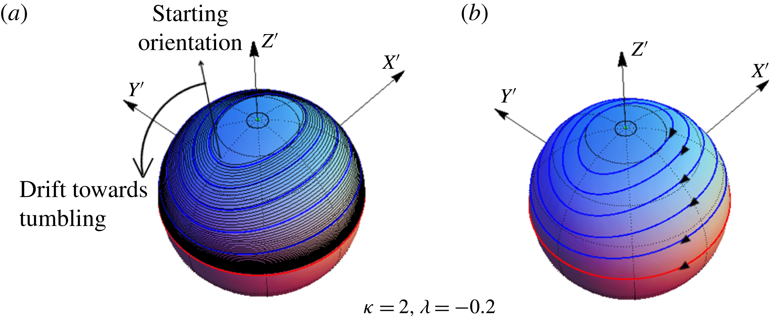The trajectory obtained in the manner described above, starting from a particular initial condition ( $St=1$ , $\unicode[STIX]{x1D703}_{j0}=0.5$ , $\unicode[STIX]{x1D719}_{j0}=\unicode[STIX]{x03C0}$ ), is shown in figure 3(a) for a prolate spheroid of aspect ratio 2 in an elliptic flow with $\unicode[STIX]{x1D706}=-0.2$ . The Jeffery orbits, for the same set of parameters, are plotted in figure 3(b) for purposes of comparison. As is evident, the spheroid drifts towards the tumbling orbit (red curve on the unit sphere in figure 3 a). It is cumbersome to repeat this exercise for the whole ( $\unicode[STIX]{x1D705}$ – $\unicode[STIX]{x1D706}$ ) plane below the $\unicode[STIX]{x1D706}_{crit}$ curve in figure 2, and for all possible initial orientations, and this is not pursued further.

Figure 3.

(a) The finite- $St$ inertial trajectory (black) is plotted on a unit sphere for a prolate spheroid with $\unicode[STIX]{x1D705}=2$ in an elliptic linear flow with $\unicode[STIX]{x1D706}=-0.2$ . For purposes of illustration, the Stokes number is chosen to be unity. The tumbling orbit is the red curve. The blue curves on the unit sphere in (a) and (b) are the Jeffery orbits.

In the second approach, the orbital drift, defined as the change in orbit constant per Jeffery period, is evaluated. To do this, one first differentiates (4.2), to obtain

(5.6) $$\begin{eqnarray}\displaystyle \frac{\text{d}C}{\text{d}t} & = & \displaystyle \frac{C}{\sin \unicode[STIX]{x1D703}_{j}\cos \unicode[STIX]{x1D703}_{j}}\frac{\text{d}\unicode[STIX]{x1D703}_{j}}{\text{d}t}+\frac{C(\unicode[STIX]{x1D705}_{eq}^{2}-1)\cos \unicode[STIX]{x1D719}_{j}\sin \unicode[STIX]{x1D719}_{j}}{\unicode[STIX]{x1D705}_{eq}^{2}\sin ^{2}\unicode[STIX]{x1D719}_{j}+\cos ^{2}\unicode[STIX]{x1D719}_{j}}\frac{\text{d}\unicode[STIX]{x1D719}_{j}}{\text{d}t}.\end{eqnarray}$$

Since $\text{d}C/\text{d}t=0$ at leading order, equation (5.6) takes the form

(5.7) $$\begin{eqnarray}\displaystyle \frac{\text{d}C}{\text{d}t} & = & \displaystyle St\,C\left[\frac{1}{\sin \unicode[STIX]{x1D703}_{j}\cos \unicode[STIX]{x1D703}_{j}}\left(\frac{\text{d}\unicode[STIX]{x1D703}_{j}}{\text{d}t}\right)_{St}+\frac{(\unicode[STIX]{x1D705}_{eq}^{2}-1)\cos \unicode[STIX]{x1D719}_{j}\sin \unicode[STIX]{x1D719}_{j}}{\unicode[STIX]{x1D705}_{eq}^{2}\sin ^{2}\unicode[STIX]{x1D719}_{j}+\cos ^{2}\unicode[STIX]{x1D719}_{j}}\left(\frac{\text{d}\unicode[STIX]{x1D719}_{j}}{\text{d}t}\right)_{St}\right],\end{eqnarray}$$

where $(\text{d}\unicode[STIX]{x1D703}_{j}/\text{d}t)_{St}$ and $(\text{d}\unicode[STIX]{x1D719}_{j}/\text{d}t)_{St}$ are given by (5.4) and (5.5). As expected, the change in $C$ is at $O(St)$ , and leads to an inertial trajectory where the spheroid orientation vector spirals towards either the flow-gradient plane or the spinning orbit. For $St\ll 1$ , this spiralling is tight, with each turn of the spiral closely approximating a Jeffery orbit (see figure 3 a). The orbital drift can then be conveniently characterized by the pitch of the inertial spiral measured in units of $C$ . This pitch, $\unicode[STIX]{x0394}C$ , defined at leading order as the change in $C$ during a single Jeffery period ( $T_{jeff}=2\unicode[STIX]{x03C0}(\unicode[STIX]{x1D705}_{eq}^{2}+1)/((1-\unicode[STIX]{x1D706})\unicode[STIX]{x1D705}_{eq})$ ), is given by

(5.8) $$\begin{eqnarray}\displaystyle \unicode[STIX]{x0394}C_{p} & = & \displaystyle \displaystyle \int _{0}^{T_{jeff}}\frac{\text{d}C}{\text{d}t}\,\text{d}t,\end{eqnarray}$$

(5.9) $$\begin{eqnarray}\displaystyle \phantom{\unicode[STIX]{x0394}C_{p}} & = & \displaystyle St\frac{\unicode[STIX]{x1D705}_{eq}^{2}+1}{(1-\unicode[STIX]{x1D706})\unicode[STIX]{x1D705}_{eq}}\int _{0}^{2\unicode[STIX]{x03C0}}C\left(\frac{1}{\sin \unicode[STIX]{x1D703}_{j}\cos \unicode[STIX]{x1D703}_{j}}\left(\frac{\text{d}\unicode[STIX]{x1D703}_{j}}{\text{d}t}\right)_{St}\right.\nonumber\\ \displaystyle & & \displaystyle \left.+\,\frac{(\unicode[STIX]{x1D705}_{eq}^{2}-1)\cos \unicode[STIX]{x1D719}_{j}\sin \unicode[STIX]{x1D719}_{j}}{\unicode[STIX]{x1D705}_{eq}^{2}\sin ^{2}\unicode[STIX]{x1D719}_{j}+\cos ^{2}\unicode[STIX]{x1D719}_{j}}\left(\frac{\text{d}\unicode[STIX]{x1D719}_{j}}{\text{d}t}\right)_{St}\right)\,\text{d}\unicode[STIX]{x1D70F},\end{eqnarray}$$

where the subscript ‘ $p$ ’ denotes particle inertia. The $\unicode[STIX]{x1D70F}$ integrals in (5.9) are to be evaluated for fixed $C$ , implying closeness of the inertial spiralling trajectory at a given point to a Jeffery orbit passing through the same point. Using (5.4) and (5.5), one obtains

(5.10) $$\begin{eqnarray}\displaystyle \unicode[STIX]{x0394}C_{p} & = & \displaystyle St\,C\,\frac{\unicode[STIX]{x1D705}_{eq}^{2}+1}{(1-\unicode[STIX]{x1D706})\unicode[STIX]{x1D705}_{eq}}\left\{\!\left[I_{1}F_{1}^{p}(\unicode[STIX]{x1D709}_{0},\unicode[STIX]{x1D706})+I_{2}F_{2}^{p}(\unicode[STIX]{x1D709}_{0},\unicode[STIX]{x1D706})+I_{3}F_{3}^{p}(\unicode[STIX]{x1D709}_{0},\unicode[STIX]{x1D706})+I_{4}F_{4}^{p}(\unicode[STIX]{x1D709}_{0},\unicode[STIX]{x1D706})\right.\right.\nonumber\\ \displaystyle & & \displaystyle \left.+\,I_{5}F_{5}^{p}(\unicode[STIX]{x1D709}_{0},\unicode[STIX]{x1D706})+I_{6}F_{6}^{p}(\unicode[STIX]{x1D709}_{0},\unicode[STIX]{x1D706})\right]\nonumber\\ \displaystyle & & \displaystyle \left.+\left[J_{1}G_{1}^{p}(\unicode[STIX]{x1D709}_{0},\unicode[STIX]{x1D706})+J_{2}G_{2}^{p}(\unicode[STIX]{x1D709}_{0},\unicode[STIX]{x1D706})+J_{3}G_{3}^{p}(\unicode[STIX]{x1D709}_{0},\unicode[STIX]{x1D706})+J_{4}G_{4}^{p}(\unicode[STIX]{x1D709}_{0},\unicode[STIX]{x1D706})\right]\!\right\}.\end{eqnarray}$$

The expressions for $I_{1}$ – $J_{4}$ , as functions of $C$ and $\unicode[STIX]{x1D705}_{eq}$ , are given in appendix C. The orbital drift approximation in (5.10) has reduced the need from a consideration of all possible initial orientations in the brute-force approach mentioned earlier to a one-dimensional examination of all possible values of $C$ . The average change, however, should be much less than $C$ , and, therefore, the above analysis implies $((\unicode[STIX]{x0394}C)/C)\ll 1$ . It can be seen from (5.10) that this condition breaks down when $St\sim \unicode[STIX]{x1D705}_{eq}(1/\unicode[STIX]{x1D705}_{eq})$ , corresponding to oblate (prolate) spheroids with $\unicode[STIX]{x1D705}_{eq}\ll 1$ ( $\unicode[STIX]{x1D705}_{eq}\gg 1$ ) (the $F_{i}$ and $G_{i}$ values remain of order unity except in the limit $\unicode[STIX]{x1D705}_{eq}\rightarrow \infty$ , that is, for slender fibres in a flow close to simple shear; in this case, the $F_{i}$ and $G_{i}$ values are $O(1/\log \unicode[STIX]{x1D705}_{eq})$ , and the $St$ corresponding to the breakdown is $O(\log \unicode[STIX]{x1D705}_{eq}/\unicode[STIX]{x1D705}_{eq})$ ). This would mean that close to the $\unicode[STIX]{x1D706}_{crit}$ curve in figure 2, the orbital drift approximation becomes increasingly restrictive, being valid only when $St\ll \unicode[STIX]{x1D705}_{eq}$ or $1/\unicode[STIX]{x1D705}_{eq}$ . It is shown later, in § 8, that the orbital drift interpretation, motivated here using physical arguments, emerges naturally as the leading-order term in the framework of a multiple time scale analysis. The limitations of this interpretation in the limits of $\unicode[STIX]{x1D705}_{eq}\rightarrow 0$ and $\infty$ are also discussed therein.

The orbital drift in (5.10) is a function of $C$ and $\unicode[STIX]{x1D706}$ as well as $\unicode[STIX]{x1D705}$ (through $\unicode[STIX]{x1D709}_{0}$ which is the inverse of the spheroid eccentricity). The drift is positive for a prolate spheroid of any aspect ratio in a planar linear flow with a non-positive $\unicode[STIX]{x1D706}$ (all elliptic linear flows, including the limiting case of solid-body rotation and simple shear flow). Thus, a prolate spheroid in any flow with $\unicode[STIX]{x1D706}\leqslant 0$ approaches the tumbling orbit for long times; this is expected for $\unicode[STIX]{x1D706}=-1$ , where one expects the particle to centrifuge outward towards the tumbling orbit (in the absence of the $O(Re)$ contribution arising from centrifugal buoyancy). 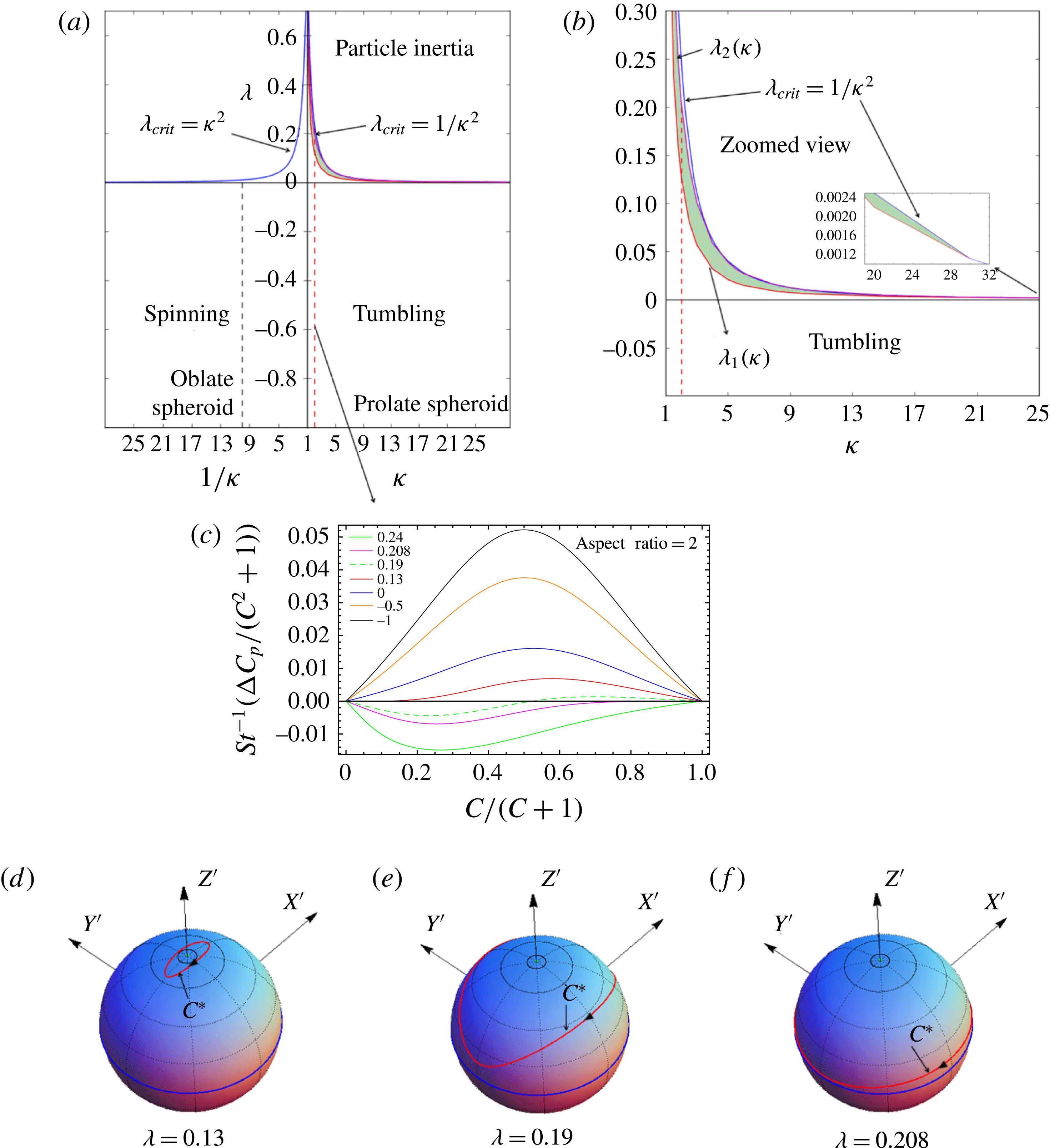This is noted in the fourth quadrant of the $\unicode[STIX]{x1D706}{-}\unicode[STIX]{x1D705}$ plane in figure 4(a). In a hyperbolic flow ( $0<\unicode[STIX]{x1D706}<\unicode[STIX]{x1D706}_{crit}$ ), the tumbling orbit continues to be the long-time orientation limit for a prolate spheroid with $\unicode[STIX]{x1D705}$ greater than approximately 30. However, if the aspect ratio of the spheroid is smaller than 30, the tumbling orbit is stabilized at long times only until a particular $\unicode[STIX]{x1D706}_{1}(\unicode[STIX]{x1D705})$ ( $0<\unicode[STIX]{x1D706}_{1}<\unicode[STIX]{x1D706}_{crit}$ ), indicated by the red curve in the first quadrant of figure 4(a). For these aspect ratios, if $\unicode[STIX]{x1D706}$ is larger than $\unicode[STIX]{x1D706}_{1}$ , a repeller (a Jeffery orbit at the order of approximation considered) exists on each unit hemisphere, dividing it into two distinct basins of attraction, with the attractor being the tumbling orbit for one basin and the spinning orbit for the other. The shaded region in figure 4(a) corresponds to all those $\unicode[STIX]{x1D706}$ values for which two distinct basins of attraction exist on the unit hemisphere. Eventually, with increasing $\unicode[STIX]{x1D706}$ , the spinning orbit becomes the sole attractor at a particular $\unicode[STIX]{x1D706}_{2}(\unicode[STIX]{x1D705})~(\unicode[STIX]{x1D706}_{1}<\unicode[STIX]{x1D706}_{2})$ , indicated by the magenta curve in the zoomed plot in figure 4(b), and remains so for the narrow range of $\unicode[STIX]{x1D706}$ in the interval $\unicode[STIX]{x1D706}_{2}(\unicode[STIX]{x1D705})<\unicode[STIX]{x1D706}<\unicode[STIX]{x1D706}_{crit}$ , with $\unicode[STIX]{x1D706}_{2}\rightarrow \unicode[STIX]{x1D706}_{crit}$ for an aspect ratio approximately equal to 30.

Figure 4.

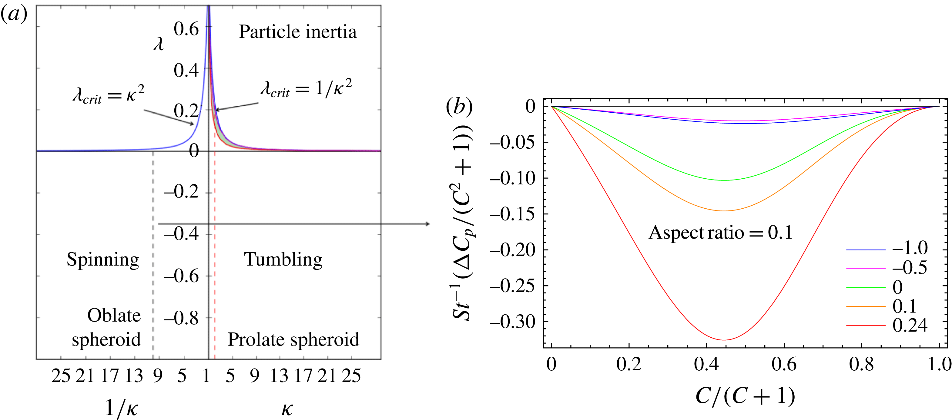
(a) The orbit(s) stabilized at long times, due to particle inertia, are identified for all combinations of $\unicode[STIX]{x1D706}$ – $\unicode[STIX]{x1D705}$ below the $\unicode[STIX]{x1D706}_{crit}$ curve (blue curve). The red curve (the zoomed view of this curve is denoted by $\unicode[STIX]{x1D706}_{1}(\unicode[STIX]{x1D705})$ in b) denotes the locus of $(\unicode[STIX]{x1D706},\unicode[STIX]{x1D705})$ values at which the repeller emerges from the spinning orbit. The shaded region denotes the $(\unicode[STIX]{x1D706},\unicode[STIX]{x1D705})$ combinations for which there is a repeller on the unit hemisphere. (b) A zoomed view that shows the bounding curves $\unicode[STIX]{x1D706}_{1}(\unicode[STIX]{x1D705})$ and $\unicode[STIX]{x1D706}_{2}(\unicode[STIX]{x1D705})$ . (c) The orbital drift is plotted against $C/(C+1)$ for a prolate spheroid of $\unicode[STIX]{x1D705}=2$ for various values of $\unicode[STIX]{x1D706}$ . The $C$ at which drift changes sign corresponds to the repeller ( $C^{\ast }$ ) location, which migrates from the spinning orbit ( $C/(C+1)=0$ ) to the tumbling orbit ( $C/(C+1)=0$ ) with increasing $\unicode[STIX]{x1D706}$ . The repeller orbits (red) are plotted for a prolate spheroid of aspect ratio 2, and for $\unicode[STIX]{x1D706}$ values of (d) 0.13 (e) 0.19 and (f) 0.208 (the tumbling orbit in all cases is shown in blue).

Figure 5.

(a) The orbits stabilized at long times, due to particle inertia, are indicated. (b) The orbital drift is plotted against $C/(C+1)$ for an oblate spheroid of aspect ratio 0.1 for various values of $\unicode[STIX]{x1D706}$ . The drift does not change sign for an oblate spheroid.

In figure 4(c), the orbital drift $\unicode[STIX]{x0394}C_{p}$ is plotted against $C/(C+1)$ for a particular prolate spheroid with $\unicode[STIX]{x1D705}=2$ for different values of $\unicode[STIX]{x1D706}$ . The drift is positive for all $\unicode[STIX]{x1D706}$ values below $\unicode[STIX]{x1D706}\approx 0.13$ ( $\unicode[STIX]{x1D706}_{1}$ for $\unicode[STIX]{x1D705}=2$ ), and the long-time orientation dynamics approaches the tumbling orbit. As $\unicode[STIX]{x1D706}$ becomes larger than $0.13$ , the sign of the drift changes across a critical $C$ (Jeffery orbit with $C=C^{\ast }$ , say). This Jeffery orbit, which acts as a repeller, emerges from the spinning orbit at around $\unicode[STIX]{x1D706}=0.13$ ( $\unicode[STIX]{x1D706}_{1}$ ), and with increasing $\unicode[STIX]{x1D706}$ , moves towards the tumbling orbit, eventually coinciding with it at $\unicode[STIX]{x1D706}\approx 0.20$ ( $\unicode[STIX]{x1D706}_{2}$ for $\unicode[STIX]{x1D705}=2$ ). The repeller orbits for $\unicode[STIX]{x1D705}=2$ at various $\unicode[STIX]{x1D706}$ values are plotted on the unit sphere in figure 4(d–f).

The long-time orientation dynamics of an oblate spheroid is simpler compared with that of the prolate spheroid above. An oblate spheroid drifts towards the spinning orbit irrespective of its initial orientation and aspect ratio in any planar linear flow with $\unicode[STIX]{x1D706}<\unicode[STIX]{x1D706}_{crit}$ . In figure 5(b), the orbital drift is plotted against $C/(C+1)$ for various $\unicode[STIX]{x1D706}$ values for an oblate spheroid of aspect ratio 0.1, and is negative irrespective of $C$ and $\unicode[STIX]{x1D706}$ .

6 The effect of fluid inertia ( $St=0$ and $Re\ll 1$ )

In this section, we investigate the effect of fluid inertia on the orientation dynamics of a spheroid in a planar linear flow. The effect of fluid inertia on the orientation dynamics in the particular case of simple shear flow ( $\unicode[STIX]{x1D706}=0$ ) has already been analysed in earlier works (Einarsson et al. Reference Einarsson, Candelier, Lundell, Angilella and Mehlig2015; Dabade et al. Reference Dabade, Marath and Subramanian2016). It was shown that, depending on the aspect ratio as well as the ratio $St/Re$ , the effect of fluid inertia can either oppose or complement that due to particle inertia. In planar linear flow, the rates of change of $\unicode[STIX]{x1D719}_{j}$ and $\unicode[STIX]{x1D703}_{j}$ , at $O(Re)$ , are obtained by evaluating the integrals proportional to $Re$ on the right-hand side of (2.4), using the velocity fields given in § 3, and are given by

(6.1) $$\begin{eqnarray}\displaystyle \displaystyle \left(\frac{\text{d}\unicode[STIX]{x1D703}_{j}}{\text{d}t}\right)_{Re} & = & \displaystyle \sin \unicode[STIX]{x1D703}_{j}\cos \unicode[STIX]{x1D703}_{j}\left[F_{1}^{f}(\unicode[STIX]{x1D709}_{0},\unicode[STIX]{x1D706})+F_{2}^{f}(\unicode[STIX]{x1D709}_{0},\unicode[STIX]{x1D706})\cos 2\unicode[STIX]{x1D719}_{j}+F_{3}^{f}(\unicode[STIX]{x1D709}_{0},\unicode[STIX]{x1D706})\cos 2\unicode[STIX]{x1D703}_{j}\right.\nonumber\\ \displaystyle & & \displaystyle \displaystyle +\,F_{4}^{f}(\unicode[STIX]{x1D709}_{0},\unicode[STIX]{x1D706})\cos 4\unicode[STIX]{x1D719}_{j}\left.+\,F_{5}^{f}(\unicode[STIX]{x1D709}_{0},\unicode[STIX]{x1D706})\cos (2\unicode[STIX]{x1D703}_{j}-4\unicode[STIX]{x1D719}_{j})+F_{6}^{f}(\unicode[STIX]{x1D709}_{0},\unicode[STIX]{x1D706})\cos (2\unicode[STIX]{x1D703}_{j}+4\unicode[STIX]{x1D719}_{j})\right],\nonumber\\ \displaystyle & & \displaystyle\end{eqnarray}$$

(6.2) $$\begin{eqnarray}\displaystyle \displaystyle \left(\frac{\text{d}\unicode[STIX]{x1D719}_{j}}{\text{d}t}\right)_{Re} & = & \displaystyle \sin \unicode[STIX]{x1D719}_{j}\cos \unicode[STIX]{x1D719}_{j}\left[G_{1}^{f}(\unicode[STIX]{x1D709}_{0},\unicode[STIX]{x1D706})+G_{2}^{f}(\unicode[STIX]{x1D709}_{0},\unicode[STIX]{x1D706})\cos 2\unicode[STIX]{x1D703}_{j}+G_{3}^{f}(\unicode[STIX]{x1D709}_{0},\unicode[STIX]{x1D706})\cos 2\unicode[STIX]{x1D719}_{j}\right.\nonumber\\ \displaystyle & & \displaystyle \left.+\,G_{4}^{f}(\unicode[STIX]{x1D709}_{0},\unicode[STIX]{x1D706})\cos (2\unicode[STIX]{x1D703}_{j})\cos (2\unicode[STIX]{x1D719}_{j})\right].\end{eqnarray}$$

The functions of $\unicode[STIX]{x1D709}_{0}$ and $\unicode[STIX]{x1D706}$ that appear above for a prolate spheroid are given in appendix B. The analytical approach introduced in § 5 is used to evaluate the orbital drift due to fluid inertia, which is given by

(6.3) $$\begin{eqnarray}\displaystyle \unicode[STIX]{x0394}C_{f} & = & \displaystyle Re\,C\,\frac{\unicode[STIX]{x1D705}_{eq}^{2}+1}{(1-\unicode[STIX]{x1D706})\unicode[STIX]{x1D705}_{eq}}\left\{\!\left[I_{1}F_{1}^{f}(\unicode[STIX]{x1D709}_{0},\unicode[STIX]{x1D706})+I_{2}F_{2}^{f}(\unicode[STIX]{x1D709}_{0},\unicode[STIX]{x1D706})+I_{3}F_{3}^{f}(\unicode[STIX]{x1D709}_{0},\unicode[STIX]{x1D706})+I_{4}F_{4}^{f}(\unicode[STIX]{x1D709}_{0},\unicode[STIX]{x1D706})\right.\right.\nonumber\\ \displaystyle & & \displaystyle \left.+\,I_{5}F_{5}^{f}(\unicode[STIX]{x1D709}_{0},\unicode[STIX]{x1D706})+I_{6}F_{6}^{f}(\unicode[STIX]{x1D709}_{0},\unicode[STIX]{x1D706})\right]\nonumber\\ \displaystyle & & \displaystyle \left.+\left[J_{1}G_{1}^{f}(\unicode[STIX]{x1D709}_{0},\unicode[STIX]{x1D706})+J_{2}G_{2}^{f}(\unicode[STIX]{x1D709}_{0},\unicode[STIX]{x1D706})+J_{3}G_{3}^{f}(\unicode[STIX]{x1D709}_{0},\unicode[STIX]{x1D706})+J_{4}G_{4}^{f}(\unicode[STIX]{x1D709}_{0},\unicode[STIX]{x1D706})\right]\!\right\},\end{eqnarray}$$

where the $I_{i}$ and $J_{i}$ terms are the same as those in § 5.

Figure 6.

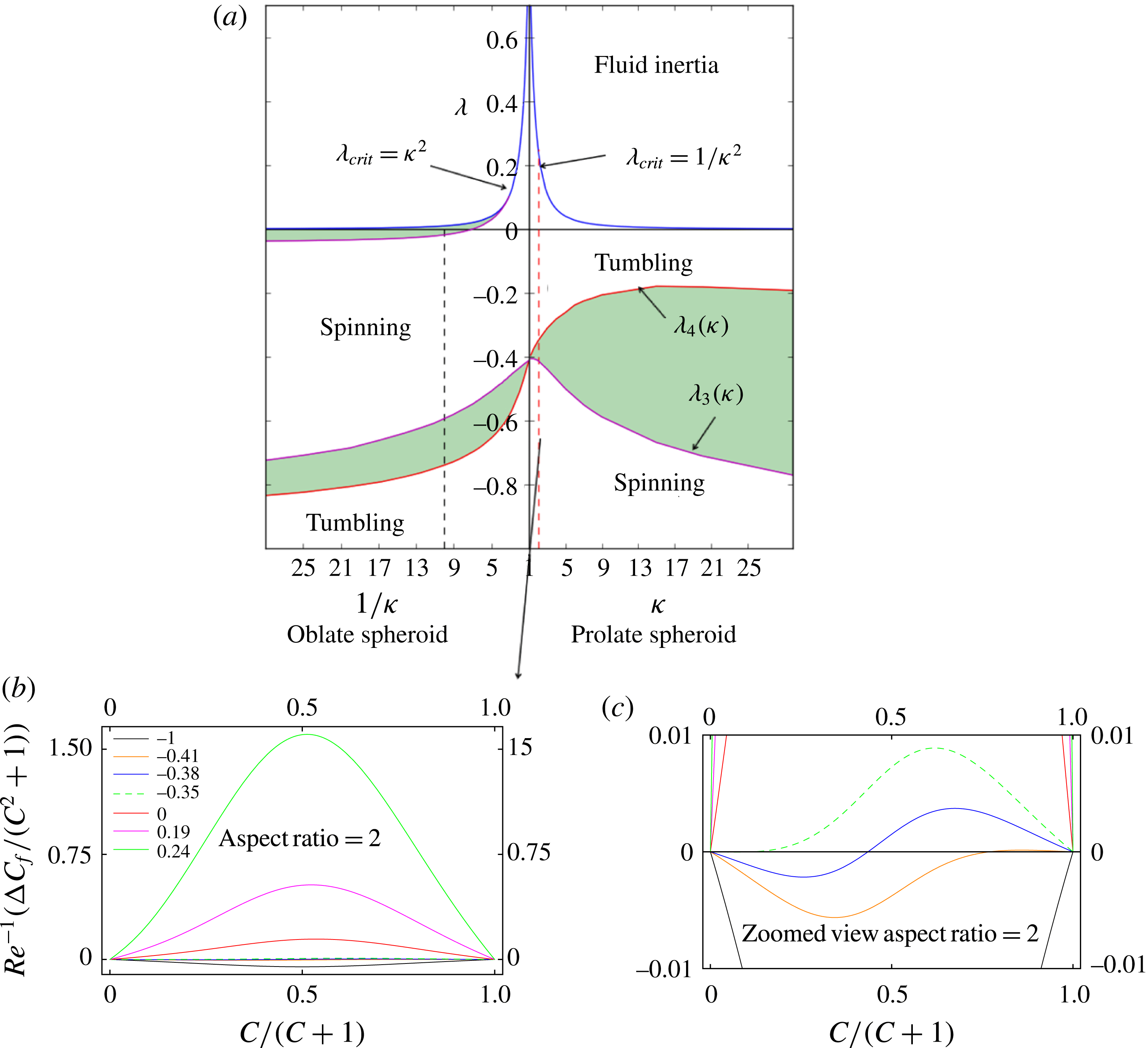
(a) The orbit(s) that are stabilized at long times, due to fluid inertia, are identified for all ( $\unicode[STIX]{x1D706}$ , $\unicode[STIX]{x1D705}$ ) combinations below the $\unicode[STIX]{x1D706}_{crit}$ curve (blue). The shaded regions correspond to the $(\unicode[STIX]{x1D706},\unicode[STIX]{x1D705})$ combinations for which there are two distinct basins of attraction separated by a repeller. The red ( $\unicode[STIX]{x1D706}_{4}(\unicode[STIX]{x1D705})$ ) and magenta ( $\unicode[STIX]{x1D706}_{3}(\unicode[STIX]{x1D705})$ ) curves correspond to all combinations of $(\unicode[STIX]{x1D706},\unicode[STIX]{x1D705})$ for which the repeller coincides with the spinning and the tumbling orbits respectively. (b) The drift is plotted against $C/(C+1)$ for a prolate spheroid of aspect ratio 2 for various $\unicode[STIX]{x1D706}$ values. (c) Zoomed view of (b).

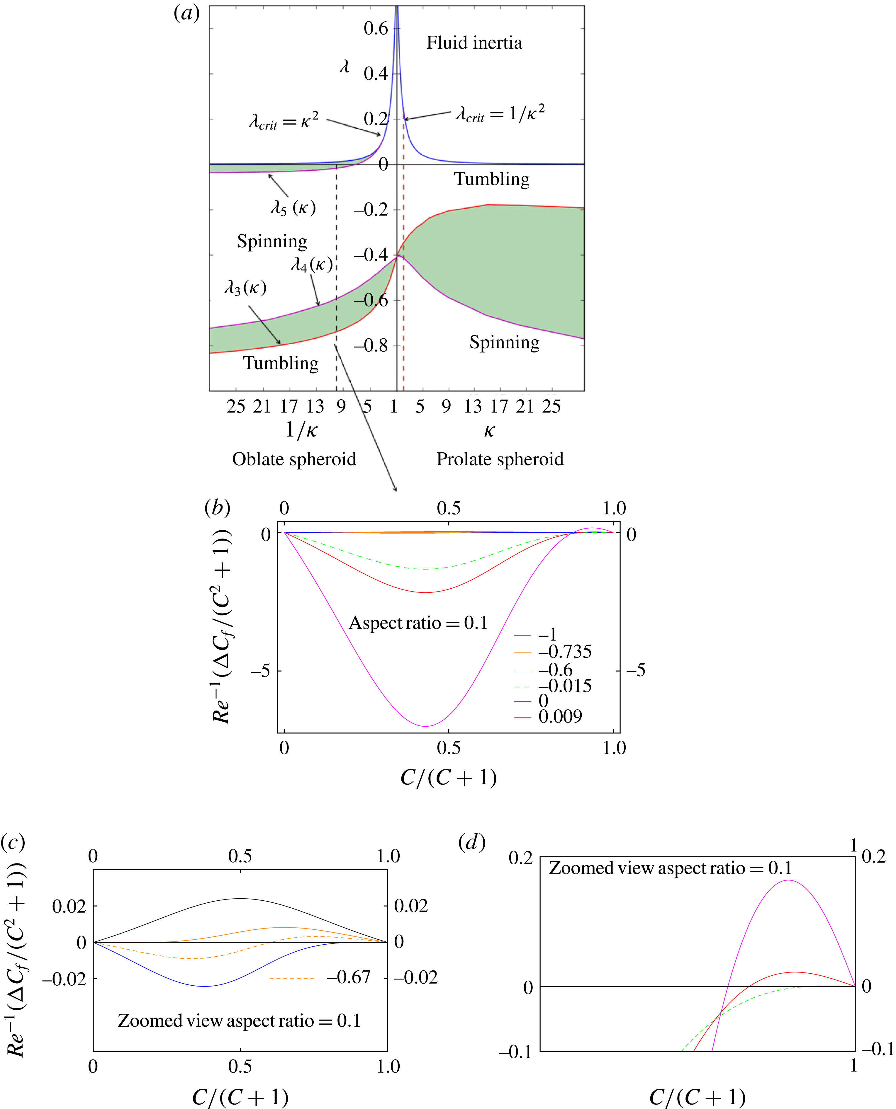
The sign of the fluid inertial drift varies in a non-trivial manner with $\unicode[STIX]{x1D706}$ for both prolate and oblate spheroids. The orbits stabilized by fluid inertia, for long times, for all $\unicode[STIX]{x1D706}$ values below the $\unicode[STIX]{x1D706}_{crit}$ curve in figure 2, are indicated in figure 6(a). For a prolate spheroid of any aspect ratio in solid-body rotation ( $\unicode[STIX]{x1D706}=-1$ ), the orbital drift is negative for all values of $C$ and the spheroid drifts towards the spinning orbit. This is expected because in solid-body rotation, the pressure gradient set up by the base state inertial forces results in a radially inward buoyancy force, which stabilizes the spinning orbit. The spinning orbit continues to be the stable orbit for all $\unicode[STIX]{x1D706}$ values less than a particular $\unicode[STIX]{x1D706}$ that is a function of the aspect ratio. This latter threshold is denoted by $\unicode[STIX]{x1D706}_{3}(\unicode[STIX]{x1D705})\;({<}0)$ and is indicated by the magenta curve in the fourth quadrant in figure 6(a). At $\unicode[STIX]{x1D706}=\unicode[STIX]{x1D706}_{3}$ , a repeller emerges from the tumbling orbit, splitting the orientation space on each unit hemisphere, for larger $\unicode[STIX]{x1D706}$ values, into two distinct basins of attraction, with the attractors being the tumbling and the spinning orbits. The repeller moves towards the spinning orbit with increasing $\unicode[STIX]{x1D706}$ , eventually merging with it at a second $\unicode[STIX]{x1D706}$ denoted by $\unicode[STIX]{x1D706}_{4}(\unicode[STIX]{x1D705})$ ( ${<}0$ and indicated by the red curve in the fourth quadrant in figure 6 a). The shaded region in figure 6(a) indicates the ( $\unicode[STIX]{x1D706},\unicode[STIX]{x1D705}$ ) combinations for which the fluid inertial drift changes sign across a certain Jeffery orbit (the repeller), leading to two distinct basins of attraction. On either side of this region, that is for $\unicode[STIX]{x1D706}$ values in the ranges $\unicode[STIX]{x1D706}_{4}<\unicode[STIX]{x1D706}<\unicode[STIX]{x1D706}_{crit}$ and $-1<\unicode[STIX]{x1D706}<\unicode[STIX]{x1D706}_{3}$ , the tumbling and spinning orbits respectively remain the sole attractors. In figure 6(b), the orbital drift is plotted against $C/(C+1)$ for a spheroid with $\unicode[STIX]{x1D705}=2$ to illustrate the abovementioned bifurcation. The shifting of the repeller location from tumbling to spinning, as one traverses the shaded bifurcation region ( $\unicode[STIX]{x1D706}_{3}<\unicode[STIX]{x1D706}<\unicode[STIX]{x1D706}_{4}$ ) in figure 6(a), can be seen in the magnified view in figure 6(c).

An oblate spheroid drifts from any initial orientation towards the tumbling orbit for $\unicode[STIX]{x1D706}=-1$ , again driven by the buoyancy contribution associated with the ambient pressure field. However, there exist ranges of $\unicode[STIX]{x1D706}$ for which there are two distinct basins of attraction separated by a repeller on the unit hemisphere. The first range is indicated by the shaded region, bounded by the curves $\unicode[STIX]{x1D706}_{3}(\unicode[STIX]{x1D705})$ and $\unicode[STIX]{x1D706}_{4}(\unicode[STIX]{x1D705})$ , in the third quadrant in figure 7(a). Unlike the prolate spheroid, the repeller in this case first emerges from the spinning orbit at $\unicode[STIX]{x1D706}=\unicode[STIX]{x1D706}_{3}(\unicode[STIX]{x1D705})$ (red curve in the third quadrant of figure 7 a) and shifts towards the tumbling orbit with increasing $\unicode[STIX]{x1D706}$ , finally merging with it when $\unicode[STIX]{x1D706}=\unicode[STIX]{x1D706}_{4}(\unicode[STIX]{x1D705})$ (the magenta curve in the third quadrant of figure 7 a). There arises a second bifurcation for $\unicode[STIX]{x1D706}>\unicode[STIX]{x1D706}_{4}$ ( $\unicode[STIX]{x1D705}$ ), and this is confined to the region bounded between the curves $\unicode[STIX]{x1D706}=\unicode[STIX]{x1D706}_{5}(\unicode[STIX]{x1D705})$ and $\unicode[STIX]{x1D706}=\unicode[STIX]{x1D706}_{crit}$ . These two curves meet at $\unicode[STIX]{x1D705}$ of approximately $0.324$ ( $\unicode[STIX]{x1D706}=0.105$ ), so that this second bifurcation is restricted to oblate spheroids smaller than this aspect ratio. For this bifurcation, the repeller (at $C=C^{\ast }$ , say) first emerges from the tumbling orbit at $\unicode[STIX]{x1D706}=\unicode[STIX]{x1D706}_{5}$ and flattens out into increasingly thin ellipses centred around the gradient–vorticity plane as $\unicode[STIX]{x1D706}\rightarrow \unicode[STIX]{x1D706}_{crit}$ . Interestingly, at $\unicode[STIX]{x1D706}=\unicode[STIX]{x1D706}_{crit}$ , the repeller does not shrink to a point, but instead reduces to an arc of the great circle in which the gradient–vorticity plane intersects the unit sphere. This is because $C^{\ast }$ remains finite in the limit of $\unicode[STIX]{x1D705}_{eq}\rightarrow 0$ ( $\unicode[STIX]{x1D706}\rightarrow \unicode[STIX]{x1D706}_{crit}$ ), the angular extent of the arc being $\unicode[STIX]{x1D703}_{j}=\tan ^{-1}\,C^{\ast }$ (see (4.2)). In figure 7(b), the orbital drift is plotted for an aspect ratio of 0.1 to show the abovementioned bifurcations. The shifting of the repeller location in the shaded bifurcation region ( $\unicode[STIX]{x1D706}_{3}<\unicode[STIX]{x1D706}<\unicode[STIX]{x1D706}_{4}$ ) in the third quadrant of figure 7(a) is plotted in figure 7(c) and the shifting in the shaded region corresponding to $\unicode[STIX]{x1D706}>\unicode[STIX]{x1D706}_{5}$ is plotted in figure 7(d). The angular extent of the limiting repeller arc (as $\unicode[STIX]{x1D706}\rightarrow \unicode[STIX]{x1D706}_{crit}$ ) is $163^{\circ }$ for the aspect ratio of 0.1. The angular extent of the repeller arc increases from approximately $161^{\circ }$ for simple shear flow (Dabade et al. Reference Dabade, Marath and Subramanian2016) to $180^{\circ }$ (a semicircle) for $\unicode[STIX]{x1D706}=0.324$ .

Figure 7.

(a) The orbits that are stabilized at long times, due to fluid inertia, are identified for all ( $\unicode[STIX]{x1D706},\unicode[STIX]{x1D705}$ ) combinations below the $\unicode[STIX]{x1D706}_{crit}$ curve (blue). (b) The drift is plotted against $C/(C+1)$ for an oblate spheroid of aspect ratio 0.1 for various $\unicode[STIX]{x1D706}$ values. (c,d) Zoomed views of (b) to show the shifting of the repeller in the two bifurcation regions identified in (a).

7 The effect of fluid inertia on neutrally buoyant spheroids ( $Re=St$ )

The inertial drifts presented in the earlier sections apply to certain limiting scenarios. The drift in § 5 is relevant to massive spheroids that occur in gas–solid systems, whereas the drift in § 6 is relevant to hollow spheroids in an inertial ambient, both in the absence of gravity (due to the neglect of sedimentation torque; see Dabade, Marath & Subramanian Reference Dabade, Marath and Subramanian2015). In this section, we investigate the combined effect of the fluid and particle inertial drifts on the orientation of a neutrally buoyant spheroid ( $\unicode[STIX]{x1D70C}_{p}=\unicode[STIX]{x1D70C}_{f}$ , $Re=St$ ) in a planar linear flow.

The drifts given in (5.10) and (6.3) are summed up to obtain the drift for a neutrally buoyant spheroid. The orbits stabilized by the combined drift at long times are indicated in figure 8. For a prolate spheroid, irrespective of $\unicode[STIX]{x1D706}$ (provided that it lies in the interval $(-1,\unicode[STIX]{x1D706}_{crit})$ ) and $\unicode[STIX]{x1D705}$ , this is the tumbling orbit. For an oblate spheroid of a given aspect ratio, there exists a critical $\unicode[STIX]{x1D706}$ ( $\hat{\unicode[STIX]{x1D706}}_{5}(\unicode[STIX]{x1D705})$ ) below which the steady state is the spinning orbit (provided that $\unicode[STIX]{x1D706}\neq -1$ ), with $\hat{\unicode[STIX]{x1D706}}_{5}(\unicode[STIX]{x1D705})$ approaching $\unicode[STIX]{x1D706}_{crit}$ as the aspect ratio increases to approximately $0.323$ ( $\unicode[STIX]{x1D706}=0.104$ ). It should be noted that this aspect ratio where $\hat{\unicode[STIX]{x1D706}}_{5}(\unicode[STIX]{x1D705})=\unicode[STIX]{x1D706}_{crit}$ is very close the aspect ratio defined by $\unicode[STIX]{x1D706}_{5}(\unicode[STIX]{x1D705})=\unicode[STIX]{x1D706}_{crit}$ in § 6, implying that the drift due to fluid inertia dominates that due to particle inertia. For $\unicode[STIX]{x1D705}<0.323$ and $\hat{\unicode[STIX]{x1D706}}_{5}(\unicode[STIX]{x1D705})<\unicode[STIX]{x1D706}<\unicode[STIX]{x1D706}_{crit}$ , there exists a repeller, as seen in the earlier sections, and the ( $\unicode[STIX]{x1D706},\unicode[STIX]{x1D705}$ ) combinations in this range are indicated by the shaded region in figure 8. It should be noted that for a given positive $\unicode[STIX]{x1D706}$ , the minimum aspect ratio for which the bifurcation above exists is given by $\unicode[STIX]{x1D705}=\sqrt{\unicode[STIX]{x1D706}}$ . For $-0.043<\unicode[STIX]{x1D706}<0$ , there is no lower bound, and, thus, there exist non-trivial basins of attraction corresponding to both tumbling and spinning orbits for oblate spheroids of an arbitrarily small aspect ratio. It is interesting to compare figures 5(a), 7(a) and 8. If the $\unicode[STIX]{x1D706}$ values are closer to simple shear than solid-body rotation, for instance in the range $\unicode[STIX]{x1D706}_{5}(\unicode[STIX]{x1D705})<\unicode[STIX]{x1D706}<\unicode[STIX]{x1D706}_{crit}$ , the drift due to fluid inertia dominates that due to particle inertia. Thus, the bifurcation region in this range, in figure 7(a), is altered by a very small amount, as is also evident from the change in the aforementioned upper critical aspect ratio (this is consistent with the observation by Dabade et al. (Reference Dabade, Marath and Subramanian2016) that fluid inertia remains dominant for neutrally buoyant spheroids in simple shear). However, the bifurcation regions in the range $\unicode[STIX]{x1D706}_{3}(\unicode[STIX]{x1D705})<\unicode[STIX]{x1D706}<\unicode[STIX]{x1D706}_{4}(\unicode[STIX]{x1D705})$ , which exist due to the fluid inertial drift alone, vanish for neutrally buoyant spheroids, since the drift due to particle inertia tends to be stronger than the fluid inertial drift when the ambient vortical component dominates the extensional component. In the case of solid-body rotation, the drift on a neutrally buoyant spheroid is zero for both prolate and oblate spheroids, as must be the case, due to the exact compensation between the centrifugal buoyancy and the centrifugal force on the particle itself. Thus, for $\unicode[STIX]{x1D706}=-1$ , the trajectory of a neutrally buoyant spheroid is a circle with $\boldsymbol{p}\boldsymbol{\cdot }\mathbf{1}_{z}^{\prime }$ being a constant, which is determined by its initial condition.

Figure 8.

The orbits stabilized for a neutrally buoyant spheroid ( $Re=St$ ) in the $\unicode[STIX]{x1D706}{-}\unicode[STIX]{x1D705}$ plane by the combined particle and fluid inertial drifts. The shaded region for the oblate spheroid corresponds to the ( $\unicode[STIX]{x1D706},\unicode[STIX]{x1D705}$ ) combinations for which the final steady state can be either the tumbling or the spinning orbit depending on the initial spheroid orientation.

8 A multiple time scale description of inertial orientation dynamics

The orbital drifts in (5.10) and (6.3) were derived from (5.6) based on an assumption that $C$ remains constant over a given turn of the actual finite- $Re$ (or - $St$ ) trajectory that is a tight inertial spiral (an example of such a spiralling trajectory was shown in figure 3). As mentioned in § 5, for $Re$ , $St\ll 1$ , the advantage of such an approximation is that it reduces the need to numerically integrate the differential equations governing $\unicode[STIX]{x1D703}_{j}$ and $\unicode[STIX]{x1D719}_{j}$ over initial orientations spanning the entire unit sphere to the determination of $\unicode[STIX]{x0394}C_{f}$ (or $\unicode[STIX]{x0394}C_{p}$ ) as a function of $C$ alone. In § 8.1, we derive the expression for the orbital drift formally using a multiple time scale analysis, and rigorously substantiate the above physically motivated characterization of inertial effects. This also allows one to discuss the limitations of the orbital drift approximation in § 8.2, and thereby derive a better approximation for extreme aspect ratio particles (slender fibres and flat disks).

8.1 A multiple-scale-based derivation of the orbital drift approximation

The inertial drift occurs on a slow time scale ( $t_{2}\sim Re^{-1}\dot{\unicode[STIX]{x1D6FE}}^{-1}$ or $St^{-1}\dot{\unicode[STIX]{x1D6FE}}^{-1}$ ) compared with the time scale of the leading-order Stokesian convection ( $t_{1}\sim \dot{\unicode[STIX]{x1D6FE}}^{-1}$ ). The orbital coordinate of the spheroid can then be written as a two-time-scale series, $C=C_{0}(t_{1},t_{2})+Re\;(\text{or}\;St)C_{1}(t_{1},t_{2})+O(Re^{3/2}\;(\text{or}\;St^{2}))$ , where $C_{0}$ will turn out to be the orbital drift at leading order discussed above and $C_{1}$ is the fluctuation about the average. The distinction between the fast and slow time scales arises from the fact that there can be no secular growth on the $t_{1}$ scale. As is the case in this formalism (Bender & Orszag Reference Bender and Orszag1999), this is enforced by the condition that $C$ be a periodic function of $t_{1}$ , with period $T_{jeff}(=2\unicode[STIX]{x03C0}(\unicode[STIX]{x1D705}_{eq}^{2}+1)/(1-\unicode[STIX]{x1D706})\unicode[STIX]{x1D705}_{eq})$ , for $t_{2}$ fixed. We will restrict our analysis to the fluid inertial drift, although an analogous analysis holds good for the particle inertia. Denoting the right-hand side of (5.6) as $Re\,H(C,\unicode[STIX]{x1D70F};\unicode[STIX]{x1D709}_{0})$ , with $\text{d}\unicode[STIX]{x1D703}_{j}/\text{d}t$ and $\text{d}\unicode[STIX]{x1D719}_{j}/\text{d}t$ given in (6.1) and (6.2), and noting that $\unicode[STIX]{x1D70F}=(1-\unicode[STIX]{x1D706})\unicode[STIX]{x1D705}_{eq}t_{1}/(\unicode[STIX]{x1D705}_{eq}^{2}+1)$ , (5.6) can be rewritten as $\text{d}C/\text{d}t=Re\,H(C,(1-\unicode[STIX]{x1D706})\unicode[STIX]{x1D705}_{eq}t_{1}/(\unicode[STIX]{x1D705}_{eq}^{2}+1);\unicode[STIX]{x1D709}_{0})$ . By substituting the series for $C$ above and using the usual splitting of the time derivative into fast and slow components, $\text{d}/\text{d}t=(\text{d}/\text{d}t_{1})+Re(\text{d}/\text{d}t_{2})$ , as part of the multiple scale formalism (Bender & Orszag Reference Bender and Orszag1999; Subramanian & Brady Reference Subramanian and Brady2004), one obtains

(8.1) $$\begin{eqnarray}\displaystyle \frac{\text{d}C_{0}}{\text{d}t_{1}}=0 & & \displaystyle\end{eqnarray}$$

at leading order and

(8.2) $$\begin{eqnarray}\displaystyle \frac{\text{d}C_{1}}{\text{d}t_{1}}+\frac{\text{d}C_{0}}{\text{d}t_{2}}=H(C,(1-\unicode[STIX]{x1D706})\unicode[STIX]{x1D705}_{eq}t_{1}/(\unicode[STIX]{x1D705}_{eq}^{2}+1);\unicode[STIX]{x1D709}_{0}) & & \displaystyle\end{eqnarray}$$

at $O(Re)$ . The leading-order orbital drift $C_{0}$ , which is the solution to (8.1) is therefore independent of $t_{1}$ , that is, $C_{0}(t_{1},t_{2})=C_{0}(t_{2})$ . To evaluate both the dependence of $C_{0}$ on $t_{2}$ and the fluctuation $C_{1}$ , one first integrates (8.2) over the Jeffery time period (the fast time scale), and noting that the integral of the first term on the left-hand side of (8.2) evaluates to zero on account of the aforementioned secularity condition, one obtains

(8.3) $$\begin{eqnarray}\displaystyle \frac{\text{d}C_{0}}{\text{d}t_{2}} & = & \displaystyle \frac{1}{T_{jeff}}\int _{0}^{T_{jeff}}H(C_{0},(1-\unicode[STIX]{x1D706})\unicode[STIX]{x1D705}_{eq}t_{1}/(\unicode[STIX]{x1D705}_{eq}^{2}+1);\unicode[STIX]{x1D709}_{0})\,\text{d}t_{1}\nonumber\\ \displaystyle & = & \displaystyle \frac{1}{2\unicode[STIX]{x03C0}}\int _{0}^{2\unicode[STIX]{x03C0}}H(C_{0},\unicode[STIX]{x1D70F};\unicode[STIX]{x1D709}_{0})\,\text{d}\unicode[STIX]{x1D70F}=\frac{\unicode[STIX]{x0394}C_{f}}{Re\,T_{jeff}},\end{eqnarray}$$

where $\unicode[STIX]{x0394}C_{f}$ is the average change in $C$ over a Jeffery time period, which was already evaluated in (6.3). Equation (8.3) is an autonomous differential equation governing $C_{0}$ . Using (8.3) in (8.2), one obtains $C_{1}$ as

(8.4) $$\begin{eqnarray}\displaystyle C_{1}=\frac{T_{jeff}}{2\unicode[STIX]{x03C0}}\left(\int _{0}^{\unicode[STIX]{x1D70F}}H(C_{0},\unicode[STIX]{x1D70F}^{\prime };\unicode[STIX]{x1D709}_{0})\,\text{d}\unicode[STIX]{x1D70F}^{\prime }-\frac{\unicode[STIX]{x1D70F}\unicode[STIX]{x0394}C_{f}}{Re\,T_{jeff}}\right). & & \displaystyle\end{eqnarray}$$

Thus, the multiple scale analysis allows one to fit $\unicode[STIX]{x0394}C_{f}$ into a differential equation for $C$ , thereby allowing one to track the evolution of $C$ with time.

Figure 9.

The orbital coordinate $C$ as a function of time and $|\unicode[STIX]{x1D719}_{j}|$ starting from $C=10$ and $\unicode[STIX]{x1D719}_{j}=0$ for spheroids of aspect ratios 0.5 and 0.02 rotating in a simple shear flow. The calculation is based on (1) the orbital drift alone obtained from solving (8.3) (red), (2) the orbital drift together with the fluctuations (green) and (3) the $C$ obtained from numerical integration of the governing equations of $\unicode[STIX]{x1D703}_{j}$ and $\unicode[STIX]{x1D719}_{j}$ (blue). In (a) and (c), $C$ is plotted against time, and in (b) and (d), it is plotted against $|\unicode[STIX]{x1D719}_{j}|$ .

In figure 9, we have plotted the $C$ coordinate for neutrally buoyant spheroids ( $Re=St$ ) of two different aspect ratios, rotating in a simple shear flow ( $\unicode[STIX]{x1D705}=\unicode[STIX]{x1D705}_{eq}$ ), as a function of time as well as $\unicode[STIX]{x1D719}_{j}$ , starting from $(C=10,\unicode[STIX]{x1D70F}=\unicode[STIX]{x03C0}/2~(\unicode[STIX]{x1D719}_{j}=0))$ , using two methods. The first method numerically integrates the total angular velocities obtained from (5.4), (5.5), (6.1) and (6.2), and then evaluates $C(t)$ using its definition (4.2) in terms of $\unicode[STIX]{x1D703}_{j}(t)$ and $\unicode[STIX]{x1D719}_{j}(t)$ . The second method uses the orbital drift obtained from the multiple-scale analysis presented above. For a neutrally buoyant spheroid, $H(C_{0},\unicode[STIX]{x1D70F}^{\prime },\unicode[STIX]{x1D709}_{0})$ would be a function of angular velocities obtained by summing that due to particle inertia given in (5.4) and (5.5) and that due to fluid inertia given in (6.1) and (6.2). The average change $\unicode[STIX]{x0394}C_{f}$ in (8.4) will be replaced by $\unicode[STIX]{x0394}C_{f}+\unicode[STIX]{x0394}C_{p}$ , with $\unicode[STIX]{x0394}C_{p}$ given in (5.10). The integral on the right-hand side of (8.4) can be evaluated analytically. Since the result of the integration (a function of $C_{0}$ , $\unicode[STIX]{x1D70F}$ and $\unicode[STIX]{x1D709}_{0}$ ) is too cumbersome, we do not present it here. To evaluate $C_{1}$ in (8.4), one needs the value of $C_{0}$ at discrete instants in time, which is obtained by numerically integrating (8.3) after accounting for the particle inertia contribution as mentioned above.

In figures 9(a) and 9(c), it can be seen that the results from the two methods compare well for oblate spheroids of different aspect ratios (the blue and green curves match almost exactly, and only one of them is therefore seen). It should be noted that the drift is a slowly varying function of time, although the degree of this variation depends on whether $C$ is plotted as a function of $t$ or $\unicode[STIX]{x1D719}_{j}$ . The latter amplifies the non-uniformity of the drift, as seen from comparing figures 9(b) and 9(d). This is due to the differing rates of change of $\unicode[STIX]{x1D719}_{j}$ with $t$ for aligned (close to the gradient–vorticity plane) and non-aligned orientations (the inclusion of the fluctuation contribution $C_{1}$ accurately captures the non-monotonic variation of the orbit constant during the aligned phases). It can be seen that for the $O(1)$ (equivalent) aspect ratio oblate spheroid in figure 9(b), the drifts in the aligned ( $\unicode[STIX]{x1D719}_{j}\approx -\unicode[STIX]{x03C0}/2,-3\unicode[STIX]{x03C0}/2$ ) and non-aligned phases ( $\unicode[STIX]{x1D719}_{j}+\unicode[STIX]{x03C0}/2,\unicode[STIX]{x1D719}_{j}+3\unicode[STIX]{x03C0}/2\,\approx O(1)$ ) are of the same order. However, for the extreme aspect ratio spheroid in figure 9(d), the dominant drift occurs in the aligned phase. This is expected and can be seen from a simple scaling analysis. The $\text{d}C/\text{d}t$ in (5.6) is $O(Re\,C)$ in the extreme (equivalent) aspect ratio limit ( $\unicode[STIX]{x1D705}_{eq}\rightarrow 0$ or $\infty$ ). The rotation is, however, non-uniform, since the spheroid spends an $O(1)$ time in the non-aligned phase and an $O(1/\unicode[STIX]{x1D705}_{eq})~(O(\unicode[STIX]{x1D705}_{eq}))$ time in the aligned phase if it is oblate (prolate). The total change in $C$ during the aligned phase, $\unicode[STIX]{x0394}C_{aligned}$ , would be $O(Re\,C/\unicode[STIX]{x1D705}_{eq})~(O(Re\,C\unicode[STIX]{x1D705}_{eq}))$ for an oblate (a prolate) spheroid, and that during the non-aligned phase, $\unicode[STIX]{x0394}C_{non\text{-}aligned}$ , would be $O(Re\,C)$ . Thus, $\unicode[STIX]{x0394}C_{non\text{-}aligned}/\unicode[STIX]{x0394}C_{aligned}$ is $O(\unicode[STIX]{x1D705}_{eq})~(O(1/\unicode[STIX]{x1D705}_{eq}))$ for an oblate (a prolate) spheroid, making the change in $C$ much larger in the aligned phase for extreme equivalent aspect ratios. As explained earlier in § 5, the prediction from the multiple-scale analysis should eventually break down when $Re$ or $St\sim \unicode[STIX]{x1D705}_{eq}$ for an oblate spheroid. The cases plotted in figure 9 are for $Re=0.01$ , satisfying the restriction $Re<\unicode[STIX]{x1D705}_{eq}$ ( $\unicode[STIX]{x1D705}_{eq}=\unicode[STIX]{x1D705}$ for $\unicode[STIX]{x1D706}=0$ ) mentioned above, hence leading to the agreement of the numerics with the analytical predictions.

Relaxation of the above restriction, however, leads to a breakdown of the multiple-scale analysis, and, thence, the notion of a one-dimensional orbital drift. To illustrate the breakdown, in figure 10, we have plotted the evolution of $C$ for a spheroid rotating in a simple shear flow ( $\unicode[STIX]{x1D705}=\unicode[STIX]{x1D705}_{eq}$ ) for different values of $Re$ , as a function of $\unicode[STIX]{x1D719}_{j}$ , starting from $(C=10,\unicode[STIX]{x1D70F}=\unicode[STIX]{x03C0}/2~(\unicode[STIX]{x1D719}_{j}=0))$ . Panels (b,d,f) in figure 10 are zoomed views of the corresponding panels (a,c,e) near a particular aligned phase ( $\unicode[STIX]{x1D719}_{j}=-\unicode[STIX]{x03C0}/2$ ). It can be seen from the figure that the sum of the orbital drift approximation ( $C_{0}$ ) and the fluctuation ( $C_{1}$ ) fails to capture the actual variation in $C$ with increasing $Re/\unicode[STIX]{x1D705}_{eq}=\widetilde{Re}$ (it should be noted that $\unicode[STIX]{x1D705}_{eq}=\unicode[STIX]{x1D705}$ in this case). Although breakdown of the orbital drift is expected as soon as $\widetilde{Re}$ becomes of order unity, the actual breakdown only occurs when $\widetilde{Re}$ is substantially larger than 1 (see figure 10 e,f). Therefore, it is necessary to characterize the inertial drift when $\widetilde{Re}$ is of $O(1)$ or larger, and we use a boundary layer analysis to accomplish this in the next subsection.

Figure 10.

The orbital coordinate $C$ as a function of $|\unicode[STIX]{x1D719}_{j}|$ starting from $C=10$ and $\unicode[STIX]{x1D719}_{j}=0$ for a spheroid with $\unicode[STIX]{x1D705}=0.02$ in simple shear flow. The calculation is based on (1) the orbital drift alone obtained by solving (8.3) (red), (2) the orbital drift together with the fluctuations (green) and (3) the $C$ obtained from numerical integration of the governing equations of $\unicode[STIX]{x1D703}_{j}$ and $\unicode[STIX]{x1D719}_{j}$ (blue). The results from these three calculations are plotted for various $Re$ values in (a), (c) and (e). Panels (b), (d) and (f) are zoomed views of (a), (c) and (e) respectively near $\unicode[STIX]{x1D719}_{j}=-\unicode[STIX]{x03C0}/2$ .

8.2 Boundary layer analysis

In this section, we characterize the inertial drift of a spheroid for $\widetilde{Re}$ of $O(1)$ or larger. We focus on oblate spheroids since it has already been shown that there is a bifurcation in the orientation dynamics for such spheroids that, based on the orbital drift approximation, occurs at increasingly extreme aspect ratios ( $\unicode[STIX]{x1D705}_{eq}\rightarrow 0$ ; the shaded green region in figure 8). In this region, it is important therefore to develop an improved approximation in order to accurately predict the location of the repeller for small but finite $Re$ .

For an extreme aspect ratio spheroid, the dominant change in $C$ occurs during the aligned phase, and therefore a boundary layer analysis allows one to capture the variation in $C$ for $O(1)$ values of $\widetilde{Re}$ even when the inertial trajectory is not a tight spiral. To see this, one first writes the net change in $C$ as

(8.5) $$\begin{eqnarray}\displaystyle \int _{0}^{-2\unicode[STIX]{x03C0}}\frac{\text{d}C}{\text{d}\unicode[STIX]{x1D719}_{j}}\text{d}\unicode[STIX]{x1D719}_{j}=\int _{0}^{-2\unicode[STIX]{x03C0}}\frac{\displaystyle \frac{\text{d}C}{\text{d}t}}{\displaystyle \frac{\text{d}\unicode[STIX]{x1D719}_{j}}{\text{d}t}+Re\,\frac{\text{d}\unicode[STIX]{x1D719}_{j}}{\text{d}t}|_{Re}}\,\text{d}\unicode[STIX]{x1D719}_{j}, & & \displaystyle\end{eqnarray}$$

where $\text{d}\unicode[STIX]{x1D719}_{j}/\text{d}t$ and $\text{d}C/\text{d}t$ are given in (2.2) and (5.6) respectively and $\text{d}\unicode[STIX]{x1D719}_{j}/\text{d}t|_{Re}$ in (8.5) is the sum of (5.5) and (6.2). Now, (2.2) can be expressed in terms of $\unicode[STIX]{x1D705}_{eq}$ as $\dot{\unicode[STIX]{x1D719}}_{j}=-(1-\unicode[STIX]{x1D706})(\unicode[STIX]{x1D705}_{eq}^{2}\sin ^{2}\unicode[STIX]{x1D719}_{j}+\cos ^{2}\unicode[STIX]{x1D719}_{j})/(\unicode[STIX]{x1D705}_{eq}^{2}+1)$ , and, in the limit $\unicode[STIX]{x1D705}_{eq}\rightarrow 0$ (an oblate spheroid approaching a flat disk), is proportional to $\cos ^{2}\unicode[STIX]{x1D719}_{j}$ after neglecting the contribution proportional to $O(\unicode[STIX]{x1D705}_{eq}^{2})$ . In this limit, $\text{d}C/\text{d}t$ remains finite and $O(Re)$ , so the integrand in (8.5) is proportional to $1/\text{cos}^{2}\unicode[STIX]{x1D719}_{j}$ and, therefore, divergent as $1/(\unicode[STIX]{x1D719}_{j}+\unicode[STIX]{x03C0}/2)$ and $1/(\unicode[STIX]{x1D719}_{j}+3\unicode[STIX]{x03C0}/2)$ for $\unicode[STIX]{x1D719}_{j}\rightarrow -\unicode[STIX]{x03C0}/2$ and $\unicode[STIX]{x1D719}_{j}\rightarrow -3\unicode[STIX]{x03C0}/2$ respectively. These divergences suggest that the dominant contribution to the integral comes from the aligned phases corresponding to $\unicode[STIX]{x1D719}_{j}=-\unicode[STIX]{x03C0}/2$ and $-3\unicode[STIX]{x03C0}/2$ , as expected from figure 10(e). One can therefore rewrite (8.5) as

(8.6) $$\begin{eqnarray}\displaystyle \int _{0}^{-2\unicode[STIX]{x03C0}}\frac{\text{d}C}{\text{d}\unicode[STIX]{x1D719}_{j}}d\unicode[STIX]{x1D719}_{j} & = & \displaystyle \int _{0}^{-\unicode[STIX]{x03C0}}\left(\frac{\text{d}C}{\text{d}\unicode[STIX]{x1D719}_{j}}-\lim _{\unicode[STIX]{x1D719}_{j}\rightarrow -\unicode[STIX]{x03C0}/2}\frac{\text{d}C}{\text{d}\unicode[STIX]{x1D719}_{j}}\right)\,\text{d}\unicode[STIX]{x1D719}_{j}+\int _{-\unicode[STIX]{x03C0}}^{-2\unicode[STIX]{x03C0}}\left(\frac{\text{d}C}{\text{d}\unicode[STIX]{x1D719}_{j}}-\lim _{\unicode[STIX]{x1D719}_{j}\rightarrow -3\unicode[STIX]{x03C0}/2}\frac{\text{d}C}{\text{d}\unicode[STIX]{x1D719}_{j}}\right)\,\text{d}\unicode[STIX]{x1D719}_{j}\nonumber\\ \displaystyle & & \displaystyle +\,\int _{0}^{-\unicode[STIX]{x03C0}}\lim _{\unicode[STIX]{x1D719}_{j}\rightarrow -\unicode[STIX]{x03C0}/2}\frac{\text{d}C}{\text{d}\unicode[STIX]{x1D719}_{j}}\,\text{d}\unicode[STIX]{x1D719}_{j}+\int _{-\unicode[STIX]{x03C0}}^{-2\unicode[STIX]{x03C0}}\lim _{\unicode[STIX]{x1D719}_{j}\rightarrow -3\unicode[STIX]{x03C0}/2}\frac{\text{d}C}{\text{d}\unicode[STIX]{x1D719}_{j}}\,\text{d}\unicode[STIX]{x1D719}_{j},\end{eqnarray}$$

where we have isolated the divergences at $-\unicode[STIX]{x03C0}/2$ and $-3\unicode[STIX]{x03C0}/2$ . Using a rescaled coordinate defined as $\hat{\unicode[STIX]{x1D719}}=(\unicode[STIX]{x1D719}_{j}+\unicode[STIX]{x03C0}/2)/\unicode[STIX]{x1D705}_{eq}$ and $\hat{\unicode[STIX]{x1D719}}=(\unicode[STIX]{x1D719}_{j}+3\unicode[STIX]{x03C0}/2)/\unicode[STIX]{x1D705}_{eq}$ respectively for the third and fourth integrals on the right-hand side above, one can rewrite (8.6) as

(8.7) $$\begin{eqnarray}\displaystyle \int _{0}^{-2\unicode[STIX]{x03C0}}\frac{\text{d}C}{\text{d}\unicode[STIX]{x1D719}_{j}}\,\text{d}\unicode[STIX]{x1D719}_{j} & = & \displaystyle \int _{0}^{-\unicode[STIX]{x03C0}}\left(\frac{\text{d}C}{\text{d}\unicode[STIX]{x1D719}_{j}}-\lim _{\unicode[STIX]{x1D719}_{j}\rightarrow -\unicode[STIX]{x03C0}/2}\frac{\text{d}C}{\text{d}\unicode[STIX]{x1D719}_{j}}\right)\,\text{d}\unicode[STIX]{x1D719}_{j}+\int _{-\unicode[STIX]{x03C0}}^{-2\unicode[STIX]{x03C0}}\left(\frac{\text{d}C}{\text{d}\unicode[STIX]{x1D719}_{j}}-\lim _{\unicode[STIX]{x1D719}_{j}\rightarrow -3\unicode[STIX]{x03C0}/2}\frac{\text{d}C}{\text{d}\unicode[STIX]{x1D719}_{j}}\right)\text{d}\unicode[STIX]{x1D719}_{j}\nonumber\\ \displaystyle & & \displaystyle +\,2\int _{\unicode[STIX]{x03C0}/2\unicode[STIX]{x1D705}_{eq}}^{-\unicode[STIX]{x03C0}/2\unicode[STIX]{x1D705}_{eq}}\frac{\text{d}C}{\text{d}\hat{\unicode[STIX]{x1D719}}}\,\text{d}\hat{\unicode[STIX]{x1D719}}.\end{eqnarray}$$

On further rewriting the above equation, one obtains

(8.8) $$\begin{eqnarray}\displaystyle \int _{0}^{-2\unicode[STIX]{x03C0}}\frac{\text{d}C}{\text{d}\unicode[STIX]{x1D719}_{j}}\,\text{d}\unicode[STIX]{x1D719}_{j} & = & \displaystyle \int _{0}^{-\unicode[STIX]{x03C0}}\left(\frac{\text{d}C}{\text{d}\unicode[STIX]{x1D719}_{j}}-\lim _{\unicode[STIX]{x1D719}_{j}\rightarrow -\unicode[STIX]{x03C0}/2}\frac{\text{d}C}{\text{d}\unicode[STIX]{x1D719}_{j}}\right)\,\text{d}\unicode[STIX]{x1D719}_{j}+\int _{-\unicode[STIX]{x03C0}}^{-2\unicode[STIX]{x03C0}}\left(\frac{\text{d}C}{\text{d}\unicode[STIX]{x1D719}_{j}}-\lim _{\unicode[STIX]{x1D719}_{j}\rightarrow -3\unicode[STIX]{x03C0}/2}\frac{\text{d}C}{\text{d}\unicode[STIX]{x1D719}_{j}}\right)\,\text{d}\unicode[STIX]{x1D719}_{j}\nonumber\\ \displaystyle & & \displaystyle +\,2\int _{\infty }^{-\infty }\frac{\text{d}C}{\text{d}\hat{\unicode[STIX]{x1D719}}}\,\text{d}\hat{\unicode[STIX]{x1D719}}-2\,\int _{\infty }^{\unicode[STIX]{x03C0}/2\unicode[STIX]{x1D705}_{eq}}\frac{\text{d}C}{\text{d}\hat{\unicode[STIX]{x1D719}}}\,\text{d}\hat{\unicode[STIX]{x1D719}}-2\int _{-\unicode[STIX]{x03C0}/2\unicode[STIX]{x1D705}_{eq}}^{-\infty }\frac{\text{d}C}{\text{d}\hat{\unicode[STIX]{x1D719}}}\,\text{d}\hat{\unicode[STIX]{x1D719}},\end{eqnarray}$$

where we have further accounted for the identity of the two aligned-phase integrals. Now, $\text{d}C/\text{d}\hat{\unicode[STIX]{x1D719}}$ is given by

(8.9) $$\begin{eqnarray}\displaystyle \frac{\text{d}C}{\text{d}\hat{\unicode[STIX]{x1D719}}}=\unicode[STIX]{x1D705}_{eq}\left.\frac{\displaystyle \frac{\text{d}C}{\text{d}t}}{\displaystyle \frac{\text{d}\unicode[STIX]{x1D719}_{j}}{\text{d}t}+Re\,\left.\frac{\text{d}\unicode[STIX]{x1D719}_{j}}{\text{d}t}\right|_{Re}}\right|_{\lim _{\unicode[STIX]{x1D705}_{eq}\rightarrow 0}}=\frac{\displaystyle C\,\widetilde{Re}\,\widetilde{F}-C\,\widetilde{Re}\,\widetilde{G}\frac{\hat{\unicode[STIX]{x1D719}}^{2}}{1+\hat{\unicode[STIX]{x1D719}}^{2}}}{-(1+\hat{\unicode[STIX]{x1D719}}^{2})(1-\unicode[STIX]{x1D706})-\widetilde{Re}\,\widetilde{G}\,\hat{\unicode[STIX]{x1D719}}}, & & \displaystyle\end{eqnarray}$$

where

(8.10) $$\begin{eqnarray}\displaystyle \widetilde{F} & = & \displaystyle \lim _{\unicode[STIX]{x1D706}\rightarrow 1/\unicode[STIX]{x1D705}^{2}}\left(F_{1}^{f}+F_{1}^{p}-F_{2}^{f}-F_{2}^{p}+(F_{3}^{f}+F_{3}^{p}+2(F_{5}^{f}+F_{5}^{p}))\frac{(1+\hat{\unicode[STIX]{x1D719}}^{2}-C^{2})}{(1+\hat{\unicode[STIX]{x1D719}}^{2}+C^{2})}+F_{4}^{f}+F_{4}^{p}\right)\nonumber\\ \displaystyle & & \displaystyle\end{eqnarray}$$

and

(8.11) $$\begin{eqnarray}\displaystyle \widetilde{G}=\lim _{\unicode[STIX]{x1D706}\rightarrow 1/\unicode[STIX]{x1D705}^{2}}\left(G_{1}^{f}+G_{1}^{p}+(G_{2}^{f}+G_{2}^{p}-G_{4}^{f}-G_{4}^{p})\frac{(1+\hat{\unicode[STIX]{x1D719}}^{2}-C^{2})}{(1+\hat{\unicode[STIX]{x1D719}}^{2}+C^{2})}-G_{3}^{f}-G_{3}^{p}\right), & & \displaystyle\end{eqnarray}$$

where the $F^{f(p)}$ and $G^{f(p)}$ terms are defined in appendix B. Noting that in the limit of $\unicode[STIX]{x1D705}_{eq}\rightarrow 0$ , $\hat{\unicode[STIX]{x1D719}}$ is large in the last two integrals on the right-hand side of (8.8), one can use (8.9) to write down the integrand of these integrals as

(8.12) $$\begin{eqnarray}\displaystyle \frac{\text{d}C}{\text{d}\hat{\unicode[STIX]{x1D719}}}=\frac{C\widetilde{Re}\widetilde{F}-C\widetilde{Re}\widetilde{G}}{\hat{\unicode[STIX]{x1D719}}^{2}(\unicode[STIX]{x1D706}-1)}, & & \displaystyle\end{eqnarray}$$

which can be solved to obtain $C=\exp (-\widetilde{Re}(\widetilde{F}-\widetilde{G})/\hat{\unicode[STIX]{x1D719}}(\unicode[STIX]{x1D706}-1))$ . On substituting the aforementioned expression for $C$ in the last two integrals in (8.8), one finds that the sum of these integrals (corresponding to the non-aligned phase) only contributes at $O(\unicode[STIX]{x1D705}_{eq})$ . The first two integrals on the right-hand side of (8.8) are obtained by subtracting the divergent terms associated with them and hence are smaller than the leading-order contribution coming from the third integral. Defining the total change in $C$ at leading order over one rotation as $2\unicode[STIX]{x0394}C_{jump}$ , one obtains $\unicode[STIX]{x0394}C_{jump}$ ,

(8.13) $$\begin{eqnarray}\displaystyle \unicode[STIX]{x0394}C_{jump}=\int _{\infty }^{-\infty }\frac{\text{d}C}{\text{d}\hat{\unicode[STIX]{x1D719}}}\,\text{d}\hat{\unicode[STIX]{x1D719}}. & & \displaystyle\end{eqnarray}$$

The jump in $C$ above is obtained by evaluating the integral in (8.13), which is carried out by numerically integrating (8.9) from $\hat{\unicode[STIX]{x1D719}}=\infty$ (a large positive value) to $\hat{\unicode[STIX]{x1D719}}=-\infty$ (a large negative value). This jump is plotted against the rescaled coordinate in figure 11 for a spheroid in a simple shear flow ( $Re=0.15$ ; $\unicode[STIX]{x1D705}=0.02$ , $\widetilde{Re}=7.5$ ). This jump (green) agrees with the total change in $C$ (blue curve) near the aligned phase, obtained from numerically solving the differential equations for the angular coordinates; in contrast, the orbital drift approximation (red) breaks down for these parameters.

Figure 11.

The orbital coordinate, during a particular aligned phase, is plotted against the rescaled boundary layer variable for a spheroid of $\unicode[STIX]{x1D705}=0.2$ in simple shear flow at $Re=0.15$ . The orbital drift approximation (8.3), the result of numerical integration ((5.6), including both the particle and the fluid inertial contribution) and the prediction from the boundary layer analysis (8.13) are shown in red, blue and green respectively.

The bifurcation region in the ( $\unicode[STIX]{x1D706},\unicode[STIX]{x1D705}$ ) plane shown in figure 8 was estimated on the basis of the orbital drift approximation. As seen above, the orbital drift need not be a good approximation to the numerics for $O(1)\widetilde{Re}$ or larger. In such cases, one would want to check the actual repeller location with that predicted by the orbital drift approximation. In figure 12, we have shown the shift in the repeller location, as a function of $\unicode[STIX]{x1D705}$ , for two values of $Re$ (0.1 and 0.3) in three planar linear flows. The repeller location is the critical $C$ ( $C^{\ast }$ ) at which the orbital drift changes sign. The solid lines are $C^{\ast }$ predictions based on numerically integrating the angular velocity of the spheroid at different $Re$ values. The green dots are $C^{\ast }$ predictions from the orbital drift approximation. For small $\widetilde{R}e$ ( $Re/\unicode[STIX]{x1D705}_{eq}\ll 1$ ; note that for a given $\unicode[STIX]{x1D706}$ , $\unicode[STIX]{x1D705}_{eq}$ increases with increasing $\unicode[STIX]{x1D705}$ ), it is evident from figure 8 that the $C^{\ast }$ prediction based on the orbital drift approximation agrees well with the results of the numerical integration. For larger $\widetilde{Re}$ (for a given $\unicode[STIX]{x1D706}$ , large $\widetilde{Re}$ implies $\unicode[STIX]{x1D705}_{eq}\rightarrow 0$ or $\unicode[STIX]{x1D705}\rightarrow \sqrt{\unicode[STIX]{x1D706}}$ ), the orbital drift approximation breaks down and the prediction from the numerical integration asymptotes to that from the boundary layer analysis mentioned above (shown as solid circles connected by dashed lines). The maximum $\widetilde{Re}$ corresponding to the smallest aspect ratio in each of the plots in figure 12 is given in the legend. It is clear from figure 12 that the orbital drift approximation together with the boundary layer analysis allows one to predict the repeller location with reasonable accuracy down to an $O(1)~\widetilde{Re}$ .

For a given $Re$ and $\unicode[STIX]{x1D706}$ , with decreasing $\unicode[STIX]{x1D705}$ , the denominator of the right-hand side of (8.9) becomes zero, and $\text{d}C/\text{d}\hat{\unicode[STIX]{x1D719}}$ diverges at a critical $\hat{\unicode[STIX]{x1D719}}$ below a critical aspect ratio (say $\unicode[STIX]{x1D705}_{FG}$ ). For oblate spheroids with $\unicode[STIX]{x1D705}<\unicode[STIX]{x1D705}_{FG}$ , there are fixed points on the flow-gradient plane, and a spheroid starting at $C>C^{\ast }(\unicode[STIX]{x1D705})$ ceases to rotate and eventually aligns with one of the stable fixed points. As discussed in § 4, in the Stokes limit, the fixed points exist on the flow-gradient plane for an oblate spheroid with $\unicode[STIX]{x1D705}<\sqrt{\unicode[STIX]{x1D706}}$ . The critical aspect ratio with inertia, $\unicode[STIX]{x1D705}_{FG}$ , is greater than $\sqrt{\unicode[STIX]{x1D706}}$ , for all positive $\unicode[STIX]{x1D706}$ values. This emergence of fixed points on the flow-gradient plane occurs for prolate spheroids as well, with $\unicode[STIX]{x1D705}_{FG}$ being less than the Stokesian value of $1/\sqrt{\unicode[STIX]{x1D706}}$ ; prolate spheroids with $\unicode[STIX]{x1D705}$ greater than this value experience an arrest of rotation. It should be noted that for a slender fibre in simple shear flow, Subramanian & Koch (Reference Subramanian and Koch2005) have already pointed out that fluid inertia arrests the rotation at a critical aspect ratio. For the ( $\unicode[STIX]{x1D706},Re$ ) combinations in figure 12, the values of $\unicode[STIX]{x1D705}_{FG}(\unicode[STIX]{x1D706},Re)$ are given by $\unicode[STIX]{x1D705}_{FG}(0,0.1)=0.01$ , $\unicode[STIX]{x1D705}_{FG}(0,0.3)=0.02$ , $\unicode[STIX]{x1D705}_{FG}(0.00009,0.1)=0.0137$ , $\unicode[STIX]{x1D705}_{FG}(0.00009,0.3)=0.031$ , $\unicode[STIX]{x1D705}_{FG}(0.0025,0.1)=0.051$ and $\unicode[STIX]{x1D705}_{FG}(0.0025,0.3)=0.058$ . Finally, it is worth mentioning that there is a rather complicated sequence of bifurcations within an $O(Re^{2})$ neighbourhood of the critical curve (for both prolate and oblate spheroids), and the resulting transitions in orientation dynamics cannot be captured within a one-dimensional orbit-constant-based interpretation. This will be reported in detail in a future article.

Figure 12.

The repeller location $C^{\ast }$ is plotted against the aspect ratio for two values of $Re$ ( $Re=0.1$ and $0.3$ ) for hyperbolic planar linear flows with (a) $\unicode[STIX]{x1D706}=0$ , (b) $\unicode[STIX]{x1D706}=0.00009$ and (c) $\unicode[STIX]{x1D706}=0.0025$ . The maximum $\widetilde{Re}$ in each of the cases is (a) 15, (b) 12.97 and (c) 21.04.

9 Effect of Brownian motion: the tumbling–spinning phase diagrams

In previous sections, it was shown that the combined effect of fluid and particle inertia uniquely determines the long-time orientation dynamics of a neutrally buoyant spheroid for a majority of ( $\unicode[STIX]{x1D706},\unicode[STIX]{x1D705}$ ) pairs below the $\unicode[STIX]{x1D706}_{crit}$ curve (see figure 8). For ( $\unicode[STIX]{x1D706},\unicode[STIX]{x1D705}$ ) pairs corresponding to the shaded region immediately below the $\unicode[STIX]{x1D706}_{crit}$ curve, however, the final spheroid orientation is not unique. As first argued by Dabade et al. (Reference Dabade, Marath and Subramanian2016) and Marath et al. (Reference Marath, Dwivedi and Subramanian2017) in the context of simple shear, one needs a stochastic orientational decorrelation mechanism, either hydrodynamic or non-hydrodynamic, for a unique orientation distribution in this region. For simple shear flow ( $\unicode[STIX]{x1D706}=0$ ), the absence of a unique steady state in the deterministic limit occurs for aspect ratios less than 0.14. In Dabade et al. (Reference Dabade, Marath and Subramanian2016), for this case, weak rotary Brownian motion (thermal orientation fluctuations) was considered as a canonical example of such an orientation decorrelation mechanism, and the unique distribution stabilized by the combined effect of inertia and Brownian motion was determined. Interestingly, as shown by Marath et al. (Reference Marath, Dwivedi and Subramanian2017), the one-dimensional reduced description in terms of the orbit constant alone, which results from the orbital drift interpretation, implies that the unique steady-state distribution must be of the Boltzmann form. The potential in the Boltzmann exponential may then be used to provide a ‘thermodynamic’ interpretation of the spheroid orientation dynamics in the presence of both inertia and Brownian motion. Interestingly, this leads to the identification of a tumbling–spinning coexistence envelope in $C$ – $\unicode[STIX]{x1D705}$ – $Re\,Pe_{r}$ space, where one expects hysteretic dynamics starting from a general initial orientation distribution; one of the signatures of this hysteresis is a multivalued viscosity at a given shear rate.

As explained by Marath et al. (Reference Marath, Dwivedi and Subramanian2017), the aforementioned hysteresis associated with the tumbling–spinning transition is analogous to that associated with the well-known coil–stretch transition (De Gennes Reference De Gennes1974; Hinch Reference Hinch1974) of high-molecular-weight polymers in an extensional flow. In the latter case, one expects the coexistence of polymer molecules in the coiled and stretched states over an intermediate range of Deborah numbers ( $De=\dot{\unicode[STIX]{x1D6FE}}\unicode[STIX]{x1D70F}_{v}$ , where $\unicode[STIX]{x1D70F}_{v}$ is the intrinsic relaxation time scale of the underlying microstructure). The coil–stretch hysteresis has since been confirmed in single-molecule experiments (Schroeder et al. Reference Schroeder, Babcock, Shaqfeh and Chu2003; Shaqfeh Reference Shaqfeh2005). Apart from interpreting the coil–stretch transition as a first-order transition in a reduced configuration space, involving only the mean polymer extension as the coarse-grained variable, De Gennes also predicted that the transition would progressively ‘soften’ with the addition of vorticity, and the sharp distinction between the coiled and stretched states would eventually vanish for simple shear flow. Following the original experiment that verified the sharp transition that occurs in planar extension (Schroeder et al. Reference Schroeder, Babcock, Shaqfeh and Chu2003), there have been a large number of experimental and numerical studies, primarily by Shaqfeh and coworkers, with the aim of understanding the dynamics of polymer molecules in planar linear flows with differing amounts of extension and vorticity (Babcock et al. Reference Babcock, Teixeira, Hur, Shaqfeh and Chu2003; Schroeder et al. Reference Schroeder, Teixeira, Shaqfeh and Chu2005; Shaqfeh Reference Shaqfeh2005; Hoffman & Shaqfeh Reference Hoffman and Shaqfeh2007; Lee et al. Reference Lee, Shaqfeh and Muller2007b ); these studies have helped to confirm De Genne’s original predictions. For spheroidal suspensions, as mentioned above, Dabade et al. (Reference Dabade, Marath and Subramanian2016) and Marath et al. (Reference Marath, Dwivedi and Subramanian2017) provided an interpretation of the orientation dynamics analogous to the polymeric case, and identified a first-order transition between the tumbling (large- $C$ ) and spinning (small- $C$ ) states for an inertial spheroid in simple shear flow. In this section, along lines similar to those of Shaqfeh and coworkers above, we examine the effect of an added extension or vorticity (corresponding to non-zero $\unicode[STIX]{x1D706}$ values) on the tumbling–spinning transition in simple shear flow ( $\unicode[STIX]{x1D706}=0$ ). It is thereby shown that the coexistence region rapidly shrinks in extent on either side of simple shear.

With the addition of rotary Brownian motion, the spheroid orientation vector, $\boldsymbol{p}$ , becomes a random variable, and the orientation distribution, $\unicode[STIX]{x1D6FA}(\boldsymbol{p},t)$ , is then governed by a convection–diffusion equation, given by

(9.1) $$\begin{eqnarray}\frac{\unicode[STIX]{x2202}\unicode[STIX]{x1D6FA}}{\unicode[STIX]{x2202}t}+\unicode[STIX]{x1D735}_{\boldsymbol{p}}\boldsymbol{\cdot }[(\dot{\boldsymbol{p}}_{jeff}+Re\,\dot{\boldsymbol{p}}_{i})\unicode[STIX]{x1D6FA}]=\frac{1}{Pe_{r}}\unicode[STIX]{x1D6FB}_{\boldsymbol{p}}^{2}\unicode[STIX]{x1D6FA}.\end{eqnarray}$$

In (9.1), $Pe_{r}$ is the rotary Péclet number, defined as $Pe_{r}=\dot{\unicode[STIX]{x1D6FE}}/D_{r}$ , where $D_{r}$ is the rotary diffusivity. The term on the right-hand side of (9.1) captures the effect of Brownian motion on the orientation distribution. The convection term on the left-hand side is made up of two contributions. The first one is the convection due to the angular velocity at leading order, denoted by $\dot{\boldsymbol{p}}_{jeff}$ ( $\unicode[STIX]{x1D734}_{jeff}\wedge \boldsymbol{p}$ ), and the second is the convection due to the inertial correction for a neutrally buoyant spheroid ( $Re=St$ ), denoted by $\dot{\boldsymbol{p}}_{i}$ . In Einarsson et al. (Reference Einarsson, Angilella and Mehlig2014), an equation similar to (9.1) was solved numerically to understand the combined effects of particle inertia and rotary Brownian motion on the orientation distribution of a spheroid in a simple shear flow. In simple shear flow, the orientation distribution set up by particle inertia alone does not change much due to weak diffusion. However, for neutrally buoyant spheroids, as shown by Dabade et al. (Reference Dabade, Marath and Subramanian2016), even weak diffusion, acting over a long period of time, will lead to a large change in the distribution for spheroids in the range of aspect ratios ( $0<\unicode[STIX]{x1D705}<0.14$ for simple shear) where inertia alone leads to a bistable scenario. This large change in distribution would be manifested as an $O(1)$ change in the intrinsic viscosity of a dilute suspension of such spheroids.

In orbital coordinates, $\dot{\boldsymbol{p}}_{jeff}$ takes the form $h_{\unicode[STIX]{x1D70F}}(1-\unicode[STIX]{x1D706})\unicode[STIX]{x1D705}_{eq}/(\unicode[STIX]{x1D705}_{eq}^{2}+1)$ $\hat{\unicode[STIX]{x1D749}}$ , where $\hat{\unicode[STIX]{x1D749}}$ is the unit vector tangent to a Jeffery orbit (for a given $C$ ) and $h_{\unicode[STIX]{x1D70F}}$ is the metric factor corresponding to the $\unicode[STIX]{x1D70F}$ coordinate (see appendix D). The convection due to the inertial correction $\dot{\boldsymbol{p}}_{i}$ takes the form $u_{iC}\hat{\boldsymbol{C}}+u_{i\unicode[STIX]{x1D70F}}\hat{\unicode[STIX]{x1D749}}$ , where $\hat{\boldsymbol{C}}$ is the same as $\hat{\unicode[STIX]{x1D73D}}_{\boldsymbol{j}}$ (see appendix D); the term proportional to $\hat{\boldsymbol{C}}$ is responsible for the drift across orbits. There are two time scales in the drift–diffusion problem as governed by (9.1). These are the fast time scale over which the distribution is convected by $\dot{\boldsymbol{p}}_{jeff}$ , and the slow time scale over which the inertial drift and the Brownian motion affect the orientation distribution along a coordinate ‘orthogonal’ to the Stokesian convection. The convection–diffusion equation in (9.1) can be solved approximately, in the limit $Re\ll 1$ , $Pe_{r}\gg 1$ ( $Re\,Pe_{r}$ being arbitrary), the limit implying that the two time scales above are disparate. Defining the fast and slow time scales as $t_{1}=t$ and $t_{2}=Re\,t$ , we use the ansatz $\unicode[STIX]{x1D6FA}(C,\unicode[STIX]{x1D70F},t_{1},t_{2})=f(C,t_{2})g(C,\unicode[STIX]{x1D70F},t_{1})$ to solve (9.1), where $f$ and $g$ are the distributions across and along the Jeffery orbits respectively (Dabade et al. Reference Dabade, Marath and Subramanian2016; Marath et al. Reference Marath, Dwivedi and Subramanian2017).

It turns out that $\dot{\boldsymbol{p}}_{jeff}$ in (9.1) rapidly sets up the steady distribution along the Jeffery orbits in the presence of a tiny polydispersity in the aspect ratio on a diffusive time scale, with the diffusivity being proportional to the variance of the aspect ratio distribution (the strictly monodisperse limit leads to an indeterminacy even for the evolution along an orbit; see Okagawa, Cox & Mason (Reference Okagawa, Cox and Mason1973), Ennis, Okagawa & Mason (Reference Ennis, Okagawa and Mason1978), Ivanov, Van de Ven & Mason (Reference Ivanov, Van de Ven and Mason1982) and Marath et al. (Reference Marath, Dwivedi and Subramanian2017)). The steady-state distribution of phase angles takes the form $g(C,\unicode[STIX]{x1D70F})=1/(h_{c}h_{\unicode[STIX]{x1D70F}}\sin \unicode[STIX]{x1D6FC})$ , where $h_{C}$ is the metric factor of the $C$ coordinate and $\unicode[STIX]{x1D6FC}$ is the angle between the unit vectors $\hat{\boldsymbol{C}}$ and $\hat{\unicode[STIX]{x1D749}}$ (see appendix D); on this time scale, the distribution across orbits remains unaltered from its initial form.

Over much longer times, the inertial drift and Brownian couples set up the distribution across Jeffery orbits, and it can be shown that (Marath et al. Reference Marath, Dwivedi and Subramanian2017) the equation governing $f(C,t_{2})$ is

(9.2) $$\begin{eqnarray}\frac{\unicode[STIX]{x2202}f}{\unicode[STIX]{x2202}t_{2}}+\frac{1}{Re}\frac{\unicode[STIX]{x2202}}{\unicode[STIX]{x2202}C}\left[\left(Re\unicode[STIX]{x0394}C_{i}-\frac{\unicode[STIX]{x1D712}_{2}}{2Pe_{r}C}\right)f\right]=\frac{1}{Re\,Pe_{r}}\frac{\unicode[STIX]{x2202}}{\unicode[STIX]{x2202}C}\left(\frac{\unicode[STIX]{x1D712}_{1}}{2}\frac{\unicode[STIX]{x2202}f}{\unicode[STIX]{x2202}C}\right),\end{eqnarray}$$

where

(9.3) $$\begin{eqnarray}\displaystyle \left.\begin{array}{@{}rcl@{}}\unicode[STIX]{x1D712}_{1}(C;\unicode[STIX]{x1D705}_{eq})\ & =\ & \displaystyle \left(\frac{\unicode[STIX]{x1D705}_{eq}^{2}+1}{\unicode[STIX]{x1D705}_{eq}^{2}}+C^{2}\left(\frac{7}{2}+\frac{1}{4\unicode[STIX]{x1D705}_{eq}^{2}}+\frac{\unicode[STIX]{x1D705}_{eq}^{2}}{4}\right)+C^{4}(\unicode[STIX]{x1D705}_{eq}^{2}+1)\right),\\ \unicode[STIX]{x1D712}_{2}\ & =\ & \displaystyle \left(-\frac{\unicode[STIX]{x1D705}_{eq}^{2}+1}{\unicode[STIX]{x1D705}_{eq}^{2}}+C^{2}\left(6-\left(\frac{7}{2}+\frac{1}{4\unicode[STIX]{x1D705}_{eq}^{2}}+\frac{\unicode[STIX]{x1D705}_{eq}^{2}}{4}\right)\right)+2C^{4}(\unicode[STIX]{x1D705}_{eq}^{2}+1)\right)\end{array}\right\}\quad & & \displaystyle\end{eqnarray}$$

and $\unicode[STIX]{x0394}C_{i}=(\unicode[STIX]{x0394}C_{p}+\unicode[STIX]{x0394}C_{f})\unicode[STIX]{x1D705}_{eq}/(\unicode[STIX]{x1D705}_{eq}^{2}+1)$ , with $\unicode[STIX]{x0394}C_{p}$ and $\unicode[STIX]{x0394}C_{f}$ being given in (5.10) and (6.3). The steady-state solution of (9.2) takes the form

(9.4) $$\begin{eqnarray}f_{s}(C)=N\exp \left[-Re\,Pe_{r}\displaystyle \int ^{C}\left(\frac{\displaystyle \frac{\unicode[STIX]{x1D712}_{2}}{Re\,Pe_{r}C^{\prime }}-2\unicode[STIX]{x0394}C_{i}(C^{\prime };\unicode[STIX]{x1D705})}{\unicode[STIX]{x1D712}_{1}}\right)\text{d}C^{\prime }\right],\end{eqnarray}$$

where $N$ is the normalization constant. For ( $\unicode[STIX]{x1D706},\unicode[STIX]{x1D705}$ ) in the shaded region in figure 8, in the absence of Brownian motion, $f_{s}(C)$ would be a singular distribution consisting of two delta functions, of the form ${\mathcal{A}}_{1}\unicode[STIX]{x1D6FF}(C)+{\mathcal{A}}_{2}\unicode[STIX]{x1D6FF}(1/C)$ , with ${\mathcal{A}}_{1}$ and ${\mathcal{A}}_{2}$ being the fractions of initial spheroid orientations on the either side of the repeller on the unit hemisphere. The functional form of the distribution reflects the fact that inertia alone stabilizes the spinning and tumbling orbits for times long compared with $O(Re\dot{\unicode[STIX]{x1D6FE}}^{-1})$ . The coefficients of the aforementioned delta functions are, however, still determined by the particular initial distribution (in the Stokes limit, even the functional form of the distribution is indeterminate). For finite $Re\,Pe_{r}$ , Brownian motion sets up a unique steady-state distribution given by (9.4). In the limit $Re\,Pe_{r}\rightarrow \infty$ , (9.4) has the same structure as the aforementioned singular distribution involving delta functions, but with the ratio ${\mathcal{A}}_{1}/{\mathcal{A}}_{2}$ being independent of the initial distribution. This is because weak Brownian motion allows for an exchange of probability between the peaks of the initial-condition-dependent bimodal distribution that results for large $Re\,Pe_{r}$ . The exchange occurs via a slow barrier-hopping process across a potential barrier set up by the bidirectional inertial drift. The presence of a slow (for $Re\,Pe_{r}\rightarrow \infty$ ) thermally driven barrier-hopping process also leads to long-lived metastable states that depend on the initial orientation distribution.

Figure 13.

(a) The potential at a $Re\,Pe_{r}$ of 70 000 is plotted against $C/(C+1)$ for spheroids of various aspect ratios in a planar linear flow with $\unicode[STIX]{x1D706}=0.00009$ ; the inset shows the complete potential for $\unicode[STIX]{x1D705}=0.12$ . (b) The curve of extrema for a $Re\,Pe_{r}$ of 70 000. The circular dots represent the extrema of the potential plotted in (a). (c) The steady-state orientation distribution at a $Re\,Pe_{r}$ of 70 000 for three aspect ratios ( $\unicode[STIX]{x1D705}=0.016,0.021,0.12$ ).

It is of interest to note that the steady-state distribution across the Jeffery orbits is of the Boltzmann form. In (9.4), the factor $1/Re\,Pe_{r}$ in the exponent therefore plays the role of the temperature, and the function that multiples $1/Re\,Pe_{r}$ can be interpreted as a potential $U(C,Re\,Pe_{r},\unicode[STIX]{x1D705},\unicode[STIX]{x1D706})$ . The steady-state distribution peaks at the minima of this potential, and these peaks can therefore be interpreted as phases. This is analogous to defining the liquid and gas phases as the minima of the Gibbs free energy in the case of a one-component system in thermodynamics. As pointed out by Marath et al. (Reference Marath, Dwivedi and Subramanian2017), in the specific context of simple shear, a closer analogy exists with respect to the well-known coil–stretch transition in the polymer physics literature (De Gennes Reference De Gennes1974; Hinch Reference Hinch1974). In general, for a given $\unicode[STIX]{x1D706}$ and $Re\,Pe_{r}$ (above a critical value), with increasing aspect ratio, the nature of the potential changes from a single-well structure peaked close to tumbling ( $C=\infty$ ), to a double-well structure, and eventually again to a single-well structure peaked close to spinning ( $C=0$ ). To illustrate this transition, we have plotted the potential for $\unicode[STIX]{x1D706}=0.00009$ , $Re\,Pe_{r}=70\,000$ , and for various aspect ratios, in figure 13(a). The potential changes as described above, with both wells having the same depth at an aspect ratio of  $0.021$ . The extrema of the potential (indicated by coloured circular dots) for various aspect ratios, given in figure 13(a), are tracked in figure 13(b). The curve connecting the extrema for $Re\,Pe_{r}=70000$ is shown there. In analogy to a thermodynamic tie line, a horizontal dashed line is drawn at $\unicode[STIX]{x1D705}=0.021$ , for which the two potential minima have the same magnitude. The small- $C$ and large- $C$ minima that it connects may be identified respectively with ‘spinning’ and ‘tumbling’ phases that coexist at the particular $\unicode[STIX]{x1D705}$ , $\unicode[STIX]{x1D706}$ and $Re\,Pe_{r}$ . One can define an isotherm consisting of three curves in figure 13(b). The first is the monotonically decreasing part of the curve of extrema, starting from the largest aspect ratio in figure 13(b) and ending at the left of the tie line; the second is the tie line itself; the third starts from the right end of the tie line and continues down to lower aspect ratios along the curve of extrema. Any point on this isotherm outside of the tie line corresponds to the $C$ at which the steady-state orientation distribution would peak for a given $Re\,Pe_{r}$ and $\unicode[STIX]{x1D705}$ . To illustrate this, in figure 13(c), we have plotted the steady-state orientation distribution for three different aspect ratios. The steady-state distribution is bimodal and both peaks have the same amplitude for a tie-line aspect ratio of 0.021. For $\unicode[STIX]{x1D705}=0.12$ , the distribution is unimodal (since the potential only has a single minimum at $C=0.076$ ), while for $\unicode[STIX]{x1D705}=0.016$ , the distribution is peaked at the deeper minimum of the corresponding potential ( $C=51.68$ ).

One can repeat the above exercise for various $Re\,Pe_{r}$ values to develop a ‘phase diagram’, as shown in figure 14(a) for $\unicode[STIX]{x1D706}=0.0009$ . The constant $Re\,Pe_{r}$ loci in figure 14(a) may again be regarded as isotherms. The tie lines now replace the intermediate non-monotonic portion in figure 14(a), resulting in a two-phase (tumbling–spinning) envelope that ends in a critical point, $(\unicode[STIX]{x1D705},C,Re\,Pe_{r},\unicode[STIX]{x1D706})\equiv (0.0665,2.31,1200,0.00009)$ , as shown in figure 14(b). Such a phase diagram, emphasizing a ‘thermodynamic’ interpretation of the orientation dynamics, has already been developed for the specific case of simple shear flow ( $\unicode[STIX]{x1D706}=0$ ) by Marath et al. (Reference Marath, Dwivedi and Subramanian2017). The isotherm corresponding to $Re\,Pe_{r}=\infty$ in figure 14(b) is defined as a piecewise linear curve made up of three segments, defined as (1) $C=0$ , when $\unicode[STIX]{x1D705}>0.0155$ , (2) $\unicode[STIX]{x1D705}=0.0155$ , when $0<C<\infty$ , and (3) $C=\infty$ , when $0.0094<\unicode[STIX]{x1D705}<0.0155$ . Therefore, in the limit of $Re\,Pe_{r}\rightarrow \infty$ , the orientation distribution discontinuously changes from a delta function localized at the spinning orbit above $\unicode[STIX]{x1D705}=0.0155$ to one localized at the tumbling orbit below $\unicode[STIX]{x1D705}=0.0155$ (this discontinuous change in the steady-state distribution nevertheless requires an infinite amount of time in the limit $Re\,Pe_{r}\rightarrow \infty$ ; see the discussion below). The phase diagram is cut off (below) at an aspect ratio of $\unicode[STIX]{x1D705}=\sqrt{0.00009}=0.0095$ , plotted as the lowest horizontal line in figure 14(b), since for smaller aspect ratios, the Stokesian trajectories are not closed and the interpretation based on averaging over Jeffery orbits breaks down. For simple shear flow ( $\unicode[STIX]{x1D706}=0$ ) analysed by Marath et al. (Reference Marath, Dwivedi and Subramanian2017), the phase diagram extends down to $\unicode[STIX]{x1D705}=0$ , with the discontinuous transition occurring at an aspect ratio of $0.0126$ in the limit of $Re\,Pe_{r}\rightarrow \infty$ .

Figure 14.

(a) The curves of extrema corresponding to different values of $Re\,Pe_{r}$ . (b) The envelope joining the tie lines for the phase diagram in (a). The red circular dot corresponds to the critical point $(\unicode[STIX]{x1D705},C,Re\,Pe_{r},\unicode[STIX]{x1D706})\equiv (0.0665,2.31,1200,0.00009)$ ; the phase diagram is cut off at $\unicode[STIX]{x1D705}=\sqrt{\unicode[STIX]{x1D706}}=0.0095$ .

Figure 15.

The tumbling–spinning phase diagrams for various values of $\unicode[STIX]{x1D706}$ . Panel (a), showing $\unicode[STIX]{x1D706}=0$ for simple shear flow is reproduced from Marath et al. (Reference Marath, Dwivedi and Subramanian2017). Panels (b–d) correspond to negative values of $\unicode[STIX]{x1D706}$ and panels (e–g) correspond to positive values of $\unicode[STIX]{x1D706}$ . The phase diagrams in (e–g) are cut off at (e) $\unicode[STIX]{x1D705}=0.0095$ , (f) $\unicode[STIX]{x1D705}=0.05$ and (g) $\unicode[STIX]{x1D705}=0.173$ .

The phase diagrams for a range of planar linear flows in the neighbourhood of simple shear are plotted in figure 15. Those for positive $\unicode[STIX]{x1D706}$ values are bounded below by $\unicode[STIX]{x1D705}=\sqrt{\unicode[STIX]{x1D706}}$ , the smallest aspect ratio at which the orbits of the spheroid are closed in the Stokes limit. It should be noted that with increasing $\unicode[STIX]{x1D706}$ (positive), the lower bound of the phase diagram, defined by $\unicode[STIX]{x1D705}=\sqrt{\unicode[STIX]{x1D706}}$ , moves upward. The largest aspect ratio at which the potential is bistable, for a given $Re\,Pe_{r}$ , also increases with increasing $\unicode[STIX]{x1D706}$ (positive). The lower bound, however, increases at a faster rate, and the net result is that the region corresponding to a bistable potential shrinks for positive $\unicode[STIX]{x1D706}$ , vanishing at a $\unicode[STIX]{x1D706}$ value of approximately 0.2. Above this particular $\unicode[STIX]{x1D706}$ , irrespective of $Re\,Pe_{r}$ and $\unicode[STIX]{x1D705}$ ( ${>}\sqrt{\unicode[STIX]{x1D706}}$ ), the potential only has a single minimum. The region of coexistence defined by the tie lines as seen in figure 14(b) also disappears at a $\unicode[STIX]{x1D706}$ value of approximately $0.2$ . It should be noted that a region of coexistence implies that there should be an aspect ratio at which the potential has two minima of equal depth, and therefore is found over a narrower range of parameters than that corresponding to a potential that is bistable. The critical aspect ratio at which the discontinuous transition from spinning to tumbling spheroids occurs (for $Re\,Pe_{r}\rightarrow \infty$ ) also increases with increasing $\unicode[STIX]{x1D706}$ . However, the rate of increase is again smaller than that of the lower bound ( $\unicode[STIX]{x1D705}=\sqrt{\unicode[STIX]{x1D706}}$ ). This discontinuous transition, therefore, ceases to exist for $\unicode[STIX]{x1D706}$ values greater than $0.042$ . In other words, for $\unicode[STIX]{x1D706}>0.042$ , the final steady-state distribution in the limit $Re\,Pe_{r}\rightarrow \infty$ would be a delta function localized at the spinning orbit. Thus, for $0.042<\unicode[STIX]{x1D706}<0.2$ , the steady-state distribution in the limit $Re\,Pe_{r}\rightarrow \infty$ (weakly Brownian limit) is different from the deterministic limit (no Brownian motion), the distribution corresponding to the latter being two delta functions, with one peaked at the spinning orbit and the other at the tumbling orbit, and the coefficients of the delta functions being determined by the initial orientation distribution.

When $\unicode[STIX]{x1D706}$ is negative, the aspect ratio bounding the bistable region from above (for a given $Re\,Pe_{r}$ ) decreases with decreasing $\unicode[STIX]{x1D706}$ , but the lower threshold remains at $\unicode[STIX]{x1D705}=0$ (the Stokesian trajectories are always closed for $\unicode[STIX]{x1D706}<0$ regardless of aspect ratio). Therefore, the region with bistable potential shrinks for negative $\unicode[STIX]{x1D706}$ and disappears earlier at a $\unicode[STIX]{x1D706}$ of approximately $-0.043$ . The region of coexistence disappears earlier at a $\unicode[STIX]{x1D706}$ of approximately $-0.005$ . The discontinuous transition (in the limit $Re\,Pe_{r}\rightarrow \infty$ ) mentioned above ceases to exist below a $\unicode[STIX]{x1D706}$ of approximately $-0.0002$ .

The coexistence region in the simple shear flow case (Marath et al. Reference Marath, Dwivedi and Subramanian2017) rapidly shrinks on either side with increasing $|\unicode[STIX]{x1D706}|$ . In the limit $Re\,Pe_{r}\rightarrow \infty$ , the discontinuous transition from spinning to tumbling occurs only for $\unicode[STIX]{x1D706}$ ranging from $-0.0002$ to $0.042$ , at a $\unicode[STIX]{x1D706}$ -dependent aspect ratio. As mentioned earlier, such a transition for simple shear flow occurs at an aspect ratio of $0.0126$ (Dabade et al. Reference Dabade, Marath and Subramanian2016). For $\unicode[STIX]{x1D706}$ outside the aforementioned range, the long-time distribution is a delta function localized at the spinning orbit.

Although we have focused on the steady-state orientation distribution above, for large $Re\,Pe_{r}$ , one might have to wait for an exceedingly long time to see the development of the steady state, especially in regions of parameter space where it is bimodal. This is because when the potential is bistable, the two minima are separated by a barrier at an intermediate maximum (see figure 13 a), and the eventual evolution to the steady state would depend on a slow barrier-hopping process driven by weak thermal fluctuations. An estimate of this time can be made using the Kramers reaction rate theory (Chandrasekhar Reference Chandrasekhar1943), and the time scale is given by $(4\unicode[STIX]{x03C0}\,Re\,Pe_{r}/\unicode[STIX]{x1D712}_{1}|_{C_{max}}(f^{\prime \prime }|_{C_{max}}\,f^{\prime \prime }|_{C_{min}})^{1/2})\text{e}^{Re\,Pe_{r}\unicode[STIX]{x0394}U}$ , where $\unicode[STIX]{x0394}U$ is the magnitude of the difference in the potential between the lowest minimum ( $C_{min}$ ) and the intermediate maximum ( $C_{max}$ ) of the bistable potential (Marath et al. Reference Marath, Dwivedi and Subramanian2017). The time scale for barrier hopping is thus proportional to the exponential of $Re\,Pe_{r}$ , which can be very large for most of the $Re\,Pe_{r}$ values in figure 15. Depending on the initial conditions, the orientation distribution of the spheroid might therefore evolve rapidly to an initial-condition-dependent quasiequilibrium (a metastable state), and the subsequent evolution to the time steady state may not occur over the duration of an experiment. The existence of such metastable distributions is therefore expected to result in a hysteresis characterizing the transition between tumbling and spinning modes. As mentioned above, the range of $\unicode[STIX]{x1D705}$ for which such a bistable potential exist shrinks with increasing $|\unicode[STIX]{x1D706}|$ , and the hysteresis is therefore most relevant to flows in the immediate neighbourhood of simple shear. An increase in the extension–vorticity imbalance, at a fixed aspect ratio, should, in principle, lead to an aspect-ratio-dependent critical flow at which the coexistence region shrinks to a point (much like simple shear flow for the coil–stretch transition; see Shaqfeh Reference Shaqfeh2005). The phase diagrams suggest that such a scenario is realized for a very small excess of vorticity ( $\unicode[STIX]{x1D706}<0$ ). The scenario on the hyperbolic side (excess extension, $\unicode[STIX]{x1D706}>0$ ) is more complex since the tumbling–spinning coexistence can only exist until $\unicode[STIX]{x1D706}=\unicode[STIX]{x1D705}^{2}$ , and the truncation of the coexistence region due to the upward movement of this line may therefore precede the appearance of a critical point (at a fixed aspect ratio).

10 Conclusions and future work

In this paper, we have analysed the effect of particle and fluid inertia on the orientation dynamics of a spheroid in a planar linear flow. The $O(St)$ correction to the leading-order angular velocity of a spheroid has already been derived by Einarsson et al. (Reference Einarsson, Angilella and Mehlig2014), but the analysis was restricted to simple shear flow ( $\unicode[STIX]{x1D706}=0$ ). With the aim of understanding the effect of particle inertia in flows with non-zero $\unicode[STIX]{x1D706}$ values, the $O(St)$ corrections are rederived in § 5 and are given in (5.4) and (5.5). The corrections, at $O(Re)$ , arising from fluid inertia are given in (6.1) and (6.2). We have used an orbital drift approximation to analyse the solution of the differential equations governing the angular coordinates, the orbital drift being defined as a change in the orbit constant, given in (4.2), per Jeffery time period. The orbital drifts for the particle and fluid inertia cases are given in (5.10) and (6.3) respectively. The orbits stabilized by particle and fluid inertia are identified in the $\unicode[STIX]{x1D706}{-}\unicode[STIX]{x1D705}$ plane in figures 4 and 5 and figures 6 and 7 respectively. The shaded regions in these figures correspond to the ( $\unicode[STIX]{x1D706},\unicode[STIX]{x1D705}$ ) combinations for which there is a repeller on the unit hemisphere that divides the orientation space into two basins of attraction, with the attractors being the tumbling and spinning orbits respectively. Typical examples of repellers are shown in figure 4(d–f). The orbits stabilized by inertia for the important case of neutrally buoyant spheroids are identified in figure 8. For the neutrally buoyant case, the bifurcation leading to both tumbling and spinning orbits as possible steady states exists only for oblate spheroids with aspect ratios less than a $\unicode[STIX]{x1D706}$ -dependent threshold that has a maximum value of $0.323$ for a planar linear flow with $\unicode[STIX]{x1D706}=0.104$ . For all inertial scenarios, other than the neutrally buoyant case, the spheroid, in addition to convecting with the ambient shear flow, will also sediment relative to it due to gravity. The role of the sedimentation-induced torque, analysed in the quiescent scenario by Dabade et al. (Reference Dabade, Marath and Subramanian2015), is neglected here. An analysis of the orientation dynamics under the combined effects of an ambient shear and gravity will be reported separately (Marath & Subramanian Reference Marath and Subramanian2017).

In recent efforts, Rosen, Lundell & Aidun (Reference Rosen, Lundell and Aidun2014) and Rosen et al. (Reference Rosen, Do-Quang, Aidun and Lundell2015a ) numerically examined the effects of both particle and fluid inertia on a force-free spheroid in a simple shear flow, and attributed the drift of a weakly inertial prolate spheroid towards the tumbling orbit to the effects of particle inertia. For a prolate spheroid of aspect ratio 4, for example, fluid inertia is thought to play a role only beyond a critical $Re$ at which a bifurcation renders both the tumbling and the log-rolling states stable. This conclusion is incorrect, and is likely to be motivated by some of the earliest efforts which erroneously concluded that the fluid inertial effects stabilize the spinning orbit (Taylor Reference Taylor1923; Saffman Reference Saffman1956; Karnis, Goldsmith & Mason Reference Karnis, Goldsmith and Mason1963). Our earlier work on simple shear flow has already shown that fluid inertia is dominant for small $Re$ , and for $O(1)$ values of the ratio $St/Re$ . Further, numerical simulations at a $Re$ of $O(1)$ (Rosen et al. Reference Rosen, Einarsson, Nordmark, Aidun, Lundell and Mehlig2015b ) were shown to be qualitatively in agreement with analytical predictions for small $Re$ (Einarsson et al. Reference Einarsson, Candelier, Lundell, Angilella and Mehlig2015; Dabade et al. Reference Dabade, Marath and Subramanian2016). Thus, one expects fluid inertia to continue to dominate particle inertia for $O(1)\;Re$ values at least up to the aforementioned bifurcation value. The present effort shows that the fluid inertia continues to remain dominant for hyperbolic planar linear flows, and for elliptic linear flows in the vicinity of simple shear. As shown in § 7 for neutrally buoyant spheroids, the bifurcation region for oblate spheroids is virtually unchanged in form relative to its estimate for $St=0$ in § 6. For $\unicode[STIX]{x1D706}$ values closer to solid-body rotation, however, the drift due to particle inertia is dominant (notwithstanding the centrifugal buoyancy contribution).

In § 9, an orientation decorrelation mechanism in the form of rotary Brownian motion was included in the analysis in order to eliminate the aforementioned possibility of multiple steady states. The steady-state orientation distribution under the combined effect of Brownian motion and inertia lends itself to an elegant thermodynamic interpretation in $C$ – $\unicode[STIX]{x1D705}$ – $Re\,Pe_{r}$ space. The transition of the distribution from a unimodal to a bimodal one has similarities to a phase transition, and the small- and large- $C$ minima of the bimodal distribution are identified with spinning and tumbling phases. The tumbling–spinning coexistence region in the $C$ – $\unicode[STIX]{x1D705}$ – $Re\,Pe_{r}$ space is identified, and it is shown that this region shrinks rapidly with increasing $|\unicode[STIX]{x1D706}|$ . That is to say, the coexistence region is maximum in extent for simple shear, and diminishes rapidly for planar linear flows on either side of simple shear (with increasing extension or vorticity). The orientation dynamics in the coexistence region is expected to have a strong hysteretic signature, with initial-condition-dependent metastable states likely to be seen in real experiments. The transition from the metastable states to the final steady states through a barrier-hopping process, when driven by thermal fluctuations alone, may take an exceedingly long time.

Any mechanism that leads to stochastic orientation fluctuations could play a role similar to rotary Brownian motion, and thereby give rise to interesting non-equilibrium transitions between different orientational states, and hysteretic dynamics. An example of this is athermal fluctuations driven by hydrodynamic interactions (Dabade et al. Reference Dabade, Marath and Subramanian2016). They differ in character from thermal orientation fluctuations in that the decorrelation is driven by large jumps in orientation triggered by pair encounters rather than a succession of small-amplitude jumps that characterize a rotary diffusion process. The governing integro-differential equation can be formally written down (as has been done in Marath et al. (Reference Marath, Dwivedi and Subramanian2017)), although lack of any detailed knowledge about the kernel related to pair hydrodynamic interaction renders a solely theoretical resolution impossible. Experimentally, this route might nevertheless be the easier one in terms of using the volume fraction as a parameter to tune the barrier-hopping times to values that are accessible in real experiments.

The bidirectional drift, and the resulting dependence of the final state on initial orientation, may also arise due to other sources of nonlinearity such as viscoelasticity. An experiment (Petrich et al. Reference Petrich, Chaouche, Koch and Cohen2000) investigating the behaviour of non-Brownian fibres suspended in an elastic fluid, under oscillatory shear, has, in fact, already demonstrated the existence of multiple steady states for the fibre orientation. At moderate strain and an $O(1)$ Deborah number (a non-dimensional number characterizing the effect of viscoelasticity given by the product of an ambient shear rate and the microstructural relaxation time), the authors find that the flow as well as the vorticity directions act as stable fixed points, and at long times, a fibre, depending on its initial orientation, will be aligned with either of the two directions (Petrich et al. Reference Petrich, Chaouche, Koch and Cohen2000). Further, a recent numerical simulation (d’Avino et al. Reference d’Avino, Hulsen, Greco and Maffettone2014) has reported that the steady-state orientation of a non-Brownian prolate spheroid of aspect ratio 4 suspended in a viscoelastic fluid, when subjected to a simple shear flow, is not unique; it is again determined by the initial orientation of the spheroid. If the fibres (or the spheroid in the simulation) were Brownian, or if the fibre (spheroid) concentration were large enough for hydrodynamic interactions to drive orientation fluctuations, a unique steady-state partitioning between the different orientation states could be achieved. One can, in principle, tune the strength of the Brownian motion independent of the viscoelasticity by altering the size of the spheroid, and, from the experimental viewpoint, it may therefore be easier to demonstrate the existence of non-equilibrium orientational order transitions found here, and in Marath et al. (Reference Marath, Dwivedi and Subramanian2017), under the combined effect of viscoelasticity and rotary Brownian motion.