A Model of Global Beverage Markets

Glyn Wittwer; Kym Anderson

doi:10.1017/jwe.2020.17

A Model of Global Beverage Markets

Published online by Cambridge University Press: 01 September 2020

Glyn Wittwer and

Kym Anderson

Show author details

Glyn Wittwer: Affiliation:
Centre of Policy Studies, Victoria University, 300 Flinders Street, Melbourne VIC 8001, Australia; e-mail: Glyn.Wittwer@vu.edu.au.
Kym Anderson*: Affiliation:
Wine Economics Research Centre, School of Economics, University of Adelaide, Adelaide SA 5005, Australia and Arndt-Corden Department of Economics, Australian National University, Canberra ACT 2600
*: e-mail: kym.anderson@adelaide.edu.au (corresponding author).

Article contents

Abstract
Introduction
Summary of the Global Beverage Model
Data Sources
Projecting the GLOBAL-BEV Model to 2025 (Business-as-Usual)
Effects of Brexit by 2025
Effects of an Extra 25% Tariff on U.S. Imports of Some EU Beverages by 2025
Conclusion
Footnotes
References

Rights & Permissions

Abstract

This article describes a new empirical model of the world's markets for alcoholic beverages and, to illustrate its usefulness, reports results from projections of those markets from 2016–2018 to 2025 under various scenarios. It not only revises and updates a model of the world's wine markets (Wittwer, Berger, and Anderson, 2003), but also adds beer and spirits so as to capture the substitutability of those beverages among consumers. The model has some of the features of an economy-wide computable general equilibrium model, with international trade linking the markets of its 44 countries and seven residual regions. It is used to simulate prospects for these markets by 2025 (business-as-usual), which points to Asia's rise. Then two alternative scenarios to 2025 are explored: one simulates the withdrawal of the United Kingdom from the European Union (EU); the other simulates the effects of the recent imposition of additional 25% tariffs on selected beverages imported by the United States from several EU member countries. Future applications of the model are discussed in the concluding section. (JEL Classifications: C53, F11, F17, Q13)

Keywords

CGE modeling changes in beverage preferences international trade in beverages premiumization of alcohol markets

Information

Type: Articles
Information: Journal of Wine Economics , Volume 15 , Issue 3 , August 2020 , pp. 330 - 354

DOI: https://doi.org/10.1017/jwe.2020.17 [Opens in a new window]
Copyright: Copyright © American Association of Wine Economists, 2020

I. Introduction

Beverage markets are continuously evolving as technologies and preferences change with population and income growth, and as producers, investors, traders, and consumers respond also to changes in pertinent policies in their own and other countries. Among the three main alcoholic beverage groups, the traditional concentration of each nation's consumers on one of them (wine, beer, or spirits) has been reducing gradually in recent decades. This has contributed to a convergence across countries toward the global average mix of alcoholic consumption, and an increase in the share of global production of each beverage that is traded internationally (Anderson, Meloni, and Swinnen, Reference Anderson, Meloni and Swinnen2018). Since the beverage facing the lowest consumer tax in each country traditionally was the dominant one, a move toward a more uniform tax per unit of alcohol in any country would add to that convergence tendency. Analysis of such market developments and possible policy reforms requires a global economic model in which the interactions between each nation's producers and consumers of these three beverages are explicitly recognized. The purpose of this article is to provide such a model, calibrate it to 2016–2018 data, and illustrate its usefulness by projecting its national and hence global markets to 2025 under various scenarios.

Projecting changes in such markets is a fraught business. Yet many participants in these markets intuitively need to do this all the time. This model does not provide predictions of what will happen, but rather a business-as-usual scenario as a baseline against which to compare alternative scenarios that one might envisage.

Section II begins by summarizing the new model of global beverage markets that builds on an earlier model of global wine markets. (Details are provided in the Appendix.) Section III provides the sources of data in the model's baseline dataset, which is calibrated to 2016–2018. Section IV draws on past trends in beverage markets to simulate prospects for these markets by 2025, as projected by the model over those eight years (our business-as-usual scenario). Sections V and VI then explore alternative scenarios to 2025. Section V simulates the withdrawal of the United Kingdom from the European Union (Brexit) to see how that is likely to affect the business-as-usual projection of the world's beverage markets by 2025. Section VI simulates the effects of the recent imposition of the additional 25% tariffs on selected beverages imported by the United States from the European Union (EU). The concluding section points to further potential applications of this model, most obviously in the area of changes to consumer taxes on beverages and the shock of the COVID-19 epidemic.

II. Summary of the Global Beverage Model

GLOBAL-BEV is a multi-product model that builds on a model of the world's wine markets (Wittwer, Berger, and Anderson, Reference Wittwer, Berger and Anderson2003). Its theory is based on that of an economy-wide computable general equilibrium (CGE) model in the ORANI school (Dixon et al., Reference Dixon, Parmenter, Sutton and Vincent1982). Within the model, wine markets have been disaggregated into four types, namely non-premium (including bulk), commercial-premium, and super-premium still wines, plus sparkling wine. Commercial-premium still wines are defined by Anderson, Nelgen, and Pinilla (Reference Anderson, Nelgen and Pinilla2017) to be those between US$2.50 and $7.50 per liter pre-tax at a country's border or wholesale. Beer and spirits are not split into regular and craft categories, because the latter still have small (albeit growing) market shares in volume terms. The world is divided into 44 individual nations, with all other countries being captured in seven composite residual regions. Each industry uses a combination of intermediate and primary inputs to produce a unit of output. Consumers demand the various beverages plus a composite product making up all other expenditures in each country. Imports and exports of all final products are possible, while winegrape inputs are considered nontradable internationally. GLOBAL-BEV includes nominal exchange rates relative to the U.S. dollar (the numeraire). Changes in a nation's nominal exchange rate will affect a producer's competitiveness in global beverage markets whenever it is transmitted through to real impacts; but if a movement in the general price level and in nominal wages exactly offset a nominal exchange rate movement, there is no change in a nation's international competitiveness.

III. Data Sources

The primary sources of data for constructing the GLOBAL-BEV model's baseline database for 2016–2018 are Anderson and Pinilla (Reference Anderson and Pinilla2020) plus Anderson (Reference Anderson2020a) for taxes on beverage consumption and imports, Holmes and Anderson (Reference Holmes and Anderson2017) for wine, beer, and spirits average consumer expenditure data, and United Nations (2019) for volume and value of international trade in beverages.

IV. Projecting the GLOBAL-BEV Model to 2025 (Business-as-Usual)

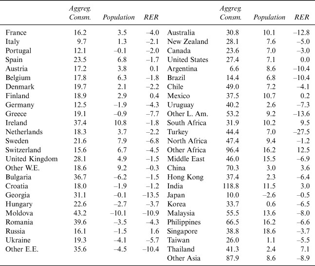
The model is projected forward to 2025 based on anticipated growth in aggregate national household consumption (a measure of real disposable income) and population together with anticipated changes in real exchange rates that are reported in Table 1, plus a number of additional assumptions concerning trends in consumer preferences, production, technologies, and capital stocks.

Table 1

Cumulative Consumption and Population Growth Rates and Changes in the Real Exchange Rate (RER) Relative to the U.S. Dollar, Business-as-Usual Scenario, 2017 to 2025 (%)

Source: Authors' compilation from projections by various international agencies.

Concerning preferences, there is assumed to be a swing towards all wine types in China, as more Chinese earn middle-class incomes. Previous modeling (Anderson and Wittwer, Reference Anderson and Wittwer2013) revealed that without such a taste swing, income growth alone would have been incapable of tracing the rapid growth in China's wine consumption (and hence imports, which over the decade to 2018 accounted for one-quarter of the growth in the value of global wine imports). For the rest of the world, the long-trend preference swings away from non-premium wines and toward commercial and super-premium wines are assumed to continue. No changes are assumed for beer and spirits preferences.

Total factor productivity is assumed to grow everywhere at 1.2% and 2.3% per year, respectively, in the grape industry and wine industries, and at 2.3% per year in the beer and spirits industries everywhere. Grape and wine industry capital are assumed to not grow net of depreciation except in China, but there is a shift in capital away from non-premium towards premium wine production, in keeping with global demand swings. China's wine production is assumed to rise by one-fifth above its 2016–2018 level by 2025, so well above its slumped 2018 level. If China's wine production was to remain at its low 2018 level, its wine imports would increase more than projected below.

This global model has supply and demand equations and hence quantities and prices for each of the grape and wine products and for beer and spirits, plus for a single composite of all other products in each country such that it has elements of an economy-wide CGE model. Grapes are assumed to be not traded internationally, but other products are both exported and imported. Each market is assumed to have cleared before any exogenously introduced shock to the baseline projection of 2025 and to find a new market-clearing outcome following each shock. The inclusion of real exchange rate variables explicitly in the model enables a distinction between price impacts as observed in local currency units from those observed in U.S. dollars. All prices are expressed in real (2017) U.S. dollar terms.

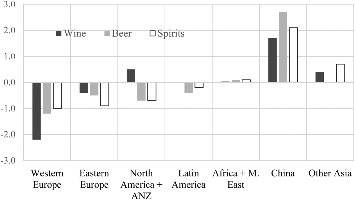
Given the above assumptions, and consistent with recent trends (Anderson, Reference Anderson2020b), the GLOBAL-BEV model projects Asia will become a substantially larger player in global beverage markets. Specifically, since Asia is currently drinking less wine and beer per capita than the rest of the world, its consumption is expected to keep rising as its economic growth continues; and while its mix of alcohols is now much closer to the world average than it was in earlier decades, the share of grape wine in that mix is still very low. That wine share is projected to increase, just as it has happened in recent decades in Western European countries that are net importers of wine: only a very small share of the latter's alcohol consumption was accounted for by wine in the early 1960s, but by 2016–2018 wine accounted for around one-third of their alcohol consumption. The extent of that preference shift toward wine in Asia is minor by comparison, with its consumption projected to grow only a little faster for wine than for beer and spirits. As a result, by 2025, China's shares of global beverage consumption are projected to be 1.7 percentage points higher for wine, 2.7 points higher for beer, and 2.1 points higher for spirits than in 2016–2018. The shares for the rest of Asia are up too for both wine and spirits, but by less than 1 percentage point. Africa also is projected to raise its share of global alcohol consumption, but only very slightly. By contrast, shares of Western Europe are projected to be much lower in 2025 than in 2016–2018 (Figure 1). Regional shares of world exports do not alter greatly over the projection period, but shares of world imports change non-trivially (see below).

Figure 1

Projected Changes in Regional Shares of the Global Volume of Consumption of Wine, Beer and Spirits, 2016–2018 to 2025 (percentage points)

Source: Authors' model projections, business-as-usual.

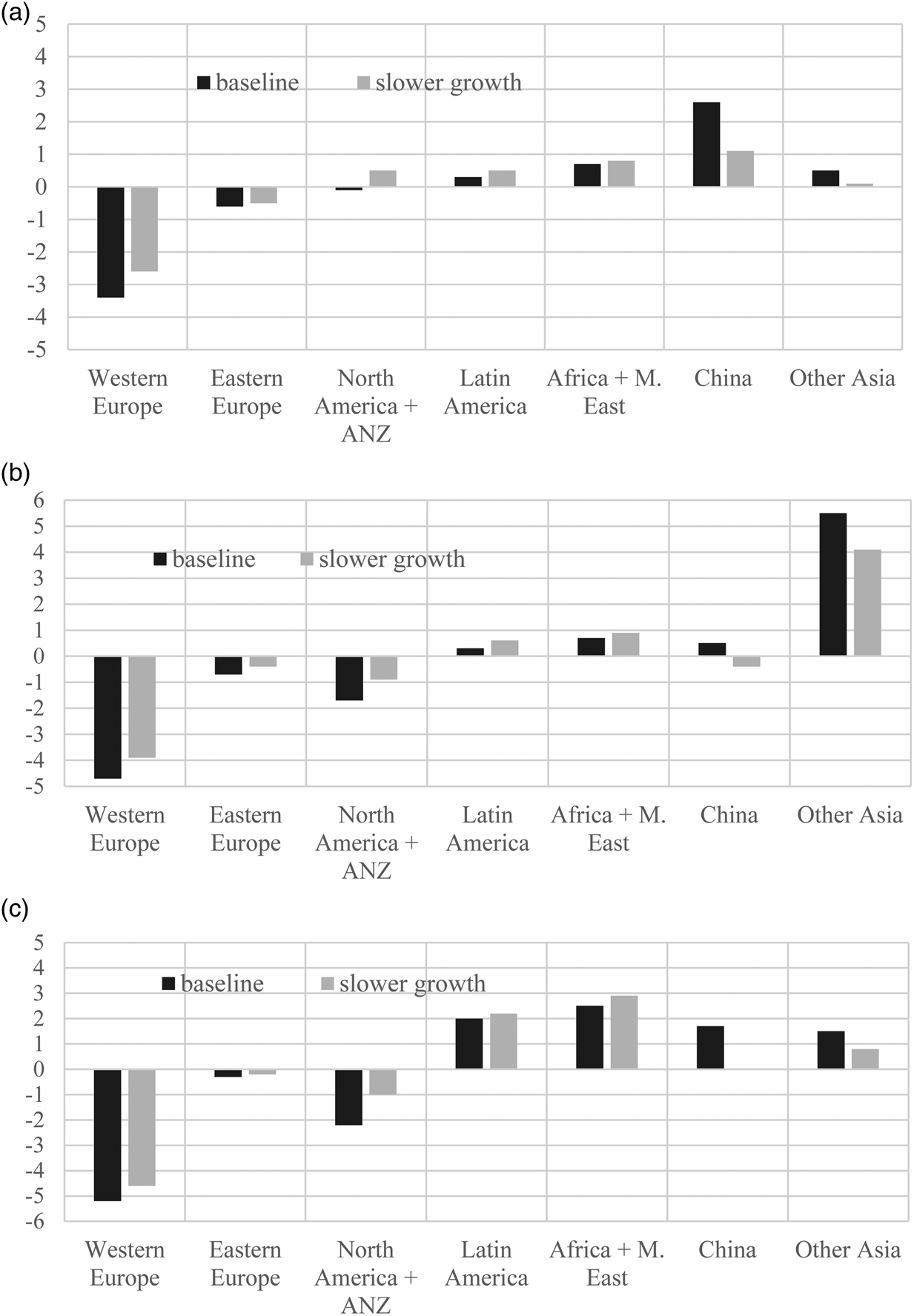
Given the uncertainty associated with economic growth in developing Asia, we also explore here an alternative, slower-growth scenario to the business-as-usual baseline projection to 2025. It assumes Asia's aggregate household incomes grow only two-thirds as fast as in the baseline rates.

The effect this has on projected changes in the shares of the global value of imports of alcohol is shown in Figure 2. Again China stands out, with its domestic wine production continuing to grow slower than its wine consumption. In the business-as-usual scenario, its share of global wine import value rises by 2.6 percentage points between 2016–2018 and 2025, and the rest of Asia's rises by 0.5 percentage points. Africa is the only other region projected to enjoy substantial growth in its share of world wine imports, while Europe is the region whose share is projected to fall by around 3.4 percentage points for Western Europe and 0.6 percentage points for Eastern Europe. But in the slower-growth scenario in which Asia's economies grow only two-thirds as fast over this period, China's share of global wine imports would rise less than half as much (Figure 2, Panel (a)).

Figure 2

Projected Changes in Regional Shares of the Real Value of Global Wine, Spirits, and Beer Imports, 2016–2018 to 2025 (percentage points)

Source: Authors' model projections, business-as-usual and slower Asian growth.

The projected changes in the shares of the global value of imports of spirits and beer are shown in Figure 2 Panels (b) and (c). The overall patterns are similar to that for wine. However, China's growth in importance in global imports increases less for spirits and beer than it does for wine—despite our conservative growth in wine consumption in China over the projection period. In the case of spirits, it is South Asia that dominates projected import growth.

Were we to have assumed a larger preference swing towards wine relative to beer and spirits consumption in China, that country's importance in global wine imports would have been even higher than that shown in Figure 2 Panel (a). That would not have been unreasonable, given that in the above projections, shares of alcohol consumption in China alter very little from 4% for wine, 41% for beer, and 55% for spirits.

We turn now to two variations on the business-as-usual projection, one showing how Brexit might change global beverage markets by 2025, the other showing the effects on those markets of the extra 25% tariff on U.S. imports of some EU beverages that President Trump imposed in late 2019.

V. Effects of Brexit by 2025

The planned withdrawal of the United Kingdom from the EU is non-trivial for the world's beverage markets because the United Kingdom accounts for nearly 11% of the world's wine imports, nearly 4% of global spirits imports, and 25% of global spirits exports in value terms, with half of UK wine imports and two-thirds of UK spirits imports coming from other member countries of the EU. As well, around one-third of UK spirits exports go to other EU member countries.

Brexit has already had a non-trivial impact on markets as the pound has declined by more than 10% against all pertinent currencies since the referendum in June 2016, and UK income and household consumption growth have slowed. Moreover, uncertainty over how the United Kingdom will exit the EU has reduced business investment in the United Kingdom, other EU countries, and non-EU trading partners (Bloom et al., Reference Bloom, Bunn, Chen, Mizen, Smietanka and Thwaites2019; Hassan et al., Reference Hassan, Hollander, van Lent and Tahoun2019). The combined effect of these forces already has reduced the UK's demand for imports of most goods, including beverages, compared with what they would have been had the 2016 referendum voted for the United Kingdom to remain in the EU (Dhingra et al., Reference Dhingra, Huang, Ottaviano, Pessoa, Sampson and Van Reenen2017; Sampson, Reference Sampson2017).

Further effects on beverage markets in the United Kingdom and elsewhere will depend on how the United Kingdom manages its reforms post-Brexit and whether it achieves a “hard” or “soft” exit from the EU. The UK government expects to orchestrate trade deals with numerous non-EU trading partners in addition to the EU in the early part of the current decade, further altering import tariffs and hence bilateral trade flows.

A recent study using the global wine markets model provides projections of the effects of both a “hard” and a “soft” Brexit on global wine markets by 2025 (Anderson and Wittwer, Reference Anderson and Wittwer2018). These effects depend not only on assumed changes in the UK's currency and incomes but also on changes in various bilateral tariffs. The study's “soft Brexit” scenario assumes the United Kingdom will negotiate a free trade agreement (FTA) with the remaining 27 EU member countries and then seek bilateral FTAs with others, including wine-exporting Australia, New Zealand, Chile, and South Africa. Such trade agreements would reduce the loss to wine exporters across the globe compared with a “hard” Brexit involving no such follow-on FTA with the EU, but not by enough to offset the adverse effects of the depreciation of the UK's pound and lowered UK incomes.

Here we re-examine the “soft” Brexit scenario using our new model involving all alcoholic beverages. In this scenario the rate of UK real GDP growth is assumed to be only two-thirds as fast over the projection period 2017–2025 (1.8% per year instead of 2.6%), and the UK pound is assumed to be 10% lower in real terms, than in the model's core baseline “business-as-usual” projection to 2025. It is further assumed the United Kingdom applies the EU's external tariffs on beverages imported from non-EU countries at the end of the agreed transition period but, because of an assumed new bilateral FTA, trade between the UK and EU27 remains duty-free.

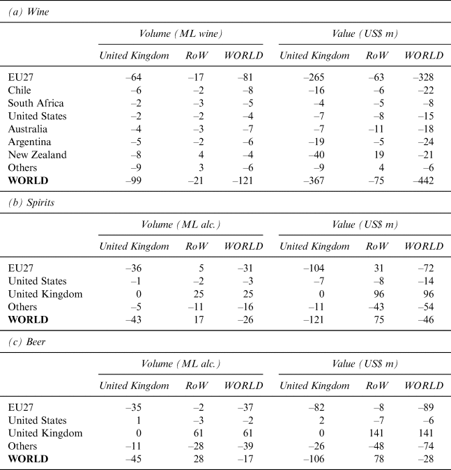
Table 2 suggests that, because of Brexit, the United Kingdom in 2025 would import less beverages from virtually all regions of the world including the EU27, thanks to the United Kingdom being less affluent in the first years following Brexit—and despite an FTA with the EU27 in place of the United Kingdom being in the EU's Single Market. The United Kingdom exports more spirits and beer thanks to declining domestic demand and devaluation of the pound. However, other countries export less beverages because, since their export prices are now lowered, local sales expand. Their export decline is only partly offset by the UK's export expansion, so global beverage trade declines.

Table 2

Difference in 2025 Bilateral Wine and Spirits Import Volumes and Values from Key Exporters by the United Kingdom and Rest of the World (RoW) as a Result of a “Soft” Brexit Shock (ML and 2014 US$ million)

Source: Authors' model results.

VI. Effects of an Extra 25% Tariff on U.S. Imports of Some EU Beverages by 2025

In October 2019, the World Trade Organization published rulings on a long-running dispute between the United States and the EU over subsidies to aircraft manufacturing. The rulings allow the United States to impose tariffs on annual imports of EU products worth up to US$7.5 billion. The finding prompted the United States to impose tariffs on a wide range of EU goods (USTR, Reference USTR2019). They include an additional 25% tariff on still bottled wines with no more than 14% alcohol from France, Germany, Spain, and the United Kingdom, and on Scottish and Irish whiskeys, the aim being to hurt countries that have enjoyed the benefits of EU subsidies to Airbus. Italy and other wine exporters not benefiting from those subsidies were exempted from those new U.S. tariff measures. Champagne and other sparkling wines, high-alcohol (e.g., fortified) wines, and bulk wines in containers greater than two liters, also were exempted, even from the targeted countries.

Such very specific targeting of products that have close substitutes within the beverage group in the targeted countries, and from similar products of other countries, is bound to lead to trade diversion within and across countries. It benefits some firms while hurting others. Some may be able to legally re-label their wines as having, say, 14.5% alcohol, and thereby avoid the extra tariff. Other firms that import bulk wine from targeted countries and bottle it on arrival in the United States will benefit at the expense of competing bottles that continue to be imported directly from those countries. Some U.S. importers or retailers absorbed the tariff hike during the holiday season but started raising prices from January 2020.

Thus U.S. consumers will face higher beverage prices on average while these additional 25% tariffs are in place, and so will lower the quantity they buy. Exporters in the targeted countries not only will sell smaller volumes but also will receive lower prices for targeted products, so the value of their exports will fall more than their volume.

But will this boost exports of other countries, and of substitute products of targeted countries? The answer depends on whether the dampening effect of this extra set of taxes on global alcohol consumption more or less than offsets the positive effects through trade diversion on the consumption of non-targeted products and countries. Those effects, in turn, depend on national shares of U.S. wine imports and U.S. shares of national wine exports. These targeted countries in 2017 accounted for two-fifths of the value of U.S. wine imports, and the United States accounted for 16% of global wine imports.

Furthermore, since these new tariffs are percentage rather than volumetric ($/liter) taxes, they raise the price of affected imported products by more the higher their pre-tax selling price. Hence the share of fine wines in a country's total still bottled wines also matters. The stronger impact on premium wines means prices of grapes are impacted more in countries exporting mainly high-priced wines. It also means some U.S. consumers shift not just to wines at the lower end of the price range and/or to other beverages, but also to fine wines from non-targeted countries.

Our empirical model of global alcohol markets is able to estimate these potentially diverse effects, especially as it is able to distinguish still wines by quality/price/container size and to separate out sparkling wines. We use it here to estimate the producer price, consumer volume, and international trade consequences of these new U.S. tariffs on beverages, focusing on wine because the effects on beer and spirits in this case are much smaller.

A. Producer Price and Consumer Volume Effects

The addition of those selected 25% tariffs is estimated to raise U.S. prices of winegrapes by an average of 2.6%, and producer prices of bottled still wines by 1.1%. Volumes of alcohol consumed in the United States therefore drop, the largest fall being by 1.0% for bottled still wine.

In the targeted countries of France, Germany, and Spain (the United Kingdom is only a tiny exporter of wine and mostly sparkling), average national winegrape prices are estimated to fall by between 1.3% and 2.3%, and producer prices of bottled still wines by between 1.3% and 2.1%. Because of the fall in winegrape prices, non-premium and sparkling wine prices also fall in these countries (by up to 0.2%). The volume of domestic consumption of bottled still wines also, therefore, falls in these countries, by between 0.3% and 0.7%, in the case of super-premium still wines.

In untargeted Italy, by contrast, winegrape prices rise by 1.1%. That helps to raise producer prices of their bottled still wine by 0.7% and to lower their domestic consumption by 0.2%.

Among the New World countries, the estimated impacts differ according to the importance of the U.S. market to their exports and the quality of the wines they sell in that now-more-protected market. Australia's average grape price rises by 0.3%, but New Zealand's rises by 1.4%, and the producer price of bottled still wine rises by 0.2% in Australia and 0.8% in New Zealand. The reason for the larger price rises in New Zealand than in Australia is because New Zealand's exports to the United States account for 33% of New Zealand's total bottled exports compared with only 19% for Australia's exports. Also, New Zealand's exports to the United States have a higher average unit value than Australia's, and so are a closer substitute for the relatively highly-priced EU wines that are now being hit with higher tariffs.

B. Effects on International Trade

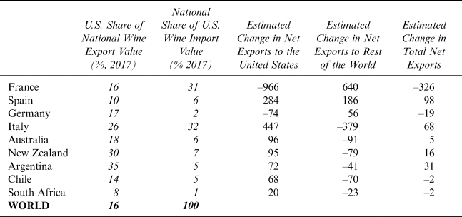
The tariffs reduce world trade in wine by $588 million per year (a fall of 1.6%). Of that total, $491 million is the drop in U.S. wine imports (8.1%). As well, U.S. exports of wine fall by $185 million (11%) as U.S. consumers substitute away from now-dearer imported wines in favor of domestic brands.

Most of the net loss in the global wine trade (more than $300 million) is French fine still wine. Spain has a net export loss of $98 million, while Germany's net export loss amounts to $19 million per year. These targeted countries reduce their exports to the United States by much more than these amounts but expand their exports to other countries, thereby adding to competition elsewhere for countries such as Australia. Untargeted Italy, by contrast, enjoys a net export increase of $68 million, almost all fine wine; and it sells much more to the United States but largely at the expense of sales to other countries (Table 3).

Table 3

Impact of Additional U.S. Wine Import Tariffs of 25% on the Value of Wine Exports Net of Imports, Selected Countries (US$ million per year)

Source: Authors' model results.

Also reported in Table 3 are the impacts of those targeted tariffs on the value of Australian and other New World wine exports net of their imports. As with EU countries, these countries sell much less to the United States, because wines there are now more expensive, so consumption has fallen, and they sell more to the rest of the world.

However, only three of those five New World countries shown in Table 3 enjoy an increase in their total net exports of wine. As foreshadowed above, even non-targeted countries can be worse off from targeted tariffs if those tariffs reduce global consumption sufficiently. In this case, it appears Australian wine exporters are only slightly better off: they sell US$96 million more to the United States and $91 million less to other countries such that their export earnings are raised by just $5 million per year. New Zealand and Argentina enjoy somewhat larger gains, while Chile and South Africa lose slightly. The latter lose because a smaller proportion of their wine exports to the United States are fine wines and so they less-easily displace targeted EU fine wines than do Australian, New Zealand, and Argentinean exports.

VII. Conclusion

The illustrations in the previous sections are just two of many policy scenarios for which the GLOBAL-BEV model is well suited. In addition to trade policy shocks, the model is set up to analyze changes in alcohol consumption taxes. Currently, rates of alcohol taxation, and the types of tax instruments used (e.g., volumetric versus ad valorem), vary enormously between countries. Within each country, they also vary between beverages and often between qualities and styles of each beverage (e.g., sparking versus fortified versus still wines). Health lobbies arguing for increases in alcohol taxes have been successful in some countries (Anderson, Reference Anderson2020a), and that is encouraging similar pressures in other countries. The GLOBAL-BEV model is ideal for simulating such tax changes, especially in the case of countries that are large importers or exporters of beverages because it is able to capture the likely spillovers to other countries' alcohol markets via international trade.

Another use of the GLOBAL-BEV model will be to analyze the likely consequences of the COVID-19 epidemic. That huge shock, and the policy responses of governments to it, is causing a deep recession in many parts of the world economy. Lockdowns and required closures of cafes, restaurants, and bars are hugely reducing on-premise consumption of beverages, but that is being offset to some extent by off-premise (including online) purchases. International trade flows also are being interrupted, and the near-cessation of international tourism is a further blow to demand. These and related consequences could be estimated once the uncertainty around the expected shocks to key exogenous variables dissipates.

Appendix: Structure of the Global Beverage Model

Within the model, wine markets have been disaggregated into four types, namely non-premium (including bulk), commercial-premium, and super-premium still wines, plus sparkling wine. Commercial-premium still wines are defined by Anderson, Nelgen, and Pinilla (Reference Anderson, Nelgen and Pinilla2017) to be those between US$2.50 and $7.50 per liter pre-tax at a country's border or wholesale. Beer and spirits are not split into regular and craft categories, because the latter still have small (albeit growing) market shares in volume terms. The world is divided into 44 individual nations, with all other countries being captured in seven composite residual regions.

A. Production

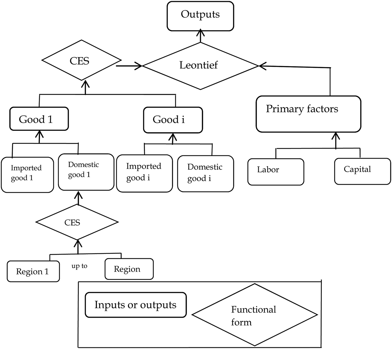
Each industry uses a combination of intermediate and primary inputs to produce a unit of output. Producer decisions consist of a sequence of constant elasticity of substitution (CES) decisions, with a composite good entering the next stage. Figure A1 shows the production structure.

Figure A1

Production Structure of the GLOBAL-BEV Model

Source: Authors' configuration.

Users of commodities minimize costs subject to CES substitutability:

(1)$$X_{ur}^{cs} = f\lpar {X1_{ur}^c \comma \;CES\lsqb {P_{ur}^{cs} /P1_{ur}^c } \rsqb } \rpar $$

(2)$$P1_{ur}^c.X1_{ur}^c = \mathop \Sigma \limits_s X_{ur}^{cs}.P_{ur}^{cs} $$

where $X_{ur}^{cs}$ is the quantity demand of commodity c from (domestic composite or imported) source s by user u (both intermediate and final) in region r. Users include industries, plus a final user, households, in each region. $P_{ur}^{cs}$ is the corresponding price, and $X1_{ur}^c$ and $P1_{ur}^c$ the respective domestic-import composite quantities and prices. Some intermediate inputs such as grapes have endogenous supplies, while others, for whom sales to beverages are a small proportion of total sales, are exogenous implying infinitely elastic supplies.

Throughout the TABLO notation in this section, the index c refers to commodities (COM), s to domestic or imported source (SRC), r to regional destination (REG), u to users (USR), and i to industry (IND ∈ USR).

Next, we outline cost-minimizing behavior in primary factor demands by industry users.

(3)$$L_{ir} = f\lpar {F_{ir}\comma \;CES\lsqb {W_{ir}/PF_{ir}} \rsqb } \rpar $$

(4)$$K_{ir} = f\lpar {F_{ir}\comma \;CES\lpar {R_{ir}/PF_{ir}} \rpar } \rpar $$

(5)$$PF_{ir}.F_{ir} = L_{ir}.W_{ir} + K_{ir}.R_{ir}$$

Equations (3) to (5) show primary factor demands for labor L_ir and capital K_ir, subject to a composite factor demand F_ir by industry i in region r. The factor prices are W_ir for labor, R_ir for capital rentals, and PF_ir for composite prices.

The composite factor demand F_ir is proportional to total output Q_ir subject to a primary-factor using technology A_ir.

(6)$$F_{ir} = Q_{ir}.A_{ir}$$

The demand $X1_{ir}^c$ is related to output Q_ir by a CES relationship between the composite price $P1_{ir}^c$ and the price composite of all intermediate goods P11_ir via a CES function.

(7)$$X1_{ir}^c = f\lpar {Q_{ir}\comma \;CES\lsqb {P1_{ir}^c /P{11}_{ir}} \rsqb } \rpar $$

(8)$$P11_{ir}.X11_{ir} = \mathop \Sigma \limits_c P_{ir}^c.X1_{ir}^c $$

The zero pure profit condition is that total revenue, valued at the output price net of production taxes, PC_ir, multiplied by Q_ir equals the total production cost.

(9)$$PC_{ir}.Q_{ir} = \mathop \Sigma \limits_c P_{ir}^c.X1_{ir}^c + W_{ir}L_{ir} + R_{ir}.K_{ir}$$

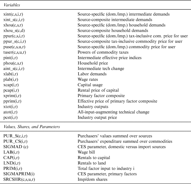
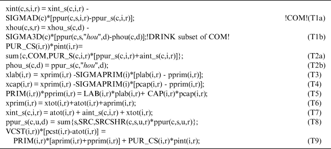
Production variables are defined in Table A1. Listing 1 shows the percentage change quantity equations concerning Equations (1) to (9) in TABLO format.Footnote ¹ The index “hou” refers to the household element of the user set.

Table A1

Definitions of Variables, Values, and Parameters in Production in the GLOBAL-BEV Model

Listing 1.

Production (partial GEMPACK coding) in the GLOBAL-BEV model

B. Commodity Sourcing of Demands

Consumers in a given region source from other regions in common proportions, so that the user subscript is dropped from the equation for CES substitution between import origins:

(10)$$XT_{or}^c = f\lpar {XT1_r^{c\comma "imp"} \comma \;CES\lsqb {PD_{or}^c /PU_r^{c\comma "imp"} \rsqb} } \rpar $$

(11)$$PU_{"imp"\comma r}^c.XT1_r^{c\comma "imp"} = \mathop \Sigma \limits_o XT_{or}^c.PD_{or}^c $$

(12)$$P_{LOCsr}^c = P_{sr}^c.\phi _r/\phi _o$$

(13)$$PD_{or}^c = P_{or}^c.P_{GDP}^o /P_{GDP}^r \quad \quad \quad \quad \quad \lpar {{\rm RawMat}\in {\rm Com}} \rpar $$

(14)$$PD_{or}^c = P_{GDP}^o /P_{GDP}^r.F^{co}\quad \quad \quad \quad \quad \hskip -1pc\lpar {{\rm MatInp}\in {\rm Com}} \rpar $$

(15)$$PD_{or}^c = P_{or}^c + \mathop \Sigma \limits_m P_r^m \quad \quad \quad \quad \quad \lpar {{\rm Drink}\in {\rm Com}} \rpar $$

(16)$$P_r^m = F_r^m.P_{GDP}^r \quad \quad \quad \quad \quad\quad \lpar {{\rm Mar}\in {\rm Com}} \rpar $$

The total demand for all users of commodity c, domestic or import source s, from import origin o to destination d is $XT_{od}^{c\comma "imp"}$. Composite import demands are denoted by $XT_d^{c\comma "imp"}$ and user prices by $PU_d^{c\comma "imp"}$. The delivered price from origin o to destination r is $PD_{or}^c$. GLOBAL-BEV substitutability possibilities involve two stages, between import origins to form the import composite and between the domestic source and import composite.

In the partial equilibrium implementation, there are three subsets within COM. The set MatInp consists of intermediate inputs whose supplies are exogenous. This assumes that changes in beverage input demands have no impacts on the market for these inputs. We need to make judgments as to which food inputs should be endogenous. Grape prices will move with changes in global wine market conditions, as a large share of the global grape crop is crushed to produce wine. Moreover, winegrape varieties differ from table grapes. Grapes are in the RawMat subset of COM. Should grains be exogenous? Barley and wheat used in the manufacture of beverages may account for a significant fraction of local production in some regions, less so nationally. However, we could impose an exogenous shift in supply to depict, for example, a government food policy to divert grains away from beverages towards food production. In a modeling context, this would result in beverage manufacturers switching towards imported grains in response to such a domestic policy.

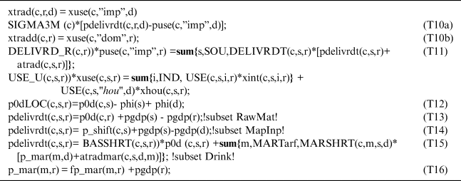
It would be a simple task to allocate various grains to the RawMat subset, but in this implementation of the model, grains are in the MatInp subset of exogenously supplied inputs. Delivered prices for the three subsets of COM (MatInp, RawMat, and Drink) are solved in three distinct groups of equations in GLOBAL-BEV in Equations (13) to (15).

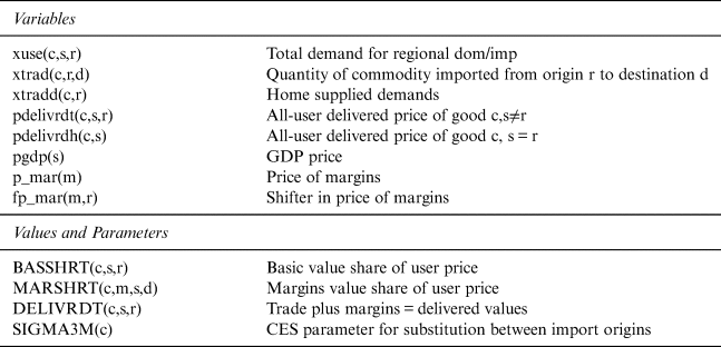
GLOBAL-BEV includes nominal exchange rates relative to the U.S. dollar (the numeraire). Changes in a nation's nominal exchange rate will only affect a producer's competitiveness in global beverage markets if it is transmitted through to real impacts. If a movement in the general price level and in nominal wages exactly offset a nominal exchange rate movement, there is no change in a nation's international competitiveness. We would expect real exchange movements to be reflected in changes in wages and the GDP deflator in a given country relative to the United States, which are exogenous in this partial equilibrium model. The RawMat subset's delivered price is the endogenous basic price $P_{or}^c$ adjusted for GDP deflator movements. The Drink subset delivered price consists of the basic price plus margins. Trade variables are defined in Table A2. Listing 2 outlines the international trade dimension.

Table A2

Definitions of Variables, Values, and Parameters in Trade in the GLOBAL-BEV Model

Listing 2.

International trade (partial GEMPACK coding) in the GLOBAL-BEV model

C. Household Demands

The linear expenditure system (LES) is based on a utility function (U), which splits household spending on each commodity (XHOU_c) into two, a subsistence component XSUB_c that depends only on the number of households (N) and preferences, and a luxury component, XLUX_c that depends on prices and income in a Cobb-Douglas form. β _c is the marginal budget (i.e., aggregate spending minus aggregate subsistence spending) share of commodity c. The regional dimensions are omitted from Equations (17) to (28). The sectors in the household demand system are in the set ComH, which includes the set Drink plus a single sector covering all other household expenditures.

(17)$$U = \displaystyle{1 \over N}\mathop \Pi \limits_c \lpar {XHOU_c-XSUB_c} \rpar ^{\beta _c}$$

Aggregate spending (WHOU) is of the form:

(18)$$WHOU = \mathop \Sigma \limits_c P3_cXHOU_c = \mathop \Sigma \limits_c P3_cXSUB_c + \left[{WHOU-\mathop \Sigma \limits_c P3_cXSUB_c} \right]$$

From this, we obtain the linear expenditure function, where P3_c is the price faced by household consumers of commodity c:

(19)$$P3_cXHOU_c = P3_cXSUB_c + \beta _c\left[{WHOU-\mathop \Sigma \limits_d P3_dXSUB_d} \right]$$

Aggregate subsistence expenditure WSUB is given by:

(20)$$WSUB = \mathop \Sigma \limits_c P3_c.XSUB_c$$

The Frisch “parameter” is the (negative) ratio of total expenditure to luxury expenditure:

(21)$$Frisch = -WHOU/\lsqb {WHOU \ndash WSUB} \rsqb $$

The ORANI school (Dixon et al., Reference Dixon, Parmenter, Sutton and Vincent1982) typically assigns a Frisch “parameter” of –1.82 to a model for a relatively high-income nation.

Differentiating Equation (19) with respect to WHOU, and multiplying by WHOU/[XHOU_c.P3_c], we calculate the expenditure elasticity EPS_c. This is equal to the marginal budget share divided by the budget share (SHOU_c=P3_c.XHOU_c/WHOU) for each commodity:

(22)$$EPS_c = \beta _c.WHOU/\lsqb {P3_c.XHOU_c} \rsqb $$

BLUX_c is the ratio of luxury expenditure to total expenditure on each commodity, given by:

(23)$$BLUX_c = \beta _c\lsqb {WHOU-WSUB} \rsqb /\lsqb {P3_c.XHOU_c} \rsqb $$

Substituting Equations (21) and (22) into Equation (23):

(24)$$BLUX_c = {-}EPS_c/Frisch$$

Next, we calculate the matrix of price elasticities implied by LES. By differentiating Equation (19) with respect to P3_d [i.e., dXHOU _c/dp3_d = −β _cXSUB _d/P3_c], we calculate the off-diagonal elements of the price elasticity matrix (η _cd):

(25)$$\eqalignno{&\hskip 4.7pc dXHOU_c/dP3_d.\lsqb {P3_d/XHOU_c} \rsqb= & (25)\cr & -\beta _c.\lpar {WHOU} \rpar \lpar {P3_dXSUB_d} \rpar /\lpar {WHOU.P3_c} \rpar.\lsqb {P3_d/XHOU_c} \rsqb $$

(26)$$\eta _{cd} = \beta _c\lpar {1-BLUX_d} \rpar.SHOU_d/SHOU_c$$

We obtain the diagonal elements by dividing Equation (22) by P3_c and differentiating with respect to P3_c:

(27)$$\eqalignno{& dXHOU_c/dP3_{c.}\lsqb {P3_c/XHOU_c} \rsqb = {-}\beta _cWHOU/\lsqb {P3_{c.}XHOU_c} \rsqb &(27)\cr & + \Sigma \beta _c\lpar {WHOU} \rpar P3_{d.}XSUB_d/\lsqb {\lpar {WHOU.P3_c} \rpar . \lsqb {P3_{c.}XHOU_c} \rsqb \rsqb} } $$

Substituting Equations (22) and (26) into Equation (27), we obtain:

(28)$$\eta _{cc} = {-}EPS_c-\mathop \Sigma \limits_{d\ne c} \eta _{cd}$$

LES does not allow for specific substitutability. Where appropriate, specific substitutes could form a CES nest, with the CES composite commodity entering LES within the model. In addition, LES does not allow for goods with negative income elasticities.

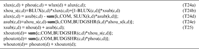
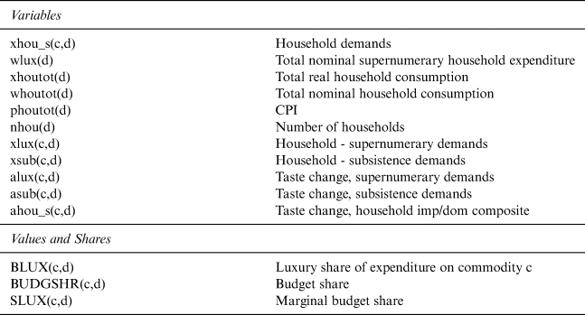
Rather than include the general household demand equation in the model with the elasticities implied by Equations (26) and (28), the LES in GLOBAL-BEV is coded as shown in Listing 3. Definitions of household demand are in Table A3.

Listing 3.

Household demand (partial GEMPACK coding) in the GLOBAL-BEV model

Table A3

Definitions of Variables and Shares in GLOBAL-BEV's Household Demand System

Anderson, Valenzuela, and Wittwer (Reference Anderson, Valenzuela and Wittwer2011) modeled scenarios in which Australia switched from an ad valorem to a volumetric tax on wine. This may induce substitution away from wines with low-unit values towards wines with higher-unit values. The study introduced specific substitution by including a single wine nest in the LES demand system, with CES substitution between different types of wine. The nested wine type would have a single expenditure elasticity.

The CES form is used in two contexts concerning household demand. First, if we wish to have specific substitutability between different beverages, we move the subset of beverages out of the LES form and replace with a CES composite. For example, if fine wine and commercial premium wine are substitutable, a CES composite bottled wine may enter the CES nest:

(29)$$XHOU2_{c1} = f\lpar {XHOU_c\comma \;CES\lsqb {PD_{cl}/P3_c} \rsqb }\rpar $$

In Equation (29), subscript c1 refers to the specific beverages and c the CES composite bottled wine.

The second CES context for households (a subset of users) concerns substitutability by source, in Equation (10).

One simplifying advantage of the partial equilibrium form of GLOBAL-BEV is that additional commodities can be added to the Drink set without altering the existing input-output data. GLOBAL-BEV started with grapes in the RawMat set and wines in the Drink set. In expanding the Drink set, the only modification required to the existing database apart from enlarging the various sales and costs matrices is to subtract the household expenditures of new beverages from the initial sector covering spending on goods and services other than Drink.Footnote ²

D. Margins, Market Clearing, Macro and Tax Collection Equations

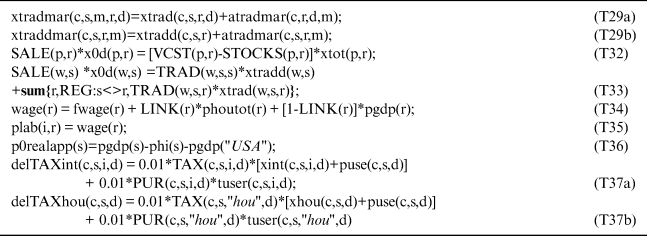
GLOBAL-BEV separates the market for margins from the market for commodities being delivered by margins m (Dixon et al., Reference Dixon, Parmenter, Sutton and Vincent1982). Demands for margins $XTM_{rd}^{csm}$ are proportional to commodity demands $XT_{rd}^{cs}$ subject to a margins-using technology $ATM_{rd}^{csm}$ (Equation (30)).

(30)$$XTM_{rd}^{csm} = ATM_{rd}^{csm}.XT_{rd}^{cs} $$

In Equation (31), $PBAS_r^{cs}$ is the basic commodity price and $PM_{rd}^m$ the margins' prices. $PU_d^{cs}$ is the margins-inclusive, tax-exclusive source-composite delivered price that appears in Equation (15).

(31)$$PD_{rd}^{cs}.XT_{rd}^{cs} = PBAS_r^{cs}.XT_{rd}^{cs} + \sum\limits_m {PM_{rd}^m.XTM_{rd}^{csm}}$$

Equation (32) is the market clearing condition for industry outputs. Additional market clearing equations are required due to the common sourcing assumption. Equation (33) links commodity sales summed across destinations to regional supplies.

(32)$$PTOT_{id}.Q_{id}-XST_{id} = \sum\limits_c {MQ_{cid}} $$

(33)$$\sum\limits_u {X_{ud}^{cs} }.P_{ud}^{cs} = PU_{sd}^c.XT1_d^{cs} $$

Wages (W_r) by region are linked either to the consumer price index (CPI_r) or the GDP deflator ($P_{GDP}^r$) via a binary variable B.

(34)$$W_r = FW_r\lsqb B.P_{GDP}^r + \lpar 1-B\rpar.CPI_r\rsqb $$

(35)$$W_{ir} = W_r$$

The real exchange rate (REXC_r) in each nation relative to the U.S. dollar is given by:

(36)$$REXC_r = P_{GDP}^r /\lsqb P_{GDP}^{"US"}.\phi _r\rsqb $$

Indirect tax collections (TAX_r) from alcohol consumption are a recurring policy issue. $T_{ur}^{cs}$ is the power of the tax by user.

(37)$$TAX_r = \mathop \sum \limits_u \mathop \sum \limits_c \mathop \sum \limits_s PU_{sr}^c.XT1_r^{CS}.\lpar T_{ur}^{CS} -1\rpar $$

A typical scenario in GLOBAL-BEV keeps aggregate consumption in each region exogenous. Since the set Drink accounts for a small share of aggregate consumption, the income effects that might arise from endogenous aggregate consumption are second order.

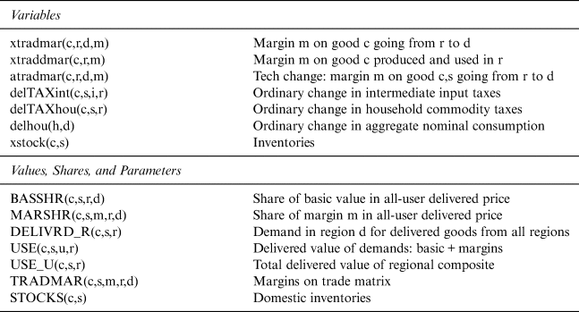
Table A4 contains the definition of variables, values, and shares concerning margins, market clearing, macro and tax collection equations, followed by the TABLO coding in Listing 4.

Table A4

Definitions of Variables, Shares, and Parameters in Margins, Market Clearing, and Tax Collection Equations in the GLOBAL-BEV Model

Listing 4.

Margins (partial GEMPACK coding) in the GLOBAL-BEV model

Footnotes

The authors are grateful for helpful comments from journal referees and financial support from Wine Australia, under Research Project UA1803-3-1, and the University Adelaide's Faculty of the Professions and School of Agriculture, Food & Wine.

¹ Note that the TABLO equation numbering follows that of previous equations in the text: that is, (T7) corresponds with Equation (7).

² The sole exception in this partial equilibrium framework concerns grapes, which are an input of different types of wine plus an input to brandy, which is part of the spirits sector.

References

Anderson, K. (2020a). Consumer taxes on alcohol: An international comparison over time. Journal of Wine Economics, 15(1), 42–70.CrossRef Google Scholar

Anderson, K. (2020b). Asia's emergence in global beverage markets: The rise of wine. Singapore Economic Review, 65(4), 755–779.CrossRef Google Scholar

Anderson, K., Meloni, G., and Swinnen, J. (2018). Global alcohol markets: Evolving consumption patterns, regulations and industrial organizations. Annual Review of Resource Economics, 10(1), 105–32.CrossRef Google Scholar

Anderson, K., Nelgen, S., and Pinilla, V. (2017). Global Wine Markets, 1860 to 2016: A Statistical Compendium. Adelaide: University of Adelaide Press. Available from www.adelaide.edu.au/press/titles/global-wine-markets.CrossRef Google Scholar

Anderson, K., and Pinilla, V. (2020). Annual Database of Global Wine Markets, 1835 to 2018. Wine Economics Research Centre, University of Adelaide. Available from www.adelaide.edu.au/wine-econ/databases.Google Scholar

Anderson, K., Valenzuela, E., and Wittwer, G. (2011). Wine export shocks and wine tax reform in Australia: Regional consequences using an economy-wide approach. Economic Papers, 30(3), 386–399.CrossRef Google Scholar

Anderson, K., and Wittwer, G. (2013). Modeling global wine markets to 2018: Exchange rates, taste changes, and China's import growth. Journal of Wine Economics, 8(2), 132–158.CrossRef Google Scholar

Anderson, K., and Wittwer, G. (2018). Cumulative effects of Brexit and other UK and EU27 bilateral FTAs on the world's wine markets. The World Economy, 41(11), 2883–2894.CrossRef Google Scholar

Bloom, N., Bunn, P., Chen, S., Mizen, P., Smietanka, P., and Thwaites, G. (2019). The impact of Brexit on UK firms. NBER Working Paper 26218, Cambridge, MA, September.CrossRef Google Scholar

Dhingra, S., Huang, H., Ottaviano, G., Pessoa, J. P., Sampson, T., and Van Reenen, J. (2017). The costs and benefits of leaving the EU: Trade effects. Economic Policy, 32(92), 651–705.CrossRef Google Scholar

Dixon, P., Parmenter, B., Sutton, J., and Vincent, D. (1982). ORANI: A Multisectoral Model of the Australian Economy. Contributions to Economic Analysis 142, Amsterdam: North-Holland.Google Scholar

Harrison, J., Horridge, M., Jerie, M., and Pearson, K. (2014). GEMPACK Manual. GEMPACK Software, ISBN 978-1-921654-35-3.Google Scholar

Hassan, T., Hollander, S., van Lent, L., and Tahoun, A. (2019). The global impact of Brexit uncertainty. CEPR Discussion Paper 14253, London, December.Google Scholar

Hertel, T. (ed.) (1997). Global Trade Analysis: Modeling and Applications. Cambridge and New York: Cambridge University Press.Google Scholar

Holmes, A. J., and Anderson, K. (2017). Convergence in national alcohol consumption patterns: New global indicators. Journal of Wine Economics, 12(2), 117–148.Google Scholar

Horridge, M. (2011). The TERM model and its data base. CoPS Working Paper G-219, July. Available from http://ideas.repec.org/p/cop/wpaper/g-219.html.Google Scholar

Sampson, T. (2017). Brexit: The economics of international disintegration. Journal of Economic Perspectives, 31(4), 163–184.CrossRef Google Scholar

United Nations (2019). Comtrade Database. Available from https://comtrade.un.org/db/ (accessed August 15, 2019).Google Scholar

USTR, (2019). Notice of determination and action pursuant to section 301: Enforcement of U.S. WTO rights in large civil aircraft dispute. [Docket No. USTR–2019–0003]. Federal Register, 84(196), 54254–54264.Google Scholar

Wittwer, G., Berger, N., and Anderson, K. (2003). A model of the world's wine markets. Economic Modelling, 20(3), 487–506.CrossRef Google Scholar

Table 1 Cumulative Consumption and Population Growth Rates and Changes in the Real Exchange Rate (RER) Relative to the U.S. Dollar, Business-as-Usual Scenario, 2017 to 2025 (%)

Figure 1 Projected Changes in Regional Shares of the Global Volume of Consumption of Wine, Beer and Spirits, 2016–2018 to 2025 (percentage points)Source: Authors' model projections, business-as-usual.

Figure 2 Projected Changes in Regional Shares of the Real Value of Global Wine, Spirits, and Beer Imports, 2016–2018 to 2025 (percentage points)Source: Authors' model projections, business-as-usual and slower Asian growth.

Table 2 Difference in 2025 Bilateral Wine and Spirits Import Volumes and Values from Key Exporters by the United Kingdom and Rest of the World (RoW) as a Result of a “Soft” Brexit Shock (ML and 2014 US$ million)