1 Introduction
In recent years, in several investigations of supersonic and hypersonic shock wave/boundary layer interactions (SBLI) involving large separated regions, numerical studies have shown multiple vortex structures/eddies embedded in the main separation bubble (Smith & Khorrami Reference Smith and Khorrami1991; Korolev, Gajjar & Ruban Reference Korolev, Gajjar and Ruban2002; Neiland, Sokolov & Shvedchenko Reference Neiland, Sokolov and Shvedchenko2008; Shvedchenko Reference Shvedchenko2009). The critical parameter governing the origin and existence of these eddies seems to be the geometric angle
 $\unicode[STIX]{x1D6FC}^{\ast }=O(Re^{-1/4})$
, which represents the strength of perturbation to the boundary layer such as a shock wave inducing separation at a compression corner or a shock wave from a wedge incident on a boundary layer growing over a surface such as a flat plate beneath the wedge. It must be emphasised that the existence of these eddies is based mainly on numerical simulations of mainly two-dimensional flows involving large separated regions.
In terms of supersonic triple-deck theory, a separation bubble is said to be small when the length of the bubble is
 $O(lRe^{-3/8})$
or less and both separation and reattachment are contained within it. Here,
 $l$
is the characteristic length such as the distance from the leading edge to the compression corner or the point of incidence of an incident shock on a boundary layer over a flat plate;
 $Re$
is a characteristic Reynolds number based on
 $l$
and the free-stream/boundary layer edge conditions. If the bubble length is greater than or equal to
 $O(l)$
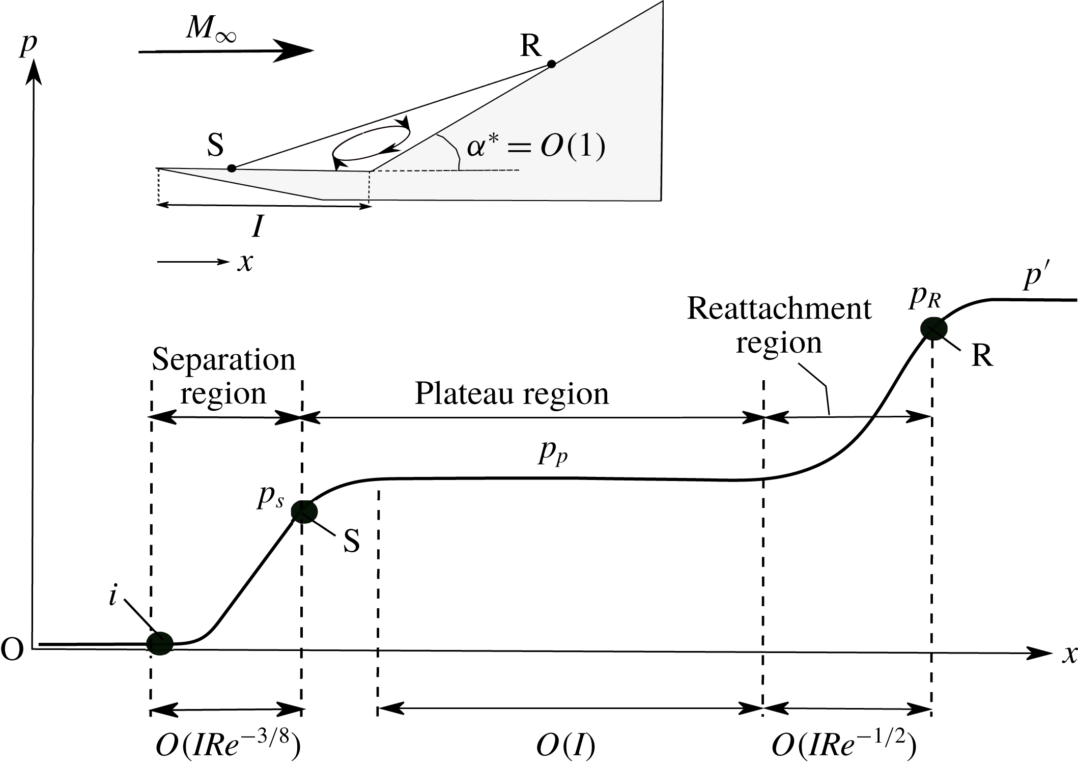
, separation is said to be large, in which case separation and reattachment processes are no longer interconnected but separated by a large region of nearly constant pressure (Burggraf Reference Burggraf1975). Thus, a large separation bubble characteristically consists of three distinct but contiguous regions (figure 1) – an initial rise up to separation, with length
 $O(lRe^{-3/8})$
, a large plateau region of constant pressure
 $O(l)$
, which is followed by the reattachment region of
 $O(lRe^{-1/2})$
in extent that is largely an inviscid process (Burggraf Reference Burggraf1975; Daniels Reference Daniels1979).
With hypersonic flows, there is an additional parameter
 $\unicode[STIX]{x1D70E}$
which includes the effects of both the hypersonic viscous interaction parameter and wall cooling;
 $\unicode[STIX]{x1D70E}$
as defined in Brown, Cheng & Lee (Reference Brown, Cheng and Lee1990) is the ratio of the wall temperature and the critical wall temperature, as in Cheng (Reference Cheng1993).
Typical pressure distribution in a large separated region in a supersonic flow (
 $M_{\infty }<5$
).

Referring to figure 1, the point wherein separation just appears (S), the so-called incipient separation, has a scaled angle
 $\unicode[STIX]{x1D6FC}_{in}=1.57$
where
 $\unicode[STIX]{x1D6FC}$
is defined as in (1.1), and it can be completely described in terms of triple-deck theory. It is also consistent with Chapmans free-interaction theory (Chapman, Kuehn & Larson Reference Chapman, Kuehn and Larson1958). Burggraf (Reference Burggraf1975), Korolev et al. (Reference Korolev, Gajjar and Ruban2002) and Neiland et al. (Reference Neiland, Sokolov and Shvedchenko2008) have shown that large separated regions can be analysed by extending the triple-deck approach.
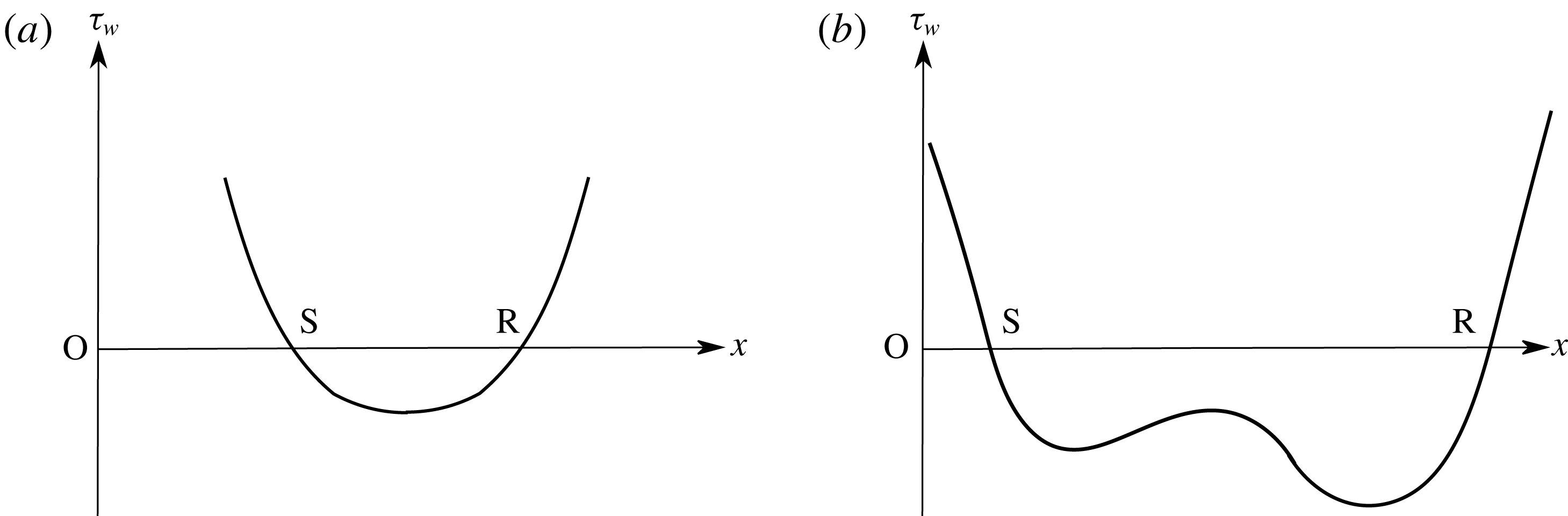
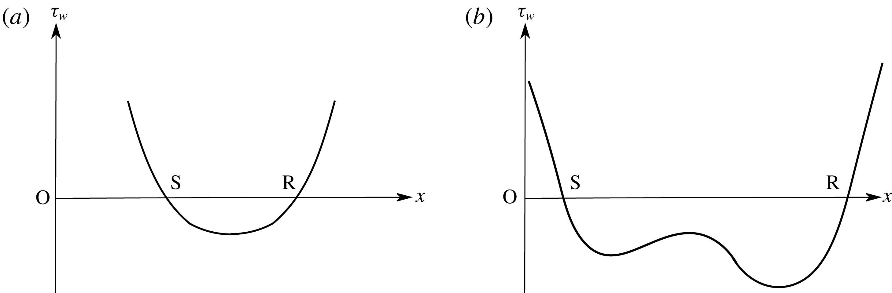
A second characteristic feature of a large separated region is the presence of a second minimum (figure 2) in the shear stress distribution curve immediately before reattachment. It is usually larger and steeper than the first in magnitude. The significance of this second minimum has been discussed previously by Smith (Reference Smith1988), Smith & Khorrami (Reference Smith and Khorrami1991) and Korolev et al. (Reference Korolev, Gajjar and Ruban2002). Its dependence on the scaled angle
 $\unicode[STIX]{x1D6FC}$
has been the subject of much discussion and analysis by Smith (Reference Smith1988), Smith & Khorrami (Reference Smith and Khorrami1991), Korolev et al. (Reference Korolev, Gajjar and Ruban2002) and Neiland et al. (Reference Neiland, Sokolov and Shvedchenko2008).
Shear stress distribution in a small and large separation. (a) Small separation; (b) large separation.
A third characteristic of large separated flows in both supersonic and hypersonic SBLI that has drawn the attention of researchers in recent years is the existence of secondary and even tertiary eddies embedded within the main recirculation region of the separation bubble. Discussion of such a feature in two-dimensional separated flows has been presented by Smith & Khorrami (Reference Smith and Khorrami1991) and Korolev et al. (Reference Korolev, Gajjar and Ruban2002). Further, dependence of such multiple eddies on wall temperature and Reynolds number has recently been investigated by Neiland et al. (Reference Neiland, Sokolov and Shvedchenko2008) and Shvedchenko (Reference Shvedchenko2009), Egorov, Neiland & Shvedchenko (Reference Egorov, Neiland and Shvedchenko2011) and Khraibut et al. (Reference Khraibut, Gai, Brown and Neely2017) in the context of hypersonic SBLI.
In considering large separated regions in supersonic and hypersonic flows, a measure of the extent of separation can be given in terms of the scaled angle
 $\unicode[STIX]{x1D6FC}$
as defined in Stewartson (Reference Stewartson1970)
 $$\begin{eqnarray}\unicode[STIX]{x1D6FC}=\frac{\unicode[STIX]{x1D6FC}^{\ast }Re^{1/4}}{C^{1/4}\unicode[STIX]{x1D706}^{1/2}\unicode[STIX]{x1D6FD}^{1/2}},\end{eqnarray}$$
where
 $\unicode[STIX]{x1D6FC}^{\ast }$
is typically a geometric angle in a compression corner or a corresponding semi-angle of a wedge generating a shock wave incident on a boundary layer developed on a flat plate and provoking separation. Here,
 $Re$
is a characteristic Reynolds number,
 $C$
is the Chapman–Rubesin parameter,
 $\unicode[STIX]{x1D706}$
is a shear constant (0.332 in the case of a Blasius boundary layer) and
 $\unicode[STIX]{x1D6FD}=(M^{2}-1)^{1/2}$
. For hypersonic flows
 $\unicode[STIX]{x1D6FD}\approx M$
.
A comment needs to be made here regarding the definition of the scaled angle
 $\unicode[STIX]{x1D6FC}$
. Different researchers have used different definitions without providing reasons. For example, Neiland et al. (Reference Neiland, Sokolov and Shvedchenko2008) and Shvedchenko (Reference Shvedchenko2009) have used
 $\unicode[STIX]{x1D6FC}=\unicode[STIX]{x1D6FC}^{\ast }Re^{1/4}$
, which ignores the Mach number effect as well as the shear constant and the Chapman–Rubesin parameter of the boundary layer prior to separation. Subsequently, Egorov et al. (Reference Egorov, Neiland and Shvedchenko2011) used
 $\unicode[STIX]{x1D6FC}=\unicode[STIX]{x1D6FC}^{\ast }Re^{1/4}/\unicode[STIX]{x1D6FD}^{1/2}$
, which includes the Mach number but no shear constant and Chapman–Rubesin parameter. Herein, we have used the definition as given in Stewartson (Reference Stewartson1970) and Rizzetta, Burggraf & Jenson (Reference Rizzetta, Burggraf and Jenson1978), which is consistent with the triple-deck assumptions.
Studies by Smith & Khorrami (Reference Smith and Khorrami1991), Korolev et al. (Reference Korolev, Gajjar and Ruban2002) and Shvedchenko (Reference Shvedchenko2009) show that a secondary eddy begins to appear in the recirculating region when
 $4\leqslant \unicode[STIX]{x1D6FC}\leqslant 5$
. A steady secondary eddy persists up to
 $\unicode[STIX]{x1D6FC}\leqslant 6$
. Beyond this, further fragmentation leads to multiple eddies.
Some remarks regarding the existence of secondary eddies in axisymmetric flows may be relevant here. Although substantial computational and experimental effort has been put into investigating double-cone and hollow cylinder/flare hypersonic SBLI (see for example, Holden et al.
Reference Holden, Wadhams, Harvey and Candler2003 and Nompelis, Candler & Holden Reference Nompelis, Candler and Holden2003), involving large separations, there has not been much mention or sufficient discussion of secondary vortices in these flows. Recently, Tumuklu, Levin & Theofilis (Reference Tumuklu, Levin and Theofilis2018) in their discussion of Reynolds number effects on separation over a double-cone flow, have reported the presence of secondary vortex upstream of the junction of the two cones at Reynolds numbers greater than
 $2.8\times 10^{5}$
. The corresponding scaled angle
 $\unicode[STIX]{x1D6FC}$
in this case was 14.3. At a Reynolds number of
 $9.3\times 10^{4}$
, corresponding to
 $\unicode[STIX]{x1D6FC}=11$
, they observed a large separation but no secondary vortex. These values are considerably larger than in the case of a two-dimensional compression corner for steady secondary eddies to exist. Benay et al. (Reference Benay, Chanetz, Mangin, Vandomme and Perraud2006) conducted a numerical and experimental investigation of a hollow cylinder/flare in a Mach 5 flow. The conical flare angle was
 $15^{\circ }$
. The Reynolds number range was
 $3.8\times 10^{5}$
to
 $8.3\times 10^{5}$
when the flow remained laminar. The Reynolds number was based on free-stream conditions and the length
 $L$
, the distance from the leading edge of the cylinder to the cylinder/flare junction. The wall to stagnation temperature ratio was 0.6.
The agreement between experiments and numerical data was good within the laminar range. The authors’ numerical data showed that a secondary eddy, located slightly upstream of the cylinder/flare junction, first appeared at
 $Re_{L}=8.3\times 10^{5}$
with a scaled angle
 $\unicode[STIX]{x1D6FC}=6.1$
. Again, this is higher than the 4–5 predicted by Smith & Khorrami (Reference Smith and Khorrami1991) and Korolev et al. (Reference Korolev, Gajjar and Ruban2002). Benay et al. (Reference Benay, Chanetz, Mangin, Vandomme and Perraud2006) observed multiple eddies at higher Reynolds numbers of
 $16\times 10^{5}$
and
 $22.4\times 10^{5}$
corresponding to
 $\unicode[STIX]{x1D6FC}=7.23$
and 7.86, respectively. They, however, inferred that the secondary eddies are ‘non-physical’ based on their laser Doppler velocimetry (LDV) measurements. They further conjectured that the secondary eddies are a consequence of forcing a two-dimensional laminar Navier–Stokes solution on to an axisymmetric flow and that implementing a three-dimensional solution would result in the formation of Görtler vortices instead, eventually leading to transition.
Gittler & Kluwick (Reference Gittler and Kluwick1987) have analysed laminar separation on an axisymmetric hollow cylinder/flare in an adiabatic wall supersonic flow based on the triple-deck theory. According to these results, large separation (as evidenced by a distinct plateau in the pressure distribution curve) does not occur before
 $\unicode[STIX]{x1D6FC}\approx 9$
. Also, from their shear stress data, it would appear that incipient separation occurs when
 $3\leqslant \unicode[STIX]{x1D6FC}_{in}\leqslant 4$
, which is more than double the two-dimensional incipient separation value of
 $\unicode[STIX]{x1D6FC}_{in}\approx 1.57$
as found by Rizzetta et al. (Reference Rizzetta, Burggraf and Jenson1978). It would, therefore, appear that secondary separation in axisymmetric flow appears at substantially higher values of
 $\unicode[STIX]{x1D6FC}$
compared to the two-dimensional flow.
2 The compression corner geometry
This is a much studied SBLI configuration at supersonic and hypersonic speeds both experimentally (for example, Holden Reference Holden1966; Lewis, Kubota & Lees Reference Lewis, Kubota and Lees1968; Délery & Marvin Reference Délery and Marvin1986; Mallinson, Gai & Mudford Reference Mallinson, Gai and Mudford1997), and numerically (Hung & MacCormack Reference Hung and MacCormack1976; Rudy et al.
Reference Rudy, Thomas, Kumar, Gnoffo and Chakravarthy1989; Olejniczak & Candler Reference Olejniczak and Candler1998; Deepak, Gai & Neely Reference Deepak, Gai and Neely2013). These studies present an exhaustive discussion and analyses of both experimental as well as numerical simulations, which have shown agreement of varying degrees with one another. None of these studies, however, discusses details of the internal structure of the separation bubble such as the presence of secondary vortices and their development mentioned earlier in the Introduction, although some of the above studies did involve large separations. It is only in recent years that existence of secondary vortices in large separated regions induced at a compression corner have been discussed by Neiland et al. (Reference Neiland, Sokolov and Shvedchenko2008) and Shvedchenko (Reference Shvedchenko2009), Egorov et al. (Reference Egorov, Neiland and Shvedchenko2011). These authors have shown that, depending on the magnitude of the scaled angle
 $\unicode[STIX]{x1D6FC}$
, the separated region might develop secondary separation and as a consequence, transverse gradients which ultimately lead to instability, fragmentation and three-dimensional flow.
In the present paper, we have considered one of the experimental flow conditions and the model used in Mallinson (Reference Mallinson1994), and performed an extensive numerical investigation of separated flows ranging from incipient to large separated flows with particular emphasis on the secondary vortices/eddies. The model used was a compression corner consisting of a flat plate 85 mm in length and a ramp plate 95 mm long attached at the end of the flat plate. The ramp plate was adjustable to give a range of corner deflection angles up to
 $24^{\circ }$
. The model span was 180 mm so that the aspect ratio (span/flat plate length) was 2.1. Full geometrical and installation details are given in Mallinson (Reference Mallinson1994).
The flow conditions used in this study are given in table 1, where
 $M,T,p,\unicode[STIX]{x1D70C}$
and
 $Re$
are the Mach number, temperature, pressure, density and Reynolds number, respectively, and subscript
 $\infty$
denotes the free-stream conditions. The flow was laminar throughout and the wall-to-stagnation temperature ratio was 0.125. The value of the hypersonic viscous interaction parameter, based on free-stream and corner conditions, was 1.24. For the present numerical study, six flow deflection angles –
 $10^{\circ }$
,
 $12^{\circ }$
,
 $14^{\circ }$
,
 $16^{\circ }$
,
 $18^{\circ }$
and
 $24^{\circ }$
, were used. These yield near incipient to large separated flows. The scaled angles corresponding to these geometric angles were 2.48, 2.98, 3.47, 3.97, 4.47 and 5.95, respectively.
Mallinson (Reference Mallinson1994) used two more flow conditions in their experiments, apart from that mentioned above. These, however, were lower Reynolds number and Mach number flow conditions. The unit Reynolds numbers were nearly an order of magnitude lower and the Mach number was 7.5. As the main objective of the present investigation concerns the existence of and properties of secondary separation in a large separated flow, and comparison of the results with the asymptotic high Reynolds number theory, the highest Reynolds number and Mach number condition has been used for the present study. This flow condition has been used along with a higher specific enthalpy and lower Reynolds number and Mach number flow condition by Deepak et al. (Reference Deepak, Gai and Neely2013) in another numerical investigation to study the effect of real gas models on separated flows.
Free-stream conditions: condition G in Mallinson (Reference Mallinson1994).

3 Numerical procedure
3.1 Governing equations
In general, the hypersonic SBLI in the continuum flows is accurately described by the compressible Navier–Stokes (N-S) flow equations. The generalised three-dimensional N-S equations for a perfect gas expressed in vector notation are
 $$\begin{eqnarray}\frac{\unicode[STIX]{x2202}\boldsymbol{U}}{\unicode[STIX]{x2202}t}+\frac{\unicode[STIX]{x2202}\boldsymbol{F}}{\unicode[STIX]{x2202}x}+\frac{\unicode[STIX]{x2202}\boldsymbol{G}}{\unicode[STIX]{x2202}y}+\frac{\unicode[STIX]{x2202}\boldsymbol{H}}{\unicode[STIX]{x2202}z}=0,\end{eqnarray}$$
where the vector
 $$\begin{eqnarray}\boldsymbol{U}=\{\unicode[STIX]{x1D70C},\unicode[STIX]{x1D70C}u,\unicode[STIX]{x1D70C}v,\unicode[STIX]{x1D70C}w,E\},\end{eqnarray}$$
where
 $\boldsymbol{F}$
,
 $\boldsymbol{G}$
and
 $\boldsymbol{H}$
are the flux vectors in Cartesian coordinates
 $x$
(streamwise direction),
 $y$
(vertical direction) and
 $z$
(normal to
 $x$
–
 $y$
plane), respectively. In the expression of
 $\boldsymbol{U}$
(equation (3.2)),
 $\unicode[STIX]{x1D70C}$
,
 $T$
,
 $p$
and
 $E$
denote the density, temperature, pressure and total energy per unit volume, respectively. The pressure is calculated using
 $$\begin{eqnarray}p=(\unicode[STIX]{x1D6FE}-1)\unicode[STIX]{x1D70C}\unicode[STIX]{x1D716},\end{eqnarray}$$
where
 $$\begin{eqnarray}\unicode[STIX]{x1D716}=E/\unicode[STIX]{x1D70C}-0.5(u^{2}+v^{2}+w^{2}),\end{eqnarray}$$
and
 $\unicode[STIX]{x1D6FE}$
is the ratio of specific heats
 $c_{p}/c_{v}$
.
 $$\begin{eqnarray}\displaystyle & \displaystyle \boldsymbol{F}=\left[\begin{array}{@{}c@{}}\unicode[STIX]{x1D70C}u\\ \unicode[STIX]{x1D70C}u^{2}+p\\ \unicode[STIX]{x1D70C}vu\\ \unicode[STIX]{x1D70C}wu\\ (E+p)u\end{array}\right]+\left[\begin{array}{@{}c@{}}0\\ \unicode[STIX]{x1D70F}_{xx}\\ \unicode[STIX]{x1D70F}_{yx}\\ \unicode[STIX]{x1D70F}_{zx}\\ \unicode[STIX]{x1D70F}_{xx}u+\unicode[STIX]{x1D70F}_{yx}v+\unicode[STIX]{x1D70F}_{zx}w-k{\displaystyle \frac{\unicode[STIX]{x2202}T}{\unicode[STIX]{x2202}x}}\end{array}\right], & \displaystyle\end{eqnarray}$$
 $$\begin{eqnarray}\displaystyle & \displaystyle \boldsymbol{G}=\left[\begin{array}{@{}c@{}}\unicode[STIX]{x1D70C}v\\ \unicode[STIX]{x1D70C}uv\\ \unicode[STIX]{x1D70C}v^{2}+p\\ \unicode[STIX]{x1D70C}wv\\ (E+p)v\end{array}\right]+\left[\begin{array}{@{}c@{}}0\\ \unicode[STIX]{x1D70F}_{xy}\\ \unicode[STIX]{x1D70F}_{yy}\\ \unicode[STIX]{x1D70F}_{zy}\\ \unicode[STIX]{x1D70F}_{xy}u+\unicode[STIX]{x1D70F}_{yy}v+\unicode[STIX]{x1D70F}_{zy}w-k{\displaystyle \frac{\unicode[STIX]{x2202}T}{\unicode[STIX]{x2202}y}}\end{array}\right], & \displaystyle\end{eqnarray}$$
 $$\begin{eqnarray}\displaystyle & \displaystyle \boldsymbol{H}=\left[\begin{array}{@{}c@{}}\unicode[STIX]{x1D70C}w\\ \unicode[STIX]{x1D70C}uw\\ \unicode[STIX]{x1D70C}vw\\ \unicode[STIX]{x1D70C}w^{2}+p\\ (E+p)w\end{array}\right]+\left[\begin{array}{@{}c@{}}0\\ \unicode[STIX]{x1D70F}_{xy}\\ \unicode[STIX]{x1D70F}_{yy}\\ \unicode[STIX]{x1D70F}_{zy}\\ \unicode[STIX]{x1D70F}_{xz}u+\unicode[STIX]{x1D70F}_{yz}v+\unicode[STIX]{x1D70F}_{zz}w-k{\displaystyle \frac{\unicode[STIX]{x2202}T}{\unicode[STIX]{x2202}z}}\end{array}\right], & \displaystyle\end{eqnarray}$$
and the shear stress tensor is estimated using the Chapman–Enskog approximation as
 $$\begin{eqnarray}\displaystyle & \displaystyle \unicode[STIX]{x1D70F}_{xx}=-\unicode[STIX]{x1D706}\left(\frac{\unicode[STIX]{x2202}u}{\unicode[STIX]{x2202}x}+\frac{\unicode[STIX]{x2202}v}{\unicode[STIX]{x2202}y}+\frac{\unicode[STIX]{x2202}w}{\unicode[STIX]{x2202}z}\right)-2\unicode[STIX]{x1D707}\frac{\unicode[STIX]{x2202}u}{\unicode[STIX]{x2202}x}, & \displaystyle\end{eqnarray}$$
 $$\begin{eqnarray}\displaystyle & \displaystyle \unicode[STIX]{x1D70F}_{yy}=-\unicode[STIX]{x1D706}\left(\frac{\unicode[STIX]{x2202}u}{\unicode[STIX]{x2202}x}+\frac{\unicode[STIX]{x2202}v}{\unicode[STIX]{x2202}y}+\frac{\unicode[STIX]{x2202}w}{\unicode[STIX]{x2202}z}\right)-2\unicode[STIX]{x1D707}\frac{\unicode[STIX]{x2202}v}{\unicode[STIX]{x2202}y}, & \displaystyle\end{eqnarray}$$
 $$\begin{eqnarray}\displaystyle & \displaystyle \unicode[STIX]{x1D70F}_{zz}=-\unicode[STIX]{x1D706}\left(\frac{\unicode[STIX]{x2202}u}{\unicode[STIX]{x2202}x}+\frac{\unicode[STIX]{x2202}v}{\unicode[STIX]{x2202}y}+\frac{\unicode[STIX]{x2202}w}{\unicode[STIX]{x2202}z}\right)-2\unicode[STIX]{x1D707}\frac{\unicode[STIX]{x2202}w}{\unicode[STIX]{x2202}z}, & \displaystyle\end{eqnarray}$$
 $$\begin{eqnarray}\displaystyle & \displaystyle \unicode[STIX]{x1D70F}_{xy}=\unicode[STIX]{x1D70F}_{yx}=-\unicode[STIX]{x1D707}\left(\frac{\unicode[STIX]{x2202}u}{\unicode[STIX]{x2202}x}+\frac{\unicode[STIX]{x2202}v}{\unicode[STIX]{x2202}x}\right), & \displaystyle\end{eqnarray}$$
 $$\begin{eqnarray}\displaystyle & \displaystyle \unicode[STIX]{x1D70F}_{xz}=\unicode[STIX]{x1D70F}_{zx}=-\unicode[STIX]{x1D707}\left(\frac{\unicode[STIX]{x2202}u}{\unicode[STIX]{x2202}z}+\frac{\unicode[STIX]{x2202}x}{\unicode[STIX]{x2202}x}\right), & \displaystyle\end{eqnarray}$$
 $$\begin{eqnarray}\displaystyle & \displaystyle \unicode[STIX]{x1D70F}_{yz}=\unicode[STIX]{x1D70F}_{zy}=-\unicode[STIX]{x1D707}\left(\frac{\unicode[STIX]{x2202}v}{\unicode[STIX]{x2202}z}+\frac{\unicode[STIX]{x2202}w}{\unicode[STIX]{x2202}y}\right). & \displaystyle\end{eqnarray}$$
Here,
 $\unicode[STIX]{x1D707}$
and
 $\unicode[STIX]{x1D706}$
are the first and second coefficients of viscosity, respectively, whereas
 $k$
is the thermal conductivity.
The flux terms (equations (3.5)–(3.7)) can be conveniently decomposed into inviscid and viscous terms such that
 $$\begin{eqnarray}\boldsymbol{A}=\boldsymbol{A}_{i}+\boldsymbol{A}_{v},\end{eqnarray}$$
where
 $A$
is generic for any of the
 $\boldsymbol{F}$
,
 $\boldsymbol{G}$
and
 $\boldsymbol{H}$
vectors and subscripts ‘
 $i$
’ and ‘
 $v$
’ denote inviscid and viscous components, respectively. It should be pointed out that the first rows in (3.5)–(3.7) refer to the conservation mass terms, rows 2–4 are the conservation of momentum terms and row 5 terms are associated with the conservation of energy. The
 $\unicode[STIX]{x1D70F}$
terms in (3.7) and (3.13) moreover assume a homogeneous, isotropic Newtonian fluid and only change with velocity gradients.
3.2 Description of solver, free-stream conditions and simulations
Numerical simulations of a compression corner for various deflection angles were carried out using a continuum flow solver US3D. US3D was developed at the University of Minnesota specifically for high-speed flows (Nompelis & Candler Reference Nompelis and Candler2014; Candler et al. Reference Candler, Johnson, Nompelis, Gidzak, Subbareddy and Barnhardt2015). It is capable of carrying out both perfect gas and real gas simulations, and has been validated for a wide range of hypersonic flow problems (Drayna, Nompelis & Candler Reference Drayna, Nompelis and Candler2006; Candler, Subbareddy & Brock Reference Candler, Subbareddy and Brock2014; MacLean, Holden & Dufrene Reference MacLean, Holden and Dufrene2014). The code uses parallel processing to improve computational speed and allows both implicit and explicit time integrations to be conducted.
Representation of the discretised N-S equations expressed in the implicit formulation as well as the resolution of viscous and inviscid terms to obtain a finite volume representation of the N-S equations have been given in Wright, Candler & Bose (Reference Wright, Candler and Bose1998).
Steady-state solutions in US3D are obtained using the modified Steger–Warming flux vector splitting method (Candler et al. Reference Candler, Johnson, Nompelis, Gidzak, Subbareddy and Barnhardt2015), and the Jacobians are evaluated such that the dissipation is low, as typically required in hypersonic simulations (Wright et al. Reference Wright, Candler and Bose1998; MacCormack Reference MacCormack2014). The solver uses the monotonic upstream-centred (MUSCL) scheme of Van Leer (Reference Van Leer1979) to give second-order spatially accurate solutions. The code permits the use of flux limiters to prevent non-physical solutions from occurring (MacCormack Reference MacCormack2014). The default Osher limiter (Nompelis & Candler Reference Nompelis and Candler2014) is utilised in the present simulations, having good dissipation characteristics.
Data parallel line relaxation (DPLR) which is implemented in US3D is capable of handling stretched cells seen in hypersonic applications, without degrading the method’s performance (Wright et al. Reference Wright, Candler and Bose1998). The DPLR method, however, requires more memory storage compared to other methods, while it is also able to converge at a much faster rate (Wright et al. Reference Wright, Candler and Bose1998). Implicit time integration is chosen in the study to allow large Courant–Friedrichs–Lewy (CFL) numbers to be used.
Two-dimensional simulations assume a laminar flow given the moderate Reynolds number flow under consideration. They also take the walls to be non-catalytic and impose a no-slip boundary condition on the walls. The operating gas is taken as a 5-species air, and the simulations are based on the perfect gas assumption.
The viscosities are evaluated using Blottner curve fits and Wilke’s mixing rule for the mixture (Wilke Reference Wilke1950; Blottner, Johnson & Ellis Reference Blottner, Johnson and Ellis1971), while thermal conductivities are calculated using Eucken’s correction (Candler et al. Reference Candler, Johnson, Nompelis, Gidzak, Subbareddy and Barnhardt2015).
The free-stream conditions used for this compression corner study described in § 2 are based on experimental condition G in Mallinson (Reference Mallinson1994), Mallinson et al. (Reference Mallinson, Gai and Mudford1997), Olejniczak & Candler (Reference Olejniczak and Candler1998) and Deepak et al. (Reference Deepak, Gai and Neely2013). Separate grid independence studies were carried out for these flow conditions by Olejniczak & Candler (Reference Olejniczak and Candler1998) and Deepak et al. (Reference Deepak, Gai and Neely2013) for corner angles
 $\unicode[STIX]{x1D6FC}^{\ast }=10^{\circ }$
and
 $18^{\circ }$
. For
 $\unicode[STIX]{x1D6FC}^{\ast }=18^{\circ }$
, Olejniczak & Candler (Reference Olejniczak and Candler1998) indicated grid independence with
 $262\times 10^{3}$
cells. Deepak et al. (Reference Deepak, Gai and Neely2013), on the other hand, used a much coarser grid with
 $60\times 10^{3}$
cells, using the time accurate code Eilmer3 of Jacobs & Gollan (Reference Jacobs and Gollan2010).
In the present study, we consider compression angles starting from incipient separation at
 $10^{\circ }{-}18^{\circ }$
with 2 degree increments, and finally
 $24^{\circ }$
, which yields a large separation. The grid independence study was carried out for the
 $18^{\circ }$
deflection angle because it yields a sufficiently large separation, and is also sufficient to verify the other cases. The finest grid for this case is therefore used in the simulations of other deflection angles.
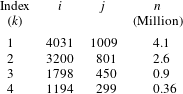
Table 2 summarises the grids used in the grid independence study, where cell numbers varied between nearly 360 000 cells in the coarsest grid and 4 million cells in the finest. Index
 $k$
in the table refers to the grids in a descending order,
 $i$
being the number of nodes in the streamwise direction and
 $j$
the number of nodes in the transverse direction, with
 $n$
is the total number of cells.
Summary of grids used in grid convergence study (
 $\unicode[STIX]{x1D6FC}^{\ast }=18^{\circ }$
).

3.3 Convergence study
Surface data, shear stress, pressure and heat flux are monitored to determine convergence of the solution. This convergence study considers the
 $18^{\circ }$
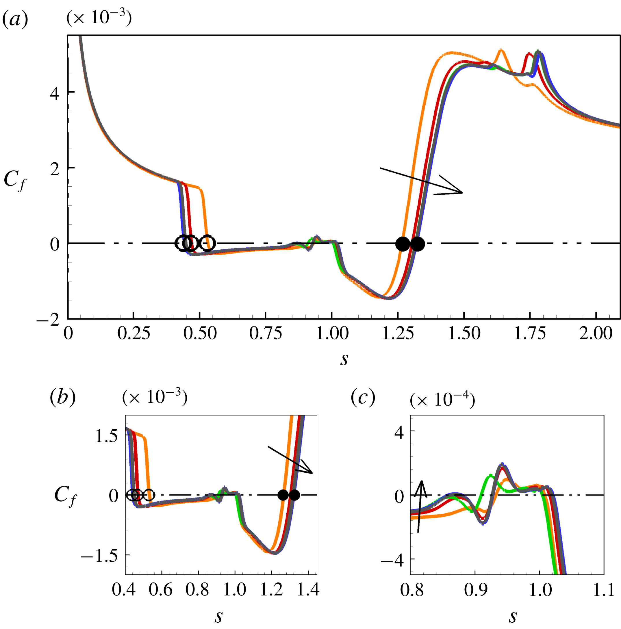
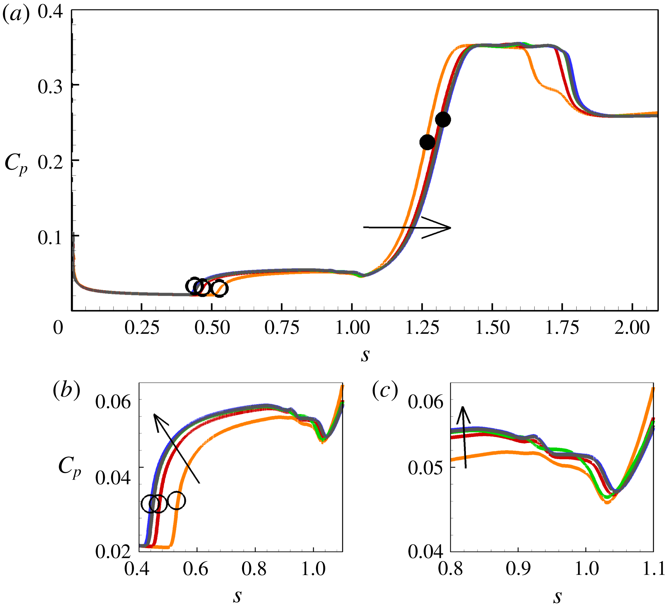
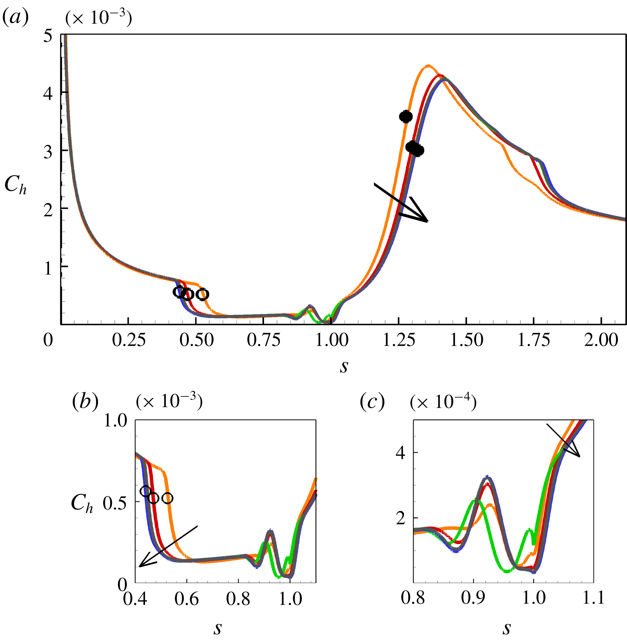
compression angle, which yields a sufficiently large separated region and can be validated against the experimental data of Mallinson (Reference Mallinson1994). The shear stress is important because it defines the length of separation as it crosses the zero line from positive to negative at separation and negative to positive at reattachment. The pressure and heat flux, on the other hand, are experimentally measurable quantities in short-duration facilities. The surface parameters are shown on a global scale for grids 1–4 in figures 3–5, where
 $s$
is the non-dimensional wetted distance
 $s^{\ast }/L$
where
 $L$
is the length of the flat plate,
 $C_{f}$
is the ratio of wall shear stress to dynamic pressure
 $0.5\unicode[STIX]{x1D70C}_{\infty }\boldsymbol{U}_{\infty }^{2}$
,
 $C_{p}$
is the surface pressure to dynamic pressure ratio and
 $C_{h}$
is the heat flux to the quantity
 $0.5\unicode[STIX]{x1D70C}_{\infty }\boldsymbol{U}_{\infty }^{3}$
ratio. It was also noted that all grids reached steady state with a minimum of a five order drop in root mean square (RMS) residuals, and in these figures, the different curves pertain to these steady-state solutions for each grid.
Considering figure 3, which shows the shear stress data, the size of the recirculation region is determined as the shear stress crosses the zero line from positive to negative at separation and from negative to positive at reattachment (see (a) and (b)). Multiple crossings of the zero line indicate fragmented vortices within the main separation region ((b) and (c)). During the grid independence study, it was noted that these secondary structures within the primary separation are quite sensitive to first cell height and level of convergence of the solution, and the attainment of a steady state.
Pressure and heat flux data are similarly shown in figures 4 and 5 with the magnified views of the corner flow shown in (b) and (c) of the figures. We also note changes of pressure and heat flux with grid refinement. It should be noted also that grid 4 used in the present simulations is of the same size as the reported converged grid in Deepak et al. (Reference Deepak, Gai and Neely2013) using a time explicit solver (
 ${\approx}360~\text{K}$
cells). The present simulations show that at least ten times the number of cells in that grid compared to grid 2 (at least 3 millions) were required to reach convergence.
Convergence of the shear stress
 $C_{f}$
in the
 $\unicode[STIX]{x1D6FC}^{\ast }=18^{\circ }$
compression corner case. Blue: grid 1; green: grid 2; red: grid 3; orange: grid 4. Open circles: separation; closed circles: reattachment. Arrow points in direction of increased grid refinement. (a) Global distribution; (b) main separation; (c) near the vertex.

Convergence of the surface pressure
 $C_{p}$
in the
 $\unicode[STIX]{x1D6FC}^{\ast }=18^{\circ }$
compression corner case. Blue: grid 1; green: grid 2; red: grid 3; orange: grid 4. Open circles: separation; closed circles: reattachment. Arrow points in direction of increased grid refinement. (a) Global distribution; (b) main separation; (c) near the vertex.

Convergence of the heat flux
 $C_{h}$
in the
 $\unicode[STIX]{x1D6FC}^{\ast }=18^{\circ }$
compression corner case. Blue: grid 1; green: grid 2; red: grid 3; orange: grid 4. Open circles: separation; closed circles: reattachment. Arrow points in direction of increased grid refinement. (a) Global distribution; (b) main separation; (c) near the vertex.

Separation length
 $l_{B}$
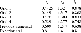
is a good measure of the quality of the numerical solution as pointed out by Druguet, Candler & Nompelis (Reference Druguet, Candler and Nompelis2005). Table 3 compares the non-dimensional locations of separation (
 $s_{S}$
) and reattachment
 $s_{R}$
, and the separation length
 $l_{B}$
in the present grid convergence study for all four grids and those for the reported converged grid by Deepak et al. (Reference Deepak, Gai and Neely2013). It is seen that the present simulations show an increase of 27.3 % in the separation length
 $l_{B}$
, occurring mainly as a result of separation point moving upstream by 37.62 %, and reattachment moving downstream by 5.52 %. The experimental data from Mallinson (Reference Mallinson1994) indicate that the non-dimensional length of separation for condition G at
 $\unicode[STIX]{x1D6FC}^{\ast }=18^{\circ }$
is 0.8. The computations, therefore, seem to over-predict the same length by less than 10 %.
Comparison of separation length with previous numerical study of Deepak et al. (Reference Deepak, Gai and Neely2013) and experiments of Mallinson (Reference Mallinson1994) for a compression angle of
 $\unicode[STIX]{x1D6FC}^{\ast }=18^{\circ }$
.

3.4 Grid error analysis
The mixed-order method is used to carry out a systematic grid error analysis as it deals well with flow discontinuities such as shock waves. The method has been described in detail by Roy (Reference Roy2003) by retaining both first-order and second-order terms in the generalised Richardson extrapolation technique
 $$\begin{eqnarray}f=f_{exact}+g_{1}h+g_{2}h^{2}+O(h^{3}),\end{eqnarray}$$
which requires all grid solutions to be within the asymptotic range of
 $f_{exact}$
and continuous. Expanding (3.15) to at least three grids yields an exact solution as
 $$\begin{eqnarray}f_{exact}=f_{1}+\frac{\unicode[STIX]{x1D716}_{32}(r_{12}-1)-\unicode[STIX]{x1D716}_{21}(r_{12}r_{23}^{2}-r_{12}-r_{23}-1)}{(r_{12}-1)(r_{23}-1)(r_{12}r_{23}-1)},\end{eqnarray}$$
where
 $\unicode[STIX]{x1D716}_{32}=f_{3}-f_{2}$
,
 $\unicode[STIX]{x1D716}_{21}=f_{2}-f_{1}$
,
 $r_{12}=h_{1}/h_{2}$
,
 $r_{23}=h_{2}/h_{3}$
.
Here,
 $f_{exact}$
can be evaluated for any parameter of interest to convergence, which in the case of separated flows are the surface parameter at separation
 $S$
and reattachment
 $R$
as
 $$\begin{eqnarray}|\text{Spatial error}|=3\left|\frac{f_{1-3}-f_{exact}}{f_{exact}}\right|\times 100,\end{eqnarray}$$
where the number three seen in the equation is a safety factor to give a conservative estimate of the error.
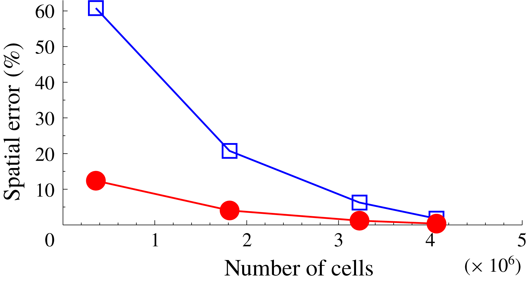
Figure 6 shows changes of the spatial error with grid refinement in terms of the number of cells used in each grid. The blue square symbols denote the location of separation, while the closed red circles denote reattachment. In the figure, the coarsest grid 4 yielded the highest error values at separation (
 ${\approx}60\,\%$
) and reattachment (
 ${\approx}10\,\%$
). This shows that the location of separation
 $s_{S}$
is more sensitive to grid refinement that the location of reattachment
 $s_{R}$
. It can be noted further that grid 2 yields spatial error values within 6 % of the exact locations of separation and reattachment. Discussion of results to follow is based on the finest grid 1 solutions which show separation to be within 2 % of the exact value with a safety factor of three. This grid size is therefore used for other compression angles.
Changes in spatial error with grid refinement in terms of the number of cells. Blue squares: separation; red circles: reattachment.

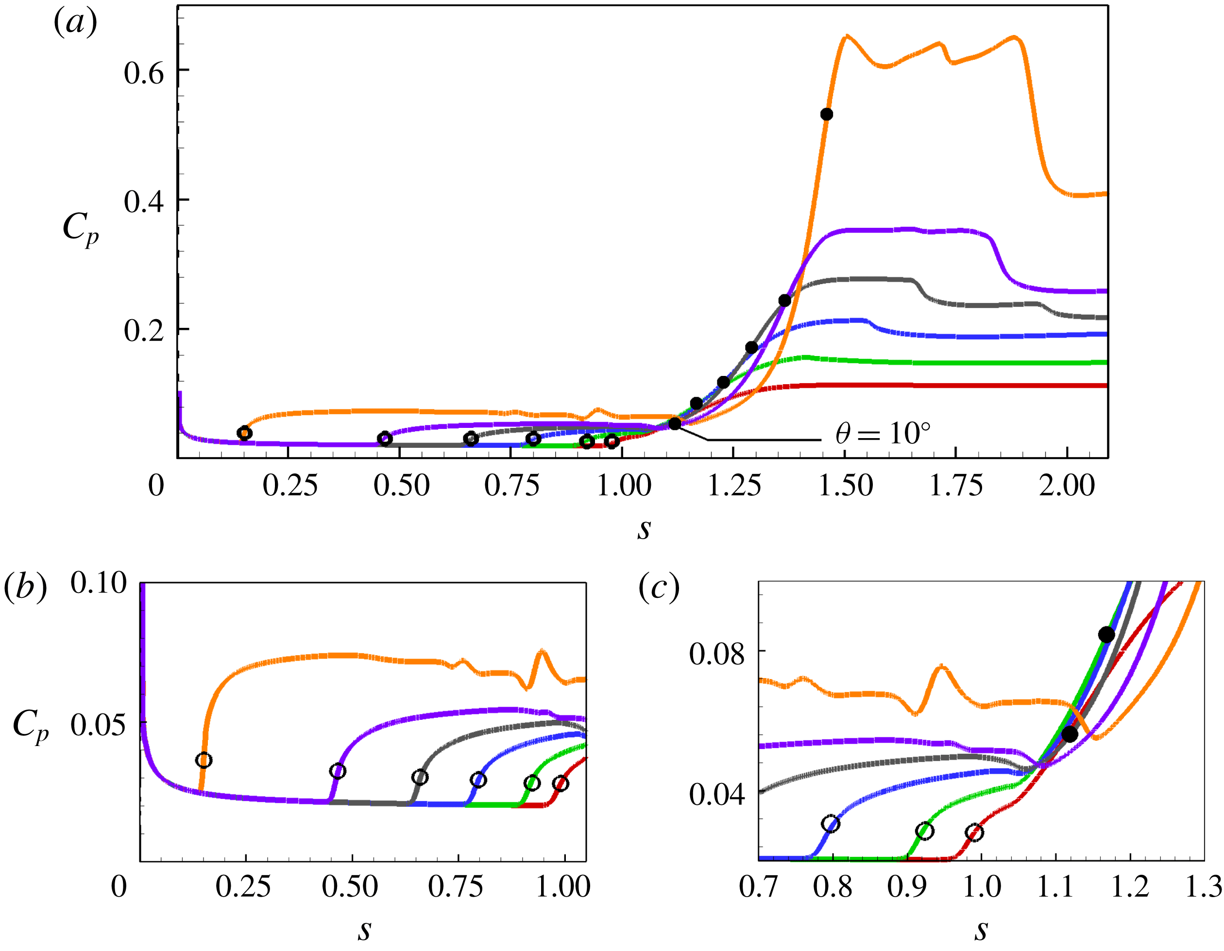
Variation of pressure with different deflection angles. Red:
 $10^{\circ }$
; green:
 $12^{\circ }$
; blue:
 $14^{\circ }$
; grey:
 $16^{\circ }$
; purple:
 $18^{\circ }$
; orange:
 $24^{\circ }$
. Open circles: separation; closed circles: reattachment. (a) Global distribution; (b) near the leading edge; (c) near the corner.

4 Results and discussion
4.1 General flow characteristics
Figures 7 and 8 show results for non-dimensional surface pressure
 $C_{p}$
and shear stress
 $C_{f}$
, respectively, for these deflection angles.
The pressure curves (figure 7) illustrate all the major features of moderate to large separated regions as delineated in figure 1. The initial rise in pressure up to separation (open circles) is followed by a distinct plateau after approximately
 $12^{\circ }$
, after which it grows with the increase in the corner angle. At the largest corner angle of
 $24^{\circ }$
, we note three distinct peaks after reattachment. These peaks are the result of multiple vortices, as will be shown later. The inset in the figure shows the pressures in the vicinity of the corner. Again, we notice some significant fluctuations with the
 $24^{\circ }$
angle. We also note that as the corner is approached, there is a local drop in pressures, which is indicative of secondary vortices (see Smith & Khorrami Reference Smith and Khorrami1991; Korolev et al.
Reference Korolev, Gajjar and Ruban2002; Egorov et al.
Reference Egorov, Neiland and Shvedchenko2011).
This dip in pressure is particularly noticeable for angles
 $16^{\circ }$
,
 $18^{\circ }$
and
 $24^{\circ }$
, corresponding to scaled angles of 3.97, 4.47 and 5.95, respectively. This is consistent with the previous observations of Smith & Khorrami (Reference Smith and Khorrami1991), Korolev et al. (Reference Korolev, Gajjar and Ruban2002) and Shvedchenko (Reference Shvedchenko2009) that steady secondary separation appears at
 $3\leqslant \unicode[STIX]{x1D6FC}\leqslant 4$
and instability in secondary separation and fragmentation occurs when
 $\unicode[STIX]{x1D6FC}\geqslant 6$
. Another feature to note is that the rise to reattachment and peak pressure becomes steeper with increasing corner angle and so also the fall after reaching the peak.
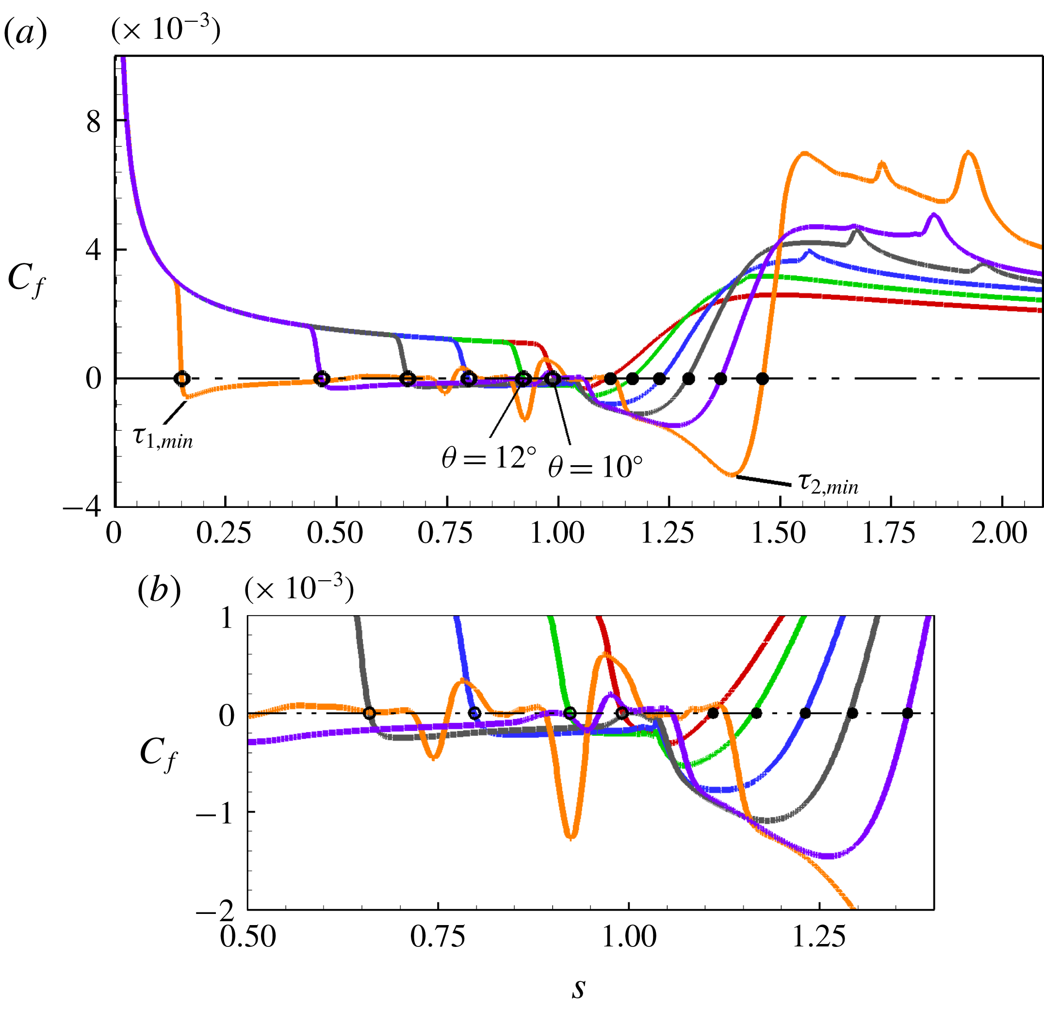
Figure 8 shows the corresponding shear stress curves for these corner angles. They show the large changes occurring within the separated region with increasing deflection angle. After the near incipient separation with the
 $10^{\circ }$
angle, the increase in separation length from
 $12^{\circ }$
to
 $24^{\circ }$
is more than fivefold. In this process, the separation point moves upstream and reattachment moves downstream. Multiple positive peaks with increasing corner angles are indicative of a number of secondary vortices. Another interesting feature is that at higher corner angles of
 $18^{\circ }$
and
 $24^{\circ }$
a ‘knee’ seems to appear on the front leg of the second minimum in shear stress corresponding to
 $\unicode[STIX]{x1D6FC}=4.47$
and
 $\unicode[STIX]{x1D6FC}=5.95$
, respectively. Note also the steep rise in shear stress immediately after reaching the minimum and after reattachment (when the shear stress becomes positive) as the corner angle is increased.
Variation of shear stress with deflection angle. Red:
 $10^{\circ }$
; green:
 $12^{\circ }$
; blue:
 $14^{\circ }$
; grey:
 $16^{\circ }$
; purple:
 $18^{\circ }$
; orange:
 $24^{\circ }$
. Open circles: separation; closed circles: reattachment. (a) Global distribution; (b) near the corner.

Density gradients
 $(\text{Kg}~\text{m}^{-4})$
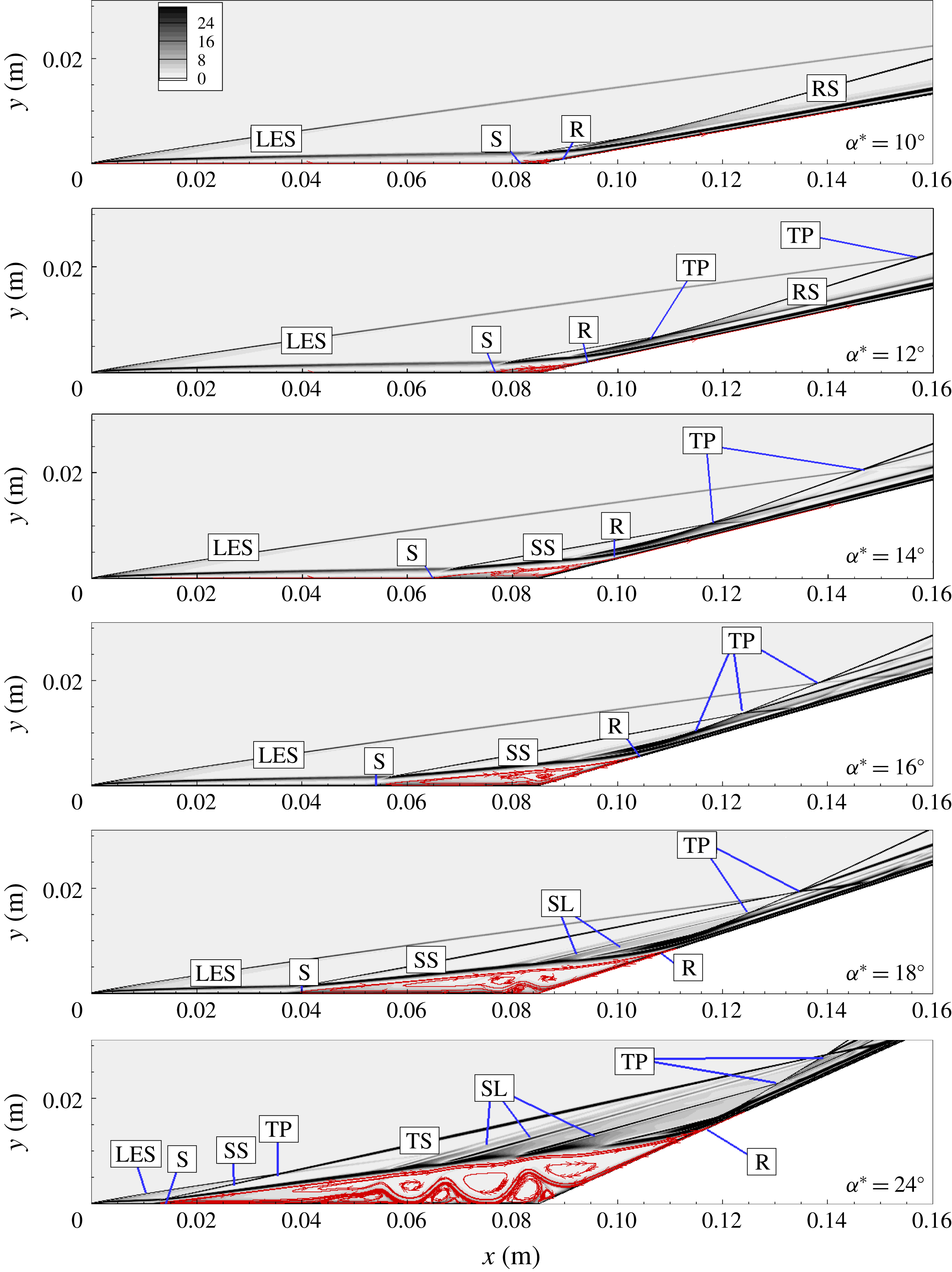
for the different deflection angles with streamlines superposed. LES, leading edge shock; SS, separation shock; TP, triple point; SL, shocklets; RS, recompression shock; TS, transmitted shock; S, separation; R, reattachment; DSL, dividing streamline.

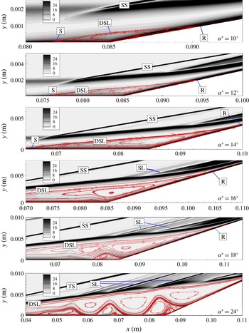
Density gradients
 $(\text{Kg}~\text{m}^{-4})$
for the different deflection angles with streamlines superposed: corner region.

Figures 9 and 10 respectively show global density gradients in the separated regions and in the corner region for all angles. In the figures the streamlines are superposed with major flow features annotated. These figures enable us to identify shock and compression waves at separation and reattachment, as well as vortices in the separated regions. Major features such as the leading edge shock (LES), separation shock (SS), reattachment shock (RS) and the triple point (TP) can all be identified. Secondly, at the
 $10^{\circ }$
angle, we can see that separation (S) is about to develop. This is in agreement with the experimental result of Mallinson (Reference Mallinson1994), who found that the incipient separation angle was
 $10^{\circ }\pm 2^{\circ }$
. Secondary vortices begin to appear at the
 $16^{\circ }$
deflection angle at a corresponding scaled angle of
 $\unicode[STIX]{x1D6FC}=3.97$
. At
 $18^{\circ }$
and
 $24^{\circ }$
corresponding to
 $\unicode[STIX]{x1D6FC}=4.47$
and 5.95, we can identify three and eight vortices respectively within the separated region. Note that in the large deflection angle
 $18^{\circ }$
, the wall vortices (total of three) become fragmented as well. An interesting feature here is that, corresponding to the crest of these embedded vortices, compression waves (SL) seem to originate, which manifest themselves as peaks in the pressure curves seen in figure 7.
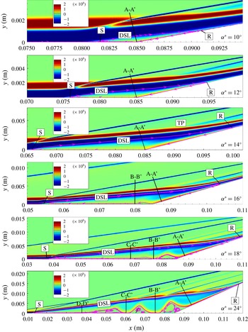
Figure 11 shows the vorticity distribution in the separated regions for all deflection angles. Section A-A’ denotes the wall normal at the corner for angles
 $10^{\circ }{-}14^{\circ }$
and the reverse flow boundary layer as it separates for angles
 $16^{\circ }{-}24^{\circ }$
. We note small distortions (see sections A-A’ to D-D’ fore angles
 $16^{\circ }{-}24^{\circ }$
in the figure) begin to occur at
 $16^{\circ }$
angle corresponding to
 $\unicode[STIX]{x1D6FC}=3.97$
and fragmentation into three secondary vortices has occurred at
 $18^{\circ }$
with
 $\unicode[STIX]{x1D6FC}=4.47$
. At the
 $24^{\circ }$
corner angle with
 $\unicode[STIX]{x1D6FC}=5.95$
further fragmentation into eight secondary vortices has taken place.
Vorticity
 $\unicode[STIX]{x1D714}_{z}$
contours
 $(1~\text{s}^{-1})$
for the different deflection angles with major streamlines superposed. A-A’, wall normal at the reverse flow boundary layer or corner; B-B’ to D-D’, wall normals at each vortex.

These general flow features of large separated flows, namely, two shear stress minima, a distinct pressure plateau and multiple secondary vortices, are consistent with the studies by Smith & Khorrami (Reference Smith and Khorrami1991), Korolev et al. (Reference Korolev, Gajjar and Ruban2002) and Shvedchenko (Reference Shvedchenko2009) (see figures 4
a and 4
b). Our results also agree with Shvedchenko’s observation that steady secondary separation first occurs when
 $3\leqslant \unicode[STIX]{x1D6FC}\leqslant 4$
and considerable fragmentation takes place when
 $\unicode[STIX]{x1D6FC}>4.5$
.
4.2 Shear stress and pressure gradient in the reversed flow region
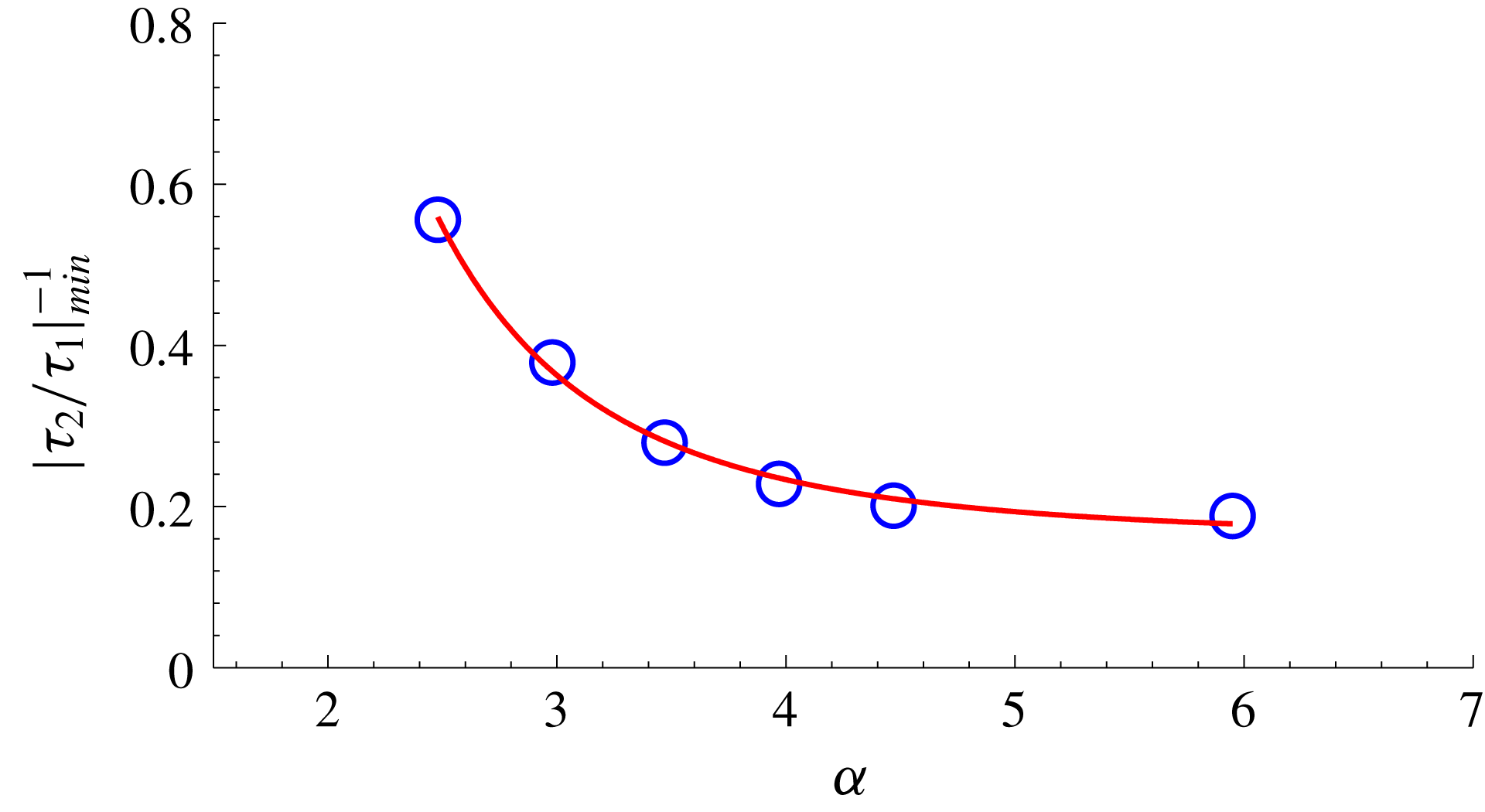
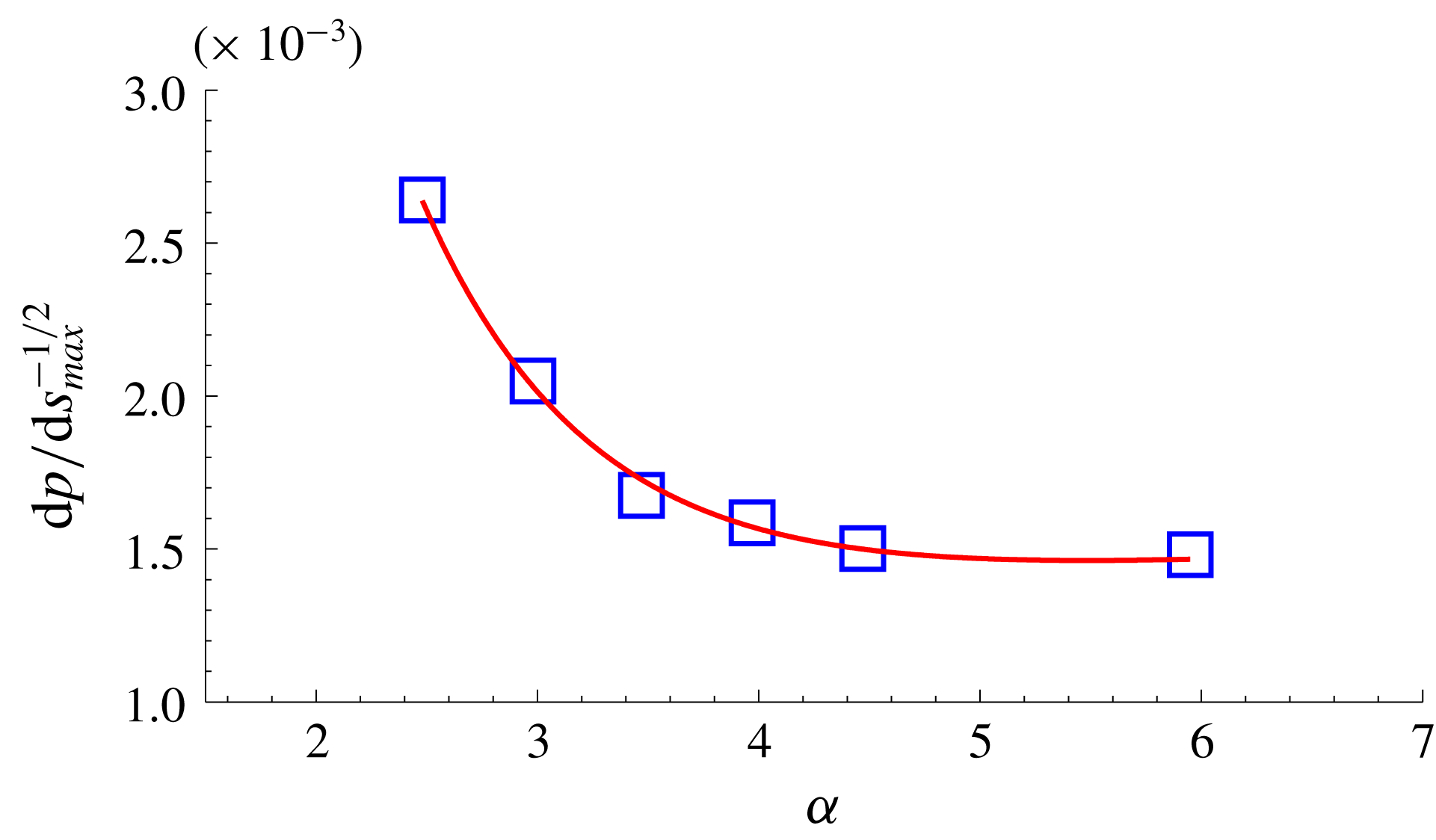
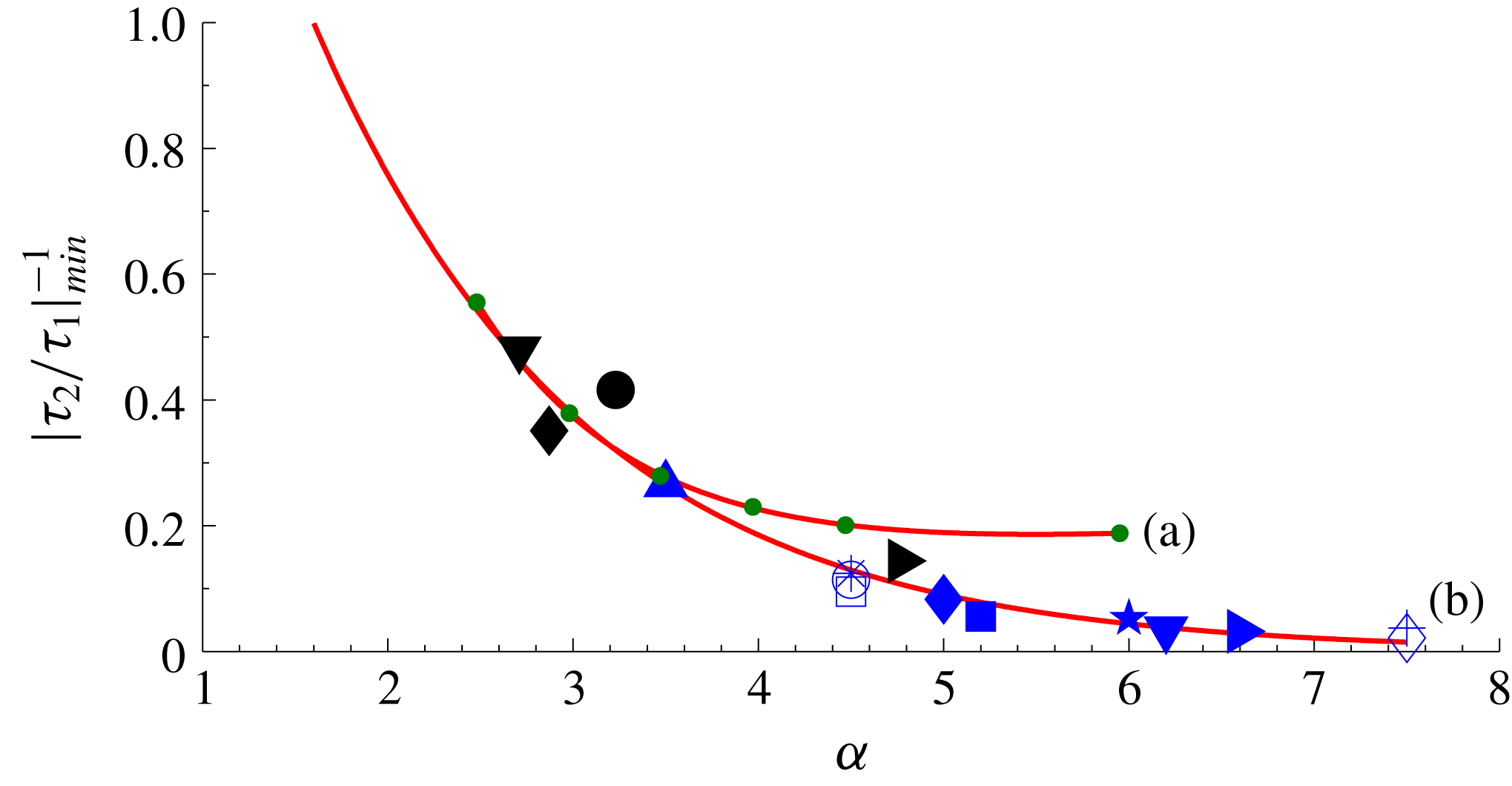
Figures 12 and 13 show the variation of the second shear stress minimum
 $|\unicode[STIX]{x1D70F}_{2}/\unicode[STIX]{x1D70F}_{1}|_{min}^{-1}$
and the maximum pressure gradient at reattachment
 $\text{d}p/\text{d}s_{max}^{-1/2}$
with scaled angle
 $\unicode[STIX]{x1D6FC}$
in the fashion of Smith & Khorrami (Reference Smith and Khorrami1991). The shear stress data in figure 12 show an increase in the magnitude of the minimum with increase in the scaled angle, and show virtually no significant change with
 $\unicode[STIX]{x1D6FC}>6$
. Similarly, maximum pressure gradient values in figure 13 show an exponential decay to a near constant value for
 $\unicode[STIX]{x1D6FC}>6$
. These changes in the magnitude of the second shear stress minimum and pressure gradient values with increase in the scaled angle for cold wall hypersonic separated flow are generally less severe than those in the Smith & Khorrami (Reference Smith and Khorrami1991) and Korolev et al. (Reference Korolev, Gajjar and Ruban2002) data because the Reynolds numbers in the present calculations are finite and moderate (of the order of
 $10^{5}$
) while the Smith & Khorrami (Reference Smith and Khorrami1991) and Korolev et al. (Reference Korolev, Gajjar and Ruban2002) solutions are asymptotically valid at large Reynolds numbers.
Variation of inverse of second minimum shear stress
 $|\unicode[STIX]{x1D70F}_{2}/\unicode[STIX]{x1D70F}_{1}|_{min}^{-1}$
with scaled angle
 $\unicode[STIX]{x1D6FC}$
. Symbols denote data points.

Variation of inverse pressure gradient
 $\text{d}p/\text{d}s_{max}^{-1/2}$
with scaled angle
 $\unicode[STIX]{x1D6FC}$
. Symbols denote data points.

The rapid changes in the separated region and the appearance of the secondary separation and its fragmentation with the increase of scaled angle have their origin in the reverse flow boundary layer and its separation. This was first pointed out by Neiland (Reference Neiland1970) and Stewartson (Reference Stewartson1975) and later discussed by Smith & Khorrami (Reference Smith and Khorrami1991), Neiland et al. (Reference Neiland, Sokolov and Shvedchenko2008) and Shvedchenko (Reference Shvedchenko2009). The reverse flow boundary layer which develops in the reattachment region progressively encounters an adverse pressure gradient as it grows in the reverse direction and ultimately separates giving rise to secondary separations and vortices. This in turn creates transverse pressure gradients across the separated region. See also the discussion by Korolev (Reference Korolev1991, Reference Korolev1992).
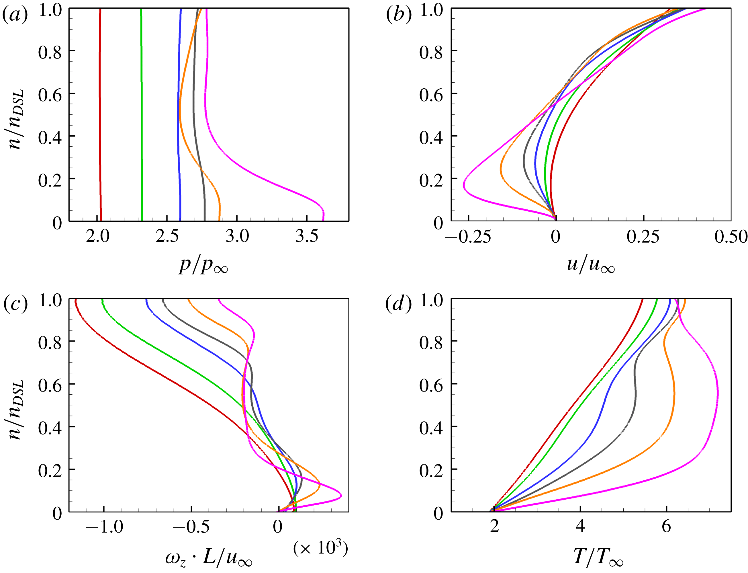
Figure 14 shows pressure (14
a), velocity (14
b), vorticity (14
c) and temperature (14
d) profiles for the reverse flow boundary layer region (see section A-A’ in figure 11), where
 $p$
,
 $u$
and
 $T$
are normalised by their corresponding free-stream values (subscript ‘
 $\infty$
’), while
 $\unicode[STIX]{x1D714}_{z}$
by
 $u_{\infty }/L$
, where
 $L$
is length of the flat plate. The figure shows these properties for all compression angles
 $10^{\circ }{-}24^{\circ }$
corresponding to scaled angles
 $\unicode[STIX]{x1D6FC}=2.47$
, 2.98, 3.47, 3.97, 4.47 and 5.95, respectively.
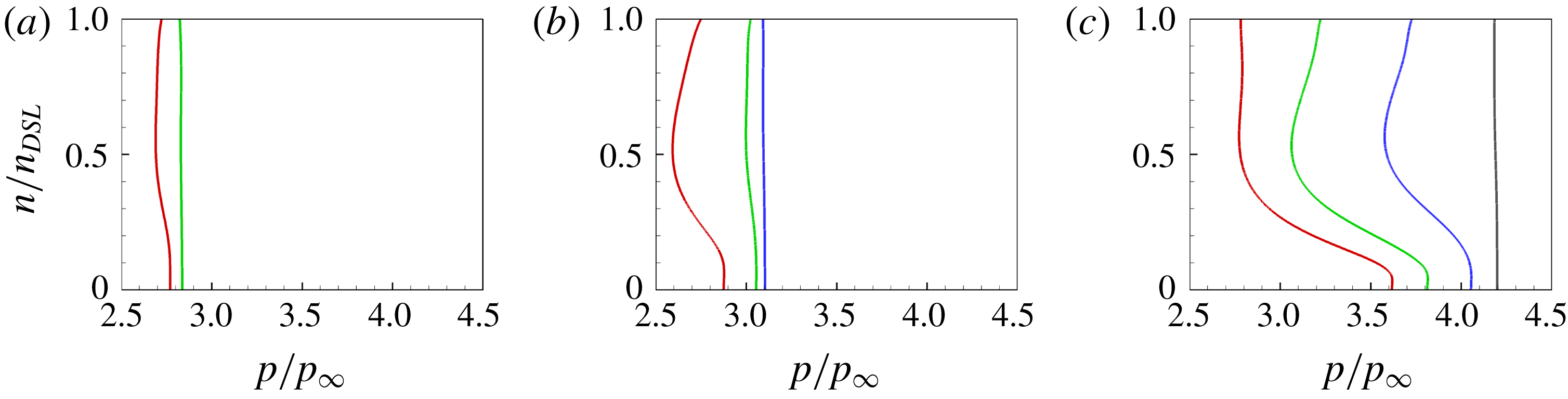
Considering pressure profiles first in figure 14(a), several features are noted. For angles up to
 $16^{\circ }$
, the pressure across the separated region is constant and, as discussed previously, secondary separation has not yet occurred. At
 $18^{\circ }$
angle (
 $\unicode[STIX]{x1D6FC}=3.97$
), however, we see a small pressure gradient near the surface in the transverse direction and as seen in figure 10, secondary separation has occurred. With
 $24^{\circ }$
angle (
 $\unicode[STIX]{x1D6FC}=5.95$
), we see a strong transverse pressure gradient in the separated region near the surface and severe fragmentation into secondary vortices has occurred (figure 10).
Reverse flow boundary layer (section A-A’ in figure 11) profiles in all compression angles. Transverse distance
 $n$
is normalised by the distance from the wall to the dividing streamline
 $n_{DSL}$
. Red:
 $10^{\circ }$
; green:
 $12^{\circ }$
; blue:
 $14^{\circ }$
; grey:
 $16^{\circ }$
; orange:
 $18^{\circ }$
; pink:
 $24^{\circ }$
. (a) Pressure; (b) velocity; (c) vorticity; (d) temperature.

Examination of the velocity profiles in figure 14(b) shows that with increasing angle, the primary separation size grows and when secondary separation begins to develop, we observe rapid variations in the reverse flow region near the surface and the profiles of
 $18^{\circ }$
and
 $24^{\circ }$
show inflection.
With regard to vorticity profiles in figure 14(c), up to
 $14^{\circ }$
, initially, the vorticity is zero indicating separation and convects rapidly into the outer region showing one large eddy. With increase in the angle, secondary separation develops as seen from changes in slope of the profiles in the transverse direction. These changes in the transverse direction are accentuated as the secondary separation and the fragmentation into vortices take place. It is also seen that vorticity maxima become sharper and there are rapid variations in vorticity in the transverse direction with increasing
 $\unicode[STIX]{x1D6FC}$
. Comparing the velocity and vorticity profiles in figures 14(b) and 14(c), it may be noted that vorticity maxima correspond to the inflection point in the corresponding velocity profiles.
Figure 14(c) shows temperature profiles. For each corner angle, the profiles indicate temperature through the main separated region and the vortices. Here for the lowest angle, there is a slight increase in temperature through the separated region but the temperature gradient at the surface shows no significant change for angles up to
 $16^{\circ }$
. With the increase in the angle, and the presence of secondary vortices, not only wall temperature gradients increase but also regions of high temperature within the reverse flow show an increase.
Transverse pressures at sections A-A’ to D-D’ (see figure 11) are shown in figure 15 for angles
 $16^{\circ }$
(15
a),
 $18^{\circ }$
(15
b) and
 $24^{\circ }$
(15
c). They elaborate further on transverse gradients at different locations of the separated region. Pressure profiles at these sections show that gradients do exist before the separation of each vortex and increase with the increase in deflection angle. The profiles also show that the gradients decrease away from the reattachment region (A-A’ to D-D’).
Pressure profiles at sections A-A’ to D-D’ (see figure 11) for angles
 $16^{\circ }{-}24^{\circ }$
. Transverse distance
 $n$
is normalised by the distance from the wall to the dividing streamline
 $n_{DSL}$
. Red: A-A’; green: B-B’; blue: C-C’; grey: D-D’. (a)
 $16^{\circ }$
; (b)
 $18^{\circ }$
; (c)
 $24^{\circ }$
.

4.3 Further remarks on the shear stress minimum
As discussed earlier, a significant feature of a large separated flow is the shear stress minimum immediately preceding reattachment. Secondly, this minimum is larger in magnitude than the one after separation. With increasing
 $\unicode[STIX]{x1D6FC}$
, this minimum becomes steeper and sharper when the Reynolds number is very large as asymptotically valid solutions of Smith & Khorrami (Reference Smith and Khorrami1991) and Korolev et al. (Reference Korolev, Gajjar and Ruban2002) have shown. Smith (Reference Smith1988) and Smith & Khorrami (Reference Smith and Khorrami1991) suggested that when the scaled angle
 $\unicode[STIX]{x1D6FC}$
is large enough, a stage may reach when
 $\unicode[STIX]{x1D70F}_{2,min}\rightarrow -\infty$
, a singularity. Subsequently, Korolev et al. (Reference Korolev, Gajjar and Ruban2002), based on Neiland’s (Reference Neiland1970) reattachment theory, found that their computations were smooth past the second minimum without encountering singularity for
 $\unicode[STIX]{x1D6FC}$
up to 7.5. These findings were also confirmed by Logue, Gajjar & Ruban (Reference Logue, Gajjar and Ruban2014).
To throw some light on this interesting feature of large separated flows, we have plotted the shear stress minimum
 $\unicode[STIX]{x1D70F}_{2}$
from available data in the literature, both numerical and experimental, against the scaled angle
 $\unicode[STIX]{x1D6FC}$
. It should be emphasised here that although some of these flows involved large separations (well-developed plateau), none discuss/comment on secondary separation or reverse boundary layer flow. As the various data (both compression corners and incident/ shock configuration) have been extracted directly from the quoted papers, some inaccuracies may likely have occurred and hence should be treated with caution. The trend, however, is quite clear.
Figure 16 shows the parameter
 $|\unicode[STIX]{x1D70F}_{2}/\unicode[STIX]{x1D70F}_{1}|_{min}^{-1}$
plotted against the scaled angle
 $\unicode[STIX]{x1D6FC}$
. Apart from the present hypersonic cold wall data (
 $T_{w}/T_{o}=0.125$
), all other data are adiabatic and supersonic. The Reynolds numbers are generally of the order of
 $10^{5}$
except those of the Smith & Khorrami (Reference Smith and Khorrami1991) and Korolev et al. (Reference Korolev, Gajjar and Ruban2002) data which are asymptotic solutions valid to
 $Re\rightarrow \infty$
.
Variation of
 $|\unicode[STIX]{x1D70F}_{2}/\unicode[STIX]{x1D70F}_{1}|_{min}^{-1}$
with scaled angle
 $\unicode[STIX]{x1D6FC}$
. Green dots in curve (a) present compression corner data for angles
 $10^{\circ }{-}24^{\circ }$
(
 $T_{w}/T_{o}=0.125$
). Curve (b) previous adiabatic wall data. (Black symbols: incident shock) ▾: Shrestha et al. (Reference Shrestha, Hildebrand, Dwivedi, Nichols, Jovanovic and Candler2016); ♦: Degrez, Boccadoro & Wendt (Reference Degrez, Boccadoro and Wendt1987); ●: Katzer (Reference Katzer1989); ▸: Yao et al. (Reference Yao, Krishnan, Sandham and Roberts2007). (Blue symbols: compression corner) ▴, ○, ▪, ▾ & ▸: Smith & Khorrami (Reference Smith and Khorrami1991); ▫, ♦,
 $\star$
& ♢: Logue et al. (Reference Logue, Gajjar and Ruban2014); * &
 $+$
: Korolev et al. (Reference Korolev, Gajjar and Ruban2002).

Considering the adiabatic wall data first, the trend from
 $\unicode[STIX]{x1D6FC}=2.5$
to 7.5 does show the second shear stress minimum
 $|\unicode[STIX]{x1D70F}_{2}/\unicode[STIX]{x1D70F}_{1}|_{min}^{-1}$
approaching zero for
 $\unicode[STIX]{x1D6FC}\approx 8$
. Smith & Khorrami (Reference Smith and Khorrami1994) have suggested a value ‘somewhat below 9’ for this critical value. These data are also consistent with the plateau appearing at
 $\unicode[STIX]{x1D6FC}\geqslant 2.5$
indicating ‘large’ separated flow and a well-developed plateau (Burggraf Reference Burggraf1975).
With respect to the present cold wall data, the first point to note is that the incipient separation angle is higher than the adiabatic value of 1.57. Secondly, with increasing
 $\unicode[STIX]{x1D6FC}$
, the fall in the shear stress minimum is more gradual, reaching a near constant value for
 $\unicode[STIX]{x1D6FC}\geqslant 6$
. For a small wall temperature ratio (
 $T_{w}/T_{o}\leqslant 0.3$
) and Reynolds number of the order of
 $10^{5}$
Shvedchenko (Reference Shvedchenko2009) shows that steady secondary separations occur when
 $\unicode[STIX]{x1D6FC}$
is between 5 and 6. He noted no secondary separation instabilities even at Reynolds number of the order of
 $10^{6}$
. His calculations do not extend beyond this value. This suggests that it is less likely that a critical value of
 $\unicode[STIX]{x1D6FC}$
exists for low wall temperature ratios. Our previous study of wall temperature effects on leading edge separation (Khraibut et al.
Reference Khraibut, Gai, Brown and Neely2017; Khraibut Reference Khraibut2018) are consistent with this view. Clearly, this is an area that needs further investigation.
4.4 Size of the separation bubble
Burggraf (Reference Burggraf1975) has shown that a large separated flow is characterised by
 $\unicode[STIX]{x1D6FC}\geqslant 2.5$
, and the bubble length scales as
 $\unicode[STIX]{x1D6FC}^{3/2}$
. Based on asymptotic theory, he proposed a relation for the plateau length
 $L_{p}$
as
 $$\begin{eqnarray}L_{p}=3.47(\unicode[STIX]{x1D6FC}-1.55)^{3/2},\end{eqnarray}$$
which is valid for
 $\unicode[STIX]{x1D6FC}\gg 1.55$
.
It should be pointed out here that, although the actual length of the separation region is slightly different from the length of the pressure plateau, they have been used synonymously in the literature. For example, Korolev et al. (Reference Korolev, Gajjar and Ruban2002) assume
 $l_{B}\sim \unicode[STIX]{x1D6FC}^{3/2}$
, where
 $l_{B}$
is the distance between separation and reattachment points. Rizzetta (Reference Rizzetta1976) also assumes the same for compression corner separation. In actual fact, the bubble length comprises the plateau length and a reattachment region of
 $O(lRe^{-1/2})$
just after the end of the plateau and before reattachment (see Burggraf Reference Burggraf1975 and Daniels Reference Daniels1979). In the present instance, we have taken the bubble length to vary as
 $\unicode[STIX]{x1D6FC}^{3/2}$
.
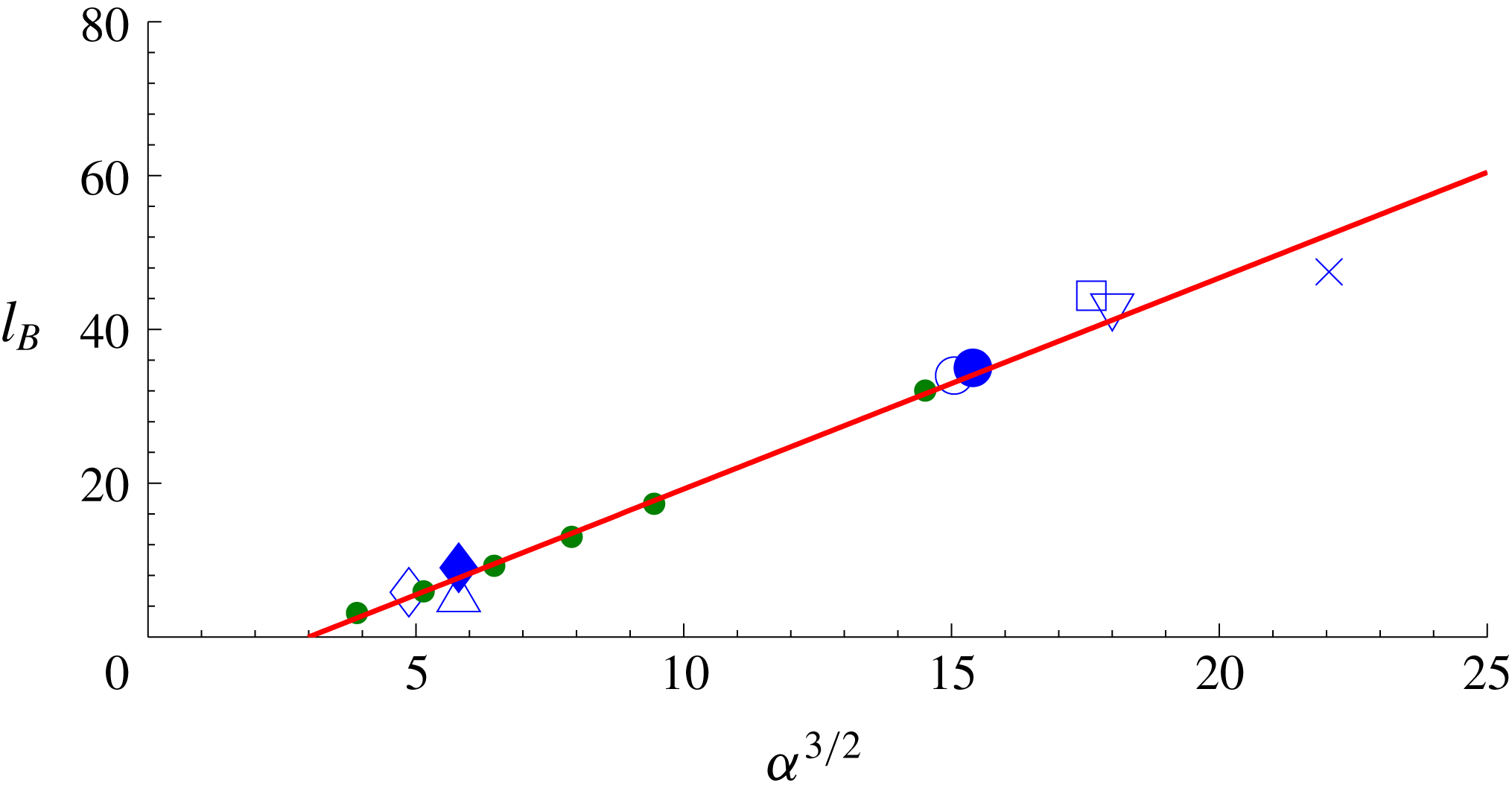
Burggraf (Reference Burggraf1975) also comments that there is a dearth of numerical solutions or experimental data to compare with his theoretical expression for separation bubble (plateau) length although he compares his theory with one of the Chapman et al. (Reference Chapman, Kuehn and Larson1958) experimental results, which showed reasonable agreement. Figure 17 shows the bubble length
 $l_{B}$
plotted against
 $\unicode[STIX]{x1D6FC}^{3/2}$
. The data correspond to compression corners, incident shock, leading edge separation and laminar axisymmetric SBLI. It is a linear relation with the zero intercept at
 $\unicode[STIX]{x1D6FC}\approx 2.5$
, which is when the plateau region develops. It shows that separation length is independent of the mode of generating large separations in line with the free-interaction concept. The data points shown here are estimated from the information provided from the quoted references, both numerical as well as experimental, and so may contain some inaccuracies but are believed adequate to draw conclusions. It is interesting to note this relationship seems also to be independent of wall temperature.
Variation of length of separation
 $l_{B}$
with scaled angle
 $\unicode[STIX]{x1D6FC}$
. Green dots: present compression corner data for angles
 $10^{\circ }{-}24^{\circ }$
(
 $T_{w}/T_{o}=0.125$
); ♢: Katzer (Reference Katzer1989) (adiabatic); ▵: Degrez et al. (Reference Degrez, Boccadoro and Wendt1987) (adiabatic); ♦: Rizzetta et al. (Reference Rizzetta, Burggraf and Jenson1978) (adiabatic); ○ & ●: Benay et al. (Reference Benay, Chanetz, Mangin, Vandomme and Perraud2006)
 $(T_{w}/T_{o}=0.6)$
; ▫: Khraibut et al. (Reference Khraibut, Gai, Brown and Neely2017)
 $(T_{w}/T_{o}=0.1)$
; ▿: Chapman et al. (Reference Chapman, Kuehn and Larson1958) (adiabatic);
 $\times$
: Swantek & Austin (Reference Swantek and Austin2012)
 $(T_{w}/T_{o}\approx 0.04)$
.

5 Conclusions
Large separated flows created with a flat plate compression corner geometry in hypersonic flow were investigated numerically and analysed. The characteristic features of large separated flows, a well-developed plateau region between separation and reattachment and appearance of secondary separation at large enough scaled angle have been studied and verified in high Mach number/moderate Reynolds number hypersonic flow. The conditions when secondary separation first appears and when fragmentation into multiple vortices occurs are identified in terms of the scaled angle
 $\unicode[STIX]{x1D6FC}$
and through detailed analysis of the reverse flow boundary layer and its separation.
Discussion of the second shear stress minimum and accompanying streamwise and transverse pressure gradients are discussed in the light of available (largely) supersonic adiabatic wall data and the present cold wall hypersonic data. While the available adiabatic wall data seem to indicate a critical scaled angle of approximately 8 as proposed by Smith (Reference Smith1988) for reversed flow singularity, the cold wall data did not show any tendency towards a critical angle.
It is shown that the size of the separated region is strongly dependent on the scaled angle being proportional to
 $\unicode[STIX]{x1D6FC}^{3/2}$
, in agreement with asymptotic expression of Burggraf (Reference Burggraf1975). It is also shown that this relationship is independent of the agency creating that separation. The relationship also appears to be independent of the wall temperature.
Acknowledgements
The authors are grateful to the Australian research Council for their support under grant DP-140100842. They would also like to thank National Computing Infrastructure (NCI) for providing computer resources. Sincere thanks are also due to Professor G. Candler of the University of Minnesota for permission to use the US3D code. The authors express their sincere thanks to the referees for their constructive comments and suggestions.