

1. Introduction
From the 1870s, Sweden, like other European countries, experienced what has been called a ‘grain invasion’ from America and Russia (O'Rourke Reference O'Rourke1997). The average yearly import of rye trebled from the 1860s to the 1880s, while that of wheat grew sixteen-fold. Between 1861 and 1870, only 11 per cent of the rye and 5 per cent of the wheat consumed in Sweden had been imported; by the 1880s, these shares had grown to 27 and 46 per cent, respectively (Lindahl et al. Reference Lindahl, Dahlgren and Kock1937, pp. 30ff.). Whereas a number of countries, notably Great Britain and Denmark, retained their free-trade orientation in the face of such pressures, Sweden joined France and Germany in imposing tariffs on agricultural and industrial imports. Kevin O'Rourke (O'Rourke Reference O'Rourke1997, pp. 778ff.) argued that where agriculture was concerned, the political choices of governments were related on the one hand to how the grain invasion affected land rents, and on the other to the weight of agricultural interests in domestic politics. As for Sweden, land rents appear to have been negatively affected by the shifts in the sectoral trade balances since the 1870s, and in reaction, interest groups demanding tariffs were formed (Esaiasson Reference Esaiasson1990, pp. 83ff.). The issue dominated two elections held in spring and autumn 1887. Both returned free-trade majorities. However, after the autumn election, the protectionists discovered that one of the members for Stockholm – who all supported free trade – had neglected to pay a negligible amount of his taxes. Electoral law not only disqualified this member but the other 22 members for Stockholm too. The votes cast for them were declared invalid, the protectionists gained a majority, and Sweden turned away from free trade.
In the face of similar developments in foreign trade, the German protectionists had carried all before them: in the general election of 1878 they had won a resounding victory, routing the free-trade-supporting liberals and changing the course of German politics for decades. Recent research has shown that unlike what has long been suspected, this was not primarily the result of political manipulation but rather a rational response of voters who feared for their livelihoods (Lehmann Reference Lehmann2010). Why did the Swedish protectionists make so little headway when their core issue came to the vote, and why did they have to resort to a legal sleight of hand to oust the free traders from power? Who voted for them, and which groups of voters continued to support free trade? And why did voters make the choices they made? These are the questions addressed in the present article.
There are several reasons why these questions are important and interesting. For one thing, the tariff debate was one of the most important political conflicts in modern Swedish history. It gave rise to the emergence of a ‘political mass market’ (to borrow a term coined for parallel developments in Imperial Germany; see Steinbach Reference Steinbach1990; Retallack Reference Retallack, Müller and Torp2009), where interest in political questions and participation in politics were more broadly and firmly established than before. Furthermore, the issue is not only important in the context of Swedish history in particular, but is relevant in general. This is the case because in Sweden as elsewhere, we can expect tariffs on imports to have affected different social and economic groups in different ways. At the most basic level, industrial tariffs benefited capital owners and agricultural tariffs farmers, whereas all other groups suffered from the rising prices; but this is only the broadest picture. Agriculture was nowhere homogeneous; farm size and the degree and type of specialisation complicate the issue.Footnote 1 Thus, large landowners who regularly supplied grain to the market would gain from protection, whereas smallholders may have produced for home consumption only. Tariffs would then not affect them. Likewise, farmers specialising in the production of wheat or rye naturally benefited from protection, but others, who specialised in animal husbandry, may have needed to buy grain as fodder; consequently tariffs would harm them.
As for prior research, studies that aim at answering questions concerning the link between commercial policy interests and voting behaviour have repeatedly been undertaken in the context of late nineteenth-century history (e.g. Klug Reference Klug2001; Van Dijck and Truyts Reference Van Dijck and Truyts2010). However, most of them used traditional econometric approaches such as simple logistic or probit regressions that, when applied to voting, can produce problematic results. Modern election analysis offers tools which produce far superior estimates. The most important of these methods is King's algorithm, on which the analysis presented in this article is based. The algorithm provides point estimates and confidence intervals for the votes of different groups of voters for every constituency. It extracts much more information from the available data than simpler methods. King's algorithm is introduced in detail below; for the present, suffice to say that the method here applied is superior to older approaches.
To date, there are only two historical cases where King's algorithm has been applied: Gary King et al. (Reference King, Rosen, Tanner and Wagner2008) examined Weimar Germany in order to show who voted for Hitler, and Sibylle Lehmann (Reference Lehmann2010) analysed elections in Imperial Germany to determine which groups of voters were responsible for the country's turn to protectionism. Swedish nineteenth-century elections have never been studied from this perspective, and have in general received little attention. Arthur Montgomery (Reference Montgomery1921, pp. 135ff.) discussed the two elections of 1887 in his account of Swedish tariff policies, but he provided few data and did not attempt a systematic breakdown of who voted for whom. It was Elis Håstad (Reference Håstad1941) who laid the groundwork for future analyses by determining the political affiliations of the candidates in the two elections of 1887 and in the one of 1890. Leif Lewin et al. (Reference Lewin, Jansson and Soerbom1976) estimated the impact of the social structure on voting behaviour in the period from 1887 to 1968. This is the only quantitative attempt to investigate the electorate and its voting behaviour in Sweden. Lewin et al.'s work provides a good overview of the electorate but is not detailed enough to compare the voting behaviour of different categories of farmers and of other occupations with expectations derived from trade models or empirical results. The authors grouped occupations with similar voting behaviour and analysed this for just four extracted groups. Some political scientists, for instance Peter Esaiasson (Reference Esaiasson1990), have studied electoral campaigns during this period, but in a rather descriptive way. With regard to trade policy, Jan Bohlin (Reference Bohlin2005; Reference Bohlin2009) focused on the actual effective tariff protection in the late nineteenth and early twentieth centuries, and the impact of tariffs on the income of different groups of farmers. How the decision to introduce tariffs came about, and how the electorate voted in this context, are issues outside the scope of his research. These are questions that the available data and modern methodology allow us to analyse in much more detail than prior research has been able to do.
The rest of the article is organised as follows. In Section 2 we provide an overview of Swedish electoral law. In the following section, we take a closer look at the voters, examining how their commercial policy interests were formed and what shape these interests had. Following this, we present our analysis and its results (Section 4), and a final section concludes.
2. The Swedish electoral system
At the time of the tariffs debates, Sweden had a two-chamber system where a law had to be accepted in both chambers by a simple majority (Verney Reference Verney1957, pp. 50ff.; Särlvik Reference Särlvik, Grofman and Lijphart2002, pp. 232f.). The First Chamber was elected by the councils of the provinces (läns) and by cities outside the provinces; it does not concern us here. The Second Chamber was more popular in character; it was elected in general elections by all enfranchised citizens. However, in late nineteenth-century Sweden the franchise was still severely restricted. The electoral law passed in 1866 and valid until the reform bill of 1907 stipulated that voters had either to own real estate of a taxable value of at least 1,000 Kronor, or to have leased farm property whose taxable value exceeded 6,000 Kronor for at least five years, or paid taxes on an income of at least 800 Kronor p.c. a year.Footnote 2 In 1885, there were about 330,000 enfranchised persons in Sweden, almost 240,000 of whom had gained the right to vote because they owned estates. Only about 11,000 were leaseholders, and fewer than 80,000 owed their voting right to their income. In the different constituencies, the rate of enfranchisement varied between around 3 and just over 10 per cent of the population (BISOS 1885, pp. 74f.; BISOS 1887, pp. xivff., 230).
The constituencies were formed on the basis of the administrative units below the provinces (called härad, domsaga or fögderi), with most consisting of between one and five such districts. The aim was to form single constituencies of about 40,000 inhabitants each. Towns composed their own constituencies. Those with a population of 10,000 or more formed one each where one member was elected for every 10,000 residents, while smaller towns could group together and form separate constituencies, electing one member for every 6,000 inhabitants (Verney Reference Verney1957, pp. 52f). This measure seems to have been designed in order to make up for the smaller share of persons entitled to vote in small towns. In 1885, on average 1,700 eligible voters were registered per constituency (BISOS 1885, pp. 46ff.). Altogether, there were 186 constituencies, 41 of which were urban. The law of 1866 created a mixed system of direct and indirect elections. Voting was to be direct in towns that returned members of their own and indirect where a large constituency was formed by a group of districts or small towns. However, districts and small towns could choose to elect members directly, which they increasingly did (Verney Reference Verney1957, pp. 53). By spring 1887, only 60 indirect constituencies were left; by autumn, that number had fallen to 41 (Caramani Reference Caramani2000). In some of these voting seems to have been open – making instances of group and other pressures more likely –, but elsewhere it was always by secret ballot (Särlvik Reference Särlvik, Grofman and Lijphart2002, p. 232).
The electoral law also stipulated that elections had to be held every three years regardless of additional elections that might have to take place in between due to the dissolution of parliament by the king. Actually, this is what happened in 1887 (Verney Reference Verney1957, pp. 106f.). In the years before, the protectionists had gradually gained ground in the First Chamber, and a first law in favour of tariffs had been passed in the Second Chamber. Before a joint vote could be taken, King Oskar II – pleased to be able to demonstrate his political power and to use his dissolution prerogative – dissolved parliament. The government that had suggested this measure aimed at achieving a clearer picture about public opinion (Anderson Reference Anderson1955/70, pp. 373f.). In consequence, an extraordinary election in March 1887 became necessary, but the regular election of autumn 1887 was held regardless.
Both elections of that year were overshadowed by the tariff issue to such a degree that they more closely resembled referenda about tariffs. Campaigning in spring of 1887 was intense, with statements about the tariff question dominating. Many candidates published so-called ‘political confessions’ in local newspapers, in which they stated whether they were free trade or tariff supporters (Esaiasson Reference Esaiasson1990). Another new trend was the appearance of interest groups all over the country, for instance the ‘Friends of Swedish Work’ who demanded specific tariffs, and the ‘Union against Food Tariffs’, whose members favoured free trade. Most of these organisations were founded by parliamentarians (Esaiasson Reference Esaiasson1990, pp. 83ff.). Initially, there was a huge upsurge in interest. Overall turnout increased from around 26 per cent of the eligible voters in 1884 to more than 66 per cent in spring 1887, with participation in rural areas, where involvement in political discussions was usually weak, growing particularly strongly. By autumn, however, a certain voter fatigue could be observed. Average turnout fell to around 37 per cent, rural turnout to 32 per cent (Caramani Reference Caramani2000).
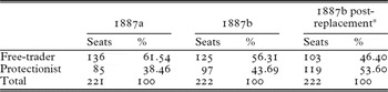
The way the results of these elections were reported to the public differed from that of later contests. Political parties were only beginning to develop in late nineteenth-century Sweden (Verney Reference Verney1957, pp. 98ff.). In consequence, national statistics do not give the results by party, but rather the names of the candidates and the numbers of votes they received (BISOS 1888, pp. 45ff.). In order to determine how the electorate voted in spring and autumn 1887, it is therefore necessary to establish the political leaning of each individual member elected to parliament. This has been done on the basis of public statements, brochures and newspaper reports, which contain sufficient information to allow the identification of each candidate as either free-trade supporting or protectionist (Håstad Reference Håstad1941). Table 1 provides an overview of the results.
Results of the Swedish general elections 1887

Source: Håstad (Reference Håstad1941).
*Results after the replacement in the Stockholm parliaments.
As a result of the tax scandal described in the introduction, a protectionist majority was established.Footnote 3 This majority formed a new government, and in 1888 tariffs were introduced for a number of agricultural and industrial products (Bohlin Reference Bohlin2005).
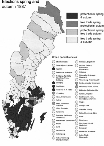
Despite the consistent free-trade majority that the elections of 1887 showed, there were interesting shifts between spring and autumn, and interesting regional differences. Figure 1 shows the geographic distribution of the electorate's preferences.
The results of the general elections of 1887

Practically the whole country north of Uppsalas län was firmly pro free trade, and free traders had further strongholds in Malmöhus and Halland. The protectionists, by contrast, were strong in the rest of the south and on the islands of Öland and Gotland.
3. Commercial policy interests and their determinants
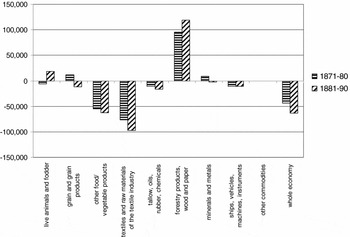
The interests voters developed in the field of commercial policies were shaped by how exports and imports affected their incomes. Accordingly, to determine these interests we first need to examine the structure of Sweden's foreign trade in the late nineteenth century. Recent research (Bohlin Reference Bohlin2007, p. 18) has found that in the mid 1880s, i.e. before the newly introduced tariffs caused a marked shift in the structure of trade, the Swedish capital goods industry had an import penetration ratio of 23 per cent, the consumer goods industry one of 44 per cent, the food industry one of 24 per cent and agriculture one of 10 per cent, but such aggregates obscure the details which we are primarily interested in. More specifically, at this time grain, timber and forestry products dominated exports, while the foremost import commodities were agricultural and food products, textiles and cloth (Bohlin Reference Bohlin2007, p. 4). Figure 2 gives an overview of the sectoral trade balances, allowing a comparison between the averages of the 1870s and 1880s.
Swedish trade balances by sector in 1000 Kronor, 1871–80 and 1881–90

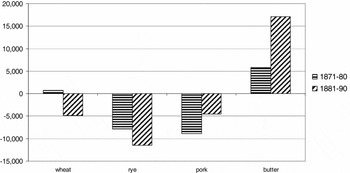
The figure shows not only that the Swedish economy as a whole suffered from an adverse balance of trade, but also that the situation of most economic sectors worsened from the 1870s to the 1880s. There were only two at least partial exceptions: forestry did well over the whole period, and the balance of trade of live animals and animal fodder turned positive in the 1880s. In our analysis, we do not neglect the other sectors, but our focus is on agricultural voters. There are two reasons for this. First, the majority of the population and voters were working in this sector. In 1887 they constituted roughly 65 per cent of the entire working population (Lindahl et al. Reference Lindahl, Dahlgren and Kock1937, p. 2). Second, because land is an immobile factor of production, we can define the tariff political interests of farmers in regional terms. By contrast, when we try to determine the interests of capital owners, mobility is a problem: we cannot be sure if they cast their votes at the place where they invested their assets. In consequence, constituencies with capital-intensive industries did not necessarily have voters who received the main part of their income from capital returns. The voters whose behaviour we analyse were therefore farmers of different types, i.e. farmers who worked estates of different sizes and were specialised in different ways. Commercial developments in the 1870s and 1880s affected these subsectors of agriculture in different ways. Figure 3 shows how the trade balances of the four most important products developed.
Agricultural trade balances in 1000 Kronor, 1871–80 and 1881–90

Obviously, and in accordance with what the ‘grain invasion’ hypothesis implies, farmers specialising in the production of wheat and rye were hit hardest by the increase in long-distance trade in staples that was part and parcel of the ‘first wave of globalisation’ (see Foreman-Peck Reference Foreman-Peck1998). The position of pork farmers improved, and butter became an important export commodity from the 1880s (see Bohlin Reference Bohlin2007, p. 4). In so far as producers wanting to shift their assets from wheat or rye, for example, to cattle farming faced costs, this suggests that specialised grain farmers should have favoured protection to a far higher degree than farmers who specialised in the production of pork or dairy products.
We ask, primarily, if this was the case, or more generally, how the distribution of voters and votes that were cast in the elections in 1887 related to these commercial policy interests. Unfortunately, Swedish national statistics do not provide data on the agricultural specialisation of the voters. What they do provide is detailed information on the value of the estates that the voters held (BISOS 1885, pp. 46ff.). Relating this information to Swedish land values from 1887 (Lindahl et al. Reference Lindahl, Dahlgren and Kock1937, p. 393) allows us to estimate the size of the farms owned or leased by the voters. In addition, we can use constituency-level data on the area of farmland on the one hand, and on the output of wheat and rye and on the numbers of dairy cows and pigs on the other (BISOS 1890).
Bohlin (Reference Bohlin2009, p. 12), who examined the long-term income distributional effects of the tariffs introduced since the late 1880s, found a close match between farm size and specialisation: the larger the farm, the higher the degree of specialisation in bread grain production. He used detailed post-World War I data on the output mix of farms of different sizes (Höijer Reference Höijer1921). Still, we can not simply assume that his results hold for our period too. One of Bohlin's (Reference Bohlin2009, pp. 7f.) core hypotheses is that owing to the high income elasticity of demand for meat and dairy products and the strong export demand in particular for butter, Swedish agriculture experienced an ongoing transformation in the direction of more animal produce in the late nineteenth and early twentieth centuries. In 1887, livestock farming was clearly less important than thirty years later. However, how important was it? Where was it concentrated, and can we relate its geographical concentration to free-trade strongholds?
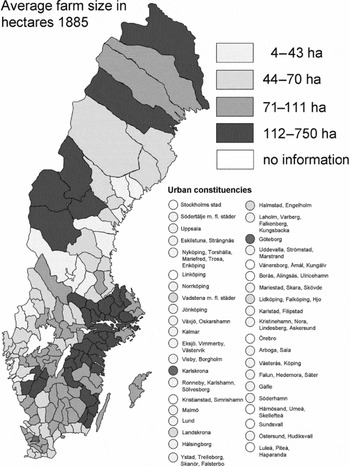
Figure 4 shows the geographical distribution of farm sizes. The map is based on data collected in 1888 (BISOS 1890), i.e. early enough for the introduction of tariffs not to have affected the sectoral structure.
Farm sizes (excluding managed and unmanaged woodland)

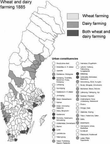
Farm sizes differed clearly between regions. Large estates existed in the neighbourhood of cities such as Stockholm, Kalmar and Göteborg and in densely urbanised Södermans län and Östergotland; in the north-west and extreme north of Sweden farms were also large. By contrast, smaller farms and smallholdings prevailed in less densely urbanised and more marginal parts of the country, i.e. in parts of the south and in central Sweden. As for bread grain production, we are considering the quantities of wheat and rye produced per hectare of agriculturally used land, which is defined as land used as garden, arable and pasture (BISOS 1890). Thus, we assume it excludes both managed and unmanaged woodland. Wheat farming was concentrated around Stockholm, in Södermans län and in Malmöhus. In the north, owing to climatic conditions, it hardly occurred, but it was also of minor importance in many southern regions, e.g. in Kronobergs län. Rye farming too was very rare in the north, being concentrated in central Sweden and in the coastal districts of the south-east. Estimating the numbers of cows per hectare of farmland shows that dairy farming was more unevenly distributed. Dairy farming was strong in central Sweden, on parts of the west coast and in the extreme south-east of the country. Figure 5 shows the 30 per cent of the constituencies where the output of wheat and the number of cows per hectare farmland was highest, respectively.
Constituencies dominated by wheat and dairy farming

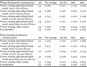
While a geographical representation shows a vague association of farm size and specialisation – where farms were large, farmers seem to have produced more wheat; where holdings were small, they appear to have had more cows per unit of land – Table 2 shows the link more clearly. We picked the same constituencies that are shown in Figure 5 and analysed the distribution of farm values and types of properties owned or leased by the voters. Obviously, due to the restricted suffrage, smaller landholdings are underrepresented here, because owners of theses estates were excluded from voting.
Overview: structure of voters owning farms in the wheat- and dairy-dominated constituencies

Note: The statistics report two types of land, agricultural land and other land respectively. We assume that agricultural land excludes woodlands. The category ‘wheat-dominated constituencies’ is defined as the 30 per cent of the constituencies with the highest wheat output per hectare agricultural land. The category ‘dairy-farming-dominated constituencies’ is defined as the 30 per cent of the constituencies where the density of cows per farmland was highest.
Source: BISOS (1890).
As for bread grain farming, we consider wheat because in the course of the grain invasion the growth in imports affected producers of wheat more severely than producers of rye (see above). We examine 54 constituencies, i.e. the 30 per cent with the highest wheat output per hectare of agricultural land. Owing to the availability of data, in the case of dairy farming the 30 per cent consist of the 52 constituencies where the number of cows per hectare of farmland was highest. Both in the case of wheat production and in that of dairy farming, a high proportion of the voters held farms of medium size, having a value between 2,000 and 10,000 Kronor (27 and 33 per cent, respectively). However, where wheat farming dominated, voters from small farms were rarer (8 per cent) than where farms focused on dairy production (10 per cent). By contrast, voters with large farms, whose value exceeded 10,000 Kronor, were more common in constituencies where wheat was produced than in those where farmers held cattle (14 vs 8 per cent). Leaseholders and owners of land that the Swedish national statistics classified as non-agricultural have been included for the sake of completeness. Altogether, we can conclude that the tendency of large estates to specialise in bread grain production while smallholdings focused on animal husbandry, which Bohlin (Reference Bohlin2009) established on the basis of post-World War I data, was already evident at the end of the 1880s. Given these results, we would expect voters who owned large farms to favour protection and smallholders to prefer free trade – in other words, we are able to use farm sizes as an indicator of the specialisation and political views of the voters.
4. Who voted for whom, and why?
4.1. The problem of ecological inference
Our analysis proceeds in four steps: first, we discuss a problem that commonly besets election analyses such as ours – that of ecological inference – then we provide some general information and descriptive statistics. Thereafter we analyse the data with the help of King's algorithm and, finally, we check and refine our results with robustness checks, for instance from a more traditional approach – Goodman's regression.
In the introduction, we briefly mentioned the ecological inference problem and promised a detailed discussion. This is indeed necessary as ecological inference commonly biases analyses such as ours. The nature of this problem can in fact very well be explained on the basis of our data. Thus, we know how many votes were cast for free-trade-supporting candidates and how many for protectionists in the Swedish elections of 1887, and we can estimate how many voters were dairy and how many wheat farmers.Footnote 4 This information is available for every constituency. What we are interested in is the voting behaviour of individuals, or at least of sub-aggregates, for example how many farmers with farms between 2.3 and 4.6 hectares – i.e. those from the lowest property bracket – voted for free trade in a particular constituency. Why is answering such a question a problem? Assume that in one constituency, 30 per cent of the electorate consisted of those dairy farmers and that 30 per cent of the votes were cast for candidates who supported free trade. In another constituency, 40 per cent of the electorate consisted of such farmers and 40 per cent of votes were cast for free-trade-supporting candidates. It thus seems that there is a perfect positive correlation of farmers with farms between 2.3 and 4.6 hectares and votes for free trade. However, regardless of how intuitive this relationship may be, farmers with farms between 2.3 and 4.6 hectares may actually not have voted for free trade at all. The votes for free trade may have come from industrial workers, who could conceivably favour free-trade-supporting candidates in constituencies dominated by agriculture. Hypothesising about the behaviour of individuals by using aggregate data can therefore be misleading: it means making inferences without considering the social environment of the individuals concerned. This is why it is called a problem of ecological inference. It is well known in political science: William Ogburn and Inez Goltra (Reference Ogburn and Goltra1919) introduced it in the very first multivariate statistical analysis ever to have been published in a political science journal, and it has been among the longest-standing unsolved problems in quantitative social science (King Reference King1997).
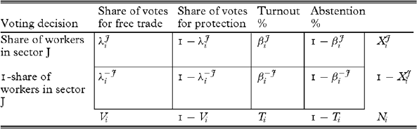
Table 3 shows how the problem can be illustrated in a formal manner. Suppose we want to find out whether or not workers in a specific sector voted for parties that supported free trade. The table shows the problem for one constituency and for two groups of voters, i.e. for those favouring free trade and protection, respectively. Here the workers employed in sector J are the voters of interest.
The ecological inference problem for constituency i and occupation J
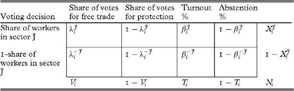
Note: xJi is the share of the workforce in constituency i employed in sector J. This could be, for example, the share of farmers. Vi is the share of votes for free-trade-supporting parties in the constituency i and 1−Vi the share of votes for parties that support protection. Ti is the percentage turnout. These values are known. The unknown quantities of interest are: λJi, which is the share of workers in sector J in the constituency i that voted for free ; λ−Ji, which is the share of workers of sectors outside J that voted for free trade; βJi, which is the turnout of the workers in sector J in the constituency i; and β−Ji, which is the turnout of workers in other sectors.
For every constituency, national statistics provide the values in the margins of the table, where index i indicates constituency i, and J indicates sector J. xJi is the share of the workforce in constituency i employed in sector J. This could be, for example, the share of farmers with between 2.3 and 4.6 hectares constituency i. Vi is the share of votes for free-trade-supporting parties in constituency i and 1−Vi the share of votes for parties that support protection. Ti is the percentage turnout for constituency i. What these statistics do not show, however, are the values in the inner (framed) cells of the table, such as the shares of various occupations in a particular constituency that voted for free trade, for protection, or abstained; that is the λi's and βi’s, which are not directly observed. λJi is the share of workers in sector J in constituency I, who voted for free trade and 1−λJi is the share of workers of sector J who voted for protection. For example, assuming that J is the agricultural sector, λJi is the share of farmers who voted for free trade and 1−λJi the share of farmers who voted for protection. Similarly, λ−Jiis the share of non-agricultural workers who voted for free trade, and 1−λ−Ji is the share of non-agricultural workers who voted for protection. βJi is the turnout of the workers in sector J in the constituency i. Clearly these parameters are the really relevant ones. If we can estimate these values, we obtain far more and better information about the voting behaviour of different sectors or, in our case, groups of farmers with different specialisations, than with the help of other approaches.
4.2. King's algorithm
The most advanced and modern tool for election analysis, and the only one that allows us to solve the ecological inference problem, is King's algorithm. King (Reference King1997) starts out from an equation introduced by Leo GoodmanFootnote 5 (Reference Goodman1953) into election analysis (equation 1), but combines it with the ‘method of bounds’. The ‘method of bounds’ derives from the observation that we can deterministically put some limits on individual behaviour from the available aggregate data. Assume for instance that we observe two types of voters (wheat and dairy farmers) and two voting options (voting or not voting). The turnout in constituency i (Ti) is just the proportion of wheat farmers who voted in this district (βJi) times the share of wheat farmers in constituency i (Xi), plus the proportion of dairy farmers who voted multiplied by the share of dairy farmers in this constituency:

Since we know the turnout, the true proportions of voters among wheat and dairy farmers must fall somewhere on a downward sloping line, whose slope is determined by the ratio of wheat farmers to dairy farmers, and whose intercepts will depend on the turnout as well:
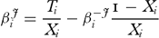
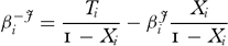
If we had only one set of aggregate data, for example information on the turnout and the share of farmers for the whole of Sweden, this would be as far as we could go, but we have aggregate data for every constituency. Each set of aggregate data, that is, each constituency, gives us such a line. They can all be drawn in one so-called tomography plot. This is informative, but does not provide enough information to get a clear solution. There is no exact way of recovering the values in the inner cells of Table 3. The simplest assumption to start with is that the true proportions for each constituency are picked at random from some distribution, but that all constituencies are drawn from the same population. King focuses on the case where that distribution fits the joint probabilities to a truncated bivariate normal distribution so that all proportions are between 0 and 1. In order to get the parameters from the truncated bivariate normal distribution, King uses the lines from the above-mentioned plot. The normality assumption helps detect the mode on the tomography plot, where most of the lines cross, and improves estimates by ‘borrowing strength’ from other constituencies. Intuitively, the most likely values for βJi and β−Ji are nearest the mode. Adding a couple of modest assumptions, five intermediate parameters that define the truncated bivariate distribution are estimated via a maximum likelihood function. The parameters are then transformed and rescaled. The means of the distribution of βJi and β−Ji are used as point estimates, and standard errors are based upon the variation in the simulated values. Thus King's algorithm provides sub-estimates for every constituency and thereby extracts much more information from the available data than simpler econometric tools.
Furthermore, one can use additional information as control variables to ensure the quality of the estimation. Here, we use a dummy variable that indicates urban constituencies for this purpose. If chosen correctly, such a variable will control for ‘aggregation bias’. Aggregation bias occurs if the variation of the parameters βJi and β−Ji or λJi and λ−Ji in specific areas differs from the general pattern of the aggregated constituency. One simple example will clarify this. Assume that at the individual level, the turnout of dairy farmers systematically exceeds that of wheat farmers. Further assume that one can observe a positive correlation between the turnout and the share of wheat farmers, if plotted for all constituencies. This implies that, if the proportion of wheat farmers increases, the turnout increases as well. The mistaken ecological inference is that wheat farmers vote at higher levels than dairy farmers. If this problem occurs one can choose control variables, which explain the rise in turnout (see King Reference King1997, p. 288). A description of the methods used to estimate these parameters is beyond the scope of this article; the interested reader is referred to King (Reference King1997) for more details.Footnote 6
4.3. Descriptive statistics
As mentioned above, national statistics do not give the results by party, but the names of the candidates and the numbers of votes they received (BISOS 1888, pp. 45ff.). The political leaning of each individual member elected to parliament was determined by Håstad (Reference Håstad1941). Based on this information we calculate the share of votes for free trade and the share of votes for protectionism for all constituencies. Furthermore, national statistics provide data for the electorate in the year 1885 at the level of constituencies. Since the suffrage was restricted to voters who owned a certain amount of land or received a certain income, the data do provide information about property and income (BISOS 1890).
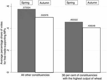
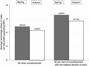
As discussed above, we assume that voters in constituencies dominated by smaller farms, and therefore rather specialised in animal husbandry, should be more in favour of free trade, while constituencies dominated by large farms (mainly wheat producers) should be in favour of protection. The following figures provide some descriptive statistics of voting for free trade for constituencies dominated by small farms and large farms and by highest wheat production and highest cow density to give a first overview of voting patterns.
Figure 6 shows the average percentage share of votes for free-trade-supporting MPs for the 30 per cent of constituencies with the largest wheat output compared to the other 70 per cent. The figure supports our hypotheses: constituencies where more wheat was produced had on average a lower share of votes for free-trade-supporting MPs than all other constituencies. The majority of voters in theses constituencies voted for MPs in favour of protection.
Average percentage share of votes for free-trade-supporting MPs for the 30 percent of constituencies with the largest wheat output

Figure 7 shows the same graph, now split into the 30 per cent of constituencies with the highest density of cows per hectare and the rest. It supports our hypothesis that farmers who were more specialised in milk production and animal husbandry were more in favour of free trade, since the average percentage share of votes for free trade was higher in constituencies with a higher density of cows.
Average percentage share of votes for free-trade-supporting MPs for the 30 per cent of constituencies with the highest density of cows

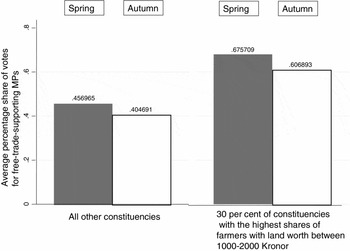
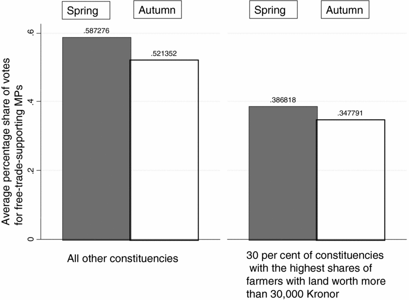
Figure 8 shows bar charts for the percentage share of votes for free trade for the 30 per cent of constituencies with the largest shares of smallholders, i.e. farmers owning land between 1,000 and 2,000 Kronor, and Figure 9 shows the same bar chart for the constituencies with the richest farmers in our sample, i.e. those who owned land worth more than 30,000 Kronor. In each figure we provide the average votes for free trade for the other constituencies as comparison group.
Average percentage share of votes for free-trade-supporting MPs for the 30 per cent of constituencies with the highest share of farmers owning land worth between 1000 and 2000 Kronor

Average percentage share of votes for free-trade-supporting MPs for the 30 per cent of constituencies with the highest share of farmers owning land worth more than 30,000 Kronor
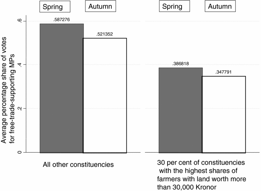
Here again, there is much support for our hypotheses. The 30 per cent of constituencies with the highest share of farmers owning smallholdings worth between 1,000 and 2,000 Kronor were rather in support of free trade, whereas the 30 per cent of constituencies with the highest share of rich farmers favoured protection to a far higher degree. However, as explained above, these correlations might be biased by the problem of ecological inference.
4.4. Main results
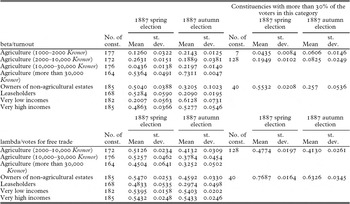
As mentioned above, owing to the lack of primary data on the agricultural specialisation of the voters, we do not use the shares of wheat and dairy farmers, but those of voters from different income groups and owning estates of different values. Table 4 reports the results for beta (turnout) and lambda (votes for free trade) estimated with King's algorithm. On the left, the results are shown for all constituencies; on the right, for those constituencies where the several groups of voters made up more than 30 per cent of the electorate. This was nowhere the case for voters who owned farms of between 10,000 and 30,000 Kronor, for leaseholders and for voters who owed their right to vote to their income. As the geographical location of the voters here does not concern us, we can include at least part of these voters in the analysis. Our assumption is that those in the lowest income bracket (800 to 1,000 Kronor) reported in the national statistics earned wages, whereas those in the highest bracket (more than 5,000 Kronor) derived their income from capital.
King's estimates for beta/turnout and lambda/votes for free trade

The results shown in Table 4 evidence that generally turnout was quiet low, particularly so for farmers with very little land and farmers with estates whose value exceeded the average (10,000 to 30,000 Kronor). However, among smallholders turnout increased between spring and autumn 1887. It also increased among richer estate owners (more than 10,000 Kronor), but fell off among middling farmers (2000 to 10,000 Kronor). This decline is even more obvious when we consider separately the 128 constituencies where such middling farmers made up more than 30 per cent of the electorate.
As for lambda, i.e. free-trade support, both groups of voters who had the right to vote because they earned a yearly income of about 800 Kronor (very low incomes) had a slight preference for free trade. This did not change appreciably between spring and autumn 1887. Obviously, low-income wage earners were opposed to agricultural protection because this would have increased the price of food. The behaviour of high-income capitalists fits expectations derived from Bohlin's (Reference Bohlin2009, pp. 33f.) analysis of the impact of tariffs: agricultural tariffs harmed the members of this group too. In contrast to them, the agricultural sector did not vote homogeneously. In spring 1887, smallholders preferred free trade – even more so in regions where they were very concentrated, constituting more than 30 per cent of the voters. Large landowners, by contrast, preferred protection. However, in the autumn election the picture changed slightly, with smallholders beginning to turn away from free trade. Such changes are unsurprising and conform, in fact, to a well-known and frequently researched pattern (see Ferejohn Reference Ferejohn1986; Abramowitz et al. Reference Abramowitz, Cover and Norpoth1986; Anderson and Ward Reference Anderson and Ward1996): an incumbent party tends to loose votes in an election that closely follows the one that brought it to power. However, the losses that the free traders suffered might also indicate electoral manipulation in constituencies where large landowners were able to put pressure on smallholders (electoral manipulation has recently received increasing attention; see, for example, Alston and Gallo Reference Alston and Gallo2010). Though anecdotal evidence for this hypothesis does not seem to exist, we are still going to return to it later in our analysis.
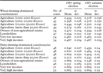
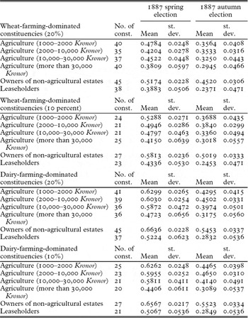
Descriptive statistics seem to show an association between farm size (respectively value) and agricultural specialisation, which can be detected in voting behaviour too. In order to see whether or not this relationship is driven by the problem of ecological inference, we select the 30 per cent of the constituencies where the output of wheat and the density of cows per hectare farmland were highest, and provide the average estimates for the share of votes for free trade for these districts only. Table 5 shows the results for the constituencies dominated by wheat and by dairy farming.
King's estimates for lambda/votes for free trade (30 per cent wheat- and 30 per cent dairy-farming-dominated constituencies only)

Just like the descriptive statistics, the analysis bears out our core hypothesis that wheat producers favoured protection much more strongly than dairy farmers. This was the case in both elections. In dairy districts, owners of very large estates and leaseholders were the only groups whose support for free trade fell under 60 per cent in the election in spring 1887. The contrast to the constituencies where wheat farming dominated could not be stronger. There, in spring 1887, support for free trade nowhere reached 50 per cent; even around 57 per cent of the smallholders whose farms had a value of 1,000 to 2,000 Kronor voted for protection. By autumn, the picture had changed slightly. The general tendency of voters from dairy districts to be more supportive of free trade than voters from wheat districts remained, but free-trade support diminished in both types of constituencies and among almost all groups of voters. The only group where it slightly increased were voters who had gained their right to participate in elections because they had a taxable income of about 800 Kronor per year, and who fell in the poorest category within this group.
4.5. Robustness
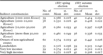
The results of King's algorithm perfectly fit the tendencies observed in the descriptive statistics and our expectations. Still, we will provide some robustness checks. First, it is possible to check whether the decline of the free trade vote between spring and autumn 1887 was due to manipulation rather than simply to dissatisfaction with the government. As for possible manipulations, our hypothesis is that these would most likely occur in constituencies where the elections were indirect, as here open voting was occasionally still practised. Accordingly, we select the indirect constituencies and provide the average estimates for these constituencies separately, expecting the smallholders’ vote for free trade to have been weaker here than in the mean of all Swedish constituencies (see Table 4). Table 6 shows the results.
King's estimates for lambda/votes for free trade (constituencies where voting was indirect)

Our estimates based on King's algorithm show that in actual fact the opposite was true. In indirect constituencies, the vote for free trade was in both elections stronger than average, i.e. when all Sweden is considered. If there was any electoral manipulation at all, it was clearly not associated with districts where voting was indirect and possibly not secret. This suggests that while, overall, free trade remained dominant in Swedish public opinion, the governmental party suffered the usual fate of incumbents and was punished by dissatisfied voters.
As indicated above, King's algorithm is the most advanced approach to solve the problem of ecological inference, but there is another, more traditional method that we can use for a robustness check. This method relies on ecological regressions, which were developed by Goodman (Goodman Reference Goodman1953) and are therefore also called ‘Goodman's regression’ (see above). The design is simple. Referring to Table 3, we know that:

This equation has the same form as a simple two variable ordinary least squares (OLS) regression equation such as

where Y is the dependent variable, which is similar to Vi, the constant a equals λJi, (1−xJi) is the independent variable, (λ−Ji−λJi) is the estimated coefficient for the independent variable and e is the error term. This method uses information from all constituencies together to produce estimates. The disadvantage is that it often produces impossible results, such as negative coefficients or coefficients above one, which implies that more than 100 per cent of votes were cast by members of a certain group of voters. Nevertheless, we apply this simple regression in order check the robustness of the results we obtained with the help of the more sophisticated method, King's algorithm.
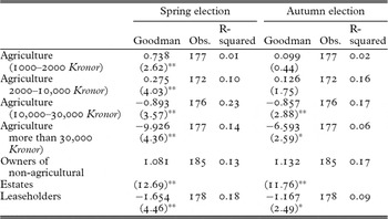
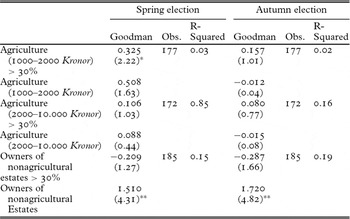
Table 7 provides the estimates for the constant, i.e. λJi. They show the same effects that already appear in the analysis above: smallholders seem to have voted for free trade (73.8 per cent), whereas large land owners (row 4) seem to have preferred protection. The weaknesses of Goodman's regression are apparent here. Some of the estimated coefficients show negative signs, which implies that a negative number of voters from this particular group voted for free trade. Although this is logically of course impossible, the direction of voting behaviour provides useful information. Table 4 also shows the estimated coefficients for the autumn election. The effects still appear, although much weaker. Smallholders seem to have lost much of their preference for free trade.
Goodman coefficients = the estimated constant a (simple OLS with robust standard errors)

Robust t statistics in parentheses
Each observation was weighted with the number of voters per constituency.
*significant at 5%; **significant at 1%
Note: The presented values are the estimates constant a in equation 5.
Table 8 provides the estimates for Goodman's regression, but now includes for some regressions a dummy for constituencies in which the numbers of voters from the particular group exceeded 30 per cent of the total electorate. The dummy for the category of farmers owning the smallest amount of land is positive (0.325) and significant: constituencies in which the number of voters who were smallholders exceeded 30 per cent voted significantly more strongly for free trade.
Goodman coefficients = the estimated constant a (simple OLS with robust standard errors), including dummy for concentrated areas

Robust t statistics in parentheses
*significant at 5%; **significant at 1%
Note: same estimation as in Table 4, but including a dummy which is equal to 1 if the number of voters owning estates of this particular value exceeds 30%.
Goodman's regression provides useful information, which generally supports our results derived with King's algorithm, although the coefficients themselves are not logically explainable.
A last robustness check focuses on the cut-off point for wheat- or dairy-dominated constituencies. We have shown above that in the 30 per cent of constituencies with the largest wheat output and the highest density of cows, voters preferred protection and free trade, respectively. Table 9 shows the results for the 10 and 20 per cent of constituencies with the largest output of wheat and highest density of cows. As one can see, the main result of our analysis – i.e. that voters in constituencies dominated by wheat production had a stronger interest in protection than voters of other constituencies, and that voters in constituencies where dairy farming was more common had a stronger interest in free trade – is not influenced by the choice of a different cut-off point.
Constituencies with 10 and 20 per cent highest wheat production and density of cows

5. Conclusion
In 1888, the Swedish government introduced tariffs for a number of agricultural and industrial goods. This policy change is frequently regarded as the outcome of a ‘quirk of fate’, to use Lewin's (Reference Lewin1988, p. 47) expression – i.e. of the tax scandal that cost the free-trade-supporting members for Stockholm their seats in parliament –, and in fact both elections returned free-trade majorities. In the present article, we ask which groups of voters voted for free trade, and examine whether their decisions match expectations that can be formed on the basis of trade models such as the specific factor models, that is, if voting behaviour can be considered rational.
In order to answer these questions, we first determine which groups of voters would have benefited from protectionism and which would have suffered. We do this on the basis of information on their income and on the amounts of land they owned or leased, and of data on farm sizes and the mix of agricultural outputs produced in the constituencies. These data allow us to determine that there was a close association between the size of the voters’ estates and their agricultural specialisation, with voters who owned or leased large estates producing import-competing commodities such as wheat. Smallholders, by contrast, focused on animal husbandry and were threatened by international competition to a much smaller degree or not at all.
In our analysis, we first apply a modern method from the political science literature, i.e. King's algorithm. We find that voters who did not own or lease land consistently favoured free trade. Agricultural voters, however, evidenced interesting variations between estate sizes. In the spring election, it was only the voters with the largest farms (that had a value of more than 30,000 Kronor) and leaseholders (who had to rent land with a value of at least 6,000 Kronor in order to be allowed to vote) whose support for free trade fell below 50 per cent. In the autumn election, by contrast, even 60 per cent of the smallholders voted for protection. However, protectionists gained support across the board, that is, not only among farmers who had voted for free-trade-supporting politicians in spring, but also among those who had predominantly favoured protection from the start. The fact that all groups of farmers, regardless of the value of landholding or the direction of specialisation, began to turn towards protection in autumn 1887 suggests that grievances or problems specific to individual sectors of agriculture – such as increasing exposure to competition from abroad – were not at the root of the change in voting behaviour. One obvious explanation is that this was mainly the effect of the backlash of public opinion against the incumbent party – a pattern that can be particularly often observed when elections follow each other closely. Another explanation could be that farmers, who due to their specialisation should have been opposed to protection, became unsure about whether they really benefited from free trade. This could have been caused by protectionist propaganda, which they might have believed due to a lack of experience, background knowledge or education. Objective information was probably costly to come by, and the turn towards protection could signal that smallholders fell prey to protectionist propaganda.
However, if we assume that voters were able rationally to choose the policy which makes them better off – this is what our analysis indicates – the slight move towards protection could indicate electoral manipulation. In order to exclude this possibility and to determine whether electoral manipulation or pressure exerted by owners of large estates on smallholders played a role – as it seems to have done in Germany a few years previously (Gerschenkron Reference Gerschenkron1943) –, we investigated constituencies where voting was indirect and occasionally still open separately. However, we found no evidence that this was the case: on the contrary, in indirect constituencies, free trade gained more support than average in both elections. The fact remains that in the course of the summer and early autumn 1887, small and middling farmers, erstwhile supporters of free trade, decided to vote against the governmental party in the second election of 1887.
The discussion above makes clear that research on voting behaviour based on aggregate data, even if analysed with sophisticated methods, still can only show a broad picture. This research needs the support of qualitative studies on a micro-level. However, especially in the context of economic history, where surveys and interviews of voters are not available, the above research is essential to gain insight into voters, voting decision and how policy was made.
Acknowledgements
For comments and helpful criticism thanks are due to Kevin O'Rourke, Kenneth Benoit, Jan Bohlin, Carsten Burhop, Kerstin Enflo, Sakari Heikkinen and Cheryl Schonhardt-Bailey, to the participants in the Baltic Sea Workshop in Helsinki in October 2009 and to two anonymous referees.