2. Methodology

Experimental campaigns were conducted at two separate institutions. (i) Flow visualisation tests were conducted at The University of Adelaide (Thebarton, South Australia) and (ii) TPIV tests were conducted at TUDelft (Delft, The Netherlands).

2.1. Structured porous coated cylinder

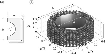
The SPCC used in this study has identical proportions to the original SPCC by Arcondoulis et al. (Reference Arcondoulis, Liu, Li, Yang and Wang2019). The SPCC design consists of a series of concentric interconnected C-shaped pieces, shown in figure 1(a). The dimensions $w$, $h$, $r$ and $l$ determine the SPCC overall PPI and porosity and the procedure of cloning and replicating C-chips into a full-span SPCC is discussed in detail in Arcondoulis et al. (Reference Arcondoulis, Liu, Li, Yang and Wang2019). A computer-aided design (CAD) representation created using ANSYS Workbench of an SPCC partial span is presented in figure 1(b). The inner diameter, $d$, and outer diameter, $D$, of the SPCC are related via $D = d + 2t$, where $t$ is the thickness of the porous layer. Since PCCs are typically compared by their ratio of thickness to inner diameter, $t/d$, it is convenient to express the inner diameter via

(2.1)\begin{equation} d = \frac{D}{1+2(t/d)}.\end{equation}

The porosity value, $\varPhi$ (%), of the SPCC is identical to that of previous SPCC studies (Arcondoulis et al. Reference Arcondoulis, Liu, Li, Yang and Wang2019, Reference Arcondoulis, Geyer and Liu2021a,Reference Arcondoulis, Geyer and Liub), being $\varPhi = 87$ %, calculated via $\varPhi = 100 \times (1 - V_{{SPCC}}/V_{{SC}})$, where $V_{{SPCC}}$ is the volume of the porous coating and $V_{{SC}}$ is the volume of a solid annulus with inner diameter $d$ and outer diameter $D$.

Figure 1.

A CAD representation of (a) the C-chip used to determine the SPCC PPI and porosity and (b) part of the SPCC span.

2.2. Flow visualisation experiments

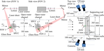
Tests were conducted to visualise the SPCC internal and near-wall flow fields prior to TPIV and to select suitable TPIV FOV locations (see figure 4). A schematic diagram of the water tunnel and experimental set-up is shown in figure 2. An SPCC with $D = 120$ mm, $t/d = 0.25$ and $2D$ span was 3-D printed using ultraviolet curing epoxy resin. The water tunnel was operated at a free-stream flow speed of $U_{0} = 0.06$ m s$^{-1}$, corresponding to an SPCC outer-diameter Reynolds number of $Re_{D} \approx 7 \times 10^{3}$. A controlling valve was used to slowly inject small parcels of concentrated blue food dye into the flow immediately upstream of the SPCC. Images were captured using a 24MP camera placed on the glass facing the cylinder. Photos with a short shutter speed of 1/1000 s were taken to observe instantaneous flow behaviour and were stacked over a 30 s period to estimate time-averaged flow fields. Photos were taken at three separate locations, focusing on the SPCC windward, mid-circumference and leeward regions, that were stitched together to obtain a full flow field of the lower half of the SPCC.

Figure 2.

Schematic diagram of The University of Adelaide water tunnel, used for flow visualisation within the SPCC internal porous layers.

By obtaining photos of specific cylinder regions, a clear line of sight can be obtained on a specific region of several pores. From these images, boundary layer profiles within the porous layer can be estimated from the concentration of red–green–blue (RGB) pixels, consistent with Liu et al. (Reference Liu, Hu, Lei and Nepf2018). The MATLAB Image Processing Toolbox was used to extract the concentrations of each RGB pixel (0–255). The dye is completely blue and treated as a reference value (i.e. $\bar {U}/U_{0} = 0$) and data are scaled by concentrations of red. An in-house code was developed to calculate velocity profiles that neglect erroneous data points (such as the structural members of the SPCC).

2.3. Particle image velocimetry experiments

The TPIV experiments were conducted in a low-speed water flume in the Department of Civil Engineering and Geosciences at TU Delft, The Netherlands. A schematic diagram of the TPIV set-up is presented in figure 3. The flume has a working section of 400 mm (wide) and a maximum working height of approximately 300 mm. The flume is inclined downward at 5$^\circ$ to produce a sufficient pressure differential to achieve a specified volumetric flow rate. A pressure-pump controlled the free-stream velocity at $U_{0} = 0.8$ m s$^{-1}$. The water temperature was recorded at 18$\,^\circ$C such that the kinematic viscosity was $\nu = 1.053 \times 10^{-6}\ \mathrm {m}^{2}\ \mathrm {s}^{-1}$. The SPCC parameters were $D = 96$ mm, $d = 64$ mm (as $t/d = 0.25$), achieved using $r = 1.8$ mm, $h = 5.4$ mm, $w = 2.8$ mm and $l = 1.6$ mm (see figure 1a). The SPCC was 3-D printed in one piece with a span of 385 mm (approximately $4D$) using a transparent ultraviolet curing epoxy resin. The outer-diameter Reynolds number is $Re_{D} = 7.3 \times 10^{4}$ which is comparable with the published data of PCCs (Sueki et al. Reference Sueki, Takaishi, Ikeda and Arai2010; Ruck et al. Reference Ruck, Klausmann and Wacker2011; Liu et al. Reference Liu, Wei and Qu2012; Naito & Fukagata Reference Naito and Fukagata2012; Geyer & Sarradj Reference Geyer and Sarradj2016). The difference in calculated Strouhal number between an SPCC and a bare cylinder shows little variation over $Re_{D} = 8 \times 10^4$ to $2 \times 10^5$ (Arcondoulis et al. Reference Arcondoulis, Liu, Li, Yang and Wang2019). This provides confirmation that the flow behaviour recorded during TPIV tests is indicative of higher-Reynolds-number flows associated with other PCC (and SPCC) aeroacoustic studies.

Figure 3.

Schematic diagram of the TPIV configuration.

The water in the tunnel was seeded with fine silt particles of mean diameter of 100 $\mathrm {\mu }$m that were illuminated by a Quantel EverGreen200 double-pulse Nd:YAG laser (532 nm wavelength, 200 mJ per pulse). One spherical and three cylindrical lenses were aligned to produce a 20 mm thick laser sheet. A mirror was used to reflect the laser sheet into the water as shown in figure 3. Four LaVision Imagers (sCMOS: 4MPx, 7.4 $\mathrm {\mu }$m pixel pitch) were equipped with 105 mm Nikon Micro-Nikkor prime lenses and Scheimpflug adapters were used to align the focal plane with the laser sheet (perpendicular to the water tunnel glass walls).

Synchronisation of the laser pulses and image acquisition was accomplished using a LaVision programmable timing unit in combination with the LaVision DaVis 8.4 software package. Images were acquired at 15 Hz which is approximately 10 times the expected vortex shedding frequency of the SPCC (based on the SPCC exhibiting a vortex shedding Strouhal number of $St \approx 0.19$ to 0.2 (Norberg Reference Norberg2003; Arcondoulis et al. Reference Arcondoulis, Geyer and Liu2021b) and therefore a vortex shedding frequency of $f \approx 1.6$ Hz). The standard MART algorithm with 10 iterations and 9 intermediate Gaussian smoothing stages was carried out for the volume reconstruction of the TPIV data (Elsinga et al. Reference Elsinga, Scarano, Wieneke and van Oudheusden2006). All velocity vectors had ${\rm SNR} \geq 2$ above the mean velocity which is within normal parameters (Elsinga et al. Reference Elsinga, Scarano, Wieneke and van Oudheusden2006; Scharnowski & Kähler Reference Scharnowski and Kähler2020). Each interrogation window had dimension $96 \times 96 \times 96$ voxels which included on average between 6 and 10 particles, constituting a slightly lower but appropriate seeding concentration according to Scarano (Reference Scarano2012). The authors adopted a relatively low particle density (${\rm ppp} < 0.10$) compared with what modern TPIV can cope with, because the low-speed sequence was processed with the FastMART algorithm which was proven for this case to yield better results for TPIV (Elsinga et al. Reference Elsinga, Scarano, Wieneke and van Oudheusden2006). The 3-D vector calculations were conducted using a conventional multi-pass direct correlation algorithm (Scarano Reference Scarano2001) (from 128 to 96 with 2 passes per iteration). Image correlation was carried out with a multi-pass algorithm with a final FOV size (see figure 4) and 75 % overlap. Table 1 summarises the TPIV parameters. Calibration of the FOV and self-calibration for the alignment of the imaged volume with the illuminated one were conducted using a Type-7 calibration plate, placed at three spanwise planes with the same $xy$ coordinates in the spanwise-centre of the laser sheet and at the laser sheet edges (i.e. $z = -10$, 0 and 10 mm). The tunnel was filled with water (at zero velocity) to ensure that any refraction effects between water and air were factored into the calibration. The LaVision DaVis 8.4 software package was used to carry out the calibration.

Figure 4.

The FOVs 1 and 2. Lines within each FOV are referred to as $\theta$-lines used during post-processing. Image is to scale.

Table 1.

Summary of TPIV parameters.

The SPCC was placed approximately $x = 6$ m downstream of the flume entrance. Assuming that the flow develops a laminar (Blasius) boundary layer, the boundary layer height can be estimated via $\delta (x) = 5\sqrt {x\nu /U_{0}} \approx 14$ mm. The SPCC is placed at height much greater than 14 mm (see figure 3). The turbulence intensity of the flow at the SPCC streamwise location is $\sigma _{u} = u'/U_{0}$, calculated to be approximately 3 %. The uncertainty in the mean velocity field is calculated as $\epsilon _{u} = \sigma _{u}/\sqrt {N} \approx 10^{-3}$, where $N$ is the number of TPIV temporal samples. Similarly, the uncertainty in the streamwise velocity fluctuations is $\epsilon _{u'} = \sigma _{u}/\sqrt {2(N-1)} \approx 6.7 \times 10^{-3}$. These values are well within the uncertainty values quoted for a similar scale TPIV investigation of a wall-mounted short cylinder in water conducted by Zhu et al. (Reference Zhu, Wang, Wang and Wang2017).

Figure 4 presents the specific locations of the TPIV FOVs. The position of FOV 1 is chosen to investigate the interaction between the free-stream flow and the porous layer on the windward region, and how the porous layers affect the region around the stagnation point, and the position of FOV 2 is chosen to quantify the internal flow field and the development of the inner-diameter boundary layer. Along the $r/t$-line streamwise and vertical velocity components are calculated to understand the deceleration of the flow into the porous layer. Flow quantities are extracted from lines drawn through FOV 2, herein referred to as $\theta$-lines. The reconstructed flow field in FOV 1 has $93 \times 71 \times 59$ pixels and in FOV 2 has $115 \times 97 \times 51$ pixels, with a spatial resolution of 0.278 mm. The SPCC used for the TPIV experiments has elliptical pores with minor and major axis radii of 3.5 and 5 mm, respectively, and structural member thickness of approximately 1.2 mm. Therefore the FOV spatial resolution is adequate to capture local flow behaviour around and within the pore structures.

3. Flow visualisation

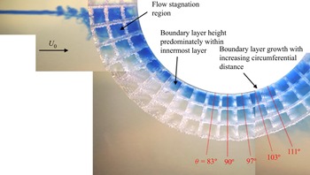
The result presented in figure 5 reveals for the first time an experimentally obtained internal flow field of an SPCC. The flow is directed from left to right and as the dye approaches the cylinder outer surface, the change in dye concentration indicates a transition from a laminar to a turbulent flow. The dye-stained flow proceeds to enter the porous structure and accumulates at the most-windward region (representing flow stagnation). The dye continues to flow around the cylinder and through the porous layers, remaining attached to the inner diameter (as seen by dye accumulation) representing boundary layer development that is confined to the innermost porous layer. Further downstream the boundary layer develops, separates into a shear layer within the porous layers and eventually bleeds into the free-stream flow region. Quantification of time-averaged boundary layer profiles from these data is provided in § 5 and is compared with TPIV results.

Figure 5.

Flow visualisation result at $Re \approx 7 \times 10^{3}$. Images are stitched together to improve the line of sight of each region.

4. Windward region

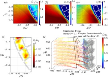
The total velocity is defined here as $U = [u,v,w]$, an overline represents time averaging and the $|_{z}$ notation denotes averaging over the spanwise direction ($z$ direction). An overview of the flow field at the windward region is presented in figure 6. Flow acceleration around the SPCC outer diameter is observed in figure 6(a–c) in the region $x/D = -0.5$ to $-0.4$ and $y/D = -0.35$ to $-0.25$, which is commonly observed around smooth cylindrical bodies. The flow within the porous layer is nearly stagnated. In figure 6(a), $|\bar {U}|_{z}/U_{0} \approx 0$ within the porous layer corresponds to the locations of the SPCC structural members. Note that at some structural member locations $|\bar {U}|_{z}/U_{0} \neq 0$ due to the averaging of velocities over the $z$ planes. This is explained by the presence of spanwise flow and reverse flow. 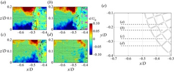Flow in the negative $x$ direction, presented in figure 6(d), is observed in the outermost porous layer. The local minima of these reverse-flow regions correspond to the intersection of circumferential and radial pore struts, as fluid travels through and around pore members in the spanwise direction. The flow at the near-wall region is depicted by 3-D streamlines in figure 6(e). The free-stream flow is accelerated around the SPCC outer diameter and diverges in the spanwise direction, about $z/D = 0.1$. The spanwise flow component $\bar {w}/U_{0}$ at the near wall and within the porous layers at various $xz$ planes is further investigated and presented in figure 7.

Figure 6.

Time-averaged velocity components recorded in FOV 1: (a) $|\bar {U}|_{z}/U_{0}$, (b) $\bar {u}|_{z}/U_{0}$, (c) $\bar {v}|_{z}/U_{0}$, (d) $\bar {U}|_{z}/U_{0} < 0$ and (e) streamlines of $\bar {U}/U_{0}$. Flow is from left to right.

Figure 7.

Time-averaged spanwise velocity component $\bar {w}/U_{0}$ superimposed with streamlines recorded at (a) $y/D = -0.18$, (b) $y/D = -0.22$, (c) $y/D = -0.28$ and (d) $y/D = -0.33$ as identified in (e) $xy$-plane view of the SPCC in FOV 1. Slices of the SPCC in (a–d) are shaded in pink. Flow is from left to right.

Figure 7 presents four $xz$ planes at different $y/D$ stations (with decreasing $y$ values). At each $xz$ plane the free-stream flow is seen to diverge as it approaches the SPCC outer diameter, as observed by the near-equal and opposite spanwise flow fields about $z/D = 0.1$ (corresponding to the midspan of the SPCC). In the absence of flow field data over a longer portion of the span, it is difficult to determine whether this divergence pattern (centred about $z/D = 0.1$ in this case) is periodic along the span, or whether it only occurs at the midspan of the SPCC. The streamlines in all planes show that the free-stream flow penetrates the outermost porous layer and then stagnates. Scattered areas of $|\bar {w}|/U_{0} = 0.05$ are seen in the outermost porous layer that are due to local interactions with porous members and the merging of the external and internal flow fields. The spanwise velocity amplitude is observed to decrease with increasing distance away from $y/D = 0$, to $|\bar {w}|/U_{0} = \pm 0.05$, as measurements are obtained further from the stagnation region of the SPCC. Weaker divergence at the outer diameter is expected further from the stagnation region where the flow field is dominated by $u$ and $v$ ($(|\bar {u}|_{z}|/U_{0})_{{max}} \approx 0.4$ and $(|\bar {v}|_{z}|/U_{0})_{{max}} \approx 0.4$).

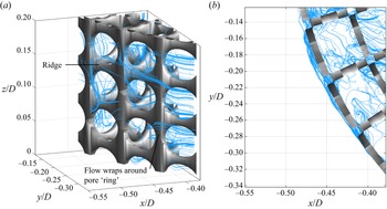
Streamlines originating near the porous surface are calculated in FOV 1 using an in-house MATLAB code. A CAD model of the SPCC is imported and its coordinates are extracted and matched to the nearest point in the 3-D flow field volume. These flow field points are typically within 1 mm from the porous surface (recall the TPIV spatial resolution is 0.278 mm) and are used as the starting points for streamlines. These streamlines always originate from valid coordinates within the FOV and avoid any interpolation between streamline starting points and FOV data points. Figure 8 presents near-wall and internal streamlines of $\bar {U}$ within FOV 1. Regions of highly localised vortical structures and chaotic flow patterns in the pore regions near the structural members are observed, where flow is seen to wrap around the structural members. In figure 8(a) some streamlines are seen to follow the outer diameter of the SPCC, along a ridge of solid material (e.g. along $z/D \approx 0.15$). In the absence of a ridge, the flow wraps around the ring of the pore penetrating the outermost porous layer, leading to local regions of vorticity around the porous outer layer, which is also seen in figure 8(b).

Figure 8.

Streamlines at the windward outer diameter and within the porous layers. (a) Arbitrary 3-D view and (b) spanwise ($z$ direction) view. Flow is in the positive $x$ direction.

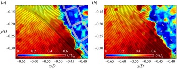
Instantaneous (and simultaneous) $U/U_{0}$ flow fields investigated at a closed-pore plane and an open-pore plane are presented in figures 9(a) and 9(b), respectively. In the closed-pore slice the flow is not seen to penetrate the outermost porous layer and the stagnated flow region within the porous layers has a defined circular-shaped boundary immediately outside of the SPCC outer diameter. The open-pore slice has a less clear circular boundary as observed near $x/D = -0.5$ and $y/D = -0.18$. Streamlines are observed to enter the porous layers and pass around some structural members at the open-pore plane, yet not at the closed-pore plane.

Figure 9.

Instantaneous snapshots of $U/U_{0}$ recorded at (a) a closed pore ($z/D = 0.07$) and (b) an open pore ($z/D = 0.1$). The open- and closed-pore flow fields are obtained simultaneously. Flow is from left to right.

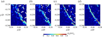
In figure 10 values of $|\bar {\omega }_{z}|D/U_{0}$ are plotted on $xy$ planes with the corresponding SPCC slice. There are regions of strong vorticity near the porous structural members as the flow attempts to both enter the porous region and also pass by the outer diameter resulting in strong shear. The flow needs to rotate about a pore ridge in order to enter the porous layer (shown in figure 8) that corresponds to small localised regions of high vorticity. This explains why the peak vorticity values are greater at lower $y/D$ values, as the flow speed is higher there and has a narrower line of sight to enter the structure, due to the angle of the porous layer relative to the $y$ axis, thus leading to a greater intensity of flow rotation (and thus vorticity). In conjunction with this flow rotation, vortical structures in the flow propagate towards the SPCC via pressure gradients and accumulate at the solid sections of the SPCC outer diameter. These mechanisms, which yield regions of concentrated localised vorticity, therefore explain why at different $z/D$ slices the location and magnitude of peak vorticity are seen to change. In figure 10(a) the $z/D$ plane corresponds to a plane that passes through the centre of a pore, and the planes of figures 10(b) to 10(d) shift in the $z$ direction towards a structural member (edge of a pore) that restricts incoming flow. This explains why at a particular $z/D$ plane the flow is observed to enter a pore without obstruction, yet at the same $xy$ coordinate but with a different $z/D$ plane, this point corresponds to a porous structural member, and hence a significant increase in the $z$ component of vorticity is observed.

Figure 10.

Contours of $|\bar{\omega}_{z}|D/U_{0}$ recorded on $xy$ planes in FOV 1 and the corresponding SPCC section slice, obtained at (a) $z/D = 0$, (b) $z/D = 0.04$, (c) $z/D = 0.1$ and (d) $z/D = 0.16$. Flow is in the positive $x$ direction.

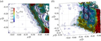
The chaotic flow field at the near wall and within the porous layer is visualised using turbulent kinetic energy (TKE), $k_{xyz}$ (%), calculated in FOV 1 via $k_{xyz} = 100 \times (1/2)(\overline {u^{'2}} + \overline {v^{'2}} + \overline {w^{'2}})/U_{0}^{2}$. The TKE is presented in figure 11, where it is observed that within the porous layers the TKE is seen to be constant, $k_{xyz} \approx 1.5$ %, yet near the outer diameter there exists a region of $k_{xyz} \approx 2$–2.5 %. The complex interaction between the geometry of the outer layer and incoming flow field leads to a local increase of TKE; yet the internal flow field, immediately aft of this layer, shows much weaker TKE. This reveals that the outermost porous layer acts as the main transition between the external and internal flow fields. Near $x/D = -0.4$ and $y/D = -0.3$ a local region of $k_{xyz} = 3$ % is observed. This increased TKE relative to the TKE observed near the outer diameter at smaller $\theta$ values is due to the local acceleration of the flow around the cylinder outer diameter and its interaction with the outer porous layer.

Figure 11.

Turbulent kinetic energy, $k_{xyz}$ (%), in FOV 1 presented in (a) $xy$-plane view and (b) arbitrary 3-D view. Flow is in the positive $x$ direction.

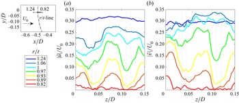
To further investigate how the free-stream flow penetrates the porous layer, values of $\bar {u}/U_{0}$ and $\bar {v}/U_{0}$ were recorded along the $r/t$ line. For convenience, the $x$ coordinate here is replaced with an $r/t$ coordinate, where $r$ is a radial distance that represents the distance from the SPCC inner diameter and $t$ is the thickness of the porous layer such that $r/t = 0$ denotes the inner cylinder diameter $d$ (corresponding to $x/D = -0.3125$) and $r/t = 1$ represents the outer diameter $D$ (i.e. $r/t = 1$ is at $x/D = -0.5$). The $r/t$ line follows an open-pore path, so that along the $z$ axis, local minima and maxima corresponding to the flow interacting with a structural member or flowing into the porous layer, respectively, can be observed. Figure 12 presents the variation of $|\bar {u}|/U_{0}$ and $|\bar {v}|/U_{0}$ in the $z$ direction as the flow approaches the outer windward surface of the SPCC and within the porous layer. This figure clearly shows deceleration twice: gradual flow deceleration towards the outer porous layer and rapid deceleration once the flow enters the porous layer, where the narrow region between the grey dashed lines represents the structural member of the pore. At $r/t = 1.24$, $|\bar {u}|/U_{0}$ shows little variation in $z/D$, as the flow approaching the windward surface of the SPCC has not interacted with the porous surface. However, at $r/t = 1.06$, significant variation in $|\bar {u}|/U_{0}$ with respect to $z/D$ is observed, and this variation is seen to increase with decreasing $r/t$. In other words, the streamwise velocity component is affected by the porous structure; at the structural member, it stagnates, and at the open pores, it flows into the porous layer. Further inside the porous layer, at $r/t = 0.82$, the flow has nearly stagnated at all $z/D$ locations. The stagnation of the streamwise velocity occurs rapidly between $r/t = 0.82$ and 0.89. At values of $r/t < 0.82$ the streamwise velocity is totally stagnated. Similar behaviour is noticed for $|\bar {v}|/U_{0}$, where stagnation occurs between $r/t = 0.82$ and 0.89 and the first noticeable local influence of the porous structure on the oncoming flow field takes place at $r/t = 1.06$.

Figure 12.

Variation of the flow field along $z/D$ (spanwise direction), approaching and entering the windward side of the SPCC between $z/D = 0$ and 0.15: (a) $|\bar {u}|/U_{0}$ and (b) $|\bar {v}|/U_{0}$. Each line is represented by an $r/t$ coordinate denoted in the top-left schematic diagram and the narrow area between the grey dashed lines represents the pore structural members.

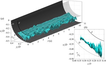
The boundary of the stagnation region was investigated both temporally and spatially, i.e. the most-upstream coordinates ($x,y$) were located that satisfy $u(x,y,t)|_{z} = 0$ in FOV 1 at each time step. The use of spanwise averaging and detection of stagnation using the streamwise velocity is assumed to provide an accurate estimate of the stagnation boundary of the SPCC. Figure 13 presents the calculated stagnation boundary, varying in time and $xy$ space. Flow further from the $y/D = 0$ axis is more temporally stable whereas flow closer to the stagnation region, $y/D \approx 0$, shows significant fluctuations in time. The stagnation region in the windward porous layers is subject to large-scale low-frequency oscillations. The stagnation region is always within the SPCC outer diameter and encroaches periodically within approximately 90 % of the porous layer thickness. The influence of the oscillatory behaviour on the windward region results in a pressure shift further around the SPCC inner-diameter circumference and contributes to the boundary layer development from the SPCC inner diameter: internal flow field boundary layers are discussed in § 5.

Figure 13.

Temporal–spatial diagram of the streamwise flow stagnation in FOV 1, defined as $u(x,y,t)|_{z} = 0$, over an arbitrary time period, $t = 1$ to 11 s. Images are presented in (a) isometric view and (b) $xy$ plane facing $t = 1$ s. Flow is in the positive $x$ direction.

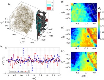
A cross-correlation study was conducted to further understand the relationship between the external flow field with the near wall and internal flow field at the windward side of the SPCC. The normalised cross-correlation of $U$ in FOV 1, $R_{ij}$, between a single reference point ($i$) and all other points in the FOV ($\,j$) was calculated via

(4.1)\begin{equation} R_{ij}(\tau) = \frac{1}{\sqrt{\langle U^{2}_{i,t}\rangle \langle U^{2}_{j,t}\rangle}} \frac{1}{N_{\tau}}\sum^{N_{\tau}}_{n_{\tau} = 1}(U_{i,t_{n_{\tau}}}U_{j,t_{n_{\tau}}+\tau}),\end{equation}

where $n_{\tau }$ is a temporal index ($n_{\tau } = 1:N_{\tau }$) and $\tau$ (s) is a temporal shift. Three reference points were selected to help understand the influence of the external flow field on the fluid region within the porous layer, as presented in figure 14. The reference point $i_{1}$ is located in the top-left corner of FOV 1 (external flow field), $i_{2}$ is placed along $r/t = 1$ within an open-pore region and $i_{3}$ is located also in an open-pore region further into the porous layers (top-right of FOV 1). In figure 14(a) iso-surfaces of $R_{ij} \geq 0.9$ for reference locations $i_{1}$, $i_{2}$ and $i_{3}$ are shown. Clearly, using reference location $i_{1}$ it is seen that the external flow field correlation region does not extend into the porous layer. This reveals that the temporal behaviour of the external flow field is uncorrelated with the internal and near-wall flow fields. Using reference locations $i_{2}$ and $i_{3}$ it is shown that the flow along the SPCC outer diameter is strongly correlated, which is supported by the observation of streamlines along the porous outer-diameter ridges (in figure 8). Some strong correlation is also observed between the flow field at $r/t = 1$ and the near-wall region centred about $x/D = -0.5$ and $y/D = -0.25$ showing that the interaction of the shear flow as it passes the SPCC outer diameter is strongly correlated with the local vortical regions in the outermost porous layer. Using $i_{3}$ as a reference location also reveals that there is a strong correlation between the inner region and outer regions of the external flow fields, which is an interesting result. The complex streamline patterns of the internal flow field shown in figure 8 appear to be highly chaotic yet there is indeed a temporal and spatial relationship between the flow fields of each porous layer. Figure 14(e) presents values of $u'(t)/U_{0}$, recorded at $i_{1}$, $i_{2}$ and $i_{3}$. From these data, point $i_{1}$ possesses the weakest velocity fluctuations (as expected) and points $i_{2}$ and $i_{3}$ possess strong fluctuations with maxima at $|u'(t)|/U_{0} \approx 0.5$ and 0.3, respectively. By comparison of the $i_{2}$ and $i_{3}$ time series, there does not appear to exist any clear trend or temporal offset between the signals. It can be therefore inferred that any strong fluctuations recorded at $i_{2}$ do not convect downstream to $i_{3}$ and the velocity fluctuations at these two points are driven by uncorrelated mechanisms.

Figure 14.

Cross-correlation, $R_{ij}$, of $U(x,y,z,t)$ in FOV 1. Locations $i$ denote fixed reference locations in the $xy$ plane ($z/D = 0.08$). (a) Iso-surfaces of $R_{ij} \geq 0.9$ for three reference locations $i_{1}$, $i_{2}$ and $i_{3}$, and values of $R_{ij}$ recorded in the $xy$ plane ($z/D = 0.08$) of (b) $i_{1}$, (c) $i_{2}$ and (d) $i_{3}$. Flow is in the positive $x$ direction. (e) Normalised time series of fluctuating streamwise velocity component, $u'(t)/U_{0}$, recorded at $i_{1}$, $i_{2}$ and $i_{3}$.

5. Mid-circumference region

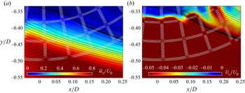
Time-averaged velocity fields at the near wall and within the porous layer for FOV 2, averaged in the $z$ direction, are presented in figure 15. Only the $\bar {u}|_{z}/U_{0}$ and $\bar {v}|_{z}/U_{0}$ flow components are presented here (for brevity) as the flow field is dominated by the streamwise flow component. Values of $\bar {u}|_{z}/U_{0}$ are presented in figure 15(a). Near the inner diameter $\bar {u}|_{z}/U_{0}$ is considerably lower than near the SPCC outer diameter and the low-velocity region expands with increasing streamwise distance, which is clear evidence of boundary layer growth on the inner diameter. The boundary layer then grows, separates into a shear layer and passes through the porous layer and beyond the outer diameter. Values of $\bar {v}|_{z}/U_{0}$ (figure 15b) increase with $\bar {u}|_{z}/U_{0}$ in both increasing radial and $x$ distance. Note that $\bar {v}|_{z}/U_{0}$ is presented with a colourbar limit smaller than $\bar {u}|_{z}/U_{0}$ to permit the visualisation of flow structures near the inner diameter. This helps reveal time-averaged velocity fluctuations that are related to the onset of instabilities that originate from the inner diameter and travel through the porous layers. As observed from the streamline pattern, the flow near the inner diameter at $x/D \approx 0$ travels in the streamwise direction, and as the shear layer develops, increased radial flow component is observed and, further downstream, the internal flow field interacts with the accelerated flow region in the outermost porous layers and gains velocity in the streamwise direction.

Figure 15.

Time-averaged velocity components recorded in FOV 2 averaged over the spanwise direction superimposed with streamlines (a) $\bar {u}|_{z}/U_{0}$ and (b) $\bar {v}|_{z}/U_{0}$. A CAD file is overlaid onto the contour plot to represent the SPCC. Flow is from left to right.

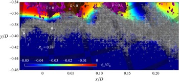
From the $\bar {u}|_{z}/U_{0}$ and $\bar {v}|_{z}/U_{0}$ flow fields presented in figure 15 it is difficult to determine whether any reverse flow occurs with the boundary layer. Figure 16 identifies regions of reverse flow (denoted by $\bar {u}<0$ and $\bar {v}>0$) and a region of constant correlation from a reference point $i$. These data are calculated in three dimensions but only the $xy$-plane projection is presented for clarity. Values of $\bar {v}|_{z}/U_{0}$ (figure 15b) are included for reference. At $x/D \approx 0$ and $y/D > -0.34$ flow is observed to travel towards the inner diameter ($\bar {v}>0$) and then immediately downstream at $x/D \approx 0.05$ the flow is seen to travel in the opposite direction to the free stream ($\bar {u}<0$). This represents some weak anticlockwise flow rotation with structures of length 0.05$D$ centred about $x/D \approx 0.02$ and $y/D \approx -0.33$. Further downstream at $x/D \approx 0.12$ the flow again travels back towards the inner diameter, yet further visualisation of within the boundary layer here is not possible due to the distance of the upper limit of the FOV to the inner diameter. The key observation is that the reverse-flow regions exist near the inner diameter and that the edge of the shear layer (where $\bar {v}|_{z}/U_{0} < -0.05$) very closely resembles the pattern of constant correlation ($R_{ij} = 0.88$). Regions of $R_{ij} > 0.88$ (not shown) exist further from the inner diameter. This correlation value was chosen to reveal coherent structures within the porous layer and that the edge of the stagnation region closely resembles the cross-correlation interface to the shear layer within the porous media. To help understand how the boundary layer develops with radial and circumferential distance, quantifications of the velocity profiles within the porous layers are presented in figure 17.

Figure 16.

Cross-correlation, $R_{ij} = 0.88$, of $U(x,y,z,t)$ in FOV 2 (shaded grey), where location $i$ denotes a fixed reference location in the $xy$ plane ($z/D = 0.08$). Values of $\bar {v}|_{z}/U_{0}$ (figure 15b) are included for reference and regions of reverse flow, $\bar {u}<0$ and $\bar {v}<0$, are shaded in maroon and purple, respectively. Flow is in the positive $x$ direction.

Figure 17.

Profiles of flow components recorded along FOV 2 $\theta$-lines, shown in figure 4: (a) $\bar {u}|_{z}/U_{0}$, (b) $\bar {v}|_{z}/U_{0}$, (c) $\bar {U}_{\theta }|_{z}/U_{0}$ and (d) $\bar {U}/U_{0}$ estimated from flow visualisation data in § 3. A vertical dotted line is drawn along $r/t = 1$ to denote the outer diameter of the SPCC.

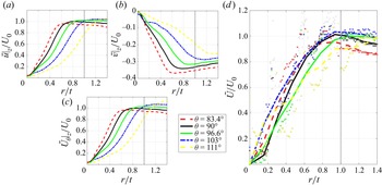
The $\bar {u}|_{z}/U_{0}$ and $\bar {v}|_{z}/U_{0}$ profiles are presented in figures 17(a) and 17(b), respectively, to further investigate boundary layer development within the porous layer. Note that within the porous layers of FOV 2 there exists little spanwise variation and therefore the spanwise-averaged results are indicative of the velocity profiles at any $z/D$ station. The time-averaged tangential velocity component, $\bar {U}_{\theta }|_{z}/U_{0}$, presented in figure 17(c) is used to estimate boundary layer thickness values. Profiles of $\bar {u}|_{z}/U_{0}$ reveal that the boundary layer grows with increasing circumferential distance, as shown in figure 15. The velocity profiles of $\bar {u}|_{z}/U_{0}$ and $\bar {U}_{\theta }|_{z}/U_{0}$ (figure 17c) bear much similarity due to the streamwise flow component dominating the internal flow field. The $\bar {v}|_{z}/U_{0}$ profiles reveal that for each $\theta$-line the normal flow component measured from within the porous layer to beyond the SPCC outer diameter increases rapidly, consistent with numerical simulations (Naito & Fukagata Reference Naito and Fukagata2012).

In the absence of a larger FOV that captures the asymptotic value of the boundary layer, the 99 % boundary layer thickness for each $\theta$-line is estimated using $0.99\bar {U}_{\theta }(r/t = 1.4)|_{z}/U_{0}$. The boundary layer thickness $\delta _{99}$ for a given $\theta$-line is labelled $\delta |_{\theta }$ and normalised with inner diameter, $d$. By inspection of $\bar {U}_{\theta }|_{z}/U_{0}$ in figure 17(c), $\delta |_{83.4^{\circ }} = 0.14d$, $\delta |_{90^{\circ }} = 0.18d$, $\delta |_{96.6^{\circ }} = 0.21d$, $\delta |_{103^{\circ }} = 0.28d$ and $\delta |_{111^{\circ }}$ extend beyond $r/t = 1.4$. It should be mentioned that from these results there is no evidence of boundary layer development on the SPCC outer diameter.

The extraction of time-averaged velocity $\bar {U}/U_{0}$ from the flow visualisation experiment is presented in figure 17(d). A third-order polynomial is fitted to the shaded data points only, neglecting the open data points. The open data points are distinguished from the shaded data points by an in-house code that detects the SPCC structural member RGB concentrations (that are typically white). The $\bar {U}/U_{0}$ values show some agreement with $\bar {u}|_{z}/U_{0}$ albeit the flow visualisation data were obtained at one-tenth the Reynolds number of the TPIV experiments. These results provide further validation of the existence of a boundary layer developing over the SPCC inner diameter over a Reynolds number range spanning an order of magnitude.

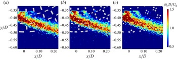
Contours of $|\bar{\omega}_{z}|D/U_{0}$ in FOV 2 are presented in figure 18 revealing a strong shear layer with high vorticity, for all $xy$ planes presented. The strongest region of vorticity occurs at the most-upstream region of FOV 2, where the kinetic energy of the shear layer is greatest, prior to its energy being distributed within the porous layer via chaotic interactions with porous members. This region of peak vorticity in figure 18 is coincident with where the boundary layer profiles posses their greatest slope (i.e. $(\mathrm {d}\bar{U}_{\theta }|_{z}/U_{0})/\mathrm {d}r \gg 0$ in figure 17c). The greatest vorticity is observed closest to $\theta = 90^{\circ }$, where values of $\bar {u}|_{z}/U_{0} \approx 1$ within the porous layer, thereby causing interaction with the porous structural members and generating vortices. At larger values of $\theta$, $\bar {u}|_{z}/U_{0} \approx 1$ occurs further from the porous layer and therefore does not produce the same vorticity due to the lack of interaction with the porous structure. Further visualisation of the development of vorticity within the shear layer is presented in figure 19(a). The width of the vorticity band in terms of $r/t$ is seen to increase with $\theta$ values. The widening of this band, in addition to its decrease in amplitude ($|\bar{\omega}_{z}|_{{max}}D/U_{0} \propto 1/\theta$), is consistent with a shear layer or jet that widens and becomes less rotational with increasing distance downstream.

Figure 18.

Contours of $|\bar{\omega}_{z}|D/U_{0}$ recorded on $xy$ planes in FOV 2 and the corresponding SPCC section slice, obtained at (a) $z/D = 0$, (b) $z/D = 0.02$ and (c) $z/D = 0.04$. Flow is in the positive $x$ direction.

Figure 19.

Profiles of flow components recorded along FOV 2 $\theta$-lines, shown in figure 4: (a) $|\bar {\omega }_{z}|_{z}D/U_{0}$ and (b) $k_{xyz}|_{z}$ (%). A vertical dotted line is drawn at $r/t = 1$ to denote the outer diameter of the SPCC.

The distribution of $k_{xyz}|_{z}$ relative to $r/t$ (figure 19b) exhibits a similar profile to the boundary layers in figure 17(c). The values of $k_{xyz}|_{z,{max}}$ occur near the SPCC outer diameter and the near-wall region and TKE amplitudes diminish with increasing downstream distance within the porous layers and beyond the SPCC outer diameter. Beyond the shear layer in the radial direction, turbulent structures exist throughout the flow and are independent of their position within or outside the porous layers. The peak TKE values are typically within 5 %. The $k_{xyz}|_{{max}}$ values recorded in the near-wall region for $r/t \geq 1$ are comparable with those of another SPCC wind tunnel test (Arcondoulis et al. Reference Arcondoulis, Geyer and Liu2021b) where at $x/D = 0.75$, $k_{x}|_{{max}} \approx 3$% where $k_{x} = 100 \times (1/2)(u^{'2}/U_{0}^{2})$ (%) was obtained via hot-wire anemometry. The assumption that the $k_{x}$ and $k_{xyz}$ values should be similar at this SPCC location is justified due the dominant component of velocity in FOV 2 being in the $x$ direction.

Proper orthogonal decomposition (POD) was performed to elucidate the development of the shear layer within the porous layers and the vortex shedding mechanism of the SPCC. Here POD was conducted on $u'(x,y,t)$ for each $xy$ plane. The vertical fluctuating velocity component is not considered here, as $|u'| \gg |v'|$ and has little contribution to the total fluctuating velocity in the shear layer within the porous media. 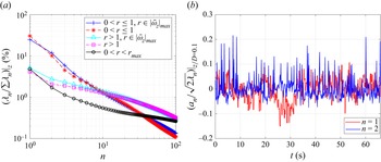Eigenvalues, $\lambda _{n}/\sum \lambda _{n}$ (%), presented in figure 20(a) are averaged over the $z$ direction (for brevity). Eigenvalues are calculated in five different regions of FOV 2, classified using a radial distance, $r$, such that $r = 0$ at the inner diameter and $r = 1$ at the outer diameter. Eigenvalues calculated within the porous layers are denoted as $0 < r \leq 1$, eigenvalues calculated within the porous layers but only within the region of the shear layer (as determined by $|\bar{\omega}_{z}|D/U_{0} >1$; see figure 18) are denoted $0 < r \leq 1$, $r \in |\bar {\omega }_{z}|_{{max}}$, eigenvalues outside the porous layers are denoted $r > 1$, eigenvalues calculated outside the porous layers but only within the region of the shear layer (as determined by $|\bar {\omega }_{z}|D/U_{0} >1$) are denoted $r > 1$, $r \in |\bar {\omega }_{z}|_{{max}}$ and eigenvalues calculated within the entirety of FOV 2 are denoted $0 < r < r_{{max}}$, where $r_{{max}}$ represents the boundaries of FOV 2. From figure 20(a) the strongest lower-order modes are observed within the porous layers. The higher-order modes within the porous layers are weaker than outside the porous layers, which is consistent with the distribution of TKE (see figure 19b) where stronger TKE is recorded outside the porous layers. Eigenvalues within the shear layer are similar to those recorded within the porous layers (that also includes the shear layer), revealing the shear layer flow is responsible for the low-order modes. This is supported by the lower-order modes outside the porous layers being much weaker than inside the porous layers.

Figure 20.

(a) Plots of POD eigenvalues, $(\lambda _{n}/\sum \lambda _{n})|_{z}$ (%), calculated on $u'(x,y,t)$ in different regions of FOV 2 and (b) time series of the temporal mode coefficients, $a_{n}$, normalised by the corresponding eigenmode, $\lambda _{n}$, for $n = 1$ and 2, calculated at $z/D = 0.1$.

The time series of the POD temporal mode coefficients, $a_{n}$, within $0 < r \leq 1$, $r \in |\bar {\omega }_{z}|_{{max}}$ were calculated and are presented in figure 20(b). An indicative $xy$ plane ($z/D = 0.1$) was chosen for figure 20(b) to reveal the strongest contribution of the second mode, $n = 2$ (in an open pore). The first mode, $n = 1$, reveals long-time-scale cycles, suggesting that this is possibly an entry–exit flow behaviour linked to entrainment of fluid within the porous layer (Naito & Fukagata Reference Naito and Fukagata2012). Note that the amplitudes of $n = 1$ are typically less than $n = 2$; this is not the case at other $z/D$ planes, yet the period of the $n = 1$ temporal mode coefficients at other $z/D$ planes is significantly lower than any feasible vortex shedding period and thus $n=1$ is not further considered here. At $n = 2$ a strong series of spikes in the time series are observed and via fast Fourier transform, these temporal mode coefficients show a strong spectral peak at $St_{d} = 0.21$, which is clearly linked to the vortex shedding of a cylinder in uniform flow (Norberg Reference Norberg2003). This is further investigated by conducting POD on the 3-D streamwise velocity fluctuations, $u'(x,y,z,t)$, in the entire domain of FOV 2.

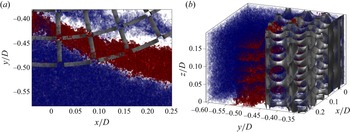
The streamwise velocity fluctuations per mode, $u'(x,y,z,t)|_n$, were run through a fast Fourier transform to generate the power spectral density for mode $n$, $\phi _{u'u'}|_{n}$. Values within 25 % of the maximum value of $\phi _{u'u'}|_{n}$ were calculated and are referred to as $(\phi _{u'u'}|_{n})_{max}$ for convenience. The locations of $(\phi _{u'u'}|_{n})_{max}$ were recorded per mode and are presented in figure 21, where $n = 2$ is presented separately (in red) and other modes $n = 3$ to 10 are presented together (in blue). Modes $n\geq 3$ are presented together to help distinguish mode $n=2$ from other higher-order modes. Layered iso-surfaces of $\phi _{u'u'}|_{n=2}$ are seen to extend through the porous layer into the near-wall region and outer diameter of the SPCC as presented in figure 21(a). The isometric view shown in figure 21(b) reveals clearly visible slices of this spectral content that correspond to the open-pore slices of the SPCC. The region of $n=2$ and propagation trajectory through the porous layer resembles clearly the shear layer trajectory shown in figure 18(a), thereby leading to the conclusion that a boundary layer indeed exists within the porous layer, it separates into a shear layer within the porous layer and contains velocity fluctuations that are linked to vortex shedding from the inner diameter.

Figure 21.

Locations of $(\phi _{u'u'}|_{n})_{max}$ where POD mode $n = 2$ is shown in red and modes $n = 3$–$10$ are shown in blue: (a) $xy$-plane view and (b) arbitrary 3-D view. Flow is in the positive $x$ direction.

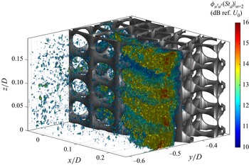
To further understand the development of vortex shedding from the inner diameter, specific values of $\phi _{u'u'}|_{n=2}$ were calculated within the entire FOV 2 domain, being $\phi _{u'u'}(St_{d}=0.19\unicode{x2013}0.22)|_{n=2}$, where the characteristic length used in the Strouhal number calculation is the SPCC inner diameter, $d$. Figure 22 presents these values as iso-surfaces, where the colour scheme represents the $\phi _{u'u'}(St_{d}=0.19\unicode{x2013}0.22)|_{n=2}$ amplitude (dB ref. $U_{0}$). The development of velocity fluctuations related to vortex shedding from the inner diameter is clearly seen to exist within the region identified by the boundary layer thickness and commencement of the separated shear layer. Investigation of higher-order mode spectral content in the vicinity of the SPCC outer diameter, $D$, reveals no clearly observable flow structures related to vortex shedding. Local regions of peak $\phi _{u'u'}(St_{d}=0.19\unicode{x2013}0.22)|_{n=2}$ values coincide with the open-pore areas at the outer diameter, revealing flow instabilities exiting the porous layer into the near-wall flow region (that then propagate beyond the cylinder into the wake). This is identified by the regularly spaced structures that repeat in the $z$ direction (spanwise direction) whose locations match the open-pore regions. The visualisation of this flow phenomenon is only possible by extracting the relevant POD mode ($n=2$) and isolating the spectral content directly related to vortex shedding from the inner diameter. The exit velocity of the $n = 2$ flow field mode is of critical importance, as it is linked to the convective velocity of the disturbances in the shear layer from within the porous layers and originating from the inner diameter.

Figure 22.

Iso-surfaces of the spectral density of streamwise velocity fluctuations of POD mode $n = 2$ in FOV 2 evaluated at $St_{d} = 0.19$ to 0.22, $\phi _{u'u'}(St_{d})|_{n=2}$. Flow is in the positive $x$ direction.

6. Internal vortex shedding development and Strouhal number shift

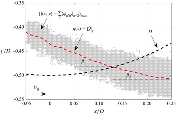
The positions of $(\phi _{u'u'}|_{n})_{max}$ are projected onto a single $xy$ plane to quantify the trajectory of the shear layer through the porous layers and into the near-wall region. This projection, depicted in figure 23, is defined as

(6.1)\begin{equation} Q(x,y) = \sum_{z}(\phi_{u'u'}|_{n=2})_{max}.\end{equation}

Figure 23.

Map of $Q(x,y)$, the mean shear layer trajectory, $q(x) = Q|_{y}$, and angles $\beta _{1}$ and $\beta _{2}$.

Non-zero values of $Q(x,y)$ are averaged along the $y$ axis to obtain a mean shear layer trajectory $q(x)$ (i.e. $q(x) = Q|_{y}$) that propagates (relative to the $x$ axis) with angles $\beta _{1}$ within the porous layer and $\beta _{2}$ immediately outside the porous layer. These angles are calculated via $\beta _{1,2} = \tan ^{-1}(\mathrm {d}q(x)/\mathrm{d}\kern0.06em x)$ using $q(x)$ within and outside the porous layer, respectively, to yield $\beta _{1} = 22^{\circ }$ and $\beta _{2} = 12^{\circ }$. The difference in propagation angles reveals that the porous layers provide a significant impedance that influences the convective disturbance velocity (relative to a bare cylinder) thereby altering the vortex shedding frequency.

The following is proposed: assume that the vortex shedding frequency of the SPCC, $f_{\varPhi }$, is related to the Strouhal number of the inner diameter using the shear layer velocity (carrying the convective disturbances into the wake) instead of the free-stream velocity. The shear layer velocity outside the porous layers is defined as $\alpha _{\varPhi } U_{0}$, where $\alpha _{\varPhi }$ is a constant for a given PCC/SPCC. This assumption (herein referred to as the $\alpha _{\varPhi }$–$U_{0}$ assumption) is based on the different convective disturbance velocities of the SPCC and bare cylinder due to the impedance of the porous layer that carry the convective disturbances into the wake (see figure 22). Replacing $U_{0}$ with $\alpha _{\varPhi } U_{0}$ in the Strouhal number relationship yields

(6.2)\begin{equation} St = \frac{f_{\varPhi}d}{\alpha_{\varPhi}U_{0}}.\end{equation}

Now the Strouhal number of a bare cylinder with diameter $d$ can be substituted into the left-hand side of (6.2) to arrive at

(6.3)\begin{equation} \frac{f_{\varPhi}} {f_{d}} = \frac{\alpha_{\varPhi}}{\alpha_{d}},\end{equation}

where the velocity of the shear layer of a bare cylinder is defined as $\alpha _{d}U_{0}$. Note that (6.2) and (6.3) are independent of $D$ and therefore $\alpha _{\varPhi }$ is specific for each PCC with unique $t/d$ and porous properties. A bare cylinder in the studied Reynolds number range has $\alpha _{d} = 1.15$ (Naito & Fukagata Reference Naito and Fukagata2012; Li et al. Reference Li, Tang, Liu, Arcondoulis and Yang2020b), and for the SPCC investigated here, $\alpha _{\varPhi } = 0.85$. Therefore the ratio of the shear layer velocities is $\alpha _{\varPhi }/\alpha _{d} = 0.7$.

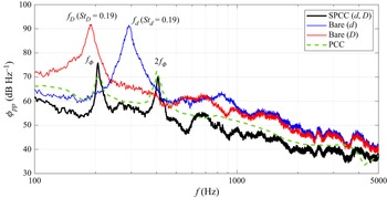
To support the $\alpha _{\varPhi }$–$U_{0}$ assumption, figure 24 presents published bare cylinder (diameters $d$ and $D$), SPCC (Arcondoulis et al. Reference Arcondoulis, Geyer and Liu2021a) and PCC (Zamponi et al. Reference Zamponi, Avallone, Ragni and van der Zwaag2022) far-field acoustic spectra (inner diameter $d$ and outer diameter $D$), where $D = 48$ mm, $d = 32$ mm. For comparison with the SPCC, the data of Zamponi et al. (Reference Zamponi, Avallone, Ragni and van der Zwaag2022) are scaled in the frequency axis to match the Strouhal number shift of their bare $d$ cylinder shedding frequency and scaled in magnitude via a correction of $10\log _{10}(U_{0}^{6})$. By inspection of figure 24 the recorded SPCC far-field spectrum is in excellent agreement with the $\alpha _{\varPhi }$–$U_{0}$ assumption, where $f_{\varPhi }/f_{d} \approx 0.7$. Published numerical data of Li et al. (Reference Li, Tang, Liu, Arcondoulis and Yang2020b) that modelled PCCs with $t/d = 0.25$ and varying PPI from 5 to 80 also agree with the $\alpha _{\varPhi }$–$U_{0}$ assumption. By inspection of their data, a PCC with ${\rm PPI} = 5$ yields $\alpha _{\varPhi }/\alpha _{d} \approx 0.73$ and $f_{\varPhi }/f_{d} \approx 0.73$ (similar PPI and porosity to those of this study), and a PCC with ${\rm PPI} = 10$ yields $\alpha _{\varPhi }/\alpha _{d} \approx 0.55$ and $f_{\varPhi }/f_{d} \approx 0.55$.

Figure 24.

Published far-field acoustic spectra, $\phi _{pp}$ (dB Hz$^{-1}$), of bare cylinders with $d = 32$ mm, $D = 48$ mm, SPCC with $d = 32$ mm, $D = 48$ mm ($t/d = 0.25$) (data obtained from Arcondoulis et al. (Reference Arcondoulis, Geyer and Liu2021a)) and 30 PPI PCC with $d = 20$ mm, $D = 30$ mm ($t/d = 0.25$) (data obtained from Zamponi et al. (Reference Zamponi, Avallone, Ragni and van der Zwaag2022)).

Geyer (Reference Geyer2020) showed that PCCs with much lower porosities and higher airflow resistivity show good agreement with $St_{D}$. This can be explained by a separate flow regime, where the free-stream flow would penetrate the porous layer, but the impedance of the porous layer on the internal flow field would significantly hinder the development of a shear layer within the porous layer (Li et al. Reference Li, Tang, Liu, Arcondoulis and Yang2020b). Any boundary layer within the porous layer would dissipate energy rapidly as turbulent fluctuations in the flow field would disperse within the porous layer. This was observed for PCCs with ${\rm PPI} > 15$ in Li et al. (Reference Li, Tang, Liu, Arcondoulis and Yang2020b). The impedance difference between the internal and external flow regions is too great to allow refraction across the interface, thereby the porous layers trap the fluid (Naito & Fukagata Reference Naito and Fukagata2012) and the external flow passes around a cylinder that can be accurately modelled via $St_{D}$. Understanding and quantifying the critical porous properties, at which these flow regimes change from inner-diameter to outer-diameter shedding, are for future work.

Both the PCC and SPCC exhibit two tones in figure 24, the first referred to as the $f_{\varPhi }$ tone and the second tone being twice the $f_{\varPhi }$-tone frequency (Arcondoulis et al. Reference Arcondoulis, Geyer and Liu2021a,Reference Arcondoulis, Geyer and Liub), i.e. $2f_{\varPhi }$. This two-tone shedding phenomenon has been consistently observed for PCCs with various porous properties (Geyer & Sarradj Reference Geyer and Sarradj2016; Arcondoulis et al. Reference Arcondoulis, Liu, Li, Yang and Wang2019; Zamponi et al. Reference Zamponi, Avallone, Ragni and van der Zwaag2022) of PPI 5 to 30, $\varPhi \gtrapprox 85$% at $Re_{D} \approx 10^{5}$. It is possible that the presence of these strong tones in the PCC/SPCC spectra may be caused by a dual PCC/SPCC vortex shedding process from the inner diameter $d$ and outer diameter $D$. In this study, there is no evidence to suggest that vortex shedding initiates from the SPCC outer diameter. Nonetheless, the relationship between shedding frequencies is briefly discussed here to refute any suggestion of dual shedding mechanisms. Let us assume that both tones are generated using the same characteristic velocity; this is reasonable considering the relatively small difference in peak velocity recorded at the outer diameter in FOV 2 and $\alpha _{\varPhi }U_{0}$. Then the relationship of the shedding frequencies (2.1) is used to arrive at

(6.4)\begin{equation} f_{d} = f_{D}\left(1+2\left(\frac{t}{d}\right)\right),\end{equation}

where it is also assumed that $St_{D} = St_{d}$ which is a sound assumption based on the small variation in Strouhal number in this Reynolds number range (Norberg Reference Norberg2003). For both the PCC and SPCC, $t/d = 0.25$ and substitution into (6.4) yields $f_{d} = (3/2)f_{D}$, meaning that the ratio of the two tone frequencies should be 3/2. This obviously contradicts the frequency relationship of the tones observed in figure 24 and eliminates any feasible flow mechanisms that involve simultaneous vortex shedding from the inner and outer diameters. This conclusion is also reached by Geyer (Reference Geyer2020).

7. Summary and conclusions

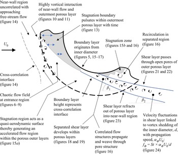
An investigation of the internal and near-wall flow fields of an SPCC was conducted. An SPCC was tested in a water tunnel using flow visualisation and a water flume for TPIV. Flow visualisation was used to qualitatively understand basic internal flow behaviour and four-camera TPIV was used to focus on two fields of view: at the windward and mid-circumference regions. Previously unseen internal flow fields of an SPCC were quantified that are conjectured to be similar to those of typical PCCs that possess similar porosity and airflow resistivity. Vortex shedding originating from the inner diameter is proposed. Strong evidence of velocity fluctuations at the vortex shedding frequency that originate from the inner diameter and exit through individual pores at the outer diameter within the shear layer is observed. A detailed summary of the findings in this study follows the schematic diagram presented in figure 25.

Figure 25.

Schematic diagram identifying key flow features of the SPCC identified from flow visualisation and TPIV.

On the windward side, the primary role of the porous media is to allow the flow to enter the porous layers and to then stagnate in a region significantly larger than that of a bare cylinder. This filling of the porous layer and initiation of stagnation is a short-term transient behaviour that would reach a steady state rapidly, and is not further investigated here. The free-stream flow is then forced around this stagnated flow region, forming an approximate elliptical-shaped geometry. The flow, once passed around the stagnated region, remains attached to the inner diameter and then develops a boundary layer. As the boundary layer grows with respect to circumferential angle, a bare cylinder would normally separate the boundary layer into a separated shear layer at a shallower angle than the SPCC; however, the porous layer now has a secondary role, of keeping the boundary layer attached and providing a flow impedance, such that the boundary layer separates at angle $\beta _{1}$ within the porous layer. The interface between the porous medium and the free-stream medium allows a refraction-like process, in which the wake significantly widens as the shear layer is ejected from the outer porous layer at $\beta _{2}$ and $\alpha _{\varPhi } U_{0}$, as compared with a bare cylinder that would shed a shear layer at a shallower angle and $\alpha _{d} U_{0}$. The SPCC vortex shedding tone frequency can be accurately predicted by assuming that the Strouhal number can be estimated using $\alpha _{\varPhi } U_{0}$ instead of $U_{0}$ (the $\alpha _{\varPhi }$–$U_{0}$ assumption). This assumption leads to the relationship $f_{\varPhi }/f_{d} = \alpha _{\varPhi }/\alpha _{d}$ (equation  (6.3)), where $\alpha _{d}$ can be obtained from abundant published bare cylinder data and then $f_{d}$ can be calculated using the Strouhal number relationship with SPCC inner diameter, $d$. Both the SPCC and published numerical PCC data show excellent agreement with this relationship, giving rise to a promising explanation for the internal vortex shedding mechanism of PCCs.

Understanding the internal flow field of the SPCC opens up several avenues of future work. An upcoming experimental campaign involves testing a series of PCCs and SPCCs with various airflow resistivities and $t/d$ ratios using planar PIV, $f_{\varPhi }$ and $\alpha _{\varPhi }$ values, and further testing the $\alpha _{\varPhi }$–$U_{0}$ assumption. Another ongoing study involves modifying the internal structure of the SPCC at the windward side by replacing the region in which flow stagnation was observed with solid material. This would determine the influence of the flow stagnation on the internal boundary layer (and thus shear layer). From this, the SPCC vortex shedding suppression can be improved via manipulation of the boundary layer and shear layer within the SPCC porous media. Direct numerical simulation of the flow field within the porous media, while presenting a significant computational challenge, would provide the wall pressures on the porous structure and invaluable deeper insight into the internal forces acting on the porous media. Such a detailed analysis could be used to optimise future SPCC designs for passive flow and noise control.