2. THE SETUP

Consider the nonparametric regression

.

Assumption 2.1. The following assumptions are maintained.

(i) The data

are independent and identically distributed (i.i.d.) random variables in

.

(ii) The functional form of

is unknown, but we do know r.

(iii) The conditional pdf of

is twice continuously differentiable at

.

(iv)

, the pdf of

, is twice continuously differentiable at

and

.

(v) For some γ > 0, the map

is bounded and continuous at

.

The restrictions on

, namely, that

is compact and that the last coordinate of

is positive and bounded away from zero, ensure that the conditional expectations in Lemmas 3.1 and 3.2 in Section 3 exist for all

. This allows us to handle any degree of homogeneity. The assumption that we know r is quite weak as economic theory frequently predicts the degree of homogeneity.

is compact, (ii) implies that f is also an element of

. (iii) implies that

are twice continuously differentiable at

. This is used in the proof of Lemma B.1 in Appendix B. We use (iv) to ensure that the remainder terms in the Taylor expansions employed in Appendix A are well behaved. (iv) can be made more palatable if we interpret it to mean that we should carry out estimation and inference in regions where the density is bounded away from zero.

3. ESTIMATION HEURISTICS

Because f is homogeneous of degree r, we can write

The problem we investigate in this paper can be stated quite simply: should we estimate

using the first representation or the second? We refer to the estimator of

based on the first representation as a “projection based” estimator, whereas the estimator based on the second formulation is called a “direct” estimator. It may not be very obvious at this point how we can estimate

using the first representation, but as we shall soon show, it is quite easy to do so. Although algebraically equivalent, the two formulations will in general lead to estimators with different statistical properties because division by x_s^r alters the stochastic properties of the error term ε. In fact, and this should not surprise the reader, the statistical performance of the estimators depends upon the conditional variance

. In particular, we show that if

is homogeneous of degree zero (which includes homoskedasticity as a special case) then the projection based estimator is asymptotically better than the direct estimator, whereas if

is homogeneous of degree 2r ≠ 0 then the latter dominates the former.

Notice that if r = 0, that is, if we are estimating a homogeneous function of degree zero (e.g., a demand function), the two approaches will yield identical results. Furthermore, if s = 1 the problem is uninteresting because homogeneous functions are known up to scale in the one-dimensional case (because when s = 1, homogeneity of f implies that f (x) = x^rf (1)). To avoid these trivial cases, from now on we assume that r ≠ 0 and s > 1.

Our estimation strategy is to approximate sample analogs of optimization problems that identify

using the two representations in (1). At the population level we can use the first representation to write

, where β_p is identified as

Because

is a homogeneous function of degree r for all

, we can characterize

as the orthogonal projection of y onto

using the usual L² inner product

. In particular, we can use Lemma B.2 in Tripathi (2000) to show that this projection can be explicitly calculated as

. This explains the term projection based in describing an estimate obtained by using the first representation in (1). Similarly, a population level specification of

using the second representation can be written as

, where we identify β_d as

Observe that we can also characterize

as the orthogonal projection of y onto

using the “weighted” inner product

. But because this projection is not orthogonal with respect to the usual L² inner product, we prefer to describe

as the “direct” population level specification of

.

The preceding discussion shows that to estimate f, it suffices to estimate β_p and β_d. Because a finite amount of data can at best allow us to estimate the value taken by a function at a certain point, we consider estimating the value of f at

. In particular, let us now see how we can estimate

.

So let β be a function in

that is sufficiently smooth. Think of β as being a generic symbol for β_p or β_d. Taylor expanding

around

and neglecting all higher order remainder terms, we can write

The unknown coefficients

can be estimated by doing least squares on sample analogs of (2) and (3) provided we can maintain the quality of the linear approximation in (4). This can be achieved by employing the usual device of local weighting to ensure that when estimating

, the

closer to

are given more weight than those observations that are farther away from

. Following this approach,

and

can be estimated as

where

.

Here

is the projection based (resp. direct) local linear estimator of

. Similarly,

is the projection based (resp. direct) local linear estimator of its gradient

. The kernel

(defined on

and the bandwidth a_n used previously satisfy the following conditions.

Assumption 3.1.

is a continuous density with support [−1,1] and is symmetric around zero. We also define

.

Assumption 3.2. The bandwidth a_n is a sequence of positive numbers such that a_n → 0, na_n^s−1 → ∞, and na_n^s+3 → λ ∈ [0,∞).

The asymptotic behavior of

is given by the following results.

LEMMA 3.1. Let Assumptions 2.1, 3.1, and 3.2 hold. Then³

Here

denotes a s × 1 vector of zeros.

LEMMA 3.2. Let Assumptions 2.1, 3.1, and 3.2 hold. Then

where bias₁ and bias₂ are defined in Lemma 3.1, and

We use

to denote the projection based and direct local linear estimates of

. Notice that

are homogeneous of degree r by construction; that is, we have obtained homogeneity constrained nonparametric estimators of f. Another nice feature of using the local linear approach is that both

and its partial derivatives can be obtained simultaneously. This comes in handy when one wants to calculate marginal effects or elasticities. Furthermore, solving these optimization problems is straightforward because they can be expressed in a weighted least squares framework. See the proof of Lemma 3.1 in Appendix A for details.

Local linear estimators of conditional mean functions, without any homogeneity restrictions, have been extensively studied. See, for instance, Fan (1992), Ruppert and Wand (1994), Gozalo and Linton (2000), and the references therein. If instead of a first-order approximation in (4) we had taken an mth-order Taylor expansion of

around

, where m > 1, we would have obtained mth-order local polynomial estimators of β_p and β_d. In our case such higher order approximations are unnecessary because a linear approximation suffices to compare the asymptotic mse of

. Of course, we could also have obtained locally constant (better known as Nadaraya–Watson) estimators of

by considering the “zeroth”-order approximation

in (4). In fact, it is easy to show that the projection based and direct Nadaraya–Watson estimators of

are given by

The reason we prefer working with local linear estimators, rather than the locally constant estimators, is that the asymptotic bias terms for the former are simpler (and thus much easier) to handle analytically. In particular, as shown in Lemmas 3.1 and 3.2, they do not have any terms involving the first derivatives of

:

Hence when local linear estimators are used, comparing the asymptotic mse of

reduces to comparing their asymptotic variances. In contrast, in Appendix B it is shown that for the Nadaraya–Watson estimators of

,

Although in Appendix B we also show that

and

, the squared bias of

cannot be ranked. Therefore, if we use Nadaraya–Watson estimators we cannot analytically compare the projection based estimator with the direct estimator in terms of asymptotic mse.

Finally, let

denote the usual unrestricted local linear estimator of

in the regression model

, that is,

where

is an appropriate kernel on

and the bandwidth b_n is a sequence of positive numbers such that b_n → 0 and nb_n^s → ∞. Note that when f is homogeneous of degree r,

will converge at a slower rate to f than

. Imposing homogeneity on estimators of f reduces the dimension of the regressor space by one and leads to estimators with improved rates of convergence. In the simulations we will compare the finite sample behavior of

with

.

4. COMPARING

Following Lemmas 3.1 and 3.2, it is easy to see that the asymptotic variances of

are

To simplify the form of these variances, observe that the transformation

is one to one and apply iterated expectations. This yields

where

is the conditional variance function. It does not seem possible (at least to us) to compare the two variances if

is completely unknown. However, we can obtain some useful insights about the asymptotic variance of

satisfies the following assumption.

Assumption 4.1. Assume that either

(i)

for some unknown ψ; that is, the error terms are conditionally heteroskedastic such that

is homogeneous of degree zero in the covariates, or

(ii)

for some unknown ψ; that is, the error terms are conditionally heteroskedastic such that

is homogeneous of degree r ≠ 0 in the covariates.

Notice that Assumption 4.1(i) is automatically satisfied if the error term is homoskedastic. As an example of a model where homoskedasticity of ε is compatible with linear homogeneity of f, consider the following simple setup.

Example 4.1.

Let y be the observed profit, f the unobserved profit function of a competitive firm, and

the vector of observed output and factor prices. Assuming that the prices are measured without error but there is measurement error in the observed profit, we can write

. Because f is a profit function it is homogeneous of degree one, and as ε is treated as pure measurement error we can assume that it is homoskedastic.

Although homoskedasticity of additive errors is often a convenient statistical assumption, it is sometimes hard to justify from a structural point of view. In many cases, Assumption 4.1(ii) may be more plausible. As an example of a situation where both

are homogeneous of degree one, consider the following model, which is motivated by the discussion in McFadden (1984, p. 1406).

Example 4.2.

Let

be the vector of observed output and factor prices and

the unobserved profit function of a competitive firm. The term u denotes a firm specific random parameter that is distributed independently of

. It is unobserved by the researcher but is known to the firm itself. For instance, u could represent variables that are unobserved by the economist but are used by the firm when making production decisions. Because f* is a profit function, we assume that for each u ∈ U the map

is linearly homogeneous, monotone, and convex in the prices. Let

denote the maximum observable profit. Then using the fact that u is independent of

, we can write

where

and

Note that

has all the properties of a profit function. In particular, it is homogeneous of degree one. Moreover, we can also verify that

and that

is homogeneous of degree one.

Now it is easy to see that

Hence the expressions for the asymptotic variances simplify to

Because by the Cauchy–Schwarz inequality

we get that

under Assumption 4.1(i), and

under Assumption 4.1(ii). As the asymptotic bias for the two estimators is identical, we have

under Assumption 4.1(i) and

under Assumption 4.1(ii). Therefore, as expected there is no general ranking for the estimators in terms of asymptotic mse. Hence the choice of which estimator to use is not obvious but depends upon the nature of the heteroskedasticity of the error term.

5. SIMULATION

A small simulation experiment was performed to study the finite sample properties of the proposed estimators. Code was written in GAUSS, and we restricted our attention to the case s = 2. A number n of observations on y were generated from y = f (x₁,x₂) + σ(x₁,x₂)ε, where

and ε was chosen independently of (x₁,x₂). A Gaussian kernel was used to obtain

. For the first two estimators the bandwidth used was cn^−1/5, whereas for

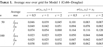
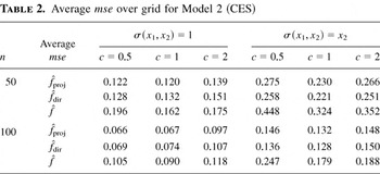
the bandwidth used was cn^−1/6. Three different choices of c were considered: c ∈ {0.5,1,2}. As seen in Tables 1 and 2, the results do not seem to be very sensitive to the choice of bandwidth. Two particular specifications for f and ε were selected:

The terms f₁ and f₂ represent a Cobb–Douglas and constant elasticity of substitution (CES) specification, respectively. Note that both f₁ and f₂ are homogeneous of degree one. The model parameters were chosen so that var{f (x₁,x₂)}/var{y}, which can be thought of as a measure of the S/(S + N) ratio, for each model is around 0.8. Two simple forms for σ(x₁,x₂) were chosen to satisfy Assumption 4.1: σ(x₁,x₂) = 1, which satisfies 4.1(i), and σ(x₁,x₂) = x₂, which satisfies 4.1(ii). Each function was estimated at a 10 × 10 uniform grid in [1,2] × [1,2] and the mse calculated at each grid point in 1,000 replications.

Average mse over grid for Model 1 (Cobb–Douglas)

Average mse over grid for Model 2 (CES)

Recall that our asymptotic results are about the pointwise behavior of the mse. But because the reader may find point by point comparison of mse on the 10 × 10 grid a tedious task, we present the average (over 100 grid points) mse in Tables 1 and 2.

As seen in the tables, the average mse is ranked according to our asymptotic results. Moreover, except in one case

For Model 2 when n = 100 and c = 2. However, a decomposition of the average mse for this case revealed that although the average variance for

was smaller than the average variance of

, the average squared bias for the former was bigger than the average squared bias for the latter. Therefore, although the ranking with respect to the variances is preserved according to our theory, the average bias differs for the two models. Hence, in this case the higher average bias of

caused the ranking to change.

dominates, although there does not seem to be a dramatic difference between

in terms of average mse. When the conditional variance of ε is homogeneous of degree one,

has the smallest average mse although once again the difference between

is not very substantial. However, in each case the homogeneity constrained estimators clearly outperform

, the unrestricted local linear estimator of f. Therefore, when f is indeed homogeneous, using a homogeneity constrained estimator seems sensible. Of course, the reader must keep in mind the usual caveat about any simulation results, namely, that they are limited in nature and may vary if the underlying model parameters are changed.