Implications
A generic model for beef cattle, named LiGAPS-Beef (Livestock simulator for Generic analysis of Animal Production Systems – Beef cattle), has been described and illustrated in a companion paper (Van der Linden et al., Reference Van der Linden, Van de Ven, Oosting, Van Ittersum and De Boer2018a). This mechanistic model aims to assess the potential (i.e. theoretical maximum) and feed-limited growth and production of cattle in different beef production systems across the world. In this paper, we conducted sensitivity analyses and evaluated parts of LiGAPS-Beef with independent experimental data. Our results contribute to the evidence that LiGAPS-Beef can be used to simulate beef production in a broad range of systems with different climates and feeding strategies.
Introduction
The increasing demand for animal-source food calls for insight to what extent livestock production can be increased in different parts of the world. The biophysical scope to increase livestock production is the difference between the potential (i.e. maximum theoretical) production or feed-limited production and the actual production realized in practice, which is also referred to as the yield gap (Van de Ven et al., Reference Van de Ven, de Ridder, van Keulen and van Ittersum2003; Van der Linden et al., Reference Van der Linden, Oosting, Van de Ven, De Boer and Van Ittersum2015). Identifying geographical regions with large yield gaps contributes to insight where food production can be increased per unit of land, which is generally regarded as a better strategy than expanding agricultural land at the expense of nature (Lobell et al., Reference Lobell, Cassman and Field2009; Van Ittersum et al., Reference Van Ittersum, Cassman, Grassini, Wolf, Tittonell and Hochman2013).
Yield gaps of arable crops are widely assessed with mechanistic crop growth models, which simulate potential and water-limited production in different farming systems and in different regions of the world (Jones et al., Reference Jones, Hoogenboom, Porter, Boote, Batchelor, Hunt, Wilkens, Singh, Gijsman and Ritchie2003; Keating et al., Reference Keating, Carberry, Hammer, Probert, Robertson, Holzworth, Huth, Hargreaves, Meinke, Hochman, McLean, Verburg, Snow, Dimes, Silburn, Wang, Brown, Bristow, Asseng, Chapman, McCown, Freebairn and Smith2003). Yield gaps of livestock have not been assessed with mechanistic models yet, since models simulating potential and feed-limited livestock production were hardly available at the start of this research. A generic, mechanistic model was developed, therefore, to assess potential and feed-limited beef production in different beef production systems and in different regions of the world (Van der Linden et al., Reference Van der Linden, Van de Ven, Oosting, Van Ittersum and De Boer2018a). This model is named LiGAPS-Beef, and its results may eventually contribute to the identification of regions with a large biophysical scope to increase beef production.
Mechanistic models include the most important processes and mechanisms in systems, but still consist of multiple empirical elements and parameters that can considerably affect model output, and subsequently the conclusions based on the models’ output (Thornley and France, Reference Thornley and France2007). Sensitivity analysis provides insight in how model output is affected by changes in model input. This method ranks input parameters based on their effect on model output (Pianosi et al., Reference Pianosi, Beven, Freer, Hall, Rougier, Stephenson and Wagener2016). Ranking parameters can be used to prioritise which parameters need to be estimated more precisely (Zuidema et al., Reference Zuidema, Leffelaar, Gerritsma, Mommer and Anten2005). Sensitivity analysis is of particular importance if models are applied outside conditions they were calibrated for (Prisley and Mortimer, Reference Prisley and Mortimer2004). Since LiGAPS-Beef is designed to be applicable to a broad range of beef production systems, conducting sensitivity analysis is essential.
Furthermore, key processes in the model must be simulated in sufficient detail to ensure applicability of the model under a wide range of agro-ecological conditions and beef production systems. If key processes are simulated in sufficient detail, model output must resemble experimental data. Hence, model evaluation with experimental data is an essential and necessary step after model development to investigate whether model output is accurate. Model evaluation is conducted with experimental data not used for model calibration, so experimental data for model calibration and evaluation are independent (Bellocchi et al., Reference Bellocchi, Rivington, Donatelli and Matthews2010). Model evaluation with independent experimental data is also referred to as model validation or testing, but we will use the term model evaluation consistently throughout this paper. Given the relevance of sensitivity analysis and model evaluation, the first aim of this paper is to assess which model parameters affect model output most. The second aim is to evaluate the performance of LiGAPS’ sub-models on thermoregulation and feed intake and digestion with independent experimental data. The performance of the complete model LiGAPS-Beef in different beef production systems is evaluated in a companion paper (Van der Linden et al., Reference Van der Linden, Van de Ven, Oosting, Van Ittersum and De Boer2018b).
Material and methods
Structure of LiGAPS-Beef
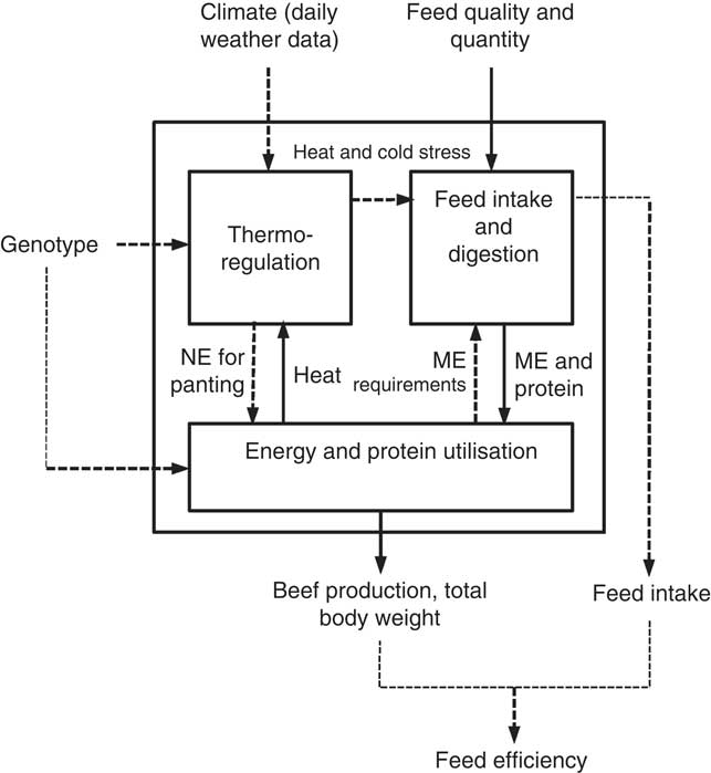
LiGAPS-Beef consists of a thermoregulation sub-model, a feed intake and digestion sub-model, and an energy and protein utilisation sub-model (Van der Linden et al., Reference Van der Linden, Van de Ven, Oosting, Van Ittersum and De Boer2018a) (Figure 1). The thermoregulation sub-model simulates heat release, based on existing thermoregulation models (McGovern and Bruce, Reference McGovern and Bruce2000; Turnpenny et al., Reference Turnpenny, McArthur, Clark and Wathes2000a). This sub-model requires daily weather data if cattle are kept outdoors and climate conditions in stables if cattle are housed (Figure 1). Genetic parameters and heat production from metabolic processes are inputs too. Minimum and maximum heat release are outputs of this sub-model. Cold conditions can increase feed intake, whereas hot conditions can decrease feed intake. The thermoregulation sub-model increases energy requirements under hot conditions, because energy is spent on panting (Figure 1). Inputs for the feed intake and digestion sub-model are the energy requirements of cattle and the quality and quantity of the available feeds (Figure 1). Feed intake is an output of this sub-model. Feed digestion is simulated based on a rumen model of Chilibroste et al. (Reference Chilibroste, Aguilar and Garcia1997), and yields metabolisable energy (ME) and digested protein as major outputs, which are used as input for the energy and protein utilisation sub-model. Energy and protein are distributed over the metabolic processes maintenance, physical activity, growth, gestation, and lactation (Van der Linden et al., Reference Van der Linden, Van de Ven, Oosting, Van Ittersum and De Boer2018a). Energy and protein for growth are allocated to different tissues (non-carcass tissue, and bone, muscle and fat tissue in the carcass). Beef is defined as deboned carcass. Feed efficiency of individual animals (FE, g beef/kg DM feed) is calculated from their beef production and feed intake (Figure 1). Results for individual animals can be scaled up to the herd level.
Representation of LiGAPS-Beef (Livestock simulator for Generic analysis of Animal Production Systems – Beef cattle) and the connections among the three sub-models. Solid arrows indicate flows of material or energy in beef cattle, dashed arrows indicate a flow of information. ME=metabolisable energy; NE=net energy. Source: van der Linden et al. (Reference Van der Linden, Van de Ven, Oosting, Van Ittersum and De Boer2018a).

Sensitivity analysis
Thermoregulation sub-model
Sensitivity analysis was used to assess the effect of changing parameters and weather data on the lower critical temperature (LCT) and upper critical temperature (UCT) simulated by the thermoregulation sub-model. In total, 31 parameters were investigated (23 cattle-specific; 8 breed-specific). These parameters were decreased and increased by 10%, while all other parameters were kept at their original values, according to the one-at-a-time approach (Pianosi et al., Reference Pianosi, Beven, Freer, Hall, Rougier, Stephenson and Wagener2016). Two exceptions were the body temperature (which was changed by 1°C, or 2.6%) and the standard temperature used in the formula to calculate the latent heat release from the skin (which was changed by 1%), because changing these two parameters by 10% caused excessive heat stress, which resulted in a reduction of feed intake, and eventually a complete depletion of the body fat reserves. We concluded, therefore, that changes of 10% were beyond the feasible biological range. Chemical and physical parameters were not included in the sensitivity analysis, since they were considered constants. In the baseline scenario for sensitivity analysis, solar radiation was set at 10 MJ/m2 coat per day, relative humidity at 50%, wind speed at 4 m/s, precipitation at 0 mm/day and cloud cover at 4okta. The total BW (TBW) was 450 kg in the baseline scenario, and heat production was 1.36 times maintenance heat production for Bos taurus cattle, which corresponds to a situation where approximately half of the ME is allocated to maintenance, and half to growth. In addition, we investigated the LCT and UCT within a range of temperatures (−40°C to 40°C) combined with a range of solar radiation levels (0 to 30 MJ/m2per day), relative humidity levels (10% to 100%), wind speeds (0.1 to 8.0 m/s), precipitation levels (0 to 30 mm/day) and cloud cover levels (0 to 8okta). In addition, the range of temperatures was combined with a range of TBWs (50 to 1300 kg) and heat production levels (1.0 to 2.0×maintenance heat production).
Feed intake and digestion sub-model
Feed intake is dependent on the genotype of the animal, the climate, feed quality and the available feed quantity, and is, therefore, an output of the joint sub-models of LiGAPS-Beef (Figure 1). Feed digestion can be investigated with the feed intake and digestion sub-model only. The output of this sub-model is the ME content (MJ/kg DM) and digestible protein content (g/kg DM) of particular feeds and diets, using feed constituents as model inputs. Feed constituents investigated were soluble, non-structural carbohydrates (SNSC), insoluble, non-structural carbohydrates (INSC), digestible NDF (DNDF), soluble CP (SCP), digestible CP (DCP) and total CP (Chilibroste et al., Reference Chilibroste, Aguilar and Garcia1997). In addition, digestion (3×) and passage rates (2×) were included, as well as the slope and intercept of a Lucas equation (equation (1)) (Lucas et al., Reference Lucas, Smart, Cipolloni and Gross1961; Van Soest, Reference Van Soest1994). Feed constituents of 13 feeds were decreased by 10% to investigate the effect on ME and digestible protein content using the one-at-a-time approach.
 $$\scale 95% { {\rm Digestible}\,{\rm protein}\left( {{\rm g\,/\,kg}\,{\rm DM}} \right)\; {\equals}\; 0.9{\times}{\rm CP}\left( {{\rm g\,/\,kg}\,{\rm DM}} \right)-32$$
LiGAPS-Beef
Sensitivity analysis was conducted to assess the effect of changing parameters on FE at the herd level. Sensitivity analysis (one-at-a-time approach) was conducted for all parameters of LiGAPS-Beef, including the 31 parameters from the thermoregulation sub-model, and the slope and intercept of the Lucas equation (equation (1)). Parameters were decreased and increased by both 5% and 10%. The arbitrary changes of 5% and 10% were chosen because the standard deviations of parameters or their expected range are unknown for most parameters. The disadvantage of this approach is that the decrease or increase of parameters can be outside their biologically feasible range, and consequently no meaningful model output is obtained. Three parameters were changed by less than 5%, since biological limits did not allow a change of 5% and 10%. The standard temperature used in the formula to calculate the latent heat release from the skin and a parameter to calculate body area were changed by 1%, and the body core temperature was changed by 0.1°C. Parameters of the Gompertz curve were changed together because they are interrelated, except for the rate constant. The sensitivity of model output was represented by the sensitivity coefficient, which is the ratio of change in model output to the change in the parameter value (Hamby, Reference Hamby1994).
Sensitivity analysis was conducted at the herd level for ¾ Brahman×¼ Shorthorn (B×S) cattle, adapted to a tropical climate, and for Hereford cattle, adapted to a temperate climate. Four hypothetical baseline scenarios were used for the sensitivity analysis: B×S cattle in Australia under potential production; B×S cattle in Australia under feed quality limited production; Hereford cattle in Uruguay under potential production; and Hereford cattle in Uruguay under feed quality limited production. Under potential production, cattle were permanently housed, and the diet consisted of wheat (65%) and good quality hay (35%). Under feed quality limitation, the ME content of the diet was set at 11.1 to 12.2 MJ/kg DM in Australia, and 10.7 to 11.8 MJ/kg DM in Uruguay. Weather data used were from the year 1992 in Australia and 2002 in Uruguay. Weaning age was set at 210 days in both countries. The culling rate for a cohort of cows after the birth of the first calf was set at 50% per year (Van der Linden et al., Reference Van der Linden, Oosting, Van de Ven, De Boer and Van Ittersum2015 and Reference Van der Linden, Van de Ven, Oosting, Van Ittersum and De Boer2018a). As cows were assumed to conceive up to an age of 10 years, each cow gives, on average, birth to two calves. The female calf is used as a replacement for the reproductive cow and is not part of the herd unit, but gives rise to the next one (Van der Linden et al., Reference Van der Linden, Oosting, Van de Ven, De Boer and Van Ittersum2015 and Reference Van der Linden, Van de Ven, Oosting, Van Ittersum and De Boer2018a). Hence, one herd unit consists of a reproductive cow and one male calf. Slaughter weights of male B×S and Hereford calves were optimised to maximise FE at the herd level (Van der Linden et al., Reference Van der Linden, Van de Ven, Oosting, Van Ittersum and De Boer2018a).
Evaluation of sub-models
The thermoregulation sub-model and the feed intake and digestion sub-model were each evaluated with independent experimental data. The energy and protein utilisation sub-model is the largest and central sub-model, and it requires a significant amount of inputs from the thermoregulation and feed intake and digestion sub-model (Figure 1). For this reason, evaluation of the energy and protein utilisation sub-model was not conducted in this paper. Evaluation of this large sub-model is, however, included indirectly in the evaluation of LiGAPS-Beef as a whole, which is reported in a companion paper (Van der Linden et al., Reference Van der Linden, Van de Ven, Oosting, Van Ittersum and De Boer2018b).
Thermoregulation sub-model
The thermoregulation sub-model was calibrated, since its daily time step was much coarser than the time step used in the thermoregulation models of McGovern and Bruce (Reference McGovern and Bruce2000) and Turnpenny et al. (Reference Turnpenny, McArthur, Clark and Wathes2000a). Model simulations included an animal of 450 kg TBW kept outdoors. Solar radiation levels were set at 15 MJ/m2 per day (horizontal surface), which was assumed to correspond to 7.5 MJ/m2 coat per day. Cloud cover was set at 4 okta, and the level of precipitation at 0 mm/day. Parameters for respiration and latent heat release from the skin were adjusted to fit to temperature–humidity indices (equations (2) and (3)) (Mader et al., Reference Mader, Davis and Brown-Brandl2006).
 $${\rm THI}{\; \equals}\; 0.8{\times}T{\plus}{\rm RH}\,/\,100{\times}\left( {T{\minus}14.4} \right){\plus}46.4$$
 $${\rm THI}_{{{\rm adj}{\rm .}}} {\; \equals\; }{\rm THI}{\plus}4.51{\minus}1.992{\times}{\rm WS}{\plus}0.0068{\times}{\rm SR}$$
Where THI is the temperature–humidity index, T the temperature (°C), RH the relative humidity (%), THIadj. the temperature–humidity index adjusted for wind speed and solar radiation, WS the wind speed (m/s) and SR the level of solar radiation (W/m2). Threshold values for THI and THIadj. were adopted from Mader et al. (Reference Mader, Davis and Brown-Brandl2006). After calibration, simulated heat release was compared with measured heat release from two experiments, which were also used to calibrate the model of Turnpenny et al. (Reference Turnpenny, McArthur, Clark and Wathes2000a). In the first experiment, heat release of Aberdeen Angus×Shorthorn steers (323 to 361 kg TBW) was measured at low temperatures (−1.1°C to 3.1°C), with low (<7 mm) and high coat lengths (>24 mm) (Blaxter and Wainman, Reference Blaxter and Wainman1964). In the second experiment, heat release of Friesian calves (initial TBW 34.6 kg) and Jersey calves (initial TBW 27.8 kg) was measured for a range of temperatures (3°C to 20°C) and two wind speeds (0.22 and 1.56 m/s) (Holmes and McLean, Reference Holmes and McLean1975). Coat length was not measured in this experiment, but it was assumed to be 25 mm. In both experiments, animals were expected to be below their LCT in most of the experimental treatments, and hence their measured heat release should correspond to the minimum heat release simulated with the thermoregulation sub-model.
Feed intake and digestion sub-model
We used the seven feed constituents and their digestion and passage rates specified by Chilibroste et al. (Reference Chilibroste, Aguilar and Garcia1997) as input to simulate the ME content of 13 feed types (MJ/kg DM). Simulated ME contents were compared with measured ME contents from Ministry of Agriculture, Fisheries & Food (MAFF) (1986) and Kolver (Reference Kolver2000). The mean absolute error (MAE) (equation (4)), mean square error (MSE) and the RMSE (equation (5)) reflect the deviation of simulated ME contents from the measured ME contents. The MSE was decomposed into the bias, slope and random component (Bibby and Toutenburg, Reference Bibby and Toutenburg1977). The bias component indicates systematic errors in the model, and the slope component indicates the models’ ability to replicate the variability in the measured data. The random component is the remaining variation after accounting for the bias and slope components (Bibby and Toutenburg, Reference Bibby and Toutenburg1977). A perfect fit of the regression line between simulated and measured data means that the bias and slope components explain 0% of the MSE, and the random component 100% (Bellocchi et al., Reference Bellocchi, Rivington, Donatelli and Matthews2010).
 $${\rm MAE}{\; \equals\; }{{\Sigma \left| {O-S} \right|} \over n}$$
 $${\rm RMSE}{\; \equals\; }\sqrt {{{\Sigma \left( {O-S} \right)^{2} } \over n}} $$
Where O is the observed value, S the simulated value and n the number of observations. The measured and simulated digested protein were not compared with each other, because the CP content of feeds given in Chilibroste et al. (Reference Chilibroste, Aguilar and Garcia1997) was often different from the CP content given in MAFF (1986).
Results
Sensitivity analysis
Thermoregulation sub-model
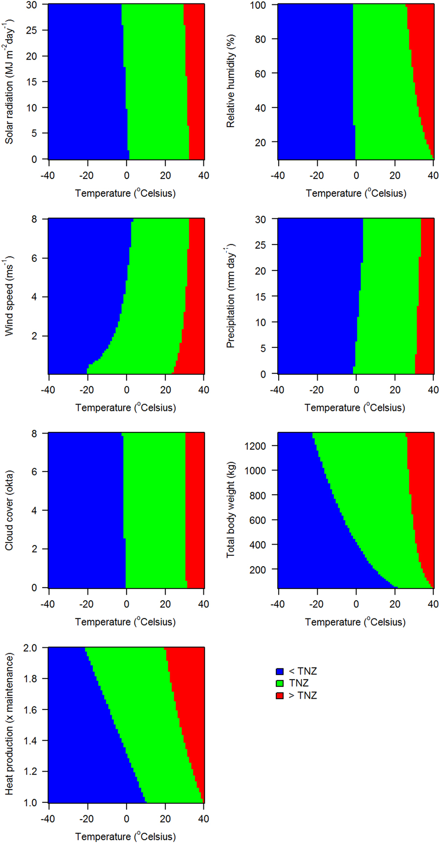
The LCT was affected by more than 1.0°C for parameters used to calculate the body area and the minimum conduction between body core and skin (three parameters) (Table 1). The UCT was affected by more than 1.0°C for parameters used to calculate the body area, body temperature, exhaled air temperature, maximum conduction between body core and skin, and latent heat release from the skin (two parameters) (Table 1). The LCTs and UCTs decreased with increasing solar radiation, relative humidity, TBW and heat production, whereas they increased with increasing wind speed and precipitation (Figure 2). The ranges used for wind speed, TBW and heat production resulted in considerable shifts in the LCTs and UCTs (10°C or more for the LCT). Changes in relative humidity mainly affected the UCT, and hardly the LCT (Figure 2). The shifts in LCT and UCT within the ranges specified were generally larger than the changes in LCT and UCT after changing parameters by 10% (Figure 2, Table 1).
(colour online) Effects of temperature in combination with solar radiation, relative humidity, wind speed, precipitation, cloud cover, total BW and heat production on the simulated thermal neutral zone (TNZ) (in white) of a bovine animal. The lower critical temperature of the cattle is the left edge of the TNZ; the upper critical temperature the right edge.

Changes in lower critical temperature (LCT) and upper critical temperature (UCT) of beef cattle after changing parameters by 10%. The baseline LCT is −1.0°C and the baseline UCT is 30.5°C. Changes (only 1°C or more) are given in degrees Celsius, relative to the baseline

1 Body area (m2)=body area multiplier×body area 1×total BWbody area 2 (McGovern and Bruce, Reference McGovern and Bruce2000).
2 Body temperature has been changed by 1°C.
3 Minimum conduction core-skin (W/m2 per K)=conduction core-skin 1/(conduction core-skin 2×TBWConduction core-skin 3).
4 Maximum latent heat release (W/m2)=minimum heat release+latent heat release 1×e (latent heat release 2×(skin temperature−latent heat release 3))×latent heat of water vapour.
5 This parameter has been changed by 1%.
Feed intake and digestion sub-model
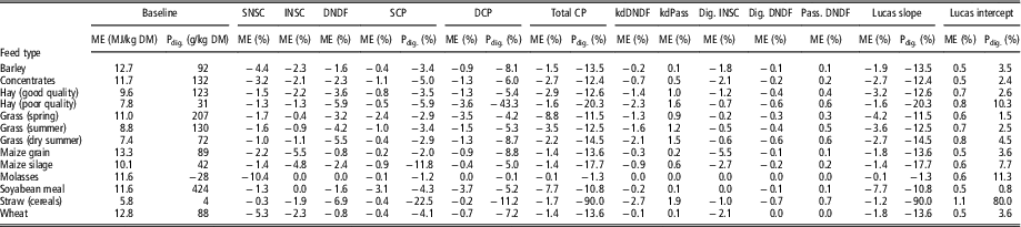
Reducing the content of SNSC, INSC, DNDF, SCP, DCP and total CP by 10% resulted in a lower ME and digestible protein content for all feed types (Table 2). The ME content increased upon a 10% reduction in the passage rate in the rumen, the passage rate for DNDF, and the intercept of the Lucas equation (equation (1)). The SNSC content affected the ME content of molasses (−10.4%), wheat (−5.3%), barley (−4.4%) and concentrates (−3.2%) most (Table 2). The DNDF content affected the ME content of cereal straw (−6.9%), hay (up to −5.9%) and grass (up to −5.5%) most. Decreasing the slope of the Lucas equation had the same effect on the amount of digestible protein as decreasing the total CP content of the feed (Table 2). The digestible protein content of all feeds was negatively affected by a decrease in the slope of the Lucas equation, and positively by a decrease in its intercept. For molasses, the amount of protein digested in the baseline was negative, because the Lucas equation is negative at low levels of CP (4 g/kg DM for molasses). Its intercept and slope affected the digestible protein content of feeds with low CP contents (+80% and −90% for cereal straw) to a larger extent than feeds with high CP contents (+1% and −11% for soyabean meal) (Table 2).
Effect of a 10% decrease in feed components on metabolisable energy (ME) and digested protein (Pdig.) per kg DM feed

SNSC=soluble, non-structural carbohydrates; INSC=insoluble, non-structural carbohydrates; DNDF=digestible NDF; SCP=soluble CP; DCP=digestible CP; kdDNDF=digestion rate digestible NDF; kdPass=passage rate; Dig. INSC=digestion rate of insoluble, non-structural carbohydrates for the whole digestive tract; Dig. DNDF=digestion rate of degradable NDF in the intestines; Pass. DNDF=passage rate of degradable NDF in the intestines; Lucas slope and intercept=slope and intercept of a Lucas equation (equation (1), Lucas et al., Reference Lucas, Smart, Cipolloni and Gross1961; van Soest, Reference Van Soest1994).
Baseline ME and Pdig. indicate the whole-tract digestibility for beef cattle. Other values indicate the relative change in ME and Pdig. compared with the baseline (%).
LiGAPS-Beef
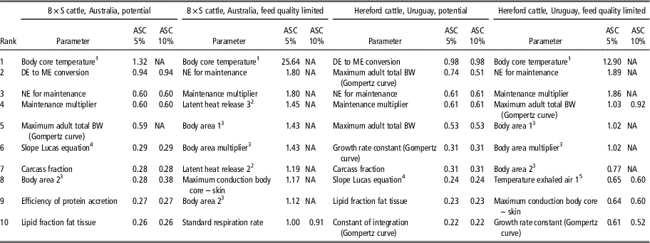
For the baseline scenario, the FE of B×S cattle in Australia was 77.0 g beef/kg DM (65% wheat, 35% good quality hay) under potential production and 40.8 g beef/kg DM (pasture) under feed quality limited production. The FE of Hereford cattle in Uruguay was 71.4 g beef/kg DM under potential production and 37.1 g beef/kg DM under feed quality limited production. Changing parameter values by 5% or 10% hardly affected the FE at the herd level for most of the parameters under potential production. The sensitivity coefficient was only higher than one for the body temperature of B×S cattle in Australia, whereas sensitivity coefficients were below one for Hereford cattle in Uruguay (Table 3). Six parameters in the top-10 parameters affecting model output most were found both in Australia and Uruguay under potential production. The net energy (NE) for maintenance and its multiplier were in the top-10 parameters for each of the four scenarios. Sensitivity coefficients were higher under feed quality limited production than under potential production. Changing parameters in the top 10 by 10% often did not result in meaningful output under feed quality limited production, due to simulated heat stress, the consequent reductions in feed intake, depletion of body fat reserves and eventually mortality (Table 3).
Average sensitivity coefficient (ASC) of the top-10 parameters affecting the feed efficiency of beef cattle at the herd level most. Sensitivity analysis was conducted with LiGAPS-Beef (Livestock simulator for Generic analysis of Animal Production Systems – Beef cattle) by increasing and decreasing parameters values by 5% (ASC 5%) and 10% (ASC 10%)

B×S=Brahman×Shorthorn crossbred cattle; DE=digestible energy; ME=metabolisable energy; NA=no model output; NE=net energy.
1 Body core temperature was decreased and increased by 0.1°C.
2 Maximum latent heat release (W/m2)=minimum heat release+latent heat release 1×e (latent heat release 2×(skin temperature−latent heat release 3))×latent heat of water vapour. Latent heat release 3 was changed by 1%.
3 Body area (m2)=body area multiplier×body area 1×total BWbody area 2 (McGovern and Bruce, Reference McGovern and Bruce2000). Body area 2 was changed by 1%.
4 For the Lucas equation, see equation (1).
5 Temperature exhaled air=temperature exhaled air 1+temperature exhaled air 2×air temperature+e (temperature exhaled air 3×relative humidity+temperature exhaled air 4×air temperature).
Parameters related to heat release were listed more often in the top 10 under feed quality limited production than under potential production. Latent heat release (Australia only), standard respiration rate (Australia only), maximum conduction between body core and skin, and the temperature of exhaled air (Uruguay only) were found in the top 10 under feed quality limited production, but not under potential production (Table 3). Sensitivity coefficients were similar for changes of 5% and 10% in parameters under potential production in Australia, which suggests rather linear relations between parameters values and model output. The same holds for Uruguay, except for the adult weight used in the Gompertz curve, where sensitivity coefficients differ for a 5% change and a 10% change (Table 3).
Evaluation of sub-models
Thermoregulation sub-model
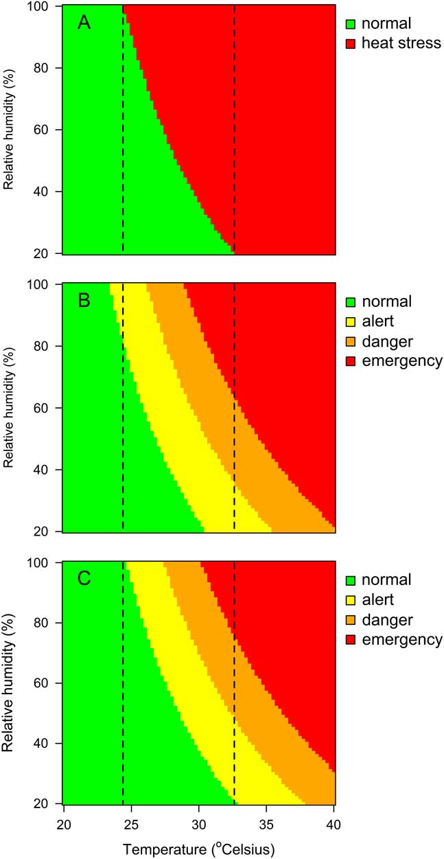
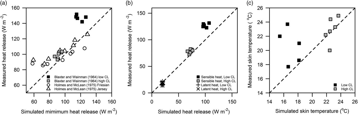
After calibration, the climate conditions resulting in heat stress in the thermoregulation sub-model corresponded to the climate conditions classified as alert, danger and emergency by the temperature–humidity indices (equations (2) and (3)) (Figure 3). Measured heat release and simulated minimum heat release for the experiment of Blaxter and Wainman (Reference Blaxter and Wainman1964) were in agreement for steers with high coat lengths, but simulations underestimated the minimum heat release for steers with low coat lengths (Figure 4a). Measured heat release and simulated minimum heat release of Friesian and Jersey calves for the experiment of Holmes and McLean (Reference Holmes and McLean1975) corresponded to each other at a heat release of ~90 W/m2 and higher (Figure 4a). Treatments at 20°C and at 12°C with a wind speed of 0.22 m/s resulted in a heat release below 90 W/m2. Latent and sensible heat release for the experiment of Blaxter and Wainman (Reference Blaxter and Wainman1964) were simulated well for steers with high coat lengths, whereas sensible heat release was underestimated for steers with low coat lengths (Figure 4b). Simulated and measured skin temperatures for the steers were assessed reasonably well by the thermoregulation sub-model (Figure 4c). Skin temperature was underestimated considerably for one animal having low coat lengths (measured 23.7°C and 22.0°C; simulated 16.5°C and 15.4°C).
(colour online) Combined temperature and relative humidity to compare the occurrence of heat stress in beef cattle simulated by the thermoregulation sub-model of LiGAPS-Beef (Livestock simulator for Generic analysis of Animal Production Systems – Beef cattle) after calibration (a) with the temperature–humidity index of Mader et al. (Reference Mader, Davis and Brown-Brandl2006) (b) and the temperature–humidity index of Mader et al. (Reference Mader, Davis and Brown-Brandl2006) accounting for wind speed and solar radiation (c). Dashed lines indicate the simulated temperature at which heat stress occurs with a relative humidity of 20% and 100%.

Simulated and measured total heat release of beef cattle for experiments of Blaxter and Wainman (Reference Blaxter and Wainman1964) and Holmes and McLean (Reference Holmes and McLean1975) (a), together with sensible and latent heat release (b) and skin temperature (c) for the experiment of Blaxter and Wainman (Reference Blaxter and Wainman1964). Dashed lines indicate y=x. CL=coat length.

Feed intake and digestion sub-model
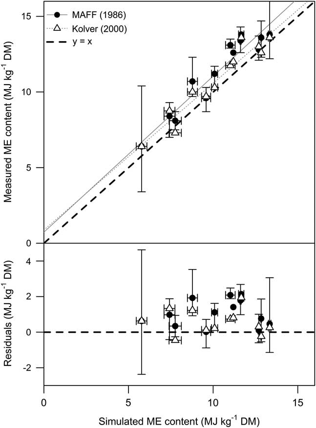
Simulated and measured ME contents of MAFF (1986) generally corresponded to each other (RMSE=1.28 MJ ME/kg DM, MSE=1.64 MJ2 ME/kg2 DM). The MAE was 1.06 MJ ME/kg DM, or 9.3% of the average measured ME content. The intercept of the regression line was not significantly different from 0 (P=0.79) and its slope was not significantly different from 1 (P=0.09). The bias component accounted for the largest part of the MSE (68.3%). The slope component was 0.3% of MSE, and the random component was 31.4%. Simulated and measured ME contents of Kolver (Reference Kolver2000) generally corresponded also to each other (RMSE=0.87 MJ ME/kg DM, MSE=0.76 MJ2 ME/kg2 DM). The MAE was 0.69 MJ ME/kg DM, or 6.4% of the measured ME content. The intercept of the regression line was not significantly different from 0 (P=0.38) and its slope was not significantly different from 1 (P=0.38) (Figure 5). The random component accounted for the largest part of the MSE (56.1%). The bias component was 43.3% of the MSE, and the slope component was 0.6%. The average difference in ME content of the same feeds in the data of MAFF (1986) and Kolver (Reference Kolver2000) was 0.58 MJ ME/kg DM, or 5.3% of the mean measured ME content in MAFF (1986).
Simulated and measured metabolisable energy (ME) content of feed types consumed by beef cattle, which are given by MAFF (1986) and Kolver (Reference Kolver2000). Horizontal bars indicate the minimum and maximum simulated ME contents. Vertical bars data indicate the minimum and maximum ME contents listed by MAFF (1986).

Discussion
Sensitivity analysis
Thermoregulation sub-model
The identification of parameters affecting the simulated LCT and UCT prioritises the parameters to be investigated in more detail. Such an investigation may increase the accuracy of the sub-model further. Priority should be given also to parameters with a large variability. For example, the maximum conduction between body core and skin was assumed to be constant for beef cattle, but the parameter value was 67% higher for dairy cattle than for beef cattle (Turnpenny et al., Reference Turnpenny, Wathes, Clark and McArthur2000b). This suggests a considerable variability in parameter values among different cattle breeds. Hence, the LCT and UCT may be affected even more if the actual variability is larger than the 10% simulated. An opposite example is a parameter for calculating the body area (Table 1). The body area of a 400 kg animal decreases by 41% upon a 10% decrease in one parameter used to calculate body area from TBW (Thompson et al., Reference Thompson, Barioni, Oltjen, Rumsey, Fadel and Sainz2011). In comparison, the body area of Bos indicus cattle is ~10% larger than for B. taurus cattle at the same weight (National Research Council (NRC), 2000). The effect of this particular parameter on LCT and UCT is, therefore, likely to be lower than with the 10% change simulated. Hence, investigating the ranges or standard deviations of parameters is important also to prioritise which parameters to measure more precisely or to investigate in more detail.
Changing weather variables in the ranges specified generally affected the LCT and UCT to a larger extent than changing parameter values by 10% (Figure 2, Table 1). These results highlight the need for accurate weather data as input for the thermoregulation sub-model. Effects of weather variables on the LCT and UCT were in line with expectations. An increasing wind speed and precipitation increased heat release and hence increased both the LCT and UCT, whereas the reverse is true for increasing levels of solar radiation. Precipitation affected the simulated LCT and UCT by evaporation of water from the coat and an increase in heat conduction of the coat layer. Changes in relative humidity affected the UCT, but hardly the LCT (Figure 2). This is explained by the latent heat release from the skin, which is maximised under hot conditions and minimised under cold conditions. Increasing TBW decreased the LCT and UCT, which is mainly explained by a corresponding decrease in the ratio coat area to TBW. The range in TBW (50 to 1300 kg) and heat production (1.0 to 2.0×maintenance) affected the LCT and UCT considerably (Figure 2). Hence, heat production and TBW are important inputs for the thermoregulation sub-model that have to be simulated accurately.
Feed intake and digestion sub-model
The results of the sensitivity analysis suggest that the ME content is less sensitive to changes of input parameters than the digested protein content (Table 2). The ME content is determined by all parameters in Table 2, whereas the digested protein content is determined by fewer parameters (SCP, DCP, CP, and the slope and intercept of the Lucas equation). In addition, the intercept of the Lucas equation (−32 g CP/kg DM) amplifies the decrease in digested protein after a decrease in CP content, especially for feeds with a low CP content. As expected, the ME content of feed types with high SNSC contents was reduced most when the SNSC content was decreased by 10%, and the same holds for DNDF (Table 2).
LiGAPS-Beef
The identification of parameters affecting model output most prioritises which parameters should be investigated in more detail for increasing the models’ accuracy (Hamby, Reference Hamby1994; Zuidema et al., Reference Zuidema, Leffelaar, Gerritsma, Mommer and Anten2005). The body core temperature affected model output most, except for Hereford cattle in Uruguay under potential production (Table 3). A higher body core temperature results in a larger temperature gradient between the body core and the ambient environment, which increases heat release, and reduces heat stress. The body core temperature is, however, fairly stable in cattle, but may be investigated further when simulating feed-limited production in (sub-)tropical climates. The conversion of digestible energy (DE) to ME ranked high in the top-10 parameters under potential production (Table 3). Increasing the efficiency of the DE to ME conversion also increases the NE available for metabolic processes, such as growth, which explains why this parameter affected the FE to a large extent. Values of 0.81 or 0.82 are generally accepted for DE to ME conversion, and a value of 0.85 may be appropriate for diets containing high percentages of cereal grains (Commonwealth Scientific and Industrial Research Organisation, 2007). Given the sensitivity coefficient of approximately one for the DE to ME conversion, the maximum deviation in model output due to an imprecise estimation of this parameter is approximately 5%.
The parameters affecting model output most in each of the four scenarios were NE requirements for maintenance and the multiplier of NE requirements for maintenance (Table 3). Decreasing these parameters increases the NE available for growth and consequently the FE. Model users should thus aim to estimate the breed-specific NE for maintenance, since this parameter is ~10% higher for B. taurus cattle than for B. indicus cattle (NRC, 2000). Several parameters in the top 10 affect heat release, which affects the occurrence of heat stress, and consequently the FE. Increasing the body area (or its multiplier), the conduction between body core and skin, and the temperature of exhaled air increases heat release. Parameters associated with heat release were more abundant under feed quality limited production than under potential production. The average sensitivity coefficients were larger under feed quality limited production than under potential production (Table 3). These results are partly explained by the higher heat production during digestion of the grass-based diet under feed quality limited production compared with the diet consisting of 65% wheat and 35% hay under potential production. The higher heat production under feed quality limited production makes thermoregulation and heat release more important than under potential production.
Apart from three exceptions, parameters were changed by 5% and 10% using the one-at-a-time approach, which is a structured procedure if standard deviations are unknown, like in this study. The one-at-a-time approach has two major limitations. First, one parameter was changed at a time while the others were kept constant. We did not investigate effects of changing combinations of parameters, except for parameters of the Gompertz curve. Thus, investigating the joint effects of parameters is a direction for future research. Second, the one-at-a-time approach conducts a local sensitivity analysis and relies on the assumption of model linearity, which is often not justified (Saltelli and Annoni, Reference Saltelli and Annoni2010). The sensitivity coefficients of parameters affecting model output most generally did not differ for a 5% change and a 10% change, which suggests linearity (Table 3). Still, non-linear and non-additive interactions are expected for several parameters, since non-linear equations are used in LiGAPS-Beef. For example, the average sensitivity coefficients for Hereford cattle in Uruguay differed for a change of 5% and 10% in the values for the maximum BW used in the Gompertz curve, which suggests non-linearity (Table 3). Global sensitivity methods account for non-linearity and non-additivity (Saltelli and Annoni, Reference Saltelli and Annoni2010). We partly addressed the issue of non-linearity by investigating changes in model output at four points (−10%, −5%, 5% and 10%). Nevertheless, a global sensitivity analysis would provide more information than the one-at-a-time approach. Conducting a global sensitivity analysis is, therefore, another direction for future research.
Evaluation of sub-models
Thermoregulation sub-model
In the experiment of Blaxter and Wainman (Reference Blaxter and Wainman1964), simulated and measured heat release generally corresponded to each other, but the sensible heat release with low coat lengths was underestimated (Figure 4a and b). A reduction in coat length by shaving might have resulted in a higher conduction of the remaining coat structure. Changing parameters related to coat structure did not decrease the deviation of measured and simulated sensible heat release with low coat lengths. In addition, simulated skin temperatures were underestimated for one animal with low coat lengths (Figure 4c). This animal had higher skin temperatures with a low coat length (average 22.9°C) than with a high coat length (average 21.7°C), which is opposite to expectations and measurements for the other animals. Changing parameters related to the coat structure did not decrease the average deviation of measured and simulated skin temperatures either.
Measured heat release and simulated minimum heat release of Friesian and Jersey breeds corresponded to each other at a heat production of 90 W/m2 and higher (Figure 4a). Below 90 W/m2, measured heat release and simulated minimum heat release did not correspond to each other (treatments at 20°C and at 12°C with a wind speed of 0.22 m/s). An explanation for the deviations below 90 W/m2 is that calves might have been within the thermal neutral zone. The milk-fed calves had an ME intake equivalent to 125 W/m2 and a heat production of ~95 W/m2, based on their growth rates and an assumed energy retention of 16 MJ/kg TBW. Hence, the expected heat release within the thermal neutral zone is at least ~95 W/m2, which explains why measured heat release and simulated minimum heat release deviated below 90 W/m2. All in all, evaluation of the thermoregulation sub-model indicates that simulated and measured results correspond fairly well to each other. Hence, we assume this sub-model is sufficiently capable of simulating thermoregulation within the model LiGAPS-Beef.
A limitation of the thermoregulation sub-model is its inability to simulate heat flows throughout the day, since it has a daily time step, just like the other two sub-models of LiGAPS-Beef. Evaluation of the thermoregulation sub-model was conducted, therefore, with experiments where climate conditions were kept constant. Nevertheless, climate conditions vary throughout the day for animals kept outdoors or in open stables. For example, body core temperature is a constant in our sub-model, whereas it is known to vary throughout the day under hot conditions (Parkhurst, Reference Parkhurst2010). Still, an evaluation of LiGAPS-Beef in a companion paper shows that the occurrence of heat stress is simulated fairly well with the daily time step (Van der Linden et al., Reference Van der Linden, Van de Ven, Oosting, Van Ittersum and De Boer2018b). The thermoregulation sub-model is calibrated to simulate the average cattle behaviour at a time step, and behaviour throughout the day is not simulated. For example, cattle may move to shaded areas during the warmest periods of the day to mitigate heat stress, and shift their grazing pattern towards cooler periods.
Feed intake and digestion sub-model
Evaluation of the feed intake and digestion sub-model aimed to investigate whether ME contents could be predicted from the feed constituents specified by Chilibroste et al. (Reference Chilibroste, Aguilar and Garcia1997). Simulated and measured ME contents were not significantly different for a range of feed types. The relative MAEs were 9.3% for the data set of MAFF (1986) and 6.4% for the data set of Kolver (Reference Kolver2000), respectively. In our opinion, this performance meets the precision required in LiGAPS-Beef sufficiently. As a comparison, the ME contents given by MAFF (1986) and Kolver (Reference Kolver2000) differed 5.3% for the same feed types, which may be caused by differences in feed composition. In addition, minimum and maximum ME contents of feed types listed by MAFF (1986) differ considerably as well (Figure 5). The sub-model captured the variability in simulated ME contents well, as the slope component contributed to less than 1% of the MSE. The ME contents of feeds were generally underestimated (Figure 5). This result corresponds to the result that the bias component accounted for 68.3% of the MSE for the data set of MAFF (1986), and for 43.3% of the MSE for the data set of Kolver (Reference Kolver2000). Future research may focus, therefore, on fine-tuning parameters of the feed intake and digestion sub-model to simulate the ME contents even more accurately. The ME contents of particular feed types were simulated in detail by using data on the seven feed constituents. If these data are not available, the ME contents of feed types can be obtained from literature, and used as input for LiGAPS-Beef. Further model comparison with regard to digestible protein may not be urgent, as the conversion of CP to digestible protein is calculated via a well-established Lucas equation (Van Soest, Reference Van Soest1994).
Conclusions
LiGAPS-Beef aims to assess potential and feed-limited production of beef cattle in different beef production systems across of the world. The first aim of this paper was to assess which parameters affect the output of LiGAPS-Beef most. Sensitivity analyses showed that model output was affected most by body core temperature, conversion of DE to ME, NE requirements for maintenance, and several parameters associated with heat release. Results of the sensitivity analyses can be used to determine which parameters are to be investigated in more detail to increase the accuracy of model simulations. The second aim of the paper was to evaluate the performance of the thermoregulation sub-model and the feed intake and digestion model. Simulated and measured heat release corresponded fairly well to each other. Simulated ME contents of different feed types differed on average by 9.2% and 6.3% from the measured ME contents of two data sets. In conclusion, the performance of both sub-models was considered to be well enough to meet the aim of LiGAPS-Beef, which provides scope to evaluate the complete model further at the animal level.
Acknowledgements
This research is part of the Wageningen University & Research strategic programme ‘Mapping for sustainable intensification’, 2012/16, funded by the strategic funds of Wageningen University & Research, and the PE&RC and WIAS graduate schools of Wageningen University.
Declaration of interest
The authors declare that they have no conflicts of interest.
Ethics statement
Not applicable.
Software and data repository resources
The source code of LiGAPS-Beef is freely accessible at https://doi.org/10.18174/442973 and the model portal of the Plant Production Systems group of Wageningen University & Research, The Netherlands (http://models.pps.wur.nl/content/ligaps-beef). Updates and model applications will be published on the model portal.