1. INTRODUCTION
As the only natural satellite of the Earth, the Moon plays an important role as the starting point of deep-space exploration. Currently, the scientific exploration of the Moon has been gradually converted to the application of technology: the Russian Federal Space Agency intends to establish a permanent base on the Moon before 2030 (Showstack, Reference Showstack2012) and the National Aeronautical and Space Administration (NASA) has proposed the plan of establishing a lunar base (Huang and Zheng, Reference Huang and Zheng2014) which can be used as a springboard for a manned mission to an asteroid and even the future colonisation of Mars. The increased interest in the Moon arouses a pressing need for precise orbit navigation in cislunar space.
Libration points, which are equilibria in the circular restricted three-body problem, are of great significance in navigation constellation technology due to their particular location and mechanical properties. Farquhar (Reference Farquhar1967) first proposed the concept of using Earth-Moon libration point satellites for lunar navigation. Bhasin and Hayden (Reference Bhasin and Hayden2004) described a space communication architecture to meet the challenging requirements for lunar missions and demonstrated that cislunar navigation can be achieved with Earth-Moon libration points L 1 and L 2. Carpenter et al. (Reference Carpenter, Folta, Moreau and Gramling2004) examined autonomous navigation accuracy and provided a brief analysis by comparing the libration point relay with lunar orbit relay architectures. Xu and Xu (Reference Xu and Xu2006) put forward a new cislunar navigation constellation by four satellites displaced over Earth-Moon libration points L 3, L 4, L 5 and L 2-Halo orbit respectively. Hill et al. (Reference Hill, Born and Lo2005) proposed a new method of interplanetary navigation called Linked, Autonomous, Interplanetary Satellite Orbit Navigation (LiAISON) where only satellite-to-satellite tracking observation is used to determine all the orbits simultaneously. Later, Parker et al. (Reference Parker, Leonard, Fujimoto, McGranaghan, Born and Anderson2013) applied LiAISON to the problem of navigating a crewed vehicle both in cislunar and low lunar orbits and improved the navigation accuracy. Fujimoto et al. (Reference Fujimoto, Leonard, Mcgranaghan, Parker, Anderson and Born2012) took a step forward in developing a high fidelity navigation simulation for the LiAISON concept in an Earth-Moon constellation. Parker et al. (Reference Parker, Anderson, Born, Fujimoto, Leonard and McGranaghan2012) and Leonard et al. (Reference Leonard, Parker, Anderson, McGranaghan, Fujimoto and Born2013) proved that by adding a single navigation satellite located around the Earth-Moon L 1 or L 2 point, the number of active ground tracking stations can be greatly reduced with an improved navigation accuracy. Gao et al. (Reference Gao, Xu and Zhang2014) analysed the orbit determination accuracy of nine different Lagrangian navigation constellation types and found that all constellations can achieve continuous global coverage for users in lunar orbits. Zhang and Xu (Reference Zhang and Xu2014) proposed and analysed three kinds of candidate architectures which utilise Earth-Moon libration point orbits to create an autonomous satellite navigation system. Zhang and Xu (Reference Zhang and Xu2015) focused on the navigation performance of the Earth-Moon L 1, L 2, L 4, L 5 constellation, which indicates navigation accuracy of a few tens of metres can be achieved for the trans-lunar cruise and lunar orbit phase. The NASA Space Communication Architecture Working Group (SCAWG) (2006) drafted ‘Space Communication and Navigation Architecture Recommendations for 2005–2030’, where the libration point was regarded as having a key role in deep space navigation.
However, the existing libration navigation constellations are mostly located inside the lunar plane, besides, the number of satellite libration points is limited to five, which results in a smaller-sized selection for constellation construction. Therefore, this paper designs a cislunar navigation constellation by displaced solar sails to replace the satellite constellation due to its adjustable sunlight pressure and new artificial equilibria. Firstly, the regions of artificial equilibrium solutions are obtained to replace the set of five classical equilibrium solutions with an infinite set of artificial equilibrium solutions. Then, candidate ALPs in the shape of a regular tetrahedron are optimised to construct the basic constellation architecture with a minimal average lightness number. Next, the Hamiltonian structure-preserving controller generated by changing the individual sail's attitude and lightness number is developed to guarantee the boundedness of the sail's trajectory around the candidate ALP and the differential evolution algorithm is adopted to select the optimal quasi-periodic trajectory which meets the requirement of varying the minimum lightness number. Finally, navigation and positioning are simulated for a trans-lunar Weak Stability Boundary (WSB) trajectory to evaluate the navigation performance of the proposed solar sail navigation system.
2. ARTIFICIAL EQUILIBRIUM SOLUTIONS PROVIDED BY SOLAR SAILS
2.1. Existence of Artificial Lagrangian Points
In the Circular Restricted Three-Body Problem (CR3BP), there are five well-known equilibrium solutions, i.e., the classical Lagrangian points L 1, L 2, L 3, L 4 and L 5. Since the radiation pressure exerted on an infinitesimal mass has been considered in the restricted three-body problem, new additional equilibria are derived for a wider application. Particularly, for the sail-CR3BP, a solar sail can regulate the direction and magnitude of solar radiation pressure by orienting attitude and changing lightness number, respectively. Therefore, a continuum of new equilibria parameterised by sail lightness number and attitude can be generated, named the Artificial Lagrangian Points (ALP) (Aliasi et al., Reference Aliasi, Mengali and Quarta2015).
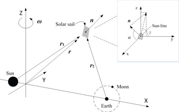
The frame of reference rotating with angular velocity
 ${\omega}$
is established where the Sun, the Earth-Moon system and the sail consist of the CR3BP model, shown as Figure 1. The origin is taken at the barycenter of the Sun and Earth-moon system; the X axis goes from the Sun to the Earth-Moon barycenter; the Z axis is the axis of rotation, and the Y axis completes the triad.
Solar sail circular restricted three-body problem.

To simplify, the sum of the two primary masses, period of primary masses around their barycenter and distance between the primary masses are all taken to be dimensionless units, so that the angular velocity of the rotating reference frame is defined as
 ${\omega} =1$
. Then the dynamics of the sail are characterised by the system's mass ratio defined as
 $\mu =m_{2}/\break \lpar m_{1}+m_{2}\rpar $
, where m
1 denotes the Sun's mass and m
2 denotes the Earth-Moon system mass. The sail position vectors are defined with respect to the origin as
 ${{r}} = \lpar x\comma \; y\comma \; z\rpar $
, to the Sun as
 ${{r}}_{1} = \lpar x+\mu\comma \; y\comma \; z\rpar $
, to the Earth-Moon barycenter as
 ${{r}}_{2} = \lpar x-1+\mu\comma \; y\comma \; z\rpar $
, to the Earth as
 ${{r}}_{e}= \lpar x-x_{e}\comma \; y-y_{e}\comma \; z-z_{e}\rpar $
and to the Moon as
 ${{r}}_{m}= \lpar x-x_{m}\comma \; y-y_{m}\comma \; z-z_{m}\rpar $
where
 $\lpar x_{e}\comma \; y_{e}\comma \; z_{e}\rpar $
and
 $\lpar x_{m}\comma \; y_{m}\comma \; z_{m}\rpar $
are respectively the coordinates of the Earth and the Moon.
Then the vector equation of a sail in the rotating frame can be written as
 $$\ddot{{{r}}}+2{\omega} \times \dot{{{r}}}+\nabla U={{a}}$$
where the three-body potential U and the solar radiation pressure acceleration
 ${{a}}$
are defined as
 $$U=-\left[{1 \over 2}(x^2+y^2)+{1-\mu \over r_{1}}+{\mu \over r_{2}}\right]$$
 $${{a}}=\beta {(1-\mu) \over r_{1}^2}(\hat{{{r}}}_{1} \cdot {{n}})^2{{n}}$$
where β is the solar sail lightness number, defined as the magnitude ratio of the solar radiation over the gravity pressure, and n is the normal vector of the sail whose direction is opposite to the Sun.
 $\ddot{{{r}}}=\dot{{{r}}}=0$
can be used to derive the equation generating ALP as
 $${{a}}=\nabla U.$$
Since
 ${{a}}$
is oriented in direction
n
, then taking the vector product of
n
with Equation (1), it follows that
 $$\nabla {{U}}\times {{n}}={0}, \mid {{n}} \mid={{1}} \Rightarrow {{n}}={\nabla {{U}} \over \mid {\nabla {{U}}}\mid}.$$
Thus, the solar sail lightness number required can also be obtained as
 $$\beta ={r_{1}^2 \over 1-\mu }{\nabla {{U}}\cdot {{n}} \over (\hat{{{r}}}_{1}\cdot {{n}})^2}.$$
The solar sail attitude and lightness number required for the artificial equilibria have been obtained above. Since n and β can be chosen in accordance with Equations (5) and (6), the classical five Lagrangian points will be replaced by an infinite set of new artificial equilibrium solutions.
2.2. Regions of Artificial Equilibrium Solutions
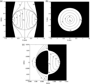
As the solar radiation pressure force can never be directed sunward, the sail attitude is constrained physically so that the regions of artificial equilibrium solutions are defined by
 $$({{r}}_{1} \cdot \nabla {{U}})\ge 0$$
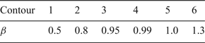
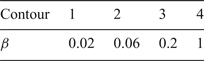
and demonstrated in Figure 2. All of the five classical equilibria lie on the boundary of regions because they are solutions to
 $\nabla {{U}}={0}$
. As can be seen from Figure 2(c), near m
2, there are two topologically disconnected surfaces S1 and S2 which define the boundary to the region. The outer surface S1 excludes solutions along the X-axis from
 $-\infty <x<x_{L_{3}}$
and
 $x_{L_{2}} <x<\infty $
while the inner surface S2 excludes solutions along the X-axis from
 $x_{L_{1}} <x<1-\mu $
, where
 $x_{L_{1}}$
,
 $x_{L_{2}}$
and
 $x_{L_{3}}$
respectively denote the x coordinate component of the collinear Lagrangian points L
1, L
2 and L
3.

Solar sail lightness number.

Solar sail lightness number near.

As demonstrated above, the surfaces of constant lightness number increase with approaching the surfaces asymptotically. It is clear from Equation (6) that in the limit as
 ${{r}}_{1} \cdot \nabla {{U}}\to {0}$
,
 $\beta \to \infty $
.
3. CANDIDATE ARCHITECTURE OF NAVIGATION CONSTELLATION
Based on the fact that the deployment and folding process of the sail membrane are very complicated, sail lightness number just allows for small variations due to the limitation of industrial manufacture. Therefore, a two-layer optimisation strategy including the navigation constellation distribution and sail's trajectory design is developed to respectively minimise the required lightness number at ALP (β ) and the lightness number's variation as the sail moves around the ALP (Δ β).
For the first-layer optimisation, ALPs of the Sun-Earth system are chosen to construct the basic navigation constellation architecture, and the selected ALPs are referred to later as the candidate ALPs. Considering the navigation accuracy, the candidate ALPs should be more dispersed and relatively evenly distributed. Herein, a group of four candidate ALPs in a configuration of a regular tetrahedron shape is adopted.
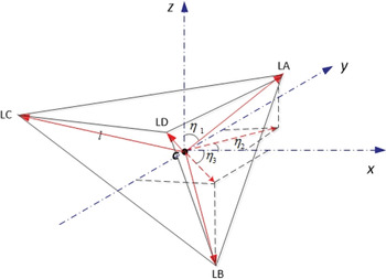
Because of the symmetry about y and z components in artificial equilibria regions, the centre of the regular tetrahedron, denoted by C is arranged in the X axis, and the four vertices of the tetrahedron are respectively denoted by LA, LB, LC and LD. The size of the tetrahedron is characterised by the distance l between its centre and vertex; and the orientation is characterised by the distance d from m
2 to C and three angles which are now defined: η1 is the angle from Z axis to the vector
 ${{r}}_{CLA}$
, η2 is the angle from X axis to the projection of vector
 ${{r}}_{CLA}$
in the X-Y plane, and η3 is the angle from X axis to the projection of vector
 ${{r}}_{CLB}$
in the X-Y plane, shown in Figure 3.
Schematic of the regular tetrahedron's size and orientation.

The position of candidate ALPs can be uniquely identified by the column vector
 $\lpar \eta_{1}\comma \; \eta_{2}\comma \; \eta_{3}\comma \; l\comma \; d\rpar $
, and the relations between them are derived as follows:
 $$\eqalign {& \left[\matrix{x \cr y \cr z }\right]_{LA} = \left[\matrix{l\sin (\eta _1)\cos (\eta _2) \cr l\sin (\eta _1)\sin (\eta _2) \cr l\cos (\eta _1)\quad \quad \quad \cr} \right]+ C_1; \cr & \left[\matrix{x \cr y \cr z } \right]_{LB} = \left[ \matrix{ 4l/3 \sqrt 2 \cdot \cos (\eta _3) \cr 4l/3 \sqrt 2 \cdot \sin (\eta _3) \cr 0 \quad \quad \quad\quad\quad\quad \cr} \right] \cdot R_1^{ - 1} \cdot R_2^{ - 1} + C_2 + C_1 \cr & \left[\matrix{ x \cr y \cr z } \right]_{LC} = \left[\matrix{4l/3 \sqrt 2 \cdot \cos (\eta _3 + 120^\circ)\cr 4l/3 \sqrt 2 \cdot \sin (\eta _3 + 120^\circ)\cr 0 \quad \quad \quad \quad \quad \quad\quad\quad\quad \cr}\right] \cdot R_1^{ - 1} \cdot R_2^{ - 1} + C_2 + C_1; \cr & \left[\matrix{x \cr y \cr z }\right]_{LD} = \left[\matrix{4l/3 \sqrt 2 \cdot \cos (\eta _3 + 240^\circ) \cr 4l/3 \sqrt 2 \cdot \sin (\eta _3 + 240^\circ) \cr 0 \quad \quad \quad \quad \quad \quad\quad\quad\quad\cr} \right] \cdot R_1^{ - 1} \cdot R_2^{ - 1} + C_2 + C_1}$$
where
 $$C_1 =\left[\matrix{1-\mu +d \cr 0 \quad \quad \quad \cr 0 \quad\quad\quad \cr}\right] \quad C_2 =\left[\matrix{-l/3\sin\,( {\eta_1 })\cos\,( {\eta_2 }) \cr -l/3\sin\,( {\eta_1 })\sin\,( {\eta_2 }) \cr -l/3\cos\,( {\eta_1 }) \quad\quad\quad \cr}\right]$$
 $$ R_1 =\left[\matrix{\cos\,( {-\eta_1 }) & 0 & -\sin\,( {-\eta_1 }) \cr 0 & 1 & 0 \cr \sin\,( {-\eta_1 }) & 0 & \cos\,( {-\eta_1 })} \right] \quad R_2 =\left[\matrix{{\cos\,( {-\eta_2 })} & {\sin\,( {-\eta_2 })} & 0 \cr {-\sin\,( {-\eta_2 })} & {\cos\,({-\eta_2 })} & 0 \cr 0 & 0 & 1 } \right]$$
Then the variables
 $\eta_{1}\comma \; \eta_{2}\comma \; \eta_{3}\comma \; l\comma \; d$
are taken as design variables to attain the optimisation of the objective function
 $\bar {\beta }$
, which is defined as the average lightness number of the four ALPs. The optimisation problem is formularised as
 $$\min \bar {\beta }(\eta_1 ,\eta_2 ,\eta_3 ,d,l)={\beta_{LA} +\beta_{LB} +\beta_{LC} +\beta_{LD} \over 4}$$
subject to:
 $$\left\{ \matrix{ -( {{r}_{1} \cdot \nabla {U}} )\le 0 \hfill \cr -90^\circ \le \eta_1 \le 90^\circ \hfill \cr -90^\circ \le \eta_2 \le 90^\circ \hfill \cr -90^\circ \le \eta_3 \le 90^\circ \hfill \cr -0.01\le d\le 0.01 \hfill \cr 0\lt l\le 0.02 \hfill \cr} \right.$$
where β
i
denotes the desired lightness number at the ALPi,
 $i\in \lpar {LA}\comma \; {LB}\comma \; {LC}\comma \; {LD}\rpar $
.
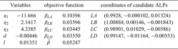
Optimisation for the objective function is implemented with the constrained nonlinear multi-variable function “fmincon” in MATLAB, which attempts to find a constrained minimum of a scalar function of several variables starting at an initial estimate (initial estimate of variable vector in this paper is set as (−20; 50; 25; −0.006; 0.008)). A group of the optimal solutions is solved and the coordinates of candidate ALPs are obtained according to Equation (8), shown in Table 3.
Optimal solution of the regular tetrahedron configuration and coordinates of candidate ALPs.

Equation (6) shows β required at the ALP also has symmetry about the y and z components, thus another three groups of candidate ALPs which are XY-plane symmetric with LA, LB, LC and LD (referred as
 ${LA}^{(1)}$
,
 ${LB}^{(1)}$
,
 ${LC}^{(1)}$
and
 ${LD}^{(1)}$
) or XZ-plane symmetric ( referred as LA
(2),
 ${LB}^{(2)}$
,
 ${LC}^{(2)}$
and
 ${LD}^{(2)}$
) or X-axis symmetric (referred as
 ${LA}^{(3)}$
,
 ${LB}^{(3)}$
,
 ${LC}^{(3)}$
and
 ${LD}^{(3)}$
) must share the same
 $\bar {\beta}$
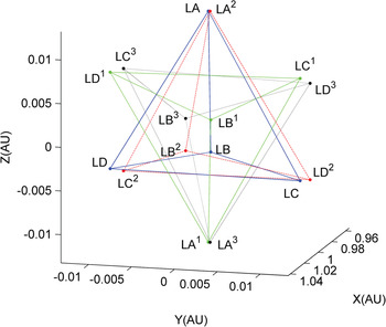
with the group of ALPs in Table 3. The position of the four groups' candidate ALPs in the rotating frame is demonstrated in Figure 4. Importantly, in order to achieve a better navigation performance, it is recommended to increase the coverage of the navigation constellation and all these four groups' candidate ALPs participate in the navigation architecture. That is to say, the trajectory design in Section 4 should be implemented to the total 16 candidate ALPs to make preparation for the evaluation of navigation performance in Section 5.
Distribution of the four groups' candidate ALPs: blue solid line is the first regular tetrahedron, green dash line is the XY-plane symmetric tetrahedron, red dash-dot line is the XZ-plane symmetric tetrahedron, and black dot line is the X-axis symmetric tetrahedron.

4. TRAJECTORY DESIGN FOR NAVIGATED SOLAR SAIL
4.1. Dynamics of Solar Sail Moving around ALP
Considering the perturbation from the Moon, the solar sail is no longer stationary at the ALP. To keep the sail moving in a bounded periodic or quasi-periodic trajectory near the artificial equilibrium
 ${{r}}_{0}$
, an extra control provided by changing attitude angles and lightness number is used. Then the sail's controlled equation around the ALP denoted as
 ${{r}}_{0}$
is derived as
 $${d^2{{r}} \over dt^2}+2{\omega} \times {d{{r}} \over dt} +\nabla U_f ({{r}})={{a}}({{r}},{\Theta} )$$
where
 ${\Theta} =\lsqb \alpha \comma \; \gamma \comma \; \beta \rsqb ^{\rm T}$
are the sail's parameters including the attitude angles α and γ and the lightness number β, the position vector of sail
r
has the deviation
 ${\delta}$
with respect to
 ${{r}}_{0}$
, i.e.,
 ${{r}}={{r}}_{0}+{\delta}$
, and U
f
is the four-body potential function, shown as
 $$U_f =-\left[ {{1 \over 2}(x^2+y^2)+{1-\mu \over r_{1}}+{m_e \over r_e }+{m_m \over r_m}} \right]$$
where m
e
and m
m
are respectively the dimensionless mass of the Earth and Moon which satisfy m
e
(+)m
m
(=)μ. For the controlled sail, the parameters
 ${\Theta}$
can be expressed as
 ${\Theta} ={\Theta}_{0} +\Delta{\Theta} $
, where
 ${\Theta}_{0} $
represents the attitude angles and lightness number to stop the sail at
 ${{r}}_{0}$
, and
 $\Delta{\Theta}$
is the extra variation of parameters to provide the required control acceleration for bounded trajectory around the ALP.
Then, the solar radiation pressure acceleration can be expanded in a Taylor series about the equilibrium solution as
 $$\eqalign{&{a}({r}_0 +{\delta},{\Theta}_0 +\Delta{\Theta}) ={a}({r}_0,{\Theta}_0)+ \left. {{\partial {a}({r},{\Theta}) \over \partial {r}}} \right \vert_{{{r}={r}_0 \atop {\Theta} ={\Theta}_0}} {\delta} +\left.{\partial {a}({r}, {\Theta} ) \over \partial {\Theta}}\right\vert_{{{r}={r}_0 \atop {\Theta} ={\Theta}_0}} \cr & \quad \times \Delta{\Theta} + \hbox{O}\lpar {\vert {\delta}\vert^2}\rpar +\hbox{O}\lpar {\vert {\Delta{\Theta} }\vert^2}).}$$
where
 ${\partial {{a}}\lpar {{r}}\comma \; {\Theta} \rpar \over \partial {{r}}}$
and
 ${\partial {{a}}\lpar {{r}}\comma \; {\Theta} \rpar \over \partial {\Theta} }$
are respectively the derivative matrices of the solar radiation pressure acceleration to the position vector
r
and the sail's parameter
 ${\Theta}$
, given by Equation (16) and Equation (22).
 $${\partial {{a}}({{r}},{\Theta} ) \over \partial {{r}}}={\beta} \lpar {1-\mu } \rpar \cos \alpha ^2{{n}}\left[{2(x+\mu )\over r_1^4 } \,\,\,\, {2y \over r_1^4 } \,\,\,\, {2z \over r_1^4 } \right]$$
Neglecting the second order small quantity, substitute Equation (15) into Equation (13) to yield the relative equation around ALP as
 $$\ddot{{\delta} }+{{M}}_0 \dot{{\delta}}+{{M}}_1 {\delta}={{M}}_2 +{{T}}_c$$
where
 $$\eqalign{&{M}_0 = \left[\matrix{0 & -2 & 0 \cr 2 & 0 & 0 \cr 0 & 0 & 0 }\right], \quad {M}_1 =-\left. {\partial {a}({r},{\Theta} ) \over \partial {r}} \right\vert_{r=r_0 \atop \Theta =\Theta_0}, \cr & M_2 =\nabla U(r_0)-\nabla U_f (r),\quad T_c =\left. {\partial a(r, \Theta) \over \partial \Theta } \right\vert_{r=r_0 \atop \Theta =\Theta_0} \Delta{\Theta}.}$$
The control acceleration is denoted by
 ${{T}}_{c}$
which is achieved by regulating the sail's parameters. For the second-layer optimisation, the bounded quasi-periodic trajectory with minimum lightness number control is designed. Firstly, the powerful Hamiltonian structure-preserving controller developed in Xu and Xu (Reference Xu and Xu2009) is followed to guarantee the boundedness of trajectory; then, the differential evolution algorithm is adopted to select the optimal trajectory with the minimum Δ β.
4.2. Trajectory Optimisation with Differential Evolution Algorithm
According to Howell (Reference Howell2001), the CR3BP is classified as the hyperbolic Hamiltonian system, in which the three Degree-Of-Freedom (3-DOF) hyperbolic equilibria have one-dimensional stable manifolds, one-dimensional unstable manifolds, and four-dimensional centre manifolds. Referring to Xu and Xu (Reference Xu and Xu2009), the Hamiltonian Structure-Preserving controller (HSP) they developed can stabilise the system by only position feedback and generate quasi-periodic and Lyapunov stable trajectories. The four kinds of manifolds' gains for feedback are represented by G 1, G 2, G 3, and G 4 respectively, and the controller is constructed as
 $${{T}}_c =[ {-\sigma^2(G_1 {{u}}_+ {{u}}_+^T +G_2 {{u}}_- {{u}}_-^T )-\vartheta^2G_3 ({{uu}}^H+\bar {{{u}}}\bar {{{u}}}^H)-\xi^2G_4 ({{vv}}^H+\bar {{{v}}}\bar {{{v}}}^H)} ] {\delta}$$
where
 ${{u}}_+ $
and
 ${{u}}_- $
are the stable and unstable manifolds of the hyperbolic eigenvalues ±σ,
 ${{u}}$
and
 $\bar{{{u}}}$
are the centre manifolds of elliptic eigenvalues
 $\pm i\vartheta $
,
 ${{v}}$
and
 $\bar{{{v}}}$
are the centre manifolds of the other elliptic eigenvalues ±iξ, and
 ${\delta}$
is the position feedback to the equilibrium
 ${{r}}_{0}$
. The formula to compute the manifolds and eigenvalues above can be found in Koon et al. (Reference Koon, Lo, Marsden and Ross2000).
For the 3-DOF sail, the HSP controller
 ${{T}}_{c}$
is achieved by changing
 ${\Theta} =\lsqb \alpha \comma \; \gamma \comma \; \beta \rsqb ^{T}$
. The values of
 ${\Theta}$
should be estimated by the allocation law of
 ${{T}}_{c}$
to check if the controller can be implemented in the mechanism or not. The attitude angle α is defined as the angle from the Sun-line to
n
and the attitude angle γ is defined as the angle from y axis to the projection of
n
in the y-z plane. From the definition of α and γ, the sail's normal vector
n
can be formularised as
 $$n=\left[ \matrix{n_x \cr n_y \cr n_z } \right]=\left[\matrix{\cos \alpha \cos \theta_1 \cos \theta_2 -\sin\alpha\cos\gamma \sin\theta_2 -\sin\alpha \sin \gamma\sin \theta_1 \cos \theta_2 \cr \cos \alpha \cos \theta_1 \sin \theta_2 +\sin\alpha\cos\gamma \cos\theta_2 -\sin\alpha \sin \gamma\sin \theta_1 \sin \theta_2 \cr \cos \alpha \sin \theta_1 +\sin\alpha \sin \gamma \cos \theta_1 } \right]$$
where θ1 is the angle from X-Y plane to
 ${{r}}_{1}$
and θ2 is the angle from [1 0 0]
T
to the projection of
 ${{r}}_{1}$
in the X-Y plane.
Then, the controller's allocation law is addressed by the first-order estimated values of
 ${\Theta}$
as
 $$\Delta{\Theta} = \left.\left[{\partial {{a}} \over \partial {\Theta}}\right]^{-1}\right \vert_{{{r}}_0} \cdot {{T}}_c,$$
where
 $${\partial a \over \partial \Theta} =\left[{\partial a \over \partial \alpha} \,\, {\partial a \over \partial \gamma} \,\,{\partial a \over \partial \beta}\right]=\left[ \matrix{{\partial a_x \over \partial \alpha} & {\partial a_x \over \partial \gamma } & {\partial {a}_x \over \partial \beta } \cr {\partial {a}_y \over \partial \alpha } & {\partial {a}_y\over \partial \gamma } & {\partial {a}_y \over \partial \beta } \cr {\partial {a}_z \over \partial \alpha } & {\partial {a}_z \over \partial \gamma } & {\partial {a}_z \over \partial \beta }} \right] $$
 $$ \eqalign{{\partial a_x \over \partial \alpha } & ={\beta (1-\mu )\cos \alpha \over r_1^2} \cr & \times \left[ {{-3( {x+\mu })\sin \alpha \cos \alpha \over \mid{r_1}\mid}-{(1-3\sin^2\alpha ) \over \sqrt {({x+\mu})^2+y^2}} \left( {y\cos \gamma -{({x+\mu})z\sin\gamma \over \mid{r_1}\mid}} \right)} \right]; \cr {\partial a_y \over \partial \alpha }&= {\beta (1-\mu )\cos \alpha \over r_1^2 }\left[ {{-3y\sin \alpha \cos \alpha \over \mid{r_1}\mid} +{(1-3\sin^2\alpha ) \over \sqrt {\lpar {x+\mu } \rpar^2+y^2}} \left( {( {x+\mu })\cos \gamma -{yz\sin \gamma \over \mid{r_1}\mid}} \right)} \right]; \cr & \quad \quad {\partial a_z \over \partial \alpha } ={\beta (1-\mu )\cos \alpha \over r_1^2 }{-3z\sin \alpha \cos \alpha +(1-3\sin ^2\alpha )\sin \gamma \sqrt {( {x+\mu })^2+y^2} \over \mid{r_1 }\mid}; \cr & \quad \quad\quad\quad {\partial a_x \over \partial \gamma } ={\beta (1-\mu )\cos ^2\alpha \over r_1^2 }{\sin \alpha \over \sqrt {({x+\mu })^2+y^2} } \left[{y\sin \gamma -{( {x+\mu })z\cos \gamma \over \mid {r_1 }\mid}} \right]; \cr & \quad \quad\quad\quad {\partial a_y \over \partial \gamma } = {\beta (1-\mu )\cos ^2\alpha \over r_1^2 }{\sin \alpha \over \sqrt {({x+\mu })^2+y^2} } \left[{-( {x+\mu })\sin \gamma -{yz\cos \gamma \over \mid {r_1 } \mid}} \right]; \cr & \quad \quad\quad\quad {\partial a_z \over \partial \gamma } ={\beta (1-\mu )\cos ^2\alpha \over r_1^2 }{\sin \alpha \cos \gamma \sqrt {( {x+\mu })^2+y^2} \over \mid {r_1 } \mid} \cr & \quad \quad\quad\quad\quad\quad\quad\quad\quad\quad\quad\quad {\partial a_x \over \partial \beta } ={(1-\mu )\cos ^2\alpha \over r_1^2}\cdot n_x \cr & \quad \quad\quad\quad\quad\quad\quad\quad\quad\quad\quad\quad {\partial a_y \over \partial \beta }={(1-\mu )\cos ^2\alpha \over r_1^2}\cdot n_y \cr & \quad \quad\quad\quad\quad\quad\quad\quad\quad\quad\quad\quad {\partial a_z \over \partial \beta } ={(1-\mu )\cos ^2\alpha \over r_1^2}\cdot n_z} $$
It is expected that with the controller and appropriate initial state, the bounded quasi-periodic trajectory can be generated around the sail equilibrium point
r
0, and the time histories of
 $\Delta {\Theta}$
can be obtained as well.
To search for the simple and useful approach to propagate the trajectory of libration points, this paper presents a trajectory design based on an optimisation algorithm. The six-dimensional initial estimation of trajectory and four manifolds' controller gains work as the design variables to optimise the new objective function which is defined to measure the lightness number variation. Considering the number of design variables, a Differential Evolution (DE) algorithm (Qin et al., Reference Qin, Huang and Suganthan2009) which is inspired by the natural evolution of species, is adopted as an efficient and powerful population-based stochastic search technique to solve this optimisation problem.
The population size in the DE algorithm is set as 15, and the maximum generation is set as 50. An optimisation task is characterised by the mean square error of Δ β as
 $$\min F({{G}},\delta {{r}}_0,\delta \dot{{{r}}}_0)=V(\Delta \beta )$$
where
 ${{G}}=\lsqb G_{1}\comma \; G_{2}\comma \; G_{3}\comma \; G_{4}\rsqb ^{T}$
,
 $\delta {{r}}_{0}$
and
 $\delta \dot{{{r}}}_{0} $
are respectively the initial position estimation and initial velocity estimation of equilibrium
 ${{r}}_{0}$
and V is the mean square error. The specific process to compute F is demonstrated in Figure 5, where the DE algorithm aims at evolving a population of 15 ten-dimensional parameter vectors towards the global optimum. For every generation, the sail's trajectory can be propagated by Equation (17) and
 $\Delta {\Theta}$
can be calculated with the allocation law, then the optimal solution for minimum objective function can be obtained by comparison and selection.
Flowchart to compute the objective function F of the navigated sail.

4.3. Simulations of the Resulting Orbits
According to the conclusion in Section 3, the four groups' candidate ALPs with the same
 $\bar {\beta }$
are implemented with trajectory optimisation to obtain the motion of navigated solar sails. Herein an instance of candidate LC, i.e.,
 ${{r}}_{0} =\lsqb 0.98901\comma \; 0.01029\comma \; -0.00586\rsqb ^{T}$
is presented with the designed trajectory and time histories of
 $\Delta {\Theta}$
. The ten-dimensional parameter vector is optimised via the DE algorithm as
 $$\left\{\matrix{ G=[46.623,29.079, 62.059,54.676] \cr \delta {{r}}_0 =[-2.4157,9.3566,5.7759]\cdot 10^{-6} \cr \delta \dot{{{r}}}_0 =[-3.2741,-2.943,4.223]\cdot 10^{-6} } \right.$$
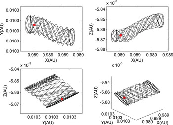
The trajectory of solar sail near the equilibrium LC generated by the optimised initial state and the dynamical model Equation (17) is demonstrated in Figure 6. The time histories of
 $\Delta {\Theta} $
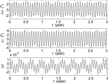
required by the HSP controller for quasi-periodic trajectory near LC are shown in Figure 7.
 $\Delta \alpha $
ranges from −2.639 to 2.985,
 $\Delta \gamma $
is from −3.69 to 4.192, and Δ β is just from −0.00255 to 0.0013. Thus the slight variation of lightness number absolutely guarantees the implementation of HSP controller for trajectory design near LC in the mechanism.
Quasi-periodic trajectory of sail near the candidate ALP LC: red dot represents the point LC.

Δ Θ for the quasi-periodic trajectory of sail near the equilibrium LC.

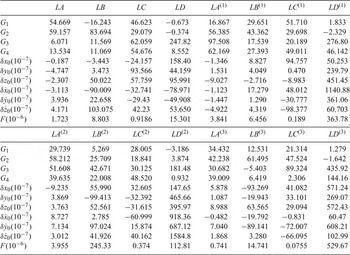
The same approach can be applied to the quasi-periodic trajectory design of sail near another fifteen candidate ALPs. The optimisation results of the initial estimation and four manifolds' gains as well as the mean square error of Δ β are summarised in Table 4, with which all the sails' bounded quasi-periodic trajectories can be propagated. It is indicated from Table 4 that the maximum mean square error of Δ β is
 $5.2967\times 10^{-4}$
, which greatly reduces the requirements for the sail's equipment and is small enough to be easily accepted in the mechanism. Thus the feasibility of the sail constellation configuration from the aspect of implementation in practice is validated.
Optimisation results of navigated solar sails' trajectory.

where F is defined as the mean square error of Δ β,
 $F=V\lpar \Delta \beta\rpar $
.
5. NAVIGATION PERFORMANCE ANALYSIS
5.1. Geometric Dilution of Precision (GDOP)
GDOP is a ratio of pseudo-range measurement error to user's location error and relates closely to the constellation distribution. Since it is irrelevant to the selected coordinate system, GDOP becomes the main basis for solar sail selection and directly contributes to the navigation accuracy. The formula to calculate GDOP is (Yang et al., Reference Yang, Li, Xu and Tang2011):
 $$\hbox{GDOP}=\sqrt {tr({{E}}^T{{E}})^{-1}}$$
where tr is the trace of the matrix
 $\lpar {{E}}^{T}{{E}}\rpar ^{-1}$
shown as
 $$({{E}}^T{{E}})^{-1}= {{{E}}^\ast \cdot {{E}}^{T\ast} \over \vert{{E}}\vert^2} ={{{E}}^\ast\cdot {{E}}^{T\ast} \over 36Vol^2}$$
Thus, GDOP can be derived as
 $$\hbox{GDOP}={\sqrt {tr({{E}}^\ast \cdot {{E}}^{T\ast})} \over 6Vol}$$
where E is a coefficient matrix, composed of the direction cosine of the position vector from user to four candidate ALPs, * represents the adjoint matrix, Vol represents the volume of the tetrahedron. It is shown from Equation (27) that GDOP is inversely proportional to the volume of the tetrahedron. When the tetrahedron is regular, it attains its maximum volume and the GDOP is at a minimum. Based on this fact, the regular tetrahedron adopted as the constellation geometric configuration in this paper has better position accuracy.
In general, users can achieve positioning with signals from four sails simultaneously. Therefore, to minimise the location error, a method referred to as optimal GDOP factor is implemented as the algorithm to select four sails with the best relative geometry positions. In every certain interval of time, make permutations and combinations of four sails from all the arranged solar sails successively, and then compute the corresponding value of GDOP. The sails combination with minimum GDOP is selected for the positioning calculation.
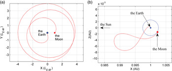
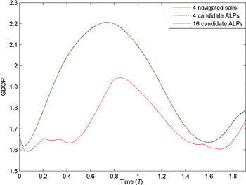
The traditional approach to construct a spacecraft transfer trajectory to the Moon from the Earth is by the well-known Hohmann transfer (Prussing, Reference Prussing1992), which is constructed by determining a two-body Keplerian ellipse from an Earth parking orbit to the orbit of the moon (Koon et al., Reference Koon, Lo, Marsden and Ross2001). However, as the Hohmann transfer requires a large change in velocity for the spacecraft to be captured into an elliptic orbit about the moon, an innovative trajectory design named Weak Stability Boundary (WSB) transfer was introduced by Belbruno (Reference Belbruno1987) to use a low energy transfer with a ballistic capture at the Moon, which requires less fuel than the usual Hohmann transfer but longer flight time. With the advantages of WSB transfer method over classical approaches, the WSB transfer was subsequently applied to the rescue of the Japanese mission Hiten (Belbruno, Reference Belbruno2004) and the trajectory design of the Grail spacecraft at NASA (Edwards-Stewart, Reference Edwards-Stewart2003). Due to the great research value and wide application of the low-energy transfer method (Zhang et al., Reference Zhang, Zhao and Zhang2015; Zhao et al., Reference Zhao, Gurfil and Zhang2016), the trans-lunar weak stability boundary low energy trajectory is taken as an example to evaluate the navigation performance of the solar sail constellation. A developed numerical algorithm in Peng and Xu (Reference Peng and Xu2015) is used in this paper to create a nominal WSB trajectory, demonstrated in Figure 8, and the GDOP of such a cislunar trajectory is shown in Figure 9 with the method of the optimal GDOP factor.
Trans-lunar WSB low energy trajectory: a) trajectory in Earth-Moon rotating reference frame; b) trajectory in Sun-Earth+Moon rotating reference frame; red line represents the WSB low energy trajectory, and blue line represents the orbit of the Moon around the Earth.

GDOP of the trans-lunar WSB low energy trajectory: T is the orbital period of the Sun-Earth+Moon system revolving around their barycenter; green solid line denotes the GDOP of constellation by navigated sails around LA, LB, LC, LD; black dash line denotes the GDOP of constellation by candidate ALPs LA, LB, LC, LD; red solid line denotes the GDOP obtained with the optimal GDOP factor from sixteen candidate ALPs.

It is indicated that as the navigated sail moves in a much smaller neighbourhood of the candidate ALP, the GDOP of the constellation by navigated sails (green solid line) and constellation by candidate ALPs (black dash line) are nearly the same. Thus we simply take the optimal GDOP of the navigation constellation by 16 candidate ALPs to represent the navigation performance of this solar sail navigation constellation. Besides, Figure 9 also shows that the GDOP of the WSB low energy trajectory changes with time relatively smoothly, ranging from 1.594 to 1.939 without an obvious jump. It is expected that the constellation of 16 navigated sails has the lower average GDOP, calculated as 1.717. Compared with the Global Positioning System (GPS), whose users mostly fly in low earth orbit and the corresponding GDOP ranges from 2 to 6 (Doong, Reference Doong2009), navigation constellation by displaced sail can navigate users in cislunar orbit with a certain accuracy.
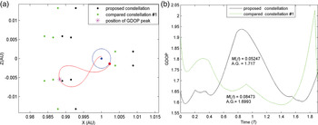
To qualify the work, more discussion on the peak in GDOP is presented, whose position corresponds to the purple point labelled by ‘*’ in the WSB trajectory of Figure 10(a), referred to as P* later. This shows that P* is outside the proposed constellation configuration (black points), so the coverage efficiency for P* is decreasing and the value of GDOP becomes relatively large. Then a new constellation configuration which covers P* is designed by deviating the proposed constellation leftwards in the X axis direction (green points in Figure 10(a)), to investigate if it can obtain a lower GDOP for P* and even the whole trajectory. The two groups of GDOP are demonstrated in Figure 10(b) for GDOP and average lightness number comparison.
Comparison between two constellations: (a) projection of two navigation constellations in the X-Z plane, where the purple point is the position of GDOP peak, referred to as P*; (b) GDOP of the two different navigation constellations to the same WSB trajectory, where A.G. represents average GDOP.

Simulation results in Figure 10(b) indicate that the compared constellation #1 indeed decreases the GDOP at P* but meanwhile sharply increases the GDOP of trajectory near the Earth (shown as the jump in the green line), which results from the increasing distance between 12 candidate ALPs on the left of the Earth and the trajectory in the cislunar space. Compared to constellation #1, the proposed navigation constellation shows the advantages of relatively smooth GDOP and more accurate navigation for a WSB trajectory on the Earth's right. In addition to the WSB trajectory transiting LL1
point simulated in this paper, it is also expected that the proposed navigation constellation can have a low GDOP and high accuracy for the WSB trajectory transiting LL2
point (Zeng and Zhang, Reference Zeng and Zhang2016). Furthermore, constellation #1 decreases the average GDOP from 1.717 to 1.699 at the cost of increasing
 $\bar {\beta }$
from 0.05247 to 0.08473, which places a higher demand on the sail manufacturing. In conclusion, the GDOP of the proposed navigation constellation system by displaced solar sail presents a good performance in cislunar space navigation while promising sufficient feasibility of lightness number in the mechanism.
5.2. Filter Algorithm to Evaluate the Navigation Performance
Focusing on the navigation constellation construction and feasibility study of navigation, this paper adopts the classical Extended Kalman Filter (EKF) algorithm rather than developing a new algorithm to verify the navigation performance. The EKF algorithm is the optimal estimation technique used in real-time navigation to estimate errors of the system states with the measurement output, and then to correct the system with such estimation. The state vector being estimated consists of the position and velocity of the spacecraft as
 $${{X}}=[ x\ y\ z\ v_x\ v_y\ v_z ]^T$$
which is governed by a system of nonlinear differential equations, denoted by
 $$\dot{{{X}}}={{f}}({{X}},t)+{{W}}\,(t)$$
where f ( X , t) is the nonlinear dynamic model function, W (t) is a sequence of zero-mean, white, Gaussian process noise.
The discretised filtering model used in the EKF is
 $$\eqalign{&{X}_k={\Phi}\,(t_{k},t_{k-1})\,{X}_{k-1} +{W}_{k-1} \cr & Z_k =H_k X_k +N_k}$$
where
 ${{Z}}$
is the measurement vector,
 $\bi{\Phi}$
is the state transition matrix,
H
is the measurement matrix and
N
is the measurement noise.
As a real time recursive data processing approach, the Kalman filter can take the state estimation
 $\bar{{{X}}}_{k-1}$
at last time t
k−1 and measurement vector
 ${{Z}}_{k}$
at time t
k
to attain the state prediction
 ${{X}}_{k}^{\ast} $
at time t
k
, then further obtain the state estimation
 $\bar{{{X}}}_{k} $
at the current time t
k
. The modified covariance propagation formula from time t
k−1 to time t
k
can be obtained with the state transition matrix
 $\bi{\Phi}$
(Montenbruck and Gill, Reference Montenbruck and Gill2000):
 $$p_{k \mid k-1} ={\bi{\Phi}} (t_k ,t_{k-1} )p_{k-1} {\bi{\Phi}}^T(t_k ,t_{k-1}) + \int_{t_{k - 1}}^{t_k} {{\bi{\Phi}} (t_k ,\tau )} {{Q}}(\tau ){\bi{\Phi}}^T(t_k,\tau )d\tau$$
where
Q
is the process noise covariance matrix which is a diagonal matrix, and the state transition matrix
 ${\bi{\Phi}}$
can be determined by integrating a differential equation related to the Jacobian of the dynamic model function
f
, i.e.,
 $$\eqalign {& {\bi{\dot\Phi}}(t,t_k ) = {A}(t){\bi{\Phi}} (t,t_k ) \cr & \quad {A}(t) = {\partial f(X^\ast ,t) \over \partial {X}(t)}}$$
A measurement update for the state and covariance matrix can then be computed with the classical EKF algorithm (Zhang and Xu, Reference Zhang and Xu2014), where the measurement matrix
 ${{H}}_{k}$
with elements for the observational sail-to-spacecraft range data is computed using the current state as
 $${H}_k ={\partial \rho ({X}^\ast ,t_k ) \over \partial {X}}=\left[\matrix{\displaystyle{x_k^\ast -x_{1^\ast } \over \rho_{k1^\ast } } & \displaystyle{{y_k^\ast -y_{1^\ast } \over \rho_{k1^\ast } }} & \displaystyle{{z_k^\ast -z_{1^\ast } \over \rho_{k1^\ast }}} & 0 & 0 & 0 \cr \displaystyle{{x_k^\ast -x_{2^\ast } \over \rho_{k2^\ast } }} & \displaystyle{{y_k^\ast -y_{2^\ast } \over \rho_{k2^\ast } }} & \displaystyle{{z_k^\ast -z_{2^\ast } \over \rho_{k2^\ast } }} & 0 & 0 & 0 \cr \displaystyle{{x_k^\ast -x_{3^\ast } \over \rho_{k3^\ast } }} & \displaystyle{{y_k^\ast -y_{3^\ast } \over \rho_{k3^\ast } }} & \displaystyle{{z_k^\ast -z_{3^\ast } \over \rho_{k3^\ast } }} & 0 & 0 & 0 \cr \displaystyle{{x_k -x_{4^\ast } \over \rho_{k4^\ast } }} & \displaystyle{{y_k-y_{4^\ast } \over \rho_{k4^\ast } }} & \displaystyle{{z_k -z_{4^\ast } \over \rho_{k4^\ast } }} & 0 & 0 & 0 } \right] $$
 $$ \rho_{ki^\ast } =\sqrt {(x_{_k }^\ast -x_{i^\ast } )^2+(y_{_k }^\ast -y_{i^\ast } )^2+(z_{_k }^\ast -z_{i^\ast } )^2},\,i\in \lpar {1, 2, 3, 4} \rpar $$
where
 $\lpar {x_{i} ^{\ast} \comma \; y_{i} ^{\ast} \comma \; z_{i} ^{\ast} }\rpar \comma \; \, i\in \lpar {1\comma \; 2\comma \; 3\comma \; 4}\rpar $
is the coordinate of the i
th
sail selected to navigate at time t
k
.
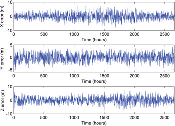
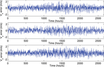
The newly updated state is then propagated forwards to the time of next observation and the time and measurement updates are repeated. An example of the WSB trajectory mentioned above is outlined, where the series of sail-to-spacecraft range observations are generated every 100 seconds and a position-only white-noise error of σnoise = 5 m is added to compensate for the stochastic error in every range measurement. After generating the observation data, then the EKF is employed to estimate the states of the spacecraft. Several simulations results are presented in Figures 11 and 12.
Position estimation error for the WSB trajectory with EKF algorithm.

Velocity estimation error for the WSB trajectory with EKF algorithm.

It can be seen from Figures 11 and 12 that the estimating process of the position and velocity components are all convergent. The maximum position estimation errors obtained by the EKF are 7.81 m, 4.92 m and 8.19 m respectively for the x, y and z components and the Root-Mean-Square (RMS) position errors are 2.40 m, 1.66 m and 2.43 m respectively. The maximum velocity estimation errors are 2.119 m/s, 2.077 m/s and 2.168 m/s, respectively for the v x , v y and v z components and the RMS velocity errors are 0.645 m/s, 0.661 m/s and 0.674 m/s respectively. The simulation results have demonstrated that the navigation constellation system by displaced solar sail can achieve a navigation accuracy of a few metres and have a good navigation performance in cislunar space.
6. CONCLUSION
This paper proposes a cislunar navigation constellation by displaced solar sails in which solar sails take the place of satellites to move around the artificial Lagrangian points. In the sail-CR3BP model, the regions of infinite artificially generated equilibria are demonstrated and used to construct the candidate constellation. Then, the candidate architecture of the navigation constellation works as the first-layer optimisation to decrease the average lightness number at the ALP. Next, the Hamiltonian structure-preserving controller and differential evolution algorithm work as the second-layer optimisation to generate a bounded quasi-periodic trajectory near the ALPs with minimum lightness number control. The navigation simulations for the cislunar WSB trajectory indicate the sail constellation system can provide a relatively high-performance navigation support for future Moon exploration.
The navigation constellation by displaced solar sails has two improvements: one is the radiation pressure of sail considered in a restricted three-body problem breaks the restriction on the number and plane of the classical Lagrangian points with large numbers of ALPs, which greatly enlarges the selectable range of sail constellations; the other is that the design based on the optimisation of lightness number validates the feasibility of the sail navigation constellation from two aspects of implementation in the mechanism and navigation performance. Due to the improvable navigation accuracy, the solar sail navigation system may have a great potential in the future.
However, there still remain some open problems. For instance, the navigation sail constellation is designed based on the minimum lightness number rather than the optimal navigation accuracy, thus there is much room for improvement of navigation performance via designing other constellation configurations, which will be considered in the following work.
ACKNOWLEDGEMENTS
This work was supported by the National Natural Science Foundations of China (11432001 and 11172020), the Fundamental Research Funds for the Central Universities. The authors are very grateful to Masoud Tofighzadeh for helpful discussions.