PRUSSIA AND AGRICULTURE

As we shall see, agricultural productivity across Prussia is best explained in the framework of a land-use model building on von Thünen.Footnote ¹⁰ This is in stark contrast to the conventional perspective that prevails in the literature on Prussia. Until the 1970s the institutional economics approach of the Younger Historical School represented by scholars like Georg Friedrich Knapp, Max Weber, and Werner Sombart dominated the historiography on Prussian agrarian reforms and agricultural development.Footnote ¹¹ These authors were convinced that the liberal agrarian reforms led to mass evictions of peasants and thus to the rise of an East Elbian rural proletariat. Moreover, they concluded that the rise of large, capitalist, and highly productive estates in the East was what allowed Prussia to feed its growing (industrial) population in the West.Footnote ¹² These scholars claimed, without much evidence, that agricultural productivity in the East was superior to that in the western part of Prussia. Overall, nineteenth-century Prussia was cast as a successful “continental” twin of England. It had been realizing a harsh but highly effective growth policy that allowed it to escape the Malthusian trap: liberal reforms in the East provided the labor force for German industrialization and established a domestic market for consumers industries.

This institutional approach has been challenged starting with historians who have shown that East Elbian agriculture was expanding long before the agrarian reforms.Footnote ¹³ There is little if any empirical evidence for a reform-induced agricultural takeoff. Moreover, recent studies on Westphalia have shown that agrarian reforms there also had little impact on growth or structural change in farming. Instead, it seems that the dynamics of market integration processes played a decisive role both before and after the reforms. After 1830 the variation across counties' participation in long distance trade with the rapidly expanding urban-industrial centers of the Ruhr, explains more than anything else the pronounced regional differences of agricultural growth within Westphalia. The extension of railways was also of decisive importance for a region's agricultural development. Regional agricultural growth as well as farming intensity was highly correlated to proximity to the demand center increasing the number of “cash products,” which could be profitably produced for the market. Moreover, the pronounced differences within Westphalia cannot be explained in terms of differences in the fertility of the soil. Rather, the decisive factor was that not all areas had equal access to the Ruhr.Footnote ¹⁴

Beyond access to markets, studies of nineteenth century Prussia have revealed a clear-cut West-East specialization.Footnote ¹⁵ Agriculture dominated in the eastern provinces and industry in the western Rhineland and Westphalia and in Saxony. Such specialization seems to support the long-held idea that the agrarian Prussian East had “fed the West.” Moreover, the higher East Elbian agricultural export share (relative to the Western parts of Prussia) is sometimes taken as evidence for eastern superiority. But one should be skeptical. First, even if the East had been exporting due to a comparative advantage in agriculture, this says nothing about absolute productivity. Second, the East was exporting only some particular products (grain) to some particular markets (especially Britain), but it sold little to the western parts of Prussia. Recent studies show that during the nineteenth century, domestic Prussian grain markets were highly fragmented.Footnote ¹⁶ Even after the political unification of Germany in 1871, a high degree of internal fragmentation remains with a strong internal East-West divide in domestic trade in agricultural as well as in other commodities.Footnote ¹⁷

Trade flows data confirm that long-distance imports played little role in feeding the densely populated Western provinces of the Prussian Empire.Footnote ¹⁸ Although the railway-based “transport revolution” after 1840 enabled a tremendous increase in domestic agricultural trade within Northwest Germany, it hardly increased food imports from other parts of the country. Despite the fact that connections between the Western and Eastern parts of Prussia improved, contemporary German sources suggest that few if any grain shipments went from the east to the west during the 1850s or 1860s, either by train or by ship. By the 1870s, when Northwest German grain production could not further satisfy local demand, grain imports from overseas rather from the Prussian east filled the gap.Footnote ¹⁹ From the beginning of Britain's industrialization until the “European grain invasion” East Elbia exported grain mainly to the British market, and to Central European cities such as Berlin.Footnote ²⁰

Baltic grain exports to Great Britain are well documented.Footnote ²¹ Liberals like Max Weber as well as Marxist historians concluded that early and strong international market integration gave Elbian large estates an advantage not only in market orientation but grain productivity as well. Wheat dominated Prussian grain exports to Great Britain. They rose from 25.405 tons in 1831–1835 to 163.673 tons per year in 1856–1860.Footnote ²² However, estimates of Prussian gross crop production around 1860 carried out as part of the land tax assessment by the famous mathematician Gauss strongly qualify wheat's role as an engine of agricultural growth. Gauss and the scholar Zachariae v. Lingenthal's estimates for the entire Prussian kingdom suggest that wheat only accounted for 4.6 percent of total grain production.Footnote ²³ Moreover, even if the entire wheat production of East Prussia and Pomerania had been exported around 1860, it would only amount to 14.5 percent of all grain production (or about 6 percent of the entire gross crop production) of these two provinces.

Hence, it looks as if the interaction between agricultural and wider economic development must have been predominantly shaped by local factors over most of the nineteenth century. We will argue that this fits into a picture where progress in agriculture is determined largely by the demand side—predominantly by local demand from cities. This is in line with our finding that agricultural productivity in the western parts of Prussia was clearly higher than in the East.

AGRICULTURAL PRODUCTIVITY IN NINETEENTH-CENTURY PRUSSIA: CONCEPTS, DATA SOURCE, DATA CRITIQUE, AND DESCRIPTIVE EVIDENCE

Our main indicator for agricultural productivity is the so-called Grundsteuerreinertrag (GRE), defined as the income from agrarian use of land less all costs of farmingFootnote ²⁴—in effect it is a version of the Ricardian rent.Footnote ²⁵ The GRE was stipulated by the tax administration as tax base for the land tax. To assess the tax, the administration wanted to determine the net revenue of land, according to quality, uses (arable, pasture, meadow, and horticulture), and location.

In contrast to nearly all other land tax assessments, the Prussian GRE is not based on schematic computations. Rather, the assessment of the net income per Prussian acre (GRE) was the result of an evaluation by experts assembled land tax assessment commissions (Veranlagungskommissionen).Footnote ²⁶ One such panel was established for each county. By law, their members were required to consider all factors which could affect a county's farming income. They had to travel through their counties to evaluate (farm) income per acre before tax for all kind of (farm) land and land classes.Footnote ²⁷ For this purpose, the commissions were obliged to pinpoint representative “exemplary parcels of land” (Mustergrundstücke) for every class of horticultural, arable, meadow, and pasture land, but also for woodland and lakes and ponds. For example, there were eight classes of arable land (Bonitätsklassen) representing different soil qualities reaching from “first-class wheat land” to the worst called “third-class rye land.” The assessed GRE of the “exemplary parcels of land” had to be consistent with local leases and prices of land. In the end, market prices were the most important check of the commissions' results. We have data at the level of all 342 Prussian counties on total GRE, and separately on GRE on arable, horticulture, pastures, and meadows.

The official guidelines for assessing the land tax required the netting out of operating costs (Bewirtschaftungskosten) from the value of output (Rohertrag). Output was defined as total gross crop production (including straw and all feed crops) from horticultural, arable, and grassland; thus it is gross output rather than marketed output.Footnote ²⁸ While the law prescribed a list of issues which had to be taken into account when assessing the costs of farming, the local tax commissions were not obliged to calculate costs separately.Footnote ²⁹ Beside unifying capital costs, all output and input positions had to be valued at long-term average local commodity prices (1837–1861) documented for every Prussian county by Meitzen and local agrarian wages.Footnote ³⁰ Detailed knowledge on local farming systems was thus necessary to assess the land tax. Much of this knowledge had been accumulated at different levels of the Prussian bureaucracy in the course of the agrarian reforms because it was essential to determine how much manorial peasants should compensate their former lords.Footnote ³¹

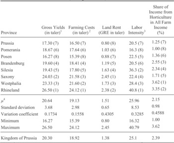
However, animal production and yields from livestock farming were not tabulated. The Prussian land tax regulation of 1861–1865 considered income from animal production only indirectly via its impact on arable farming and the profitability of grassland. This omission will tend to limit the effect from urban demand on agriculture (including animal production would thus only strengthen our findings). However, Engel, among others, suggested that the indirect effects from animal production, which are reflected in our GRE data must have been large.Footnote ³² The profitability and hence the spatial extension of high-yielding intensive farming systems as well as the success of grassland farming were driven mostly by an increase in feed demand of an expanding animal sector.Footnote ³³ Thus, the Prussian GRE does reflect effects from animal farming on arable and grassland farming to a large extent, but might still understate the effects of urban demand for animal products on agricultural productivity. Table 1 shows the data aggregated to the level of provinces. It also contains additional information from Engel on farming costs, which is only available at this higher level of aggregation.Footnote ³⁴

Table 1

GROSS YIELDS, FARMING COSTS, AND LAND RENT (per Prussian acre: 0.2553 ha) AND LABOR INTENSITY, 1865 (ranking in brackets)

Notes:

¹ = annual average monetary gross output per Prussian acre arable land; ² = annual average costs of farming a Prussian acre arable land; ³ = labor units per 100 hectare farm land; ⁴ = µ is an unweighted average (number of observations = 8).

Source:

Authors' own calculation based on Engel, “Preussen,” pp. 104–07; and Meitzen, Boden, vol. 4, pp. 116–17.

Overall, the Prussian GRE, which approximates net farm income per acre before taxes, corresponds to the concept of a land rent. A land rent is generally defined as the difference between the value of outputs and inputs. Hence, differences in GRE between counties principally reflect regional disparities in agricultural total factor productivity. According to several studies, long-run time series on real land rents based on data on land leases and net farm income per unit land roughly reflect secular developments of agricultural TFP.Footnote ³⁵ However, while the GRE will be highly correlated with TFP, the correspondence is imperfect by definition and more so if there are confounding price effects on the output or input side.Footnote ³⁶ To correct for output price effects, we deflate the nominal GRE with a (county-specific) crop price index in some of our tests (this deflation, however, makes little difference to our results).Footnote ³⁷ When it comes to input prices, we note that based on estimations of Engel on the level of Prussian provinces the variations of farming costs per acre showed only a quarter of the variation of gross yields.Footnote ³⁸ Thus, there is a potentially large role for differences in factor productivity. Differences in land rent (GRE) will therefore correctly reflect the ranking of counties' TFP, but will tend to overstate the variation in TFP. Notwithstanding these caveats, the Prussian GRE as a land rent reflects regional differences in agricultural TFP to a degree that at least it allows us to discriminate between low-, medium- and highly productive regions within the Prussian monarchy.Footnote ³⁹

A final caveat is in order. One might suspect that the GRE assessment was not carried out equally strict throughout the realm. In particular, the powerful Junkers in the eastern parts of Prussia might have been given preferential treatment. Lowering Junker's net revenues would obviously reduce their tax liabilities, but it would also penalize our measure of productivity in the East relative to other parts of Prussia. There are good reasons to doubt that assessment were biased. At 30 percent of all revenues, the land tax was a substantial source of income for the Prussian state. In fact, the land tax reform of 1861 met a central demand of the Liberals, whose power base was in the west, by abolishing most exemptions imbedded in earlier land taxes. These older systems had indeed heavily privileged the Eastern provinces and its nobility. That the tax reform was part of a political deal between the Liberals and the Prussian Crown makes a fair tax assessment all the more likely. The Crown's expensive military plans could be financed only with additional tax receipts, and these needed the consent of the Prussian parliament. In return, for higher taxes the government reorganized the land tax according to meet the demands of the Liberals. In fact, according to recent research 92 percent of the additional land tax burden fell on the Eastern provinces.Footnote ⁴⁰ Engel's in-depth investigation led him to conclude that the large regional differences in GRE cannot be explained by differences in assessors' valuations.Footnote ⁴¹ Furthermore, the Grundsteuerreinertag (GRE) was widely used by agricultural banks to determine the debt margin of a property or to estimate land prices. Even scholars who were very critical about the Junkers' privileges like Max Weber used the GRE data without restrictions. All contemporary experts agreed that the Prussian tax administration had made a thorough and honest determination of the net revenues.Footnote ⁴² Finally, a recent study of the Westphalian land market 1830–1860 concludes that no variable explains variations in observed land prices better than the Prussian GRE data; and in fact, it was used by contemporaries as an important benchmark to agree on land prices.Footnote ⁴³ In sum, the GRE data are a valuable source to explore regional differences in agricultural productivity across Prussia.

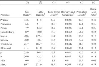
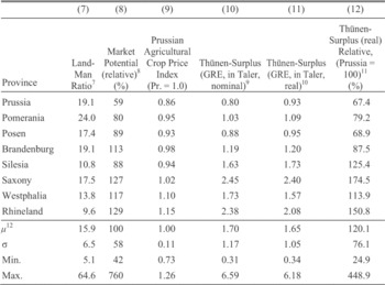
We refer to average GRE or land rent per unit farm land per county as the most comprehensive measurement of agricultural productivity available from our data, which can easily be computed out of Meitzen's data.Footnote ⁴⁴ Farmland comprises four categories: arable, horticultural, meadows, and pastures. Let us now consider the geographical patterns in the data. Tables 2A and 2B and Map 1 clearly suggest that there were huge differences in agricultural productivity as measured by the GRE (Table 2B, columns 10–12) and its possible determinants (Tables 2A and 2B, columns from 1 to 8). Some counties achieved only a quarter of the Prussian average real GRE whereas others exceeded it more than three times (column 12, lower panel). Even if we assume that variation in TFP is only about a fifth of the variation in GRE, these results suggests that agricultural TFP in the most productive counties was still between two and three times the level of TFP in the least productive ones.

Map 1 shows that agricultural productivity (real GRE per Prussian Morgen) follows a clear west-east gradient of decreasing performance only interrupted by central Germany and a minor region in Silesia.

Three compact regions have outstanding performance: (1) the northern Rhineland and parts of the bordering Westphalian Hellweg stretching as a broad strip located close to the southern Westphalian uplands around 100 km from Bochum to Lippstadt, (2) nearly the entire central German province of Saxony, and (3) a sizeable area in the western part of Silesia. A large regional block of average productivity includes Brandenburg, the rest of Silesia, and the western half of Pomerania. The most eastern provinces of the Prussian Kingdom Posen and the province of Prussia as well as the eastern half of Pomerania formed a large area with the lowest productivity—with very few exceptions around Danzig and Königsberg. However, even in the Rhineland and Westphalia smaller low productive regions could be located either in the unfertile uplands or distant from the Rhine-Ruhr industrial belt in Northern Westphalia. In the next section, we consider data on some of the potential factors behind this pattern.

POTENTIAL DETERMINANTS OF AGRICULTURAL PRODUCTIVITY

A first view on the data in Table 2 suggests several determinants of variations in agricultural productivity. Especially differences in soil quality as measured by the percentage share of top soils in total usable land (column 1) and population density (column 5) seem to be highly correlated to variation in productivity. Map 2 shows that the pattern of soil quality is roughly similar to the pattern of GRE per area. The best soils can be found in the Western territories, in Saxony and in Silesia.

Table 2A

AGRICULTURAL PERFORMANCE AND ITS IMPORTANT POTENTIAL DETERMINANTS IN PRUSSIAN PROVINCES, ABOUT 1865 (Prussian acre: 0.2553 ha)

Table 2B

AGRICULTURAL PERFORMANCE AND ITS IMPORTANT POTENTIAL DETERMINANTS IN PRUSSIAN PROVINCES, ABOUT 1865 (Prussian acre: 0.2553 ha)

Notes:

¹ = Share of high quality soils in the total area (in percent); ² = cattle per 1,000 acres of farmland; ³ = draught horses on farms per 1,000 acres of farmland; ⁴ = Kilometers of tracks and waterways per 100 Prussian square miles (1868); ⁵ = population per km² (1864); ⁶ = farm horses per unit labor; ⁷ = farmland per agricultural labor unit; ⁸ = for the formula, see the text; ⁹ = GRE is defined as net income out of farming per Prussian acre agricultural land (Grundsteuerreinertrag, see text); (10) = GRE(nominal) weighted by the Prussian agricultural crop price index (see the text); (11) = GRE(real)Province/GRE(real)Prussia; and (12) = μ is an unweighted average (number of observations = 327 counties).

Source:

Authors' own calculations based on Meitzen, Boden, vol. 4.

The GRE data seems also to vary systematically with access to food markets of urban-industrial agglomerations. GRE per area is highest in provinces with highest population density (column 5), which in turn depends on the number and size of cities. But the population, especially urban population, of neighboring regions should matter as well. So, we construct a simple measure of access to urban demand or “market potential” in the spirit of C.D. Harris.Footnote ⁴⁵ We define the geographic neighborhood to include not only Prussia but also all adjacent foreign territories (a total of about 50 European regions from Kurland in the North-East, Sweden and Denmark in the North over the Netherlands, Belgium and Alsace-Lorraine in the West, Bavaria in the South, and the Kingdom of Poland in the East). Then, we take the urban market potential of a county to be the distance-weighted sum of the urban populations from the entire sample:

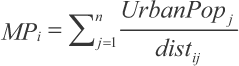
Table 2, column 8 and Map 3 presents the results given as market potential relative to the sample average.

The data show a clear west-east pattern with generally the highest access to urban demand in the Rhineland, Westphalia, and Saxony, but also fairly high levels of market potential in the neighborhoods of Berlin and Danzig. However, within these larger regions there is substantial variation. For example in the Rhineland, the two southern administrative districts of Trier and Koblenz lag far behind those of Düsseldorf or Cologne. Such variation should help us to identify the effect of market access on productivity controlling for other factors. In addition, our measure of market potential shows a spatial pattern of “rings” around major cities, most visible in the west but detectable as well in the East with Saxony and the greater area of Berlin at the center.

Map 1

NORMALIZED REAL LAND RENTS (GRE) PER PRUSSIAN MORGEN FARMLAND, 1865 (Prussian average = 1.0)

Source: Authors' own map.

MAP 2

SHARE OF HIGH-QUALITY SOILS IN TOTAL AREA, 1865 (in percent)

Source: Authors' own map.

MAP 3

NORMALIZED MARKET POTENTIAL, 1865 (Prussian average = 1.0, distance weighted sum of potential urban food demand)

Source: Authors' own map.

Most of the other factors that could affect productivity like population and cattle density, or transport infrastructure have systematically higher values in the Western parts of Prussia (including Saxony) than elsewhere and seem to be positively correlated to GRE (see Tables 1 and 2). The East was superior only with respect to farm horse density, especially East and West Prussia, which were famous horse breeding areas. Furthermore, all these variables show a large variance within relatively small areas. Looking at the descriptive statistics in Table 2A, this is true for soil quality (see also Map 2), market potential (Map 3), and transport infrastructure but as well to a lesser degree for cattle and farm horse density.

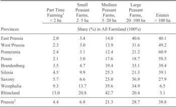
Finally, let us consider differences in farm structures. It is still an open question to what extent farm size affected productivity within nineteenth-century Prussia, not at least because the data are limited. Table 3 displays the size distribution of farms by province in 1882 (aggregated from data on 25 administrative districts). It shows that the relationship between farm structure and productivity in nineteenth- century Prussia was far from clear-cut. Whether small or large farm units could operate more efficiently seemed to depend on factors like soil quality and market access. It has been argued that nineteenth- century European industrialization provided conditions favorable to family farming, because smaller farms were best suited to meeting the demand of urban-industrial consumers.Footnote ⁴⁶ Indeed, the leading areas in the Prussian West and even more in Saxony had a wide range of different farm structures. On the whole, full-time family farms of very different sizes dominated but they also included estates between 75 ha and 150 ha as envisioned by von Thünen.Footnote ⁴⁷ However, there is no rule without exception. A smaller region of highly productive large estate farming seemed to exist around Breslau in Silesia. Moreover, parts of Pomerania around Stralsund enjoyed above average productivity despite poor soils, distant markets, and the dominance of large estates (with up to 80 percent of land in farms above 100 hectares). There is little evidence that the Rhineland or Westphalia were negatively affected by the lack of large estates or even lagged behind East Elbia.

Table 3

FARM STRUCTURE IN THE KINGDOM OF PRUSSIA, 1882 (operational units)

Notes:

¹ = The definition of farm classes follows the Prussian Statistic of 1882. Within these five categories the farm size classes are further differentiated; ² = Prussia in the borders of 1864. Reliable data on farm structure for the 1860s is not available. The Prussian farm statistics of 1882 refers on operational units and not on property in land or farms.

Source:

Author's own calculation based on Preussische Statistik, Ergebnisse, pp. 2–48.

The pattern of farm sizes is directly related to the various institutional legacies in different parts of Prussia. It is often been argued that establishing full private property in land was a revolutionary institutional change that caused an “agricultural takeoff.”Footnote ⁴⁸ Moreover, whether the “French” or “Prussian” or yet other reforms are best is fiercely debated. As noted in the introduction, we observe the legacies of very different agrarian reforms in Prussia. We consider the effect of the four variants of agrarian reform found in our 342 counties on agricultural productivity: (1) “Swedish Pomerania”: radical eviction of the peasants close to the English model (we code a dummy variable = 1 for the four counties of the administrative district of Stralsund); (2) East Elbian “Prussian reforms”: abolition of seigniorial rights with compensation mainly in land (we code a dummy = 1 for 239 counties of the Eastern and Central provinces of the Prussian Kingdom except Swedish Pomerania); (3) West Elbian “Prussian reforms”: abolition of seigniorial rights against redemption mainly in money (we code a dummy = 1 for 52 counties for the provinces Rhineland and Westphalia not annexed by France before 1815); (4) “French Revolution”: abolition without redemption of the nobility (we code a dummy variable = 1 for all 47 Rhenish counties annexed by France before 1815). Unsurprisingly, there is a clear relationship in the data between farm size in 1882 and the historical process of reform. Average farm sizes are highest in those regions where peasants were evicted without compensation (1) and lowest in regions, where the former rights of the nobility were abolished without redemption (4). Prussia acquired Swedish Pomerania only after 1815 forming the administrative district (Regierungsbezirk) Stralsund. In contrast to older Prussian territories, there was no royal protection (königlicher Bauernschutz) for peasant farms in Swedish Pomerania or Mecklenburg during the eighteenth century. Before 1815 Swedish Pomerania was ruled by its nobility and it was free of any royal demands for soldiers or revenues. Hence, after 1815 the commercially minded nobility evicted peasants on a large scale without compensation and carried out a rapid farm amalgamation after 1750. Thus, Stralsund was the only Prussian administrative district, whose property rights were shaped by an English-style eighteenth-century “landlords' revolution” as described by Robert C. Allen.Footnote ⁴⁹ In contrast, despite fierce resistance of the nobility, the Prussian agrarian reforms of the early nineteenth century allowed the majority of peasants to become full owner-occupiers of their farms. To be sure, they had to compensate their former lords either in land and cash in most parts east of the Elbe (2) or in cash only in the Prussian West (3). It is a myth that East of the Elbe the Prussian reforms caused the disappearance of the peasantry.Footnote ⁵⁰ Even if peasants lost land east of the Elbe, a large class of family farmers did emerge.Footnote ⁵¹ After 1815 Prussia also acquired territories on the left bank of the Rhine, where under French rule the seigniorial system had been abolished without compensation (4). There the Prussian government simply ratified the French reforms to keep the public peace.

Many factors might have contributed to the observed variation in agricultural productivity across Prussia. We must explore the channels by which they might have affected productivity and the relative significance of those different channels. In particular, we need to understand how access to markets outside of agriculture affects the geographical pattern of agricultural productivity. In the next section, we propose a simple model in the spirit of von Thünen that structures our further empirical work.Footnote ⁵²

A SIMPLE, TESTABLE VON THÜNEN FRAMEWORK

How does agricultural profitability (as measured by the GRE) vary with distance to urban demand, soil quality, and institutional legacies? To answer this question, we must clarify the relationship between land rents and distance to centers of demand. We consider a simple theoretical framework in the spirit of von Thünen by taking demand as given and exploring how supply decisions are shaped by distance from the location of demand.Footnote ⁵³ Next, we close the model with a simple demand function that depends on city size. The model is formulated as partial equilibrium for a specific crop that is defined by transport costs and a technology parameter. We will first characterize the partial equilibrium for one crop before we show (graphically) how in the model different types of crops will locate around the location of demand.

Building on the neoclassical land use model of M. J. Beckmann, let us assume that agricultural production is a function of two factors, land and labor, with constant returns to scale.Footnote ⁵⁴ All production is shipped to (and sold in) a central market, the city. Except from the location of cities, geography is a featureless plain. We abstract for the moment from additional input factors such as capital or local characteristics such as differences in soil quality, institutions, and the like. However, in our empirical investigation, we will have to control for these features. With this, we can formulate output per acre for a specific crop as a function of labor per acre (labor intensity) as

Rent per acre g(r, x) is then given by output valued at local prices net of factor costs, or

This formulation is very close to the GRE rent in our data, where land rents were calculated as the profit per acre valued at local prices, net of input costs (such as wages). The rent g(a, r, x) in equation 2 is sometimes called the “bid-rent” because it is the maximum price a farmer can bid for an acre of land at distance (r) from the city. This can also be seen as the minimum profitability a farmer needs to compete with other land uses (e.g., industrial plants) in the vicinity of a city.

Note that the formulation above assumes that there is only one type of crop. The parameter a in equation 2 reflects total factor productivity for a given crop and varies across crops, as explained below. Also, we value output at local prices, p(r). This is the per unit price of the good at the farm gate, hence net of transport costs at distance r from the market. Unlike Beckmann, we allow a more general form of transport costs.Footnote ⁵⁵ First, there is an ad valorem component (t₁) in the spirit of P. Samuelson), which increase in proportion to the value of goods shipped. Second, we allow for a per unit component (t₂) of transport costs that is independent from the value of transported goods.Footnote ⁵⁶ If we denote the price at the central market by (p) and the price at the farm gate at distance (r) from the central market by p(r), we have Note that the per unit component of transport costs does not vary in distance. However, the impact of that constant term on farm gate prices and therefore on land rents will increase with distance from the central market.

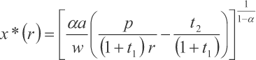
With a Cobb-Douglas production function, we can express output per acre as a function of labor intensity as It is straightforward to show that profit-maximization implies an increase in employment per acre the closer we move to the city (for details see the appendix). Profit-maximizing labor intensity x* can then be expressed as a function of parameters, prices, and distance to the central market as With this, the profit maximizing rent per acre g* is decreasing in distance to the city

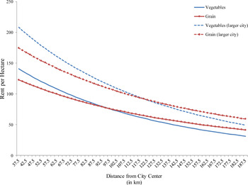
Equation 3 characterizes the partial equilibrium for one specific crop. Consider now the case of two crops, for example, vegetables and grain. Let us assume that these two goods differ in two dimensions: in their per unit transport costs (t₂) and in (a), their output per acre with one unit of labor input. Vegetables like lettuce or peas will be more costly to transport than grain for example because they can be more easily damaged and hence need to be handled with greater care. Figure 1 shows how the rent per acre changes for such two goods that differ only in their product per acre (a) and the per unit transport costs (t₂).

Consider first the two solid lines. The figure suggests that close to the city it will pay to grow products with high profits per acre but higher per unit transport costs (vegetables, eggs, or dairy products). Further out, it will be more profitable to produce goods with lower transport costs and lower profits per acre (grain, cattle). Furthermore profit-maximizing farmers will change factor inputs: the closer we move to the city center, the more expensive land becomes and farmers produce with more labor-intensive (land-saving) methods. Therefore, in two-dimensional space, the model generates the well-known von Thünen rings around the center of demand.

Figure 1

THE “BID-RENT” FUNCTION FOR VEGETABLES AND GRAIN AND DISTANCE FROM THE CENTRAL MARKET

Sources: Authors' own sources.

Furthermore, the size of the city (N) matters for farm profits. Given total supply (endowments, technology, and wages set outside the economy) and under some assumptions on the functional form of demand (which we provide in the Appendix to this article), the central market prices will increase linearly in city size as

At a given location, rents will increase with demand, given by city population N, and fall with transport costs, given by distance (r), or

The two dotted lines in Figure 1 show how a larger city will ceteris paribus shift the rent curves outwards. With this, our simple model has three testable implications.

First, rents will increase in the neighborhood of cities. More specifically, the model implies that rents will increase by more in the neighborhood of larger cities. We can approximate this relationship by a locations' access to urban demand or urban “market potential” as discussed in the section above.

Second, labor intensity will increase the closer we move to a city. According to the model, this is due to factor substitution in response to increasing land prices in the neighborhood of cities.

Third, an increase in average rent per acre will be partly due to an increase in farm gate prices (because of lower transport costs) and partly due to a change in crop mix towards higher yielding products that are more costly to transport. Therefore, the model predicts that variations in the average nominal rent per acre should be largely driven by variations in price levels and variations in productivity stemming from variations in the crop mix. In the next section, we will use our data to test these three implications.

WHAT EXPLAINS AGRICULTURAL PRODUCTIVITY ACROSS PRUSSIA?

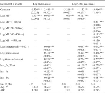
Testing the model, we analyze the connection between GRE and market demand in a series of regressions that all feature the 342 Prussian counties (Kreise) around 1865. All continuous variables are transformed to their natural logarithm so as to obtain elasticities. In a first step, we simply regress the log of GRE per area at the county level on a constant and on the log of accessible urban demand. Table 4, columns from 1 to 4, gives the result of a simple OLS regression (with Huber-White heteroskedasticity robust standard errors).

In column 1, the dependent variable is the nominal GRE; in column 3, we deflate the GRE using a county-level index of agricultural prices. Access to urban demand alone explains 44 percent of all the variation in nominal rents per acre in the sample and about one-third of the variation in real rents per acre that should better reflect the variation in productivity across Prussia. This suggest that our model captures a quite important aspect of agricultural development, but also that this is not the entire story. Next, in columns 2 and 4 we add several variables to control for differences in soil quality, institutional legacies (as captured by the dummies one to four, where we exclude two as an omitted category), as well as horses per area to proxy for capital, and transport infrastructure per area. All variables are significant at conventional levels and come with the expected sign. Adding these control variables reduces the coefficient on market access somewhat, but it stays large, positive, and highly significant. In the last column 5, we modify the model to allow for a differential effect of distance-weighted urban demand from nearby compared to distance-weighted demand from urban centers further away. To be specific, we distinguish between the effect of access to urban markets in a range up to 150 km, up to 300 km, up to 450km and above. We tried several other specifications with similar findings. The results show that access to more local urban demand exerts a much stronger effect on rent than access to centers further away.

Table 4

WHAT EXPLAINS AGRICULTURAL PRODUCTIVITY ACROSS PRUSSIA?

* = Statistical significance at the 10 percent level.

** = Statistical significance at the 5 percent level.

*** = Statistical significance at the 1 percent level.

Sources:

Author's own calculation. For data, see Meitzen, Boden, vol 4. Robust standard errors are in parentheses.

The simple regression in column 5 of Table 4 explains about two- thirds of the variation in our sample in terms of rent. It strongly suggests that access to urban demand is a crucial factor for agricultural rents. Moreover, the results concerning our institutional variables—especially the significant positive impact of our variable “Swedish Pomerania” on land rents—suggest that in some places at least labor-shedding and farm amalgamation led to higher rent and profitability in mid-nineteenth-century Prussia. In the middle of the nineteenth century, the Baltic regions produced grain for export to Britain. These exports were produced in a variant of the convertible husbandry system, that was quite extensive and labor-saving. Remarkably, this region had already been analyzed by Thünen himself. He concluded that Baltic large estates could not profitably implement the highly intensive (“Belgian farming model”) recommended by many agricultural experts for all of Germany.Footnote ⁵⁷

Could grain exports from other parts of Prussia, such as Pomerania or the provinces of East and West Prussia have spurred agricultural rent? To test for this more directly, we also ran regressions (not reported) where we controlled for the average (or minimum) distance to the five major grain export ports in the Baltic around the time, namely Memel, Pillau, Danzig, Swinemünde, and Rostock. If indeed grain exports had a positive effect on rent, we would expect to see that average (resp. minimum) distance to these major export ports should tend to reduce the GRE per area. Instead, we find the opposite. The log of distance to major ports comes with a significantly positive coefficient, whether we add this as an additional control to the variables in Table 4, columns 2 or 4, whether we simply regress rent on this distance variable alone, or whether we restrict the sample to counties east of the Elbe only. While our findings on the effect of access to urban demand and the other variables remain largely unchanged, we cannot find any evidence that grain exports via Baltic ports had a positive effect on agricultural rents.

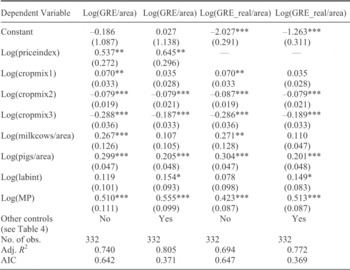
The next step involves exploring whether access to urban population matters for agricultural rent indeed through the channels suggested by our model, namely through variation in prices and crop mix. To see this, we rerun the regressions from Table 4 but add variables that should capture at least part of the effect of market access. To this end, we first create variables “cropmix1,” “cropmix2,” and “cropmix3” to capture variation in the type of agricultural output on which we have data. “Cropmix1” is defined as a county's GRE derived from horticulture (such as vegetable and fruit production) relative to the county's total GRE. In turn, “cropmix2” is defined as a county's GRE derived from meadows and “cropmix3” a county's GRE derived from pastures relative to the county's total GRE. Given that horticultural products tend to have higher transport costs per unit of weight but also higher value per unit, we expect that the share of the first will increase in the neighborhood of urban demand. In contrast, output derived from both meadows and pastures is most land intensive and hence its share should decrease in the neighborhood of urban demand, where land prices tend to be higher. Hence, we expect that these variables capture at least some part of the effect of access to urban demand on output per area, the first with a positive sign in the regression, the second and third with a negative sign. In addition, we include controls for the number of pigs and milk cows per agricultural area to capture a bit better the large indirect effects that animal production in the vicinity of cities should have on farming.Footnote ⁵⁸ In line with our theoretical framework we also add a control for labor intensity, measured as agricultural labor per agricultural area in a county. This should capture the effect in the model that profit maximizing farmers in the neighborhood of a city will try to adjust to the change in relative factor prices and substitute labor for land. Finally, whenever we use nominal values of GRE as dependent variable, we also add a control for the index of agricultural prices at the county level, which should capture the price-level effect of city size in the model. We expect prices to increase in the neighborhood of cities and hence enter with a positive sign.Footnote ⁵⁹

In Table 5, columns 1 to 4 we show to what extent we can explain the effect of access to urban markets on agricultural rent by these various channels, without and with adding the remaining controls for soil quality, capital, transport infrastructure and institutional legacy. Columns 1 and 2 show the effect using nominal GRE, hence adding a control for price effects, while columns three and four show the effect using deflated GRE.

Table 5

EXPLORING THE MECHANISM

* = Statistical significance at the 10 percent level.

** = Statistical significance at the 5 percent level.

*** = Statistical significance at the 1 percent level.

Source:

Author's own calculation. For data, see Meitzen, Boden, vol. 4. Robust standard errors are in parentheses.

As suggested by theory, crop mix, labor intensity and price effects rise in the neighborhood of large urban demand. Moreover, all these factors affect agricultural rent as measured by nominal or deflated GRE per area in the expected way. As suggested in the earlier literature on Britain and France, Prussian farmers adjusted to increases in demand by intensifying production and moving towards higher value crops.Footnote ⁶⁰ We can “explain” the effect of access to urban demand on agricultural rent by controlling directly for the various channels suggested by theory. The coefficient on market access declines—depending on the specification—by 40 percent with additional controls for institutional legacy, soil quality and others (compare coefficients in Table 4, columns 2 or 4 to those in Table 5, columns 2 and 4); or by up to 60 percent without these controls (compare coefficients in Table 4, columns 1 and 3 to those in Table 5, column 1 and 3). The fact that access to urban demand continues to affect agricultural rent after controlling for several channels probably reflects the limitations of our data. For example, we capture variation in the composition of agricultural production very imperfectly, based on a distinction between net output from the four categories horticulture, farming, pastures and meadows only. Obviously, there were differences within these four categories that we cannot deal with. Moreover, there might be additional channels, which are neglected in our theoretical framework, through which large cities affect their agricultural hinterland. Most notably, we do not take into account that there might have been spillover effects of technological and organizational change from urban-industrial agglomerations on agriculture.

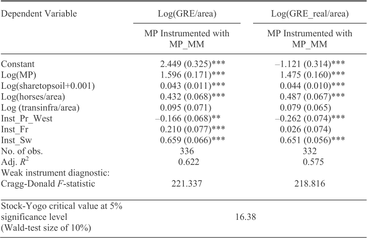
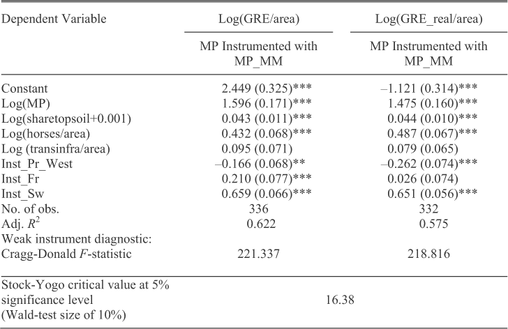
Before we can conclude that access to markets indeed mattered for agricultural rent, we need to address the issue that causation might have run the other way—not from urban demand to increases in agricultural rent, but rather from agricultural productivity to the formation and growth of cities and then to rent. Put differently, is it possible that urban demand (and its location) is actually endogenous to agricultural productivity? If so, our results in Tables 4 and 5 would be spurious. While a panel would be ideal, we are limited by data issues and use an instrumental variables approach. We need to address the issue that both the size of cities and their location might be endogenous to agricultural productivity. Hence, we need an instrument that is correlated to both the size and location of cities but independent of the exogenous components of agricultural productivity (e.g., soil type, climate, and institutional reforms). We propose to use the number of workers in industries that are heavily dependent on the existence of mineral resources, namely miners and workers in metal-processing industries, as an instrument for size and location of city population. To be specific, we construct a variable “access to miners and workers in metal processing” in the same way as we constructed the variable “access to urban population,” now calculated as the distance weighted sum of miners in a county and all other counties in the sample and use this as an instrument

Table 6, columns one and two show that this leaves our results largely unaffected. To show that the instrument is quite strong, we report the F-stat form of the Cragg-Donald statistic as suggested by Stock and Yogo as a test for weak instruments.Footnote ⁶¹ The values of that statistic are far above the critical value.

Table 6

IS ACCESS TO URBAN DEMAND ENDOGENOUS? IV-ESTIMATES

* = Statistical significance at the 10 percent level.

** = Statistical significance at the 5 percent level.

*** = Statistical significance at the 1 percent level.

Source:

Author's own calculation. For data, see Meitzen, Boden, vol 4. Robust standard errors are in parentheses.

With an IV-estimator, the coefficient on access to urban demand gets stronger, while notably our proxy for infrastructure weakens. This might suggest that the instrument captures some variation in the data that is related to access to urban demand but otherwise unaccounted for. A plausible candidate would be exactly the interaction between variations in infrastructure or other features affecting transport costs and urban demand that we capture in this setting only partially. Arguably, under the conditions of preindustrial agriculture science-based industrial inputs, technological and organizational spillover effects of the urban-industrial economy on agriculture did not yet exist. In Prussia around 1870 the prevailing biological-technical change was largely based on new crop rotations, seeds and breeds as well as all inputs that nearly completely came out of the agricultural sector itself.Footnote ⁶² However, important spillover effects of the urban economy on agriculture seemed to exist in agricultural trade that could benefit from a dense and often complex food trading network, which substantially reduced transaction costs.Footnote ⁶³ While we could try to improve on the measurement of access to markets, this would most likely leave our main result unaffected: access to urban markets is a key determinant of agricultural productivity and not by itself explained by productivity. Moreover, we assumed so far that real income per person is equal across counties and also that demand per person is homothetic. Both assumptions are not likely to hold. With either higher real wages in counties with higher employment in mining and metal industries and/or nonhomothetic demand for higher valued agricultural products such as vegetables or meat, the effect of demand on rents should get stronger.Footnote ⁶⁴ Crucially, all this (trading network effects, higher income in cities or nonhomothetic demand) makes our main finding even stronger: access to demand is a causal factor for agricultural development.